


1. Introduction
The use of fast waves in the lower hybrid range of frequencies, referred to as ‘helicons’ or ‘whistlers’, is currently being pursued as a means of heating and current drive in reactor-grade plasmas (Van Compernolle et al. Reference Van Compernolle2021). Helicon waves are a promising means for driving off-axis current in future tokamak devices (Prater et al. Prater et al., Reference Prater, Moeller, Pinsker, Porkolab, Meneghini and Vdovin2014). Reactor studies for advanced tokamak designs show that an important fraction of the total plasma current must be driven off axis (Jardin et al. Reference Jardin, Kessel, Bathke, Ehst, Mau, Najmabadi and Petrie1997). Lower hybrid current drive (LHCD) is typically considered for its high efficiency and power deposition at mid-radius. However, in reactor-grade plasmas slow lower hybrid waves at practical and accessible values of launched (normalized) parallel wavenumber, $n_\parallel$
, may have difficulty reaching the core of the plasma due to strong damping in the outermost part of the plasma. Helicons can have better accessibility to the plasma core and are less strongly damped than the slow wave used in typical LHCD schemes, so these waves can penetrate further into the plasma. With proper selection of the launched wave parameters, the power can be deposited at the desired mid-radius location (Pinsker Reference Pinsker2015).
$n_\parallel$
, may have difficulty reaching the core of the plasma due to strong damping in the outermost part of the plasma. Helicons can have better accessibility to the plasma core and are less strongly damped than the slow wave used in typical LHCD schemes, so these waves can penetrate further into the plasma. With proper selection of the launched wave parameters, the power can be deposited at the desired mid-radius location (Pinsker Reference Pinsker2015).
Launchers for these waves are mounted at the first wall of the device, and the plasma density immediately adjacent to the face of the launcher is significantly lower than the fast-wave cutoff density. Hence, the wave must tunnel through an evanescent layer until it reach densities above the fast-wave cutoff. Antenna coupling can change drastically as the plasma profile varies in front of the antenna face. In high-power systems it is imperative that changes in the antenna loading do not result in high levels of power reflected back to the radiofrequency (RF) sources. The traveling wave antenna (TWA) used in these experiments was designed to mitigate the effect of variations in plasma loading on the reflected power. The series of experiments detailed in this work were conducted on the LArge Plasma Device (LAPD) (Gekelman et al. Reference Gekelman2016) to verify a set of operational principles of the TWA design.
An overview of the experiment parameter space and a comparison with the DIII-D scrape-off layer (SOL) will be shown in § 2. A short introduction to the design of the antenna will be discussed in § 2.1. Thereafter, we will present the antenna design goals and corresponding measurements demonstrating that property of the operation. Section 3 discusses measurements of wave power relative to density cutoffs and upper limits. Section 4 shows the identification of both cold-plasma modes dependent on plasma density. Section 5 shows the directionality of the antenna; symmetry in the antenna structure allows feeding either end and launching waves with a preferred directionality relative to the static magnetic field. Section 6 discusses the relationship between the plasma density, the fast-wave cutoff density, and antenna loading. Section 7 shows a comparison of the measured wave fields with full-wave modeling. Lastly, § 8 concludes the paper with a summary of the results.
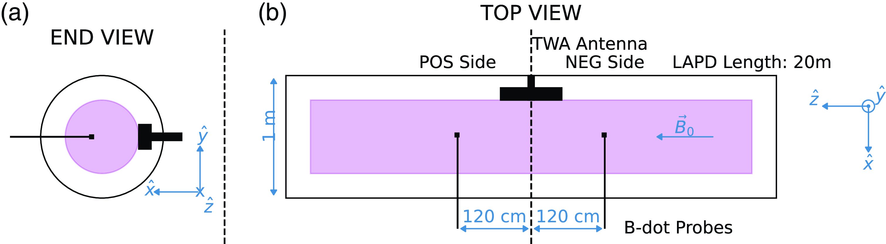
Figure 1. Diagram of LAPD (not to scale) illustrating relative probe positions and antenna side naming convention. (a) The XY cross-section showing representation of probe and antenna face; (b) the XZ cross-section showing antenna structure and probe separations. Here, POS/NEG side refers to the side with respect to $\hat {z}$
-coordinate or static magnetic field direction,
$\hat {z}$
-coordinate or static magnetic field direction, $\vec{B}_0$
.
$\vec{B}_0$
.
2. Experimental set-up
This paper details a set of experiments conducted on the LAPD, figure 1, at UCLA aimed to study the coupling and propagation of waves launched from a TWA of the comb-line type. At the time of these experiments the LAPD plasma was produced by a static fill of gas, helium in these experiments. A pulsed lanthanum hexaboride (LaB $_6$
) emissive cathode and molybdenum anode create the electron beam used to ionize the gas and create the plasma (Qian et al. Reference Qian2023). In this configuration densities of the order of
$_6$
) emissive cathode and molybdenum anode create the electron beam used to ionize the gas and create the plasma (Qian et al. Reference Qian2023). In this configuration densities of the order of $10^{18}$
m
$10^{18}$
m $^{-3}$
were routinely achievable with a plasma column diameter around 40 cm. More on density profiles will be discussed in subsequent sections. The static magnetic field,
$^{-3}$
were routinely achievable with a plasma column diameter around 40 cm. More on density profiles will be discussed in subsequent sections. The static magnetic field, $|\vec{B}_0|$
, was varied between 0.07 and 0.23 T; we take the 0.2 T case to be our ‘nominal’ operating condition for these experiments.
$|\vec{B}_0|$
, was varied between 0.07 and 0.23 T; we take the 0.2 T case to be our ‘nominal’ operating condition for these experiments.
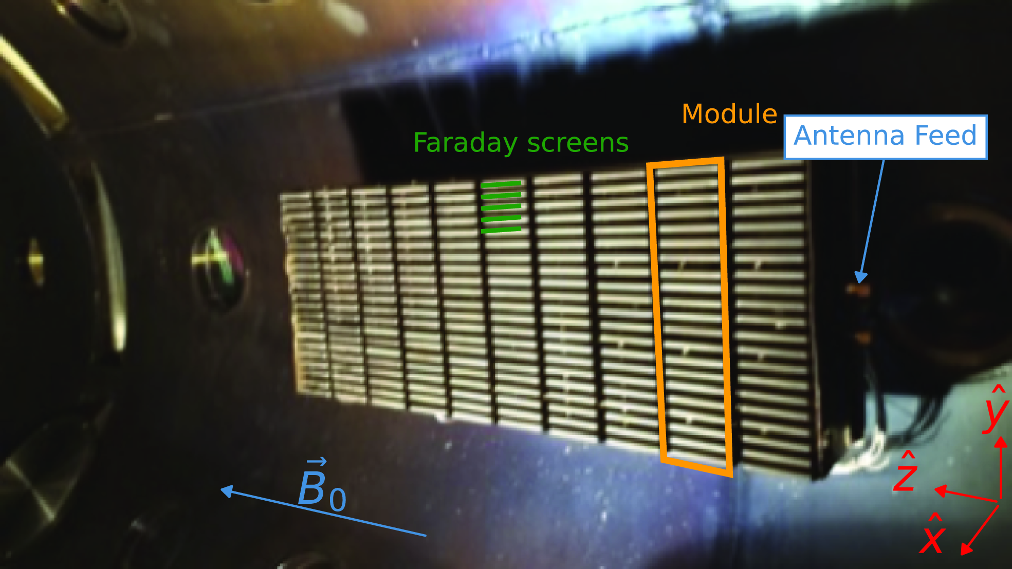
Figure 2. Photograph of TWA inside LAPD vessel. Antenna array has 10 individual modules, each with the current-carrying elements aligned in the $\hat {y}$
-direction. The array is nominally aligned with the static magnetic field (
$\hat {y}$
-direction. The array is nominally aligned with the static magnetic field ( $\hat {z})$
, but can rotate about the
$\hat {z})$
, but can rotate about the $\hat {x}$
-axis to skew the alignment of both the current-carrying elements and array with respect to the static magnetic field.
$\hat {x}$
-axis to skew the alignment of both the current-carrying elements and array with respect to the static magnetic field.
The antenna used (shown in figure 2) is constructed from a subset of the 12 low-power modules used on helicon experiments on DIII-D in 2016; the design of the elements and array are detailed in the literature (Pinsker et al. Reference Pinsker2018). The passband of the antenna is from 450 to 500 MHz, and the band center at 476 MHz is the nominal operating frequency for the antenna in these experiments. The modules are arranged in a linear array along the long axis of LAPD, parallel to the static magnetic field. The antenna structure consists of 10 modules, each of which is 5 cm wide, making the entire antenna structure roughly 50 cm along the axial direction. The structure is mounted so that it can be moved in the radial direction ( $\hat {x}$
in figure 1) as well as rotated relative to the static magnetic field (about the
$\hat {x}$
in figure 1) as well as rotated relative to the static magnetic field (about the $\hat {x}$
-axis). Table 1 summarizes the plasma and antenna parameters for LAPD in comparison with the typical DIII-D SOL. It should be noted that the large difference in magnetic field puts these wave in comparatively different regimes. In the LAPD case there is no combination of plasma and antenna parameters in which the waves can propagate up to the lower hybrid resonance density. A mode conversion or confluence point exists for all achievable configurations of frequency,
$\hat {x}$
-axis). Table 1 summarizes the plasma and antenna parameters for LAPD in comparison with the typical DIII-D SOL. It should be noted that the large difference in magnetic field puts these wave in comparatively different regimes. In the LAPD case there is no combination of plasma and antenna parameters in which the waves can propagate up to the lower hybrid resonance density. A mode conversion or confluence point exists for all achievable configurations of frequency, $n_\parallel$
(=
$n_\parallel$
(= $k_\parallel /k_0$
,
$k_\parallel /k_0$
, $k_0=\omega /c$
,
$k_0=\omega /c$
, $k$
is the wavenumber,
$k$
is the wavenumber, $\omega$
is the angular frequency,
$\omega$
is the angular frequency, $c$
is the speed of light), static magnetic field, and density (a discussion of the mode conversion point and wave accessibility can be found in Appendix B of Pinsker (Reference Pinsker2015)). Hence, the mode conversion point acts as an upper density limit for wave propagation in LAPD, i.e. determines wave accessibility. (In DIII-D, by contrast, there is no upper limit in density for accessibility of fast waves due to the
$c$
is the speed of light), static magnetic field, and density (a discussion of the mode conversion point and wave accessibility can be found in Appendix B of Pinsker (Reference Pinsker2015)). Hence, the mode conversion point acts as an upper density limit for wave propagation in LAPD, i.e. determines wave accessibility. (In DIII-D, by contrast, there is no upper limit in density for accessibility of fast waves due to the $\sim$
tenfold higher static magnetic field.) Although there may be a difference in wave regime, figure 3 shows a region in density space where both branches simultaneously propagate in the LAPD and DIII-D cases making this comparison of the operation of the TWA relevant. The achievable parameter space in LAPD is most representative of the low-density case in DIII-D which is indicative of the coupling region of the antenna.
$\sim$
tenfold higher static magnetic field.) Although there may be a difference in wave regime, figure 3 shows a region in density space where both branches simultaneously propagate in the LAPD and DIII-D cases making this comparison of the operation of the TWA relevant. The achievable parameter space in LAPD is most representative of the low-density case in DIII-D which is indicative of the coupling region of the antenna.
Table 1. Comparison of plasma and antenna parameters for LAPD TWA and DIII-D high-power helicon system.
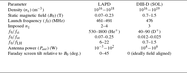
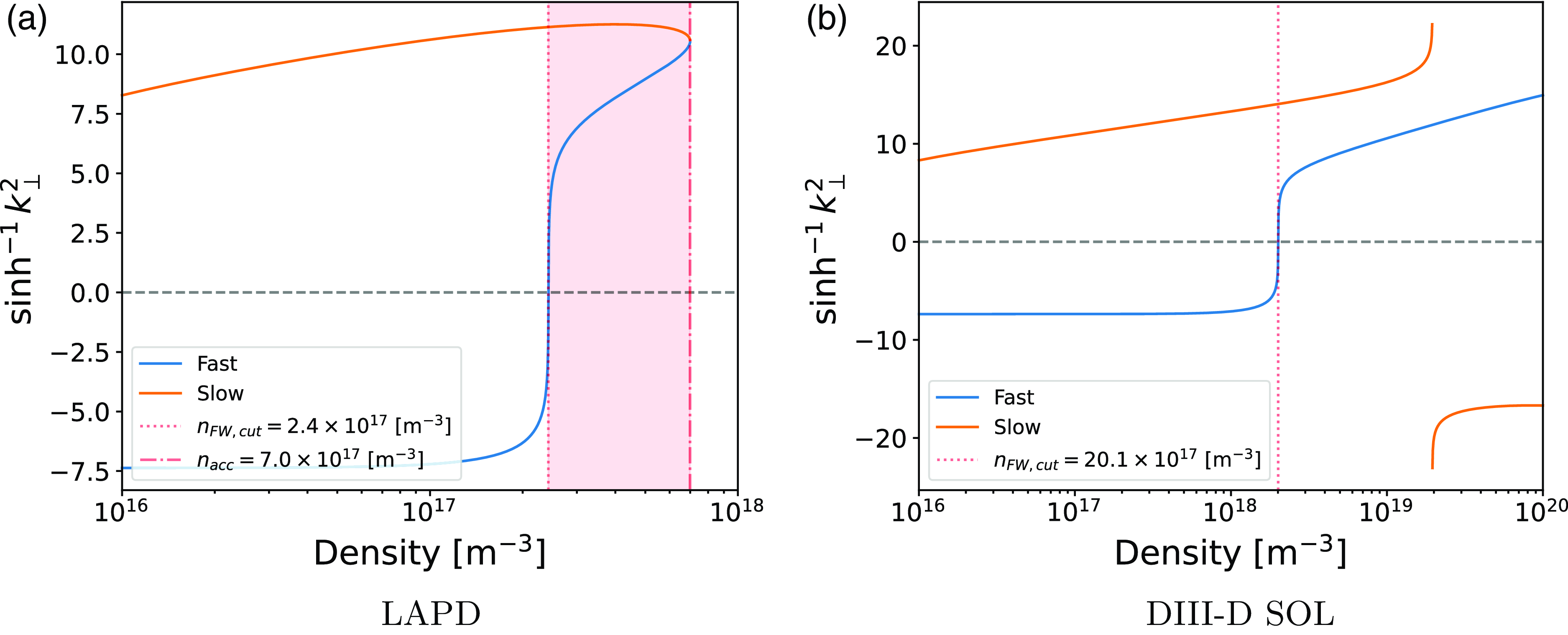
Figure 3. Comparison of wave regimes in (a) ‘nominal’ case in LAPD and (b) DIII-D SOL. Note LAPD has a significantly lower static magnetic field than DIII-D.
Figure 3 shows plots of the dispersion solutions against density for both the LAPD and DIII-D SOL cases. The quantity plotted is proportional to the perpendicular wavenumber squared. Negative values of this quantity correspond to non-propagating solutions. We can see in figure 3(a) there is no density at which the fast wave can propagate where the slow wave is evanescent. In contrast, figure 3(b) shows there is a high-density regime where only the fast wave can propagate in the DIII-D-relevant parameter space. This is an important difference as measurements of wave power and antenna loading in LAPD can always have contributions from both branches except at low density. As such, we must be certain to distinguish between the modes present in the plasma. The static magnetic field and $n_\parallel$
dependence of the dispersion solutions against density can be seen in figure 4. Panel (a) shows that as the field decreases both the fast-wave cutoff density and the confluence density decrease as well. Similarly, both the fast-wave cutoff density and confluence density decrease with a reduced
$n_\parallel$
dependence of the dispersion solutions against density can be seen in figure 4. Panel (a) shows that as the field decreases both the fast-wave cutoff density and the confluence density decrease as well. Similarly, both the fast-wave cutoff density and confluence density decrease with a reduced $n_\parallel$
(see panel b). For the parameters scans in the experiment this corresponds to fast-wave propagation at later discharge times for lower magnetic field configurations and lower imposed
$n_\parallel$
(see panel b). For the parameters scans in the experiment this corresponds to fast-wave propagation at later discharge times for lower magnetic field configurations and lower imposed $n_\parallel$
.
$n_\parallel$
.
Wave fields were observed with a set of magnetic induction ( $\dot {B}$
) probes. These probes were mounted on ball valves that allowed them to be moved within the LAPD volume by automated probe drives (Leneman & Gekelman Reference Leneman and Gekelman2001). Two probes were placed on either side of the antenna, separated from the antenna center by 1.2 m (as shown in figure 1). To map out the wave power profiles and spatial structure, a series of plasma shots were taken in data planes within the plasma volume. The probe was moved to a position within the data plane, 20 plasma shots recorded at the given position and then the probe was moved to the next data plane position. The sampling frequency limit on our primary data acquisition system was 100 MHz. The RF signals in these experiments were in the range of 0.5 GHz, and a set of mixing circuits were needed to digitize the RF signals. Additionally, the experiment was conducted over a long time window within the discharge. Had many RF signals been measured at a high digitization rate over a long time, unwieldy (and unnecessarily) large data sets would have resulted. The RF signals were mixed down to an intermediate frequency of 1 MHz, allowing for a digitization rate of 12.5 MHz to be used to help reduce the size of the data sets. Density measurements were made using a swept Langmuir probe. Spatially resolved density measurements were made in a similar fashion as the wave measurements, by moving the probe over many plasma shots. Additionally, a microwave interferometer was used to measure absolutely calibrated line-averaged density.
$\dot {B}$
) probes. These probes were mounted on ball valves that allowed them to be moved within the LAPD volume by automated probe drives (Leneman & Gekelman Reference Leneman and Gekelman2001). Two probes were placed on either side of the antenna, separated from the antenna center by 1.2 m (as shown in figure 1). To map out the wave power profiles and spatial structure, a series of plasma shots were taken in data planes within the plasma volume. The probe was moved to a position within the data plane, 20 plasma shots recorded at the given position and then the probe was moved to the next data plane position. The sampling frequency limit on our primary data acquisition system was 100 MHz. The RF signals in these experiments were in the range of 0.5 GHz, and a set of mixing circuits were needed to digitize the RF signals. Additionally, the experiment was conducted over a long time window within the discharge. Had many RF signals been measured at a high digitization rate over a long time, unwieldy (and unnecessarily) large data sets would have resulted. The RF signals were mixed down to an intermediate frequency of 1 MHz, allowing for a digitization rate of 12.5 MHz to be used to help reduce the size of the data sets. Density measurements were made using a swept Langmuir probe. Spatially resolved density measurements were made in a similar fashion as the wave measurements, by moving the probe over many plasma shots. Additionally, a microwave interferometer was used to measure absolutely calibrated line-averaged density.
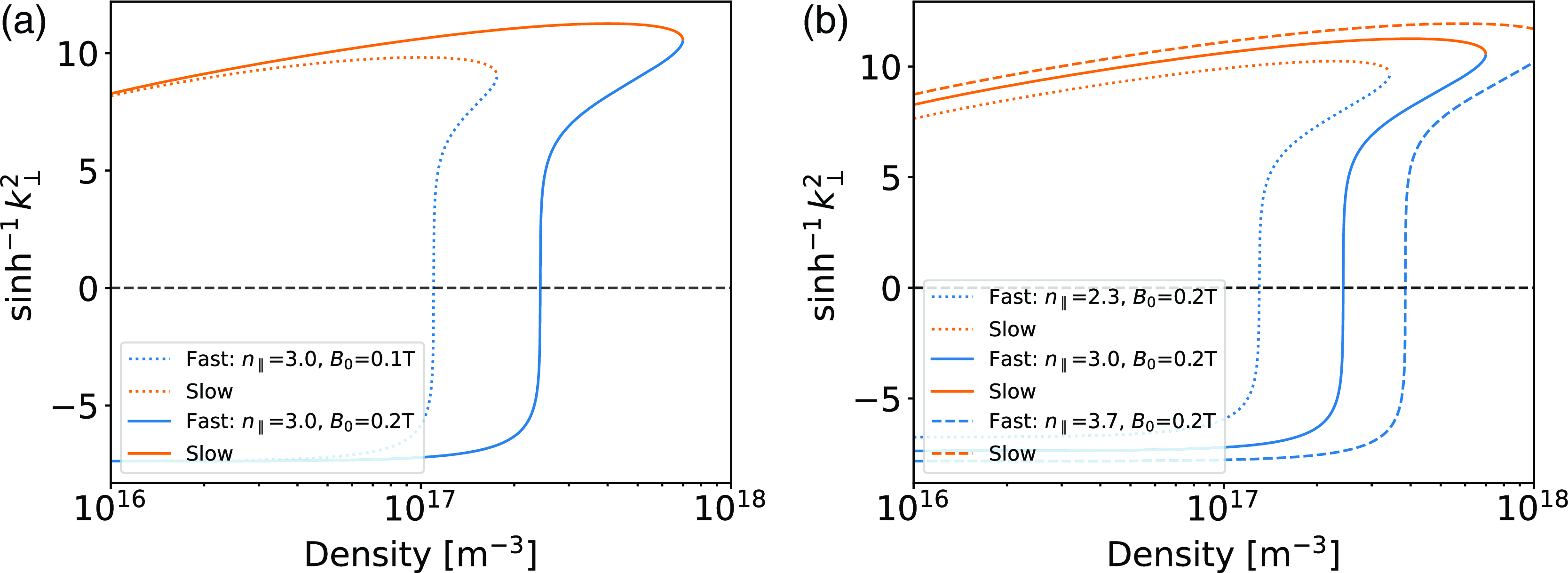
Figure 4. Comparison of LAPD relevant dispersion solutions vs density for: (a) two static magnetic field cases $B_0$
= 0.1, 0.2 T at
$B_0$
= 0.1, 0.2 T at $n_\parallel$
= 3.0; and (b)
$n_\parallel$
= 3.0; and (b) $n_\parallel$
= 2.3, 3.0, 3.7 at
$n_\parallel$
= 2.3, 3.0, 3.7 at $B_0=0.2$
T.
$B_0=0.2$
T.
2.1. TWA operation
The TWA used in these experiments is constructed from a subset of the modules used in the low-power helicon experiments at DIII-D . The design of the antenna is detailed in Pinsker et al. (Reference Pinsker2018). A summary of the operational principles follows. The set of modules are aligned along the direction of the static (axial) magnetic field. Each individual module has its current-carrying element aligned perpendicular to the static magnetic field. The coordinate system shown in figure 1 corresponds to the array being aligned in the $\hat {z}$
direction (
$\hat {z}$
direction ( $\boldsymbol{B_0}=B_0\hat {z}$
) and the current elements in the
$\boldsymbol{B_0}=B_0\hat {z}$
) and the current elements in the $\hat {y}$
direction (
$\hat {y}$
direction ( $\boldsymbol{J}=J_{\mathrm{mod}}\hat {y}$
). Power is fed into the antenna structure at one end, a fraction of the power is radiated to the plasma and residual power is mutually coupled to the subsequent module. The inner modules are each fed through the mutual inductive coupling to the previous ‘upstream’ module. The last module has a feed through so that any uncoupled power can be dissipated in an external 50 Ohm dummy load. The antenna launches waves directionally, with the sign of the axial component of the launched wavevector determined by the selection of which end of the antenna is fed. The direction of the wave launch follows the direction of the power flow along the antenna array.
$\boldsymbol{J}=J_{\mathrm{mod}}\hat {y}$
). Power is fed into the antenna structure at one end, a fraction of the power is radiated to the plasma and residual power is mutually coupled to the subsequent module. The inner modules are each fed through the mutual inductive coupling to the previous ‘upstream’ module. The last module has a feed through so that any uncoupled power can be dissipated in an external 50 Ohm dummy load. The antenna launches waves directionally, with the sign of the axial component of the launched wavevector determined by the selection of which end of the antenna is fed. The direction of the wave launch follows the direction of the power flow along the antenna array.
The feed for one end can be seen in figure 2, but is identical on the other end of the antenna array. The antenna array is symmetric, so by exchanging the feed end and dummy load, power can be coupled into the opposite end of the antenna. This exchange results in a change of the sign of the principal imposed parallel wavenumber and change in the directionality. The design is such that the input impedance of the antenna structure is largely determined by the mutual coupling between antenna modules rather than the plasma loading of any one individual module. This results in small changes in the reflected power for variations in the plasma at the antenna face. That is not to say that antenna loading is unaffected by changes in the plasma. Changes in the absolute density and density profile can affect the antenna loading, as will be shown in § 6. The loading is characterized by the rate of decay in the power measured along the array. A series of RF pick-up loops are integrated into each module to measure the power at any given module. The phase jump between modules shifts as the frequency is varied within the pass-band of the antenna. Figure 5 shows a model of the antenna frequency $f$
response where the phase jump ranges from 0 to
$f$
response where the phase jump ranges from 0 to $\pi$
as the applied frequency is varied from the lower to upper edges of the passband (Van Compernolle et al. Reference Van Compernolle2021). The phase jump, module size and separation determine the imposed parallel wavenumber spectrum the antenna excites. Therefore, a change in the drive frequency of the antenna results in a change in the principal imposed parallel wavenumber.
$\pi$
as the applied frequency is varied from the lower to upper edges of the passband (Van Compernolle et al. Reference Van Compernolle2021). The phase jump, module size and separation determine the imposed parallel wavenumber spectrum the antenna excites. Therefore, a change in the drive frequency of the antenna results in a change in the principal imposed parallel wavenumber.
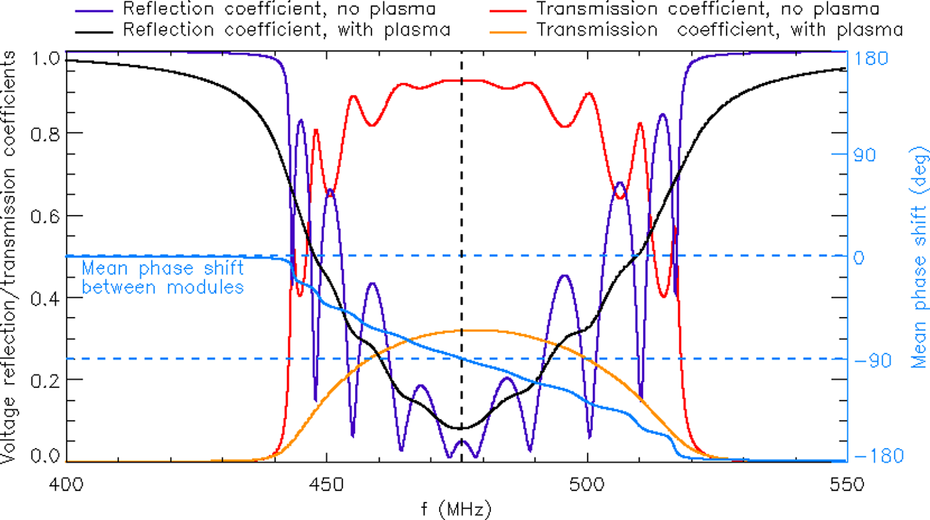
Figure 5. Model of antenna transmission, reflection coefficients and phase shift between modules over the passband of the antenna array.
3. Wave accessibility
Here, we will explore the wave measurements as related to wave accessibility. As seen in figure 3(a) the range of densities in which the fast wave can propagate in LAPD is small (denoted by the red highlighted region), less than an order of magnitude separates the minimum and maximum densities at which the fast wave can propagate for the nominal case. The low-density limit is set by the fast-wave cutoff density. The upper density limit is set by the confluence or mode conversion point of the two branches. This density is the point where the two branches become indistinguishable. A fast wave propagating in towards this density mode converts to an outward-propagating slow wave due to conservation of the direction of $\boldsymbol{k}$
and radially backward nature of the slow branch. Because both modes may simultaneously propagate in the LAPD, distinguishing between the two modes is imperative to assess the effectiveness of the antenna as a fast-wave launcher. We will explore a series of methods for experimentally distinguishing the two modes throughout the remainder of the paper.
$\boldsymbol{k}$
and radially backward nature of the slow branch. Because both modes may simultaneously propagate in the LAPD, distinguishing between the two modes is imperative to assess the effectiveness of the antenna as a fast-wave launcher. We will explore a series of methods for experimentally distinguishing the two modes throughout the remainder of the paper.
3.1. Density profiles
The accessible range of densities sets a region in which we expect to measure fast waves launched from the antenna. Having conducted these experiments throughout the entirety of the LAPD discharge, we sample density during the ‘afterglow’ portion of the discharge, i.e. after the discharge power is turned off and the plasma density decays in time. Figure 6(a) shows the time history of an LAPD discharge. The DC power to the discharge is switched off at t = 10 ms, so that the subsequent portion of the discharge is the ‘afterglow’, during which the density drops monotonically. The specific case shown is with the nominal $B_0$
= 0.2 T static magnetic field. The fast-wave cutoff density and the confluence density are shown for
$B_0$
= 0.2 T static magnetic field. The fast-wave cutoff density and the confluence density are shown for $f_0$
= 476 MHz,
$f_0$
= 476 MHz, $n_\parallel$
= 3.0. We can see that there is a limited time during the discharge where the line-averaged density measurement suggests that the plasma could support fast-wave propagation. Selecting a time during this window and using the spatially resolved density measurement, an example of which is shown in figure 6(b), we can characterize the spatial extent of the region that supports fast-wave propagation. Figure 6(b) also shows that the density across the machine is mostly flat, with the density rising from plasma edges but essentially flat across the central region
$n_\parallel$
= 3.0. We can see that there is a limited time during the discharge where the line-averaged density measurement suggests that the plasma could support fast-wave propagation. Selecting a time during this window and using the spatially resolved density measurement, an example of which is shown in figure 6(b), we can characterize the spatial extent of the region that supports fast-wave propagation. Figure 6(b) also shows that the density across the machine is mostly flat, with the density rising from plasma edges but essentially flat across the central region $-10 \leqslant x \leqslant 20$
cm. These density profiles allow us to construct a picture of where we might expect fast-wave propagation in our plasma across the field configurations, densities and launch frequency. Figure 7 shows the accessible region of densities as the area enclosed in the red contours. The solid red lines show the region in which the density was calculated using a swept Langmuir probe for density and temperature and calibrated against the microwave interferometer. After 10 ms we no longer had reliable temperature data from the probes, so a flattened out temperature profile was assumed to calculate the density from the ion saturation current and microwave interferometer, this region is denoted by the dotted red line contours. The two rows of figure 7 are for two static magnetic field cases (
$-10 \leqslant x \leqslant 20$
cm. These density profiles allow us to construct a picture of where we might expect fast-wave propagation in our plasma across the field configurations, densities and launch frequency. Figure 7 shows the accessible region of densities as the area enclosed in the red contours. The solid red lines show the region in which the density was calculated using a swept Langmuir probe for density and temperature and calibrated against the microwave interferometer. After 10 ms we no longer had reliable temperature data from the probes, so a flattened out temperature profile was assumed to calculate the density from the ion saturation current and microwave interferometer, this region is denoted by the dotted red line contours. The two rows of figure 7 are for two static magnetic field cases ( $B_0=0.1$
T and
$B_0=0.1$
T and $B_0=0.2$
T). In the higher-field case we note that there is a more extended region, both in discharge time and spatially, in which fast waves can propagate (as indicated in the dispersion relation shown in figure 4
a). As we increase the launch frequency (and thereby the magnitude of the imposed
$B_0=0.2$
T). In the higher-field case we note that there is a more extended region, both in discharge time and spatially, in which fast waves can propagate (as indicated in the dispersion relation shown in figure 4
a). As we increase the launch frequency (and thereby the magnitude of the imposed $n_\parallel$
) the accessible region of densities shifts to higher densities. Therefore, we expect fast-wave propagation later in the discharge (that is, at lower plasma density) at lower launch frequencies. The region outside the contours at late discharge times does not support fast-wave propagation because the density is below the fast-wave cutoff density everywhere in the plasma at that time. The slow branch can propagate at those low densities, so wave power measured at these times is likely to be due to direct excitation of the slow branch.
$n_\parallel$
) the accessible region of densities shifts to higher densities. Therefore, we expect fast-wave propagation later in the discharge (that is, at lower plasma density) at lower launch frequencies. The region outside the contours at late discharge times does not support fast-wave propagation because the density is below the fast-wave cutoff density everywhere in the plasma at that time. The slow branch can propagate at those low densities, so wave power measured at these times is likely to be due to direct excitation of the slow branch.
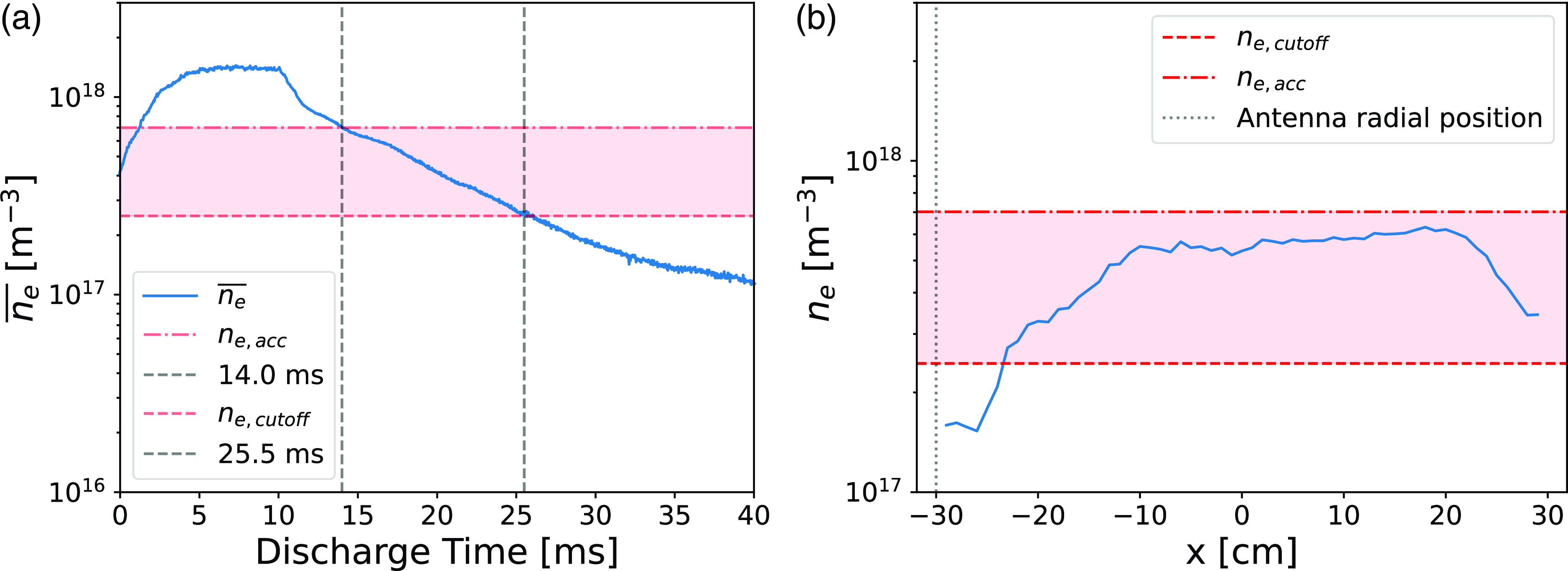
Figure 6. Density measurements in LAPD with $B_0=0.2$
T; (a) is the line-averaged density measured by an interferometer, (b) is a density profile across the radial axis of the machine at a selected time during the discharge (
$B_0=0.2$
T; (a) is the line-averaged density measured by an interferometer, (b) is a density profile across the radial axis of the machine at a selected time during the discharge ( $t=17$
ms) as measured by a Langmuir probe. Accessible region of densities shown for
$t=17$
ms) as measured by a Langmuir probe. Accessible region of densities shown for $f_0=476$
MHz and
$f_0=476$
MHz and $n_\parallel =3.0$
.
$n_\parallel =3.0$
.
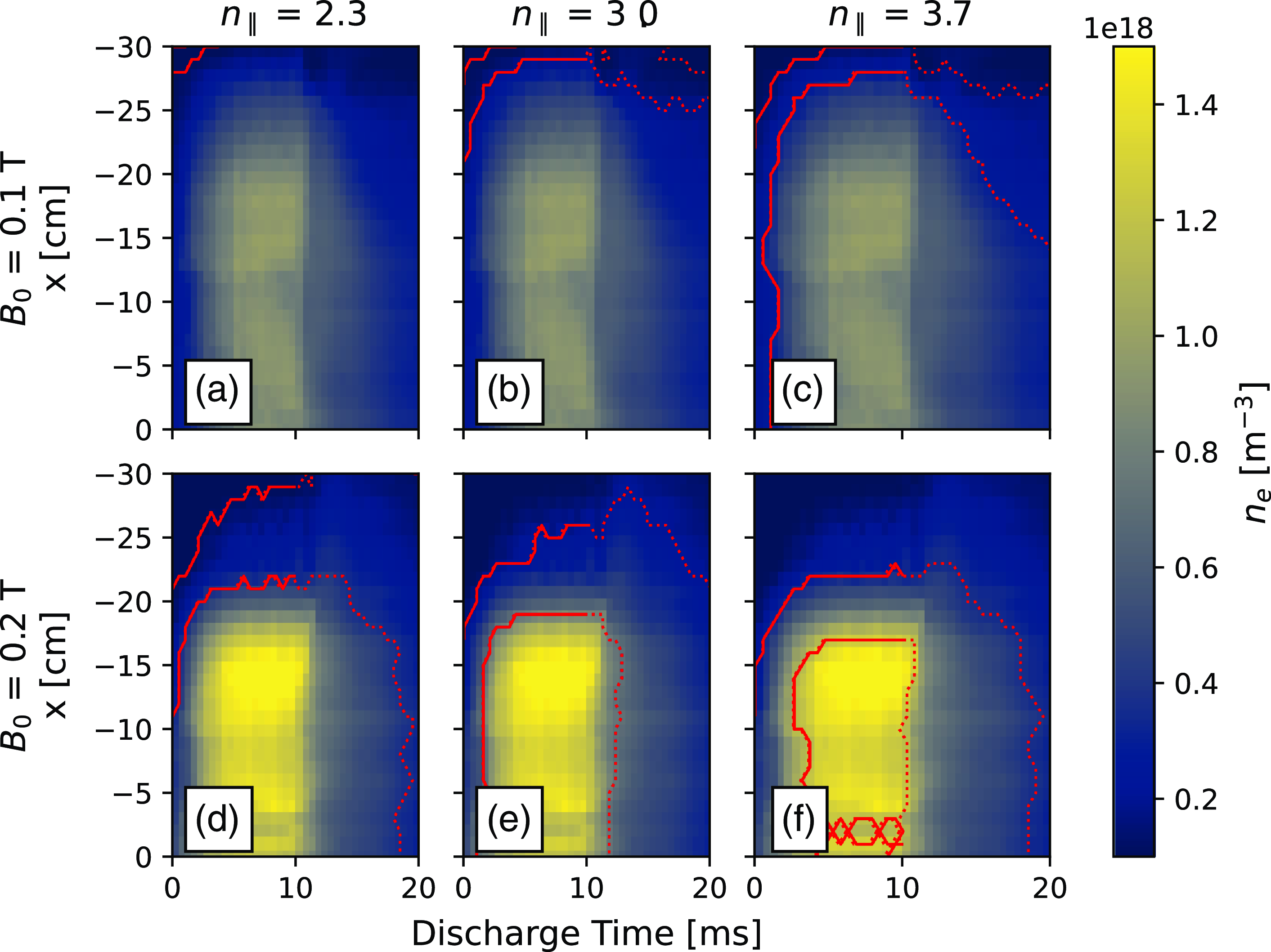
Figure 7. Measurements of density shown at two magnetic field configurations: $B_0$
= 0.1 T (a–c);
$B_0$
= 0.1 T (a–c); $B_0$
= 0.2 T (d–f). The color intensity of the image corresponds to the absolute density measurement from a Langmuir probe. Solid lines denote time where temperature profiles were included in density calculation from swept probes (0–10 ms). Overplotted is a contour of the accessible region of densities, i.e. densities between the fast-wave cutoff and confluence densities for a given combination of
$B_0$
= 0.2 T (d–f). The color intensity of the image corresponds to the absolute density measurement from a Langmuir probe. Solid lines denote time where temperature profiles were included in density calculation from swept probes (0–10 ms). Overplotted is a contour of the accessible region of densities, i.e. densities between the fast-wave cutoff and confluence densities for a given combination of $B_0$
and
$B_0$
and $n_\parallel$
.
$n_\parallel$
.
3.2. Wave amplitude measurements
Next, we can overlay the accessible region of densities onto plots of the measured wave magnetic fields. We compare the regions in which we measure wave power with the expected domain of fast-wave propagation. Within the overplotted contour both branches may propagate, so power measured therein may result from either the fast or slow branch excited by the antenna. Figure 8 shows measurements of the wave amplitudes for combinations of magnetic field and $n_\parallel$
. During early discharge times (
$n_\parallel$
. During early discharge times ( $t_{\mathrm{dis}}\leqslant 10$
ms), when the discharge is powered, we see significant wave power on the plasma edge. During this time in the discharge the edge density can fluctuate drastically due to drift waves. The simple picture of an time-average density profile does not entirely describe the wave propagation region during those times. Panels (d) and (e) in figure 8 show regions within the contours with significant measured wave power. It is clear from all the panels of figure 8 that there is significant wave power at late times in the discharge after the density has dropped below the fast-wave cutoff density across the plasma column. This suggests that, at these later times (lower densities), the antenna couples power directly to the slow mode. We will later, in § 6, show that at these late times the magnitude of the antenna loading is smaller when only slow wave coupling is present. While measurements of wave power at densities well below the fast-wave cutoff density suggests coupling to the slow mode, we can use characteristics of the two modes to further investigate the wave mode present.
$t_{\mathrm{dis}}\leqslant 10$
ms), when the discharge is powered, we see significant wave power on the plasma edge. During this time in the discharge the edge density can fluctuate drastically due to drift waves. The simple picture of an time-average density profile does not entirely describe the wave propagation region during those times. Panels (d) and (e) in figure 8 show regions within the contours with significant measured wave power. It is clear from all the panels of figure 8 that there is significant wave power at late times in the discharge after the density has dropped below the fast-wave cutoff density across the plasma column. This suggests that, at these later times (lower densities), the antenna couples power directly to the slow mode. We will later, in § 6, show that at these late times the magnitude of the antenna loading is smaller when only slow wave coupling is present. While measurements of wave power at densities well below the fast-wave cutoff density suggests coupling to the slow mode, we can use characteristics of the two modes to further investigate the wave mode present.
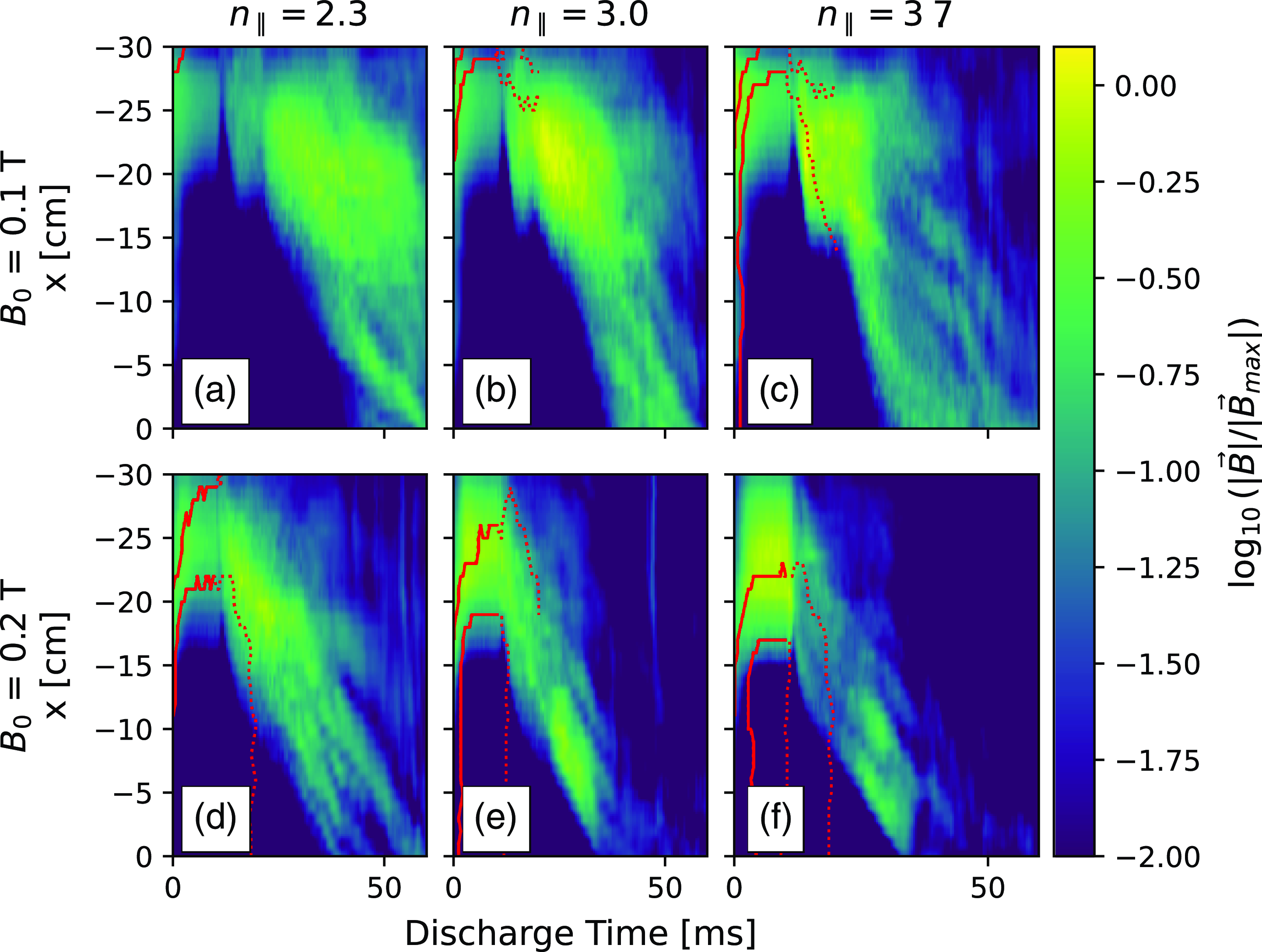
Figure 8. Measurements of the wave magnetic field from $\dot {B}$
probes. Overplotted is the contour of the region of accessible densities for the given combination of
$\dot {B}$
probes. Overplotted is the contour of the region of accessible densities for the given combination of $B_0$
and
$B_0$
and $n_\parallel$
.
$n_\parallel$
.
4. Mode identification
Here, we aim to identify and distinguish between the two cold-plasma modes the antenna could launch. The antenna is designed to predominantly excite the fast branch, as the current-carrying elements are aligned perpendicular to the static magnetic field and the resulting azimuthal wave electric field and axial wave magnetic field are well matched to the fast-wave polarization near the cutoff density. Verifying coupling to the fast mode thus demonstrates that the antenna does in fact behave as intended. There are several means by which we can distinguish the two branches. First, we can use the wave accessibility contours from § 3 to identify where both branches propagate. Within the contours we could measure both fast and slow waves, but at densities below the fast-wave cutoff density only slow waves can be observed. Next, we can note the separation in the perpendicular wavelengths of the wave modes as characterized in the dispersion relation, as shown in figure 3(a). For a given density away from the confluence density the fast branch is a much longer-wavelength mode, so measurements that show two propagating modes at different perpendicular length scales would suggest that the longer-wavelength mode corresponds to fast-wave excitation. Another distinguishing feature of the two branches is the orientation of the radial phase velocity relative to the group velocity. It is well known that the slow branch is a radially backward wave, so that the radial component of the group velocity and phase velocity are oppositely oriented (Pinsker Reference Pinsker2015). The fast branch is, by contrast, a forward wave. Since power must flow away from the antenna structure (causality) the parallel component of both the group and phase velocities are in the direction away from the antenna. It will be shown in § 4.1 that by comparing the orientation of the wave fronts in the XZ plane we can identify the forward and backward waves. By investigating each of these properties we can identify the wave mode present in the plasma for the extent of the parameter space explored in the experiments.
4.1. Wave front measurements
Measurements of the wave fronts in the XZ plane give us information about both the parallel and perpendicular structure of the propagating waves. A $\dot {B}$
probe is moved from shot to shot across the XZ plane, to each position within the data run plane. We then record 20 plasma shots at each position. These measurements were made over an area that spanned 20 cm in the z-direction and 40 cm in the x-direction with 1 cm resolution in each direction. The extent of the measurement domain restricted us from making reliable direct measurements in the change in the imposed parallel wavenumber spectrum. In order to recover the phase information of the wave fronts at each position we calculate the cross-spectrum between the antenna forward power and the respective component of the magnetic field measurement. This is mathematically equivalent to measuring the correlation between the two signals and maps out the phase and amplitude of the moving probe relative to the fixed reference phase of the antenna forward power. The spatial dependence of the relative phase results from the spatial structure of the wave, i.e. the wavenumber spectrum. From here we can work to identify the two modes. Figure 9 shows wave fronts measured for the nominal 476 MHz, 0.2 T case. The selected times shown are indicative of three distinct cases from the density contours in § 3: within the contour when the density is high enough to support fast-wave propagation, shortly after the density has dropped below the cutoff and late after the density is too low to support fast-wave propagation. Recall that the antenna is at x = −30 cm and z = 0 cm in our coordinate system. Waves launched from the antenna propagate away from the antenna structure, so the group velocity of the waves must be in the positive
$\dot {B}$
probe is moved from shot to shot across the XZ plane, to each position within the data run plane. We then record 20 plasma shots at each position. These measurements were made over an area that spanned 20 cm in the z-direction and 40 cm in the x-direction with 1 cm resolution in each direction. The extent of the measurement domain restricted us from making reliable direct measurements in the change in the imposed parallel wavenumber spectrum. In order to recover the phase information of the wave fronts at each position we calculate the cross-spectrum between the antenna forward power and the respective component of the magnetic field measurement. This is mathematically equivalent to measuring the correlation between the two signals and maps out the phase and amplitude of the moving probe relative to the fixed reference phase of the antenna forward power. The spatial dependence of the relative phase results from the spatial structure of the wave, i.e. the wavenumber spectrum. From here we can work to identify the two modes. Figure 9 shows wave fronts measured for the nominal 476 MHz, 0.2 T case. The selected times shown are indicative of three distinct cases from the density contours in § 3: within the contour when the density is high enough to support fast-wave propagation, shortly after the density has dropped below the cutoff and late after the density is too low to support fast-wave propagation. Recall that the antenna is at x = −30 cm and z = 0 cm in our coordinate system. Waves launched from the antenna propagate away from the antenna structure, so the group velocity of the waves must be in the positive $\hat {x}$
and positive
$\hat {x}$
and positive $\hat {z}$
direction pointing towards the bottom right of corner in each panel. For the high-density case we see a long-wavelength mode that spans the range
$\hat {z}$
direction pointing towards the bottom right of corner in each panel. For the high-density case we see a long-wavelength mode that spans the range $-25$
cm
$-25$
cm $\leqslant x \leqslant -12.5$
cm. The radial (
$\leqslant x \leqslant -12.5$
cm. The radial ( $\hat {x}$
-direction) component of the phase velocity of this mode is in the positive x-direction, suggesting that the mode is a forward-propagating mode or fast-wave-like. We can contrast this with the late discharge time measurement that show wave fronts with an oppositely oriented radial phase velocity. This mode also has a much shorter perpendicular length scale. The combination of low-density propagation, backward phase velocity and short wavelength all support that at late discharge times we are measuring a propagating slow wave. Hence, for a given static magnetic field and
$\hat {x}$
-direction) component of the phase velocity of this mode is in the positive x-direction, suggesting that the mode is a forward-propagating mode or fast-wave-like. We can contrast this with the late discharge time measurement that show wave fronts with an oppositely oriented radial phase velocity. This mode also has a much shorter perpendicular length scale. The combination of low-density propagation, backward phase velocity and short wavelength all support that at late discharge times we are measuring a propagating slow wave. Hence, for a given static magnetic field and $n_\parallel$
, at low enough densities the antenna directly excites the slow mode. A visual interpretation of the intermediate case is not as straightforward. A combination of modes exist in this case as well as a clearer dependence on the density profile for the wavelength of the slow branch. Section 4.2 will show calculations of the perpendicular wavenumber compared with measurements of the
$n_\parallel$
, at low enough densities the antenna directly excites the slow mode. A visual interpretation of the intermediate case is not as straightforward. A combination of modes exist in this case as well as a clearer dependence on the density profile for the wavelength of the slow branch. Section 4.2 will show calculations of the perpendicular wavenumber compared with measurements of the $\hat {x}$
-component wavenumber from the XZ planes show in this section. From this we can see a clear delineation of the modes from the magnitude and sign of the measured
$\hat {x}$
-component wavenumber from the XZ planes show in this section. From this we can see a clear delineation of the modes from the magnitude and sign of the measured $k_x$
.
$k_x$
.
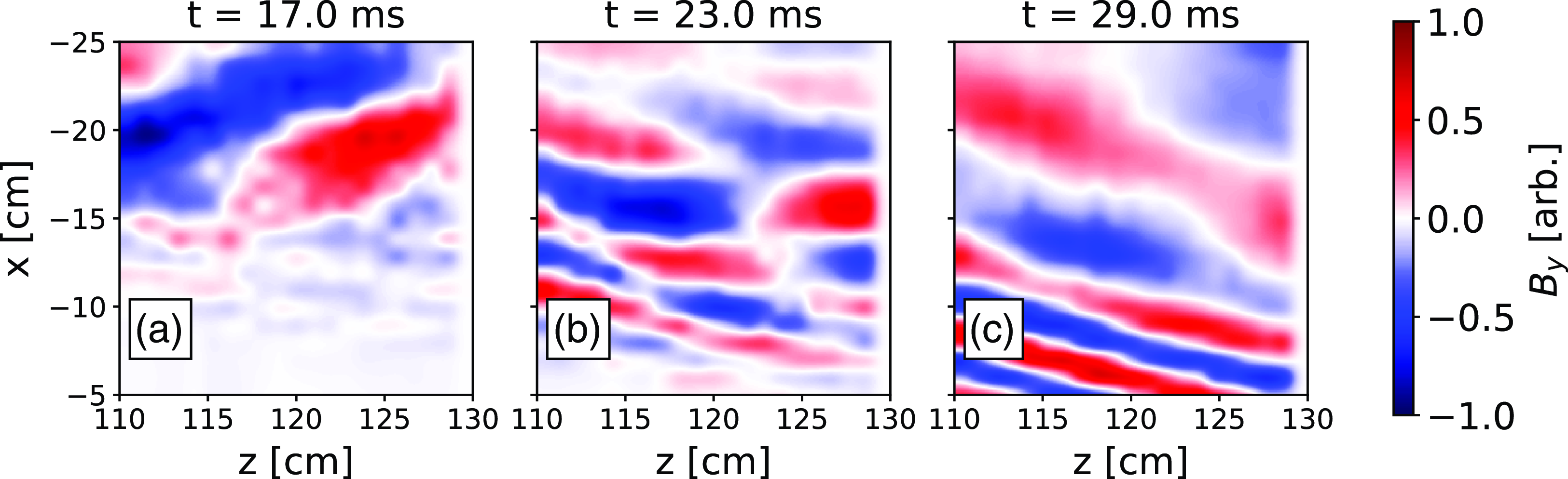
Figure 9. Cross-spectrum measurements of the y-component of the wave magnetic field in the XZ plane for the 476 MHz, 0.2 T case. Discharge time is used as a proxy for density here; increasing discharge time corresponds to lower densities. (a) High-density case in the early afterglow t = 17 ms. (b) Intermediate discharge time, t = 23 ms. (c) Late afterglow, t = 29 ms.
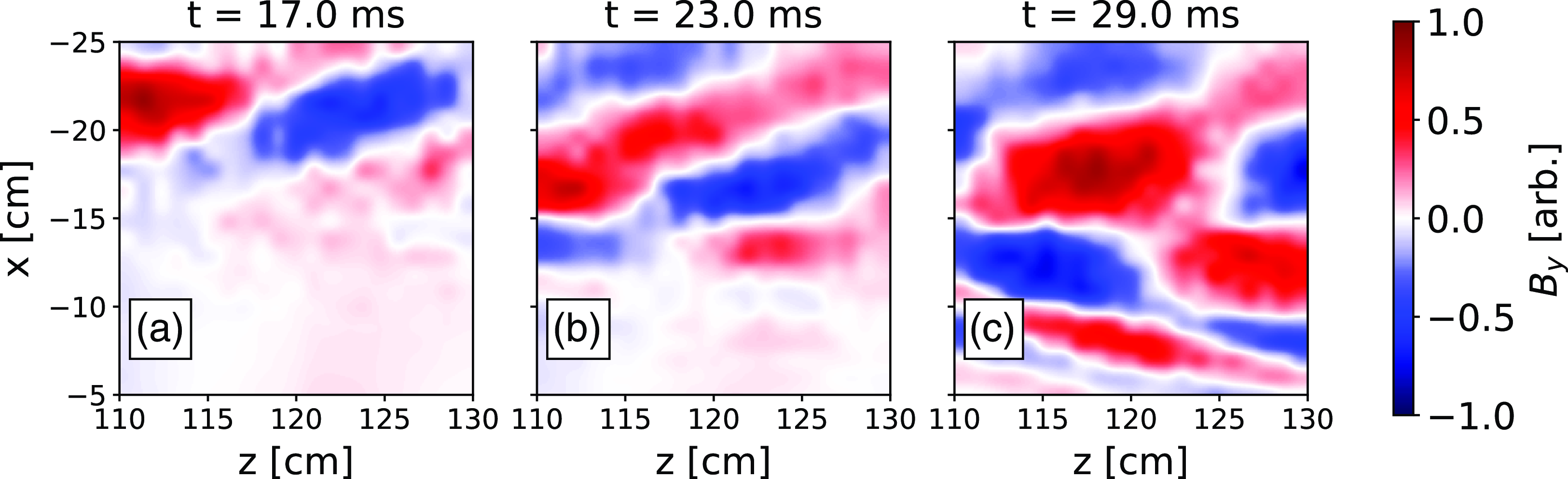
Figure 10. Cross-spectrum measurements of the y-component of the wave magnetic field in the XZ plane for the 466 MHz, 0.2 T case. (a) High-density case in the early afterglow t = 17 ms. (b) Intermediate discharge time, t = 23 ms. (c) Late afterglow, t = 29 ms.
Figure 10 shows the lower frequency case. At lower drive frequency on the antenna we expect a lower launched $n_\parallel$
; for 466 MHz we estimate
$n_\parallel$
; for 466 MHz we estimate $n_\parallel \approx 2.3$
from the measured phase jump between adjacent modules. With a lower launch
$n_\parallel \approx 2.3$
from the measured phase jump between adjacent modules. With a lower launch $n_\parallel$
the fast-wave cutoff density is reduced, so we expect that fast-wave propagation should occur at later discharge times. This is seen in figure 10 where panels (a) and (b) clearly both show the long-wavelength forward wave mode. In panel (c) we see a combination of modes as even at the late discharge time the density is still high enough to support fast-wave propagation.
$n_\parallel$
the fast-wave cutoff density is reduced, so we expect that fast-wave propagation should occur at later discharge times. This is seen in figure 10 where panels (a) and (b) clearly both show the long-wavelength forward wave mode. In panel (c) we see a combination of modes as even at the late discharge time the density is still high enough to support fast-wave propagation.
4.2. Comparison with the cold-plasma dispersion relationship
A comparison with the cold-plasma dispersion relationship can be made for each case. Using the static magnetic field, predicted imposed parallel wavelength and line-averaged density, we compute the perpendicular wavenumber ( $k_\perp$
) for both cold-plasma branches as a function of density. From the wavefront images in § 4.1 we take the spatial Fourier transform to extract the
$k_\perp$
) for both cold-plasma branches as a function of density. From the wavefront images in § 4.1 we take the spatial Fourier transform to extract the $\hat {x}$
-component of the wavenumber spectrum as a function of discharge time. Matching the discharge time to the line-averaged density, we can see significant overlap in the predicted spectrum with the measured spectrum from the experiments. Figure 11 shows this for the nominal 476 MHz,
$\hat {x}$
-component of the wavenumber spectrum as a function of discharge time. Matching the discharge time to the line-averaged density, we can see significant overlap in the predicted spectrum with the measured spectrum from the experiments. Figure 11 shows this for the nominal 476 MHz, $B_0$
= 0.2 T case. We can see that there are clearly two branches present in the measurement, as expected from the calculation using the cold-plasma dispersion relationship. At earlier discharge times we see that the plasma supports both the fast and slow branches for the given set of antenna and plasma parameters. As the discharge progresses and the density drops, the fast-wave branch decreases in wavenumber (increases in wavelength), as seen both in the expected
$B_0$
= 0.2 T case. We can see that there are clearly two branches present in the measurement, as expected from the calculation using the cold-plasma dispersion relationship. At earlier discharge times we see that the plasma supports both the fast and slow branches for the given set of antenna and plasma parameters. As the discharge progresses and the density drops, the fast-wave branch decreases in wavenumber (increases in wavelength), as seen both in the expected $k_\perp$
and in the measurements. Throughout the discharge we see an oppositely signed
$k_\perp$
and in the measurements. Throughout the discharge we see an oppositely signed $k_x$
that follows the expected
$k_x$
that follows the expected $k_\perp$
for the slow branch. Figure 12 shows this comparison for four cases: (a) 466 MHz and
$k_\perp$
for the slow branch. Figure 12 shows this comparison for four cases: (a) 466 MHz and $B_0$
= 0.1 T, (b) 486 MHz and
$B_0$
= 0.1 T, (b) 486 MHz and $B_0$
= 0.1 T, (c) 466 MHz and
$B_0$
= 0.1 T, (c) 466 MHz and $B_0$
= 0.2 T, (d) 486 MHz and
$B_0$
= 0.2 T, (d) 486 MHz and $B_0$
= 0.2 T. Again, we see good agreement between the expected
$B_0$
= 0.2 T. Again, we see good agreement between the expected $k_\perp$
and measured
$k_\perp$
and measured $k_x$
for each case. Each case demonstrates two branches with oppositely signed
$k_x$
for each case. Each case demonstrates two branches with oppositely signed $k_x$
which have correspondingly separated length scales. However, since we are using the line-averaged density to compare with our measured spectrum we note that there should be significant spread in the measured spectrum due to the fact that our plasma is not uniform in density across the whole column. The non-uniform density gives rise to a range of wavelengths. Additionally, this does not capture the spatial profiles of the waves. For example, figure 12(a) shows wave power at discharge times before the line-averaged density would suggest the plasma supports wave propagation. Further investigation of this case shows that the waves are only in the edge of the plasma, where the density is low enough to support wave propagation. At later times where the line-averaged density suggests waves may propagate we see that the waves are measured in the bulk of the plasma rather than only in the edge. Although there may be some discrepancy between the measured onset of fast-wave propagation and what is predicted using the line-averaged density, the trend in relation to the change in the imposed parallel wavenumber matches well. This shows that we are able to vary the imposed parallel wavenumber by changing the antenna drive frequency, as intended. Further, it demonstrates that the antenna does launch fast waves as intended when the plasma supports fast-wave propagation. However, it also shows that there is direct coupling to the slow mode for plasma conditions in which the density is too low for fast-wave propagation. It is important to point out that, although figures 11 and 12 show little to no power in the wavenumber spectrum at the early discharge times, there were in fact significant levels of wave power measured. During the powered portion of the discharge,
$k_x$
which have correspondingly separated length scales. However, since we are using the line-averaged density to compare with our measured spectrum we note that there should be significant spread in the measured spectrum due to the fact that our plasma is not uniform in density across the whole column. The non-uniform density gives rise to a range of wavelengths. Additionally, this does not capture the spatial profiles of the waves. For example, figure 12(a) shows wave power at discharge times before the line-averaged density would suggest the plasma supports wave propagation. Further investigation of this case shows that the waves are only in the edge of the plasma, where the density is low enough to support wave propagation. At later times where the line-averaged density suggests waves may propagate we see that the waves are measured in the bulk of the plasma rather than only in the edge. Although there may be some discrepancy between the measured onset of fast-wave propagation and what is predicted using the line-averaged density, the trend in relation to the change in the imposed parallel wavenumber matches well. This shows that we are able to vary the imposed parallel wavenumber by changing the antenna drive frequency, as intended. Further, it demonstrates that the antenna does launch fast waves as intended when the plasma supports fast-wave propagation. However, it also shows that there is direct coupling to the slow mode for plasma conditions in which the density is too low for fast-wave propagation. It is important to point out that, although figures 11 and 12 show little to no power in the wavenumber spectrum at the early discharge times, there were in fact significant levels of wave power measured. During the powered portion of the discharge, $0\leqslant t_{\mathrm{dis}} \leqslant 10$
ms, wave power was measured in the plasma edge but we were unable to discern the structure using the methods described here. This is most likely due to drift waves in the plasma edge during the powered phase of the discharge, during which the strong drift mode activity creates a time-varying coupling and propagation region for the waves in the edge. This incoherent shot-to-shot variation prohibits us from gathering meaningful phase information. We also note that wave power was measured in the case 466 MHz,
$0\leqslant t_{\mathrm{dis}} \leqslant 10$
ms, wave power was measured in the plasma edge but we were unable to discern the structure using the methods described here. This is most likely due to drift waves in the plasma edge during the powered phase of the discharge, during which the strong drift mode activity creates a time-varying coupling and propagation region for the waves in the edge. This incoherent shot-to-shot variation prohibits us from gathering meaningful phase information. We also note that wave power was measured in the case 466 MHz, $B_0$
= 0.1 T case during
$B_0$
= 0.1 T case during $20\leqslant t_{\mathrm{dis}} \leqslant 40$
ms, well into the afterglow of the discharge where drift modes are less prevalent. We are not able to measure the
$20\leqslant t_{\mathrm{dis}} \leqslant 40$
ms, well into the afterglow of the discharge where drift modes are less prevalent. We are not able to measure the $k_x$
spectrum here, possibly due to the fact that the plasma density is well above the confluence density for the principal imposed
$k_x$
spectrum here, possibly due to the fact that the plasma density is well above the confluence density for the principal imposed $n_\parallel$
so waves would propagate in and mode convert to propagate back out as a slow wave. This process could lead to interference and a complicated wave front pattern that is not discernible in the measurements.
$n_\parallel$
so waves would propagate in and mode convert to propagate back out as a slow wave. This process could lead to interference and a complicated wave front pattern that is not discernible in the measurements.
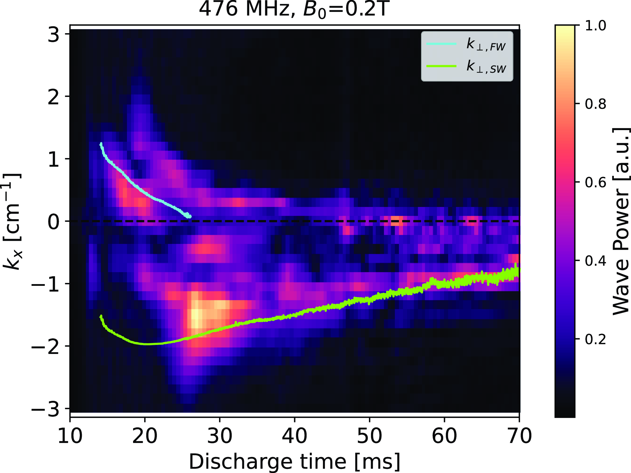
Figure 11. Comparison of measured $k_x$
spectrum with calculated cold-plasma dispersion
$k_x$
spectrum with calculated cold-plasma dispersion $k_\perp$
for both cold-plasma branches at 476 MHz and
$k_\perp$
for both cold-plasma branches at 476 MHz and $B_0$
= 0.2 T.
$B_0$
= 0.2 T.
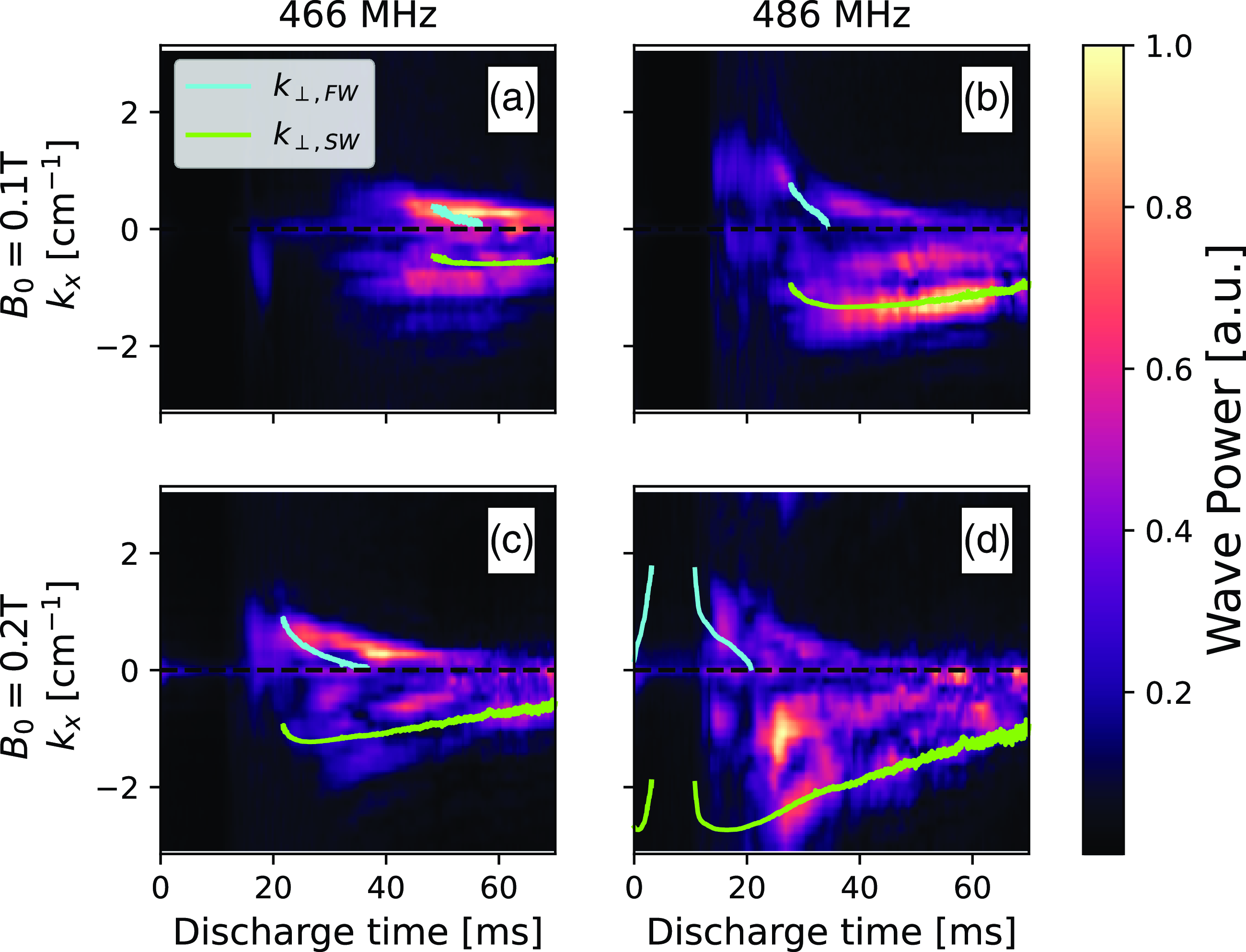
Figure 12. Comparison of measured $k_x$
spectrum with calculated cold-plasma dispersion
$k_x$
spectrum with calculated cold-plasma dispersion $k_\perp$
for both cold-plasma branches for: (a) 466 MHz, 0.1 T; (b) 486 MHz, 0.1 T; (c) 466 MHz, 0.2 T; (d) 486 MHz, 0.2 T.
$k_\perp$
for both cold-plasma branches for: (a) 466 MHz, 0.1 T; (b) 486 MHz, 0.1 T; (c) 466 MHz, 0.2 T; (d) 486 MHz, 0.2 T.
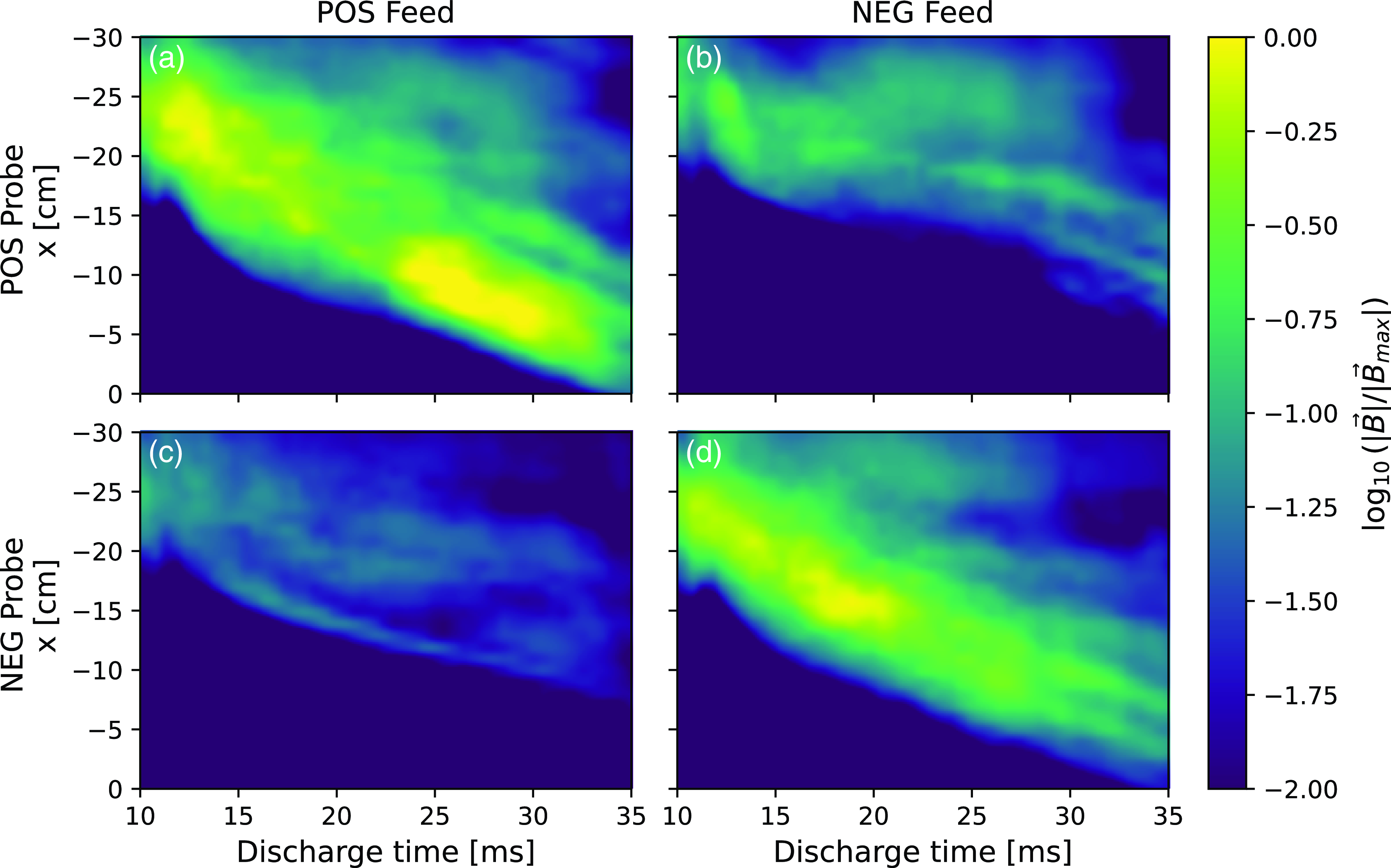
Figure 13. Comparison of wave magnetic fields as measured by $\dot {B}$
probes when exchanging antenna feed side; the left column shows the POS side launch feed case and the right column shows the NEG side launch feed case.
$\dot {B}$
probes when exchanging antenna feed side; the left column shows the POS side launch feed case and the right column shows the NEG side launch feed case.
5. Directionality measurements
In this section we aim to demonstrate the directional launch capabilities of the TWA. Launch direction is set by which end of the antenna array is directly fed by the RF source. From the feed module, power is inductively coupled into the subsequent modules. The direction of energy flow corresponds to the direction of the wave launch or the direction of the $n_\parallel$
excited by the antenna. The
$n_\parallel$
excited by the antenna. The $\dot {B}$
probes were stationed on ports separated from the center of the antenna array by 1.2 m, with one probe stationed on either side of the antenna array. Comparing the signals measured on either side of the antenna as the launch direction is exchanged is a clear indicator of whether the antenna is able to preferentially excite the intended sign of
$\dot {B}$
probes were stationed on ports separated from the center of the antenna array by 1.2 m, with one probe stationed on either side of the antenna array. Comparing the signals measured on either side of the antenna as the launch direction is exchanged is a clear indicator of whether the antenna is able to preferentially excite the intended sign of $n_\parallel$
. Shown in figure 13 are measurements of the amplitude of the magnetic field measured by these probes at the RF frequency. The probe signals are normalized by the peak signal measured on the probe between the two cases. Here, we are operating the antenna in the nominal case:
$n_\parallel$
. Shown in figure 13 are measurements of the amplitude of the magnetic field measured by these probes at the RF frequency. The probe signals are normalized by the peak signal measured on the probe between the two cases. Here, we are operating the antenna in the nominal case: $f_0$
= 476 MHz,
$f_0$
= 476 MHz, $n_\parallel$
= 3.0 and
$n_\parallel$
= 3.0 and $B_0$
= 0.2 T. Figure 13 shows the fields measured when launching in what we denote as the positive direction (POS). It is clear that the amplitude of the measured fields is much larger on the positive side of the antenna – almost an order of magnitude difference at a given time during the discharge. There are some non-zero fields that are measured on the opposite side of the antenna. This is expected as the antenna spectrum is not 100
$B_0$
= 0.2 T. Figure 13 shows the fields measured when launching in what we denote as the positive direction (POS). It is clear that the amplitude of the measured fields is much larger on the positive side of the antenna – almost an order of magnitude difference at a given time during the discharge. There are some non-zero fields that are measured on the opposite side of the antenna. This is expected as the antenna spectrum is not 100 $\%$
directional. The same can be seen when the feed side is exchanged, where the right column of figure 13 is for the negative feed side (NEG). The amplitudes of the measured fields change accordingly, that is, higher amplitudes are measured on the negative side of the antenna when the antenna is fed for negative side launch. The clear difference in measured magnetic field amplitude shows that the antenna operates as intended when exchanging feed sides. This demonstrates that the TWA does exhibit directional launch in the LAPD.
$\%$
directional. The same can be seen when the feed side is exchanged, where the right column of figure 13 is for the negative feed side (NEG). The amplitudes of the measured fields change accordingly, that is, higher amplitudes are measured on the negative side of the antenna when the antenna is fed for negative side launch. The clear difference in measured magnetic field amplitude shows that the antenna operates as intended when exchanging feed sides. This demonstrates that the TWA does exhibit directional launch in the LAPD.
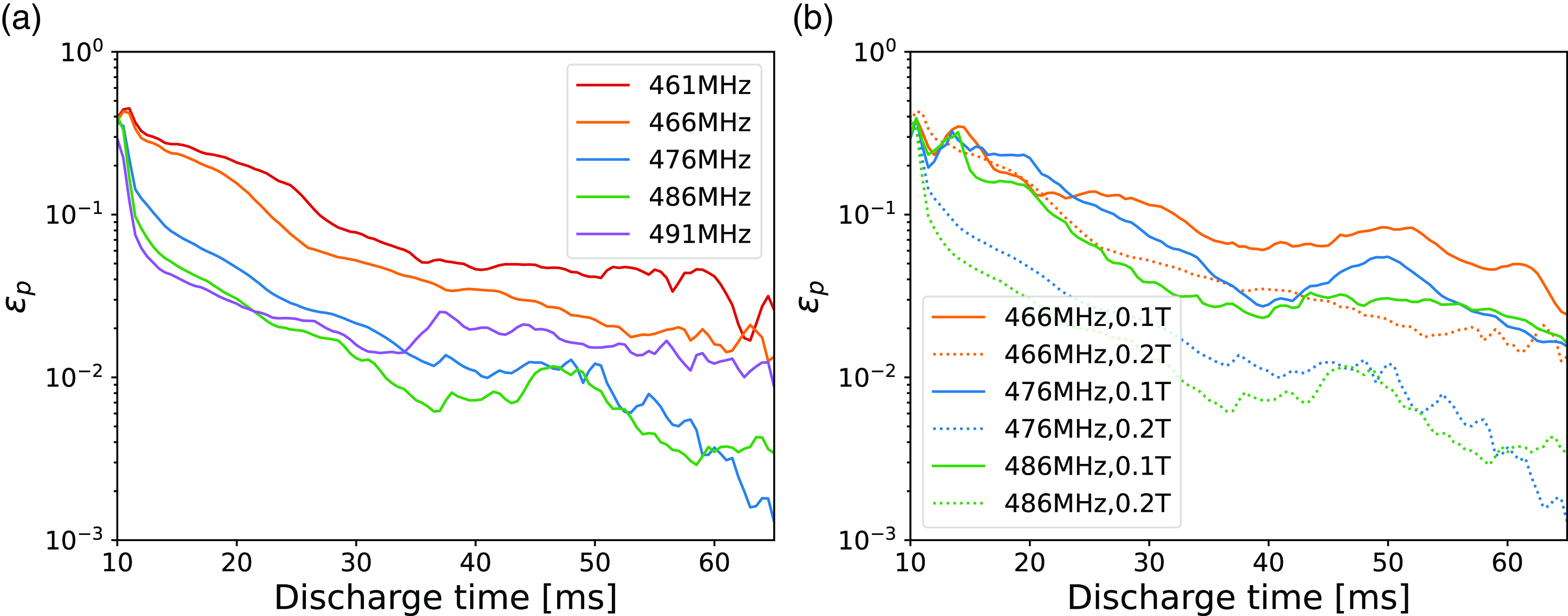
Figure 14. Loading measurements: (a) scanned over frequency for $B_0$
= 0.2 T, (b) scanned over magnetic field at different frequencies.
$B_0$
= 0.2 T, (b) scanned over magnetic field at different frequencies.
6. Antenna loading
Here, we investigate the effects of static magnetic field, density and launched $n_\parallel$
on antenna loading. Antenna loading is characterized as the decay in the measured fields along the antenna array. Power is coupled into the feed module of the antenna array, a fraction of the power is radiated into the plasma with the remaining power coupling into the next module through mutual inductance. Each module radiates some power and couples the residual amount to the subsequent module (except the end module in which residual power is fed into a 50
$n_\parallel$
on antenna loading. Antenna loading is characterized as the decay in the measured fields along the antenna array. Power is coupled into the feed module of the antenna array, a fraction of the power is radiated into the plasma with the remaining power coupling into the next module through mutual inductance. Each module radiates some power and couples the residual amount to the subsequent module (except the end module in which residual power is fed into a 50 $\varOmega$
dummy load). By measuring the magnetic fields at each antenna module and calculating the rate of decay of the fields along the array we can quantify the loading of the antenna due to the plasma by comparison with the vacuum (unloaded) case. Faster rates of decay along the array corresponds to higher loading, with the quantity
$\varOmega$
dummy load). By measuring the magnetic fields at each antenna module and calculating the rate of decay of the fields along the array we can quantify the loading of the antenna due to the plasma by comparison with the vacuum (unloaded) case. Faster rates of decay along the array corresponds to higher loading, with the quantity $\epsilon _p$
being used to denote this decay in fields along the array due to coupling to the plasma. Figure 14(a) shows a frequency scan at the nominal 0.2 T static magnetic field, the scan in frequency corresponding to a scan of
$\epsilon _p$
being used to denote this decay in fields along the array due to coupling to the plasma. Figure 14(a) shows a frequency scan at the nominal 0.2 T static magnetic field, the scan in frequency corresponding to a scan of $n_\parallel$
. There is a clear trend in the drop in loading as the plasma density decreases, noting that later discharge times correspond to lower line-averaged densities. We can see that as the frequency applied to the antenna increases the plasma loading on the antenna decreases. This can be attributed to the increase in the imposed
$n_\parallel$
. There is a clear trend in the drop in loading as the plasma density decreases, noting that later discharge times correspond to lower line-averaged densities. We can see that as the frequency applied to the antenna increases the plasma loading on the antenna decreases. This can be attributed to the increase in the imposed $n_\parallel$
shifting the fast-wave cutoff density to higher density, so that the region which supports fast-wave propagation in the plasma becomes small or non-existent, as can be seen in the contours drawn on figure 7. In contrast, we see that the loading on the antenna is high for the 461 and 466 MHz cases. The contours in figure 7 suggest that, for the 466 MHz case, the fast-wave cutoff density reaches all the way to the antenna face. A comparison with the measured wave fields, shown in figure 10, demonstrate that at the time in which we see high loading we do in fact see fast-wave propagation. However, we also observe that the loading drops while the plasma does support fast-wave propagation at discharge times
$n_\parallel$
shifting the fast-wave cutoff density to higher density, so that the region which supports fast-wave propagation in the plasma becomes small or non-existent, as can be seen in the contours drawn on figure 7. In contrast, we see that the loading on the antenna is high for the 461 and 466 MHz cases. The contours in figure 7 suggest that, for the 466 MHz case, the fast-wave cutoff density reaches all the way to the antenna face. A comparison with the measured wave fields, shown in figure 10, demonstrate that at the time in which we see high loading we do in fact see fast-wave propagation. However, we also observe that the loading drops while the plasma does support fast-wave propagation at discharge times $t_{\mathrm{dis}}\gt 25$
ms. It is unclear how to distinguish the difference in increased evanescence and the decrease in the line-averaged density. We note that the loading is significantly higher when we measure fast-wave propagation, up to
$t_{\mathrm{dis}}\gt 25$
ms. It is unclear how to distinguish the difference in increased evanescence and the decrease in the line-averaged density. We note that the loading is significantly higher when we measure fast-wave propagation, up to $\sim 3\times$
larger for the 466 MHz case during discharge times that support fast-wave propagation than in the late discharge times that support only slow-wave propagation. Similarly, figure 14(b) shows higher loading throughout much of the discharge for the 466 MHz,
$\sim 3\times$
larger for the 466 MHz case during discharge times that support fast-wave propagation than in the late discharge times that support only slow-wave propagation. Similarly, figure 14(b) shows higher loading throughout much of the discharge for the 466 MHz, $B_0$
= 0.1 T case where we measured fast-wave propagation. The scan in magnetic field shows that the antenna loading is higher in the low-field case for later times in the discharge. The decrease in static magnetic field corresponds to a decrease in the fast-wave cutoff density for a given value of
$B_0$
= 0.1 T case where we measured fast-wave propagation. The scan in magnetic field shows that the antenna loading is higher in the low-field case for later times in the discharge. The decrease in static magnetic field corresponds to a decrease in the fast-wave cutoff density for a given value of $n_\parallel$
, so we expect that the higher loading in the low-field cases at low density corresponds to coupling to the fast wave. This can be seen in the comparison with the dispersion relation plots in figure 12, where we see significant power in the fast-wave branch at discharge times where we see high loading.
$n_\parallel$
, so we expect that the higher loading in the low-field cases at low density corresponds to coupling to the fast wave. This can be seen in the comparison with the dispersion relation plots in figure 12, where we see significant power in the fast-wave branch at discharge times where we see high loading.
7. Comparison with modeling
A series of modeling efforts were made to support the analysis of the results of these experiments. An axisymmetric cold-plasma model was used to understand the excitation of both cold-plasma modes in an LAPD-like plasma. The model uses density profiles that are representative of the experiments. Although the antenna is not axisymmetric, we can use the results of the model to gain insight into the observation of two cold-plasma modes in the experiment. Further work was conducted using the code RFPisa from TAE Technologies. Our experiments served as a means for validating the RFPisa code in a simple geometry.
7.1. Full-wave axisymmetric cold-plasma model
To gain an understanding of the modes present at a given density we aimed to create a simple model of our experiment. While the previous sections have shown, through comparison with the cold-plasma dispersion relationship, the presence of each mode, this additional step to demonstrate the measured wave fields are in fact the corresponding branch ensures that geometric effects or reflections are not responsible for the resulting wave patterns. Within the model we can see that the measured fields are a result of the directly launched wave from the antenna structure.
A finite element method (FEM) solver, COMSOL Multiphysics (AB, 2024), was used to solve the wave equation in a cold plasma with density profiles similar to our experiment. The model uses a cylindrical LAPD-like plasma in a two-dimensional axisymmetric geometry. Cylindrical coordinates are used: $\vec{r}=(r,\phi,z)$
. We assume symmetry about the center axis of the LAPD vessel such that the quantities have the following dependence:
$\vec{r}=(r,\phi,z)$
. We assume symmetry about the center axis of the LAPD vessel such that the quantities have the following dependence:
 \begin{equation} \boldsymbol{E}(r,\phi ,z) = \boldsymbol{E}(r,z)e^{im\phi } ,\end{equation}
where $m$
is the azimuthal mode number. The FEM solver then solves the following equation for the wave electric field:
$m$
is the azimuthal mode number. The FEM solver then solves the following equation for the wave electric field:
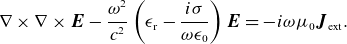 \begin{equation} \nabla \times \nabla \times \boldsymbol{E} - \frac {\omega ^2}{c^2}\left({\epsilon _{\mathrm{ r}}}-\frac {i{\sigma }}{\omega \epsilon _0}\right)\boldsymbol{E}= -i\omega \mu _0\boldsymbol{J}_{\mathrm{ext}}. \end{equation}
Although the antenna’s finite vertical extent breaks the axisymmetry we can use the model to understand how the azimuthal modes contribute to excite the fast and slow branches. To model the antenna, we used a series of current-carrying rings set at the antenna radius. Phasing between the rings, $\delta _{\mathrm{n}}$
, can be changed to set the imposed parallel wavelength or
$\delta _{\mathrm{n}}$
, can be changed to set the imposed parallel wavelength or $n_\parallel$
. Additionally, a decay factor,
$n_\parallel$
. Additionally, a decay factor, $\beta$
, represents the decay in module power along the current-carrying rings that can be set to account for antenna loading, this being equivalent to the
$\beta$
, represents the decay in module power along the current-carrying rings that can be set to account for antenna loading, this being equivalent to the $\epsilon _p$
quantity from § 6. The total external current is
$\epsilon _p$
quantity from § 6. The total external current is
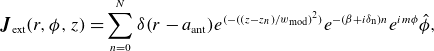 \begin{equation} \boldsymbol{J}_{\mathrm{ext}}(r,\phi ,z) = \sum _{n=0}^{N}\delta (r-a_{\mathrm{ant}})e^{(-((z-z_n)/w_{\mathrm{mod}})^2)}e^{-(\beta +i\delta _{\mathrm{ n}})n}e^{im\phi }\hat {\phi } ,\end{equation}
where n is the module number, N is the total number of modules, $\delta (r)$
is the Dirac delta function,
$\delta (r)$
is the Dirac delta function, $a_{\mathrm{ant}}$
is the antenna position radius,
$a_{\mathrm{ant}}$
is the antenna position radius, $z_{\mathrm{n}}$
is the module position along the array and
$z_{\mathrm{n}}$
is the module position along the array and $w_{\mathrm{ mod}}$
is the field parallel length scale of the current-carrying element in the module. Density profiles in the model take the form
$w_{\mathrm{ mod}}$
is the field parallel length scale of the current-carrying element in the module. Density profiles in the model take the form
 \begin{equation} n_{\mathrm{e}}(r) = n_0(1-\tanh {((r/a_{\mathrm{plasma}})^4)}). \end{equation}
The parameter $n_0$
is used to adjust the peak density as measured in the experiment and
$n_0$
is used to adjust the peak density as measured in the experiment and $a_{plasma}$
is used to adjust the profile width. This profile is essentially flat around the center, but captures the density gradient in the edge. An artificial conductivity
$a_{plasma}$
is used to adjust the profile width. This profile is essentially flat around the center, but captures the density gradient in the edge. An artificial conductivity $\sigma$
is imposed at the edges of the simulation domain to damp the waves as there was little evidence of significant end reflections in our experimental data set. For all of the following figures, an m-number of
$\sigma$
is imposed at the edges of the simulation domain to damp the waves as there was little evidence of significant end reflections in our experimental data set. For all of the following figures, an m-number of $m=6$
was chosen. While we do not expect the antenna to excite a single m-number, a selection
$m=6$
was chosen. While we do not expect the antenna to excite a single m-number, a selection $m=6$
is justified in that the antenna’s vertical extent subtends
$m=6$
is justified in that the antenna’s vertical extent subtends $\sim 1/6$
of the plasma circumference. From here we will discuss the comparison of the model results with the experiment.
$\sim 1/6$
of the plasma circumference. From here we will discuss the comparison of the model results with the experiment.
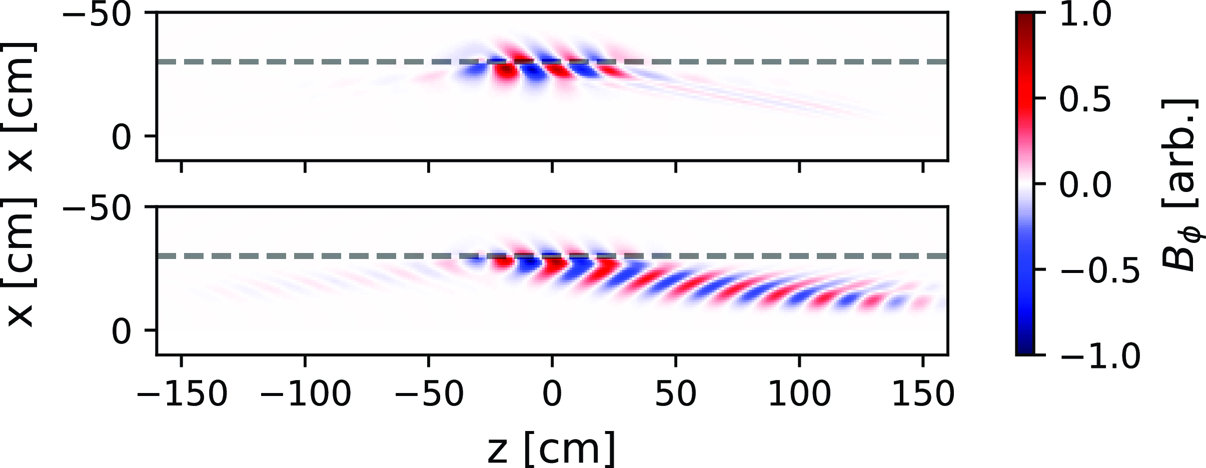
Figure 15. Full domain of COMSOL model run using nominal 476 MHz, $B_0$
= 0.2 T case,
$B_0$
= 0.2 T case, $m=6$
. Densities are representative of timings in figure 9:
$m=6$
. Densities are representative of timings in figure 9: $n_0=1.5\times 10^{17}$
(m
$n_0=1.5\times 10^{17}$
(m $^{-3}$
) (top),
$^{-3}$
) (top), $n_0=5.5\times 10^{17}$
(m
$n_0=5.5\times 10^{17}$
(m $^{-3}$
) (bottom).
$^{-3}$
) (bottom).
Figure 15 shows the wave fields within the entire simulation domain for two density cases: $n_0=1.5\times 10^{17}$
(m
$n_0=1.5\times 10^{17}$
(m $^{-3}$
) and
$^{-3}$
) and $n_0=5.5\times 10^{17}$
(m
$n_0=5.5\times 10^{17}$
(m $^{-3}$
) in the nominal antenna configuration of
$^{-3}$
) in the nominal antenna configuration of $f_0=476$
MHz,
$f_0=476$
MHz, $B_0 = 0.2$
T. The antenna is centered at
$B_0 = 0.2$
T. The antenna is centered at $z=0$
cm and
$z=0$
cm and $r=30$
cm. We can immediately see that waves are launched with a preferential direction from the antenna. Using the nominal 476 MHz,
$r=30$
cm. We can immediately see that waves are launched with a preferential direction from the antenna. Using the nominal 476 MHz, $B_0$
= 0.2 T case, figure 16 shows the wave fields in the region where we took measurements during the experiments. The three panels show wave fronts for density profiles that are representative of times during the discharge shown in figure 9. We can see in Figure 16(a) that the long-wavelength forward-propagating mode is present as it was in the experimental data. At a lower density/later discharge time, figure 16(b), the wave front pattern become more complicated as a combination of modes is present. At low density/late discharge time, figure 16(c), the long-wavelength forward-propagating mode is no longer present, only a shorter backward-propagating mode can be seen. This agrees well with what was measured experimentally.
$B_0$
= 0.2 T case, figure 16 shows the wave fields in the region where we took measurements during the experiments. The three panels show wave fronts for density profiles that are representative of times during the discharge shown in figure 9. We can see in Figure 16(a) that the long-wavelength forward-propagating mode is present as it was in the experimental data. At a lower density/later discharge time, figure 16(b), the wave front pattern become more complicated as a combination of modes is present. At low density/late discharge time, figure 16(c), the long-wavelength forward-propagating mode is no longer present, only a shorter backward-propagating mode can be seen. This agrees well with what was measured experimentally.
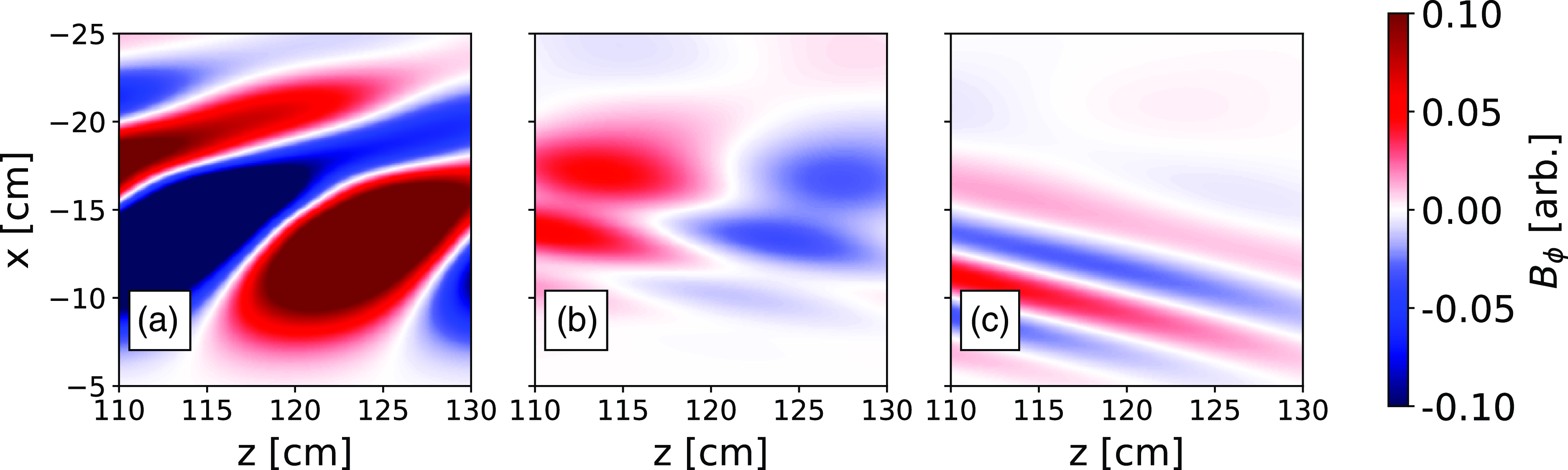
Figure 16. The COMSOL model run using nominal 476 MHz, $B_0$
= 0.2 T case,
$B_0$
= 0.2 T case, $m=6$
. Densities are representative of timings in corresponding panels of figure 9: (a)
$m=6$
. Densities are representative of timings in corresponding panels of figure 9: (a) $n_0=5.5\times 10^{17}$
(m
$n_0=5.5\times 10^{17}$
(m $^{-3}$
), (b)
$^{-3}$
), (b) $n_0=2.5\times 10^{17}$
(m
$n_0=2.5\times 10^{17}$
(m $^{-3}$
), (c)
$^{-3}$
), (c) $n_0=1.5\times 10^{17}$
(m
$n_0=1.5\times 10^{17}$
(m $^{-3}$
).
$^{-3}$
).
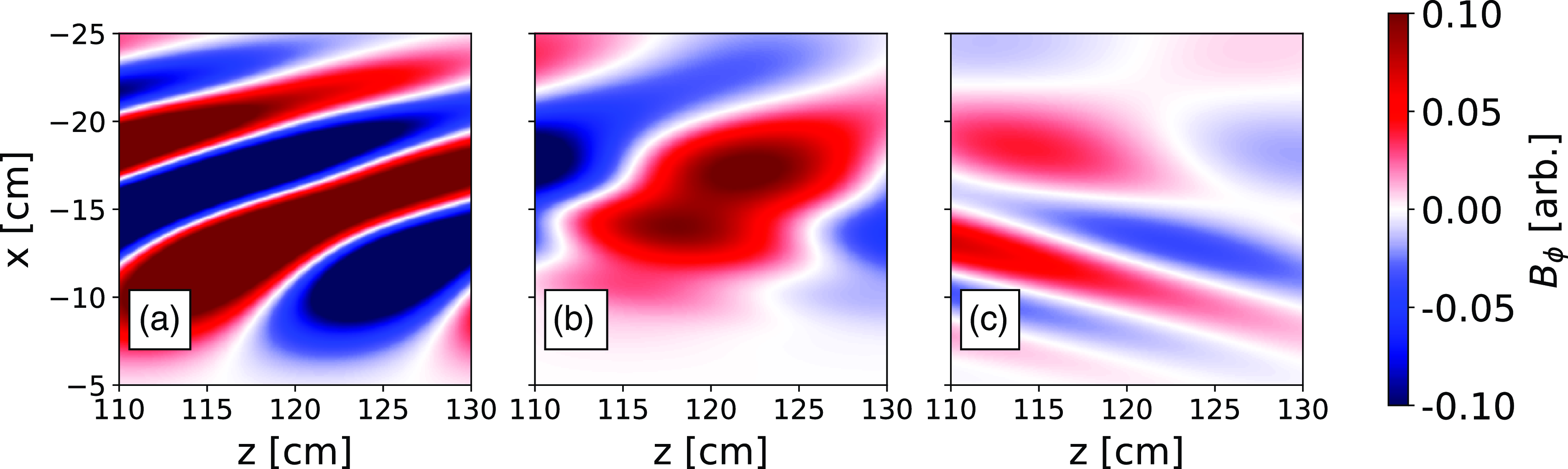
Figure 17. The COMSOL model run using 466 MHz, $B_0$
= 0.2T case,
$B_0$
= 0.2T case, $m=6$
. Densities are representative of timings in corresponding panels of figure 10: (a)
$m=6$
. Densities are representative of timings in corresponding panels of figure 10: (a) $n_0=5.5\times 10^{17}$
(m
$n_0=5.5\times 10^{17}$
(m $^{-3}$
), (b)
$^{-3}$
), (b) $n_0=2.5\times 10^{17}$
(m
$n_0=2.5\times 10^{17}$
(m $^{-3}$
), (c)
$^{-3}$
), (c) $n_0=1.5\times 10^{17}$
(m
$n_0=1.5\times 10^{17}$
(m $^{-3}$
).
$^{-3}$
).
Figure 17 shows the same section of the simulation domain with the parameters adjusted to reflect the antenna being run at 466 MHz. This involves adjusting the phasing between the current rings to excite an $n_\parallel \approx 2.3$
. At this lower antenna frequency and imposed
$n_\parallel \approx 2.3$
. At this lower antenna frequency and imposed $n_\parallel$
we see that the perpendicular wavelength in the high-density case, figure 17(a), is shorter than the 476 MHz case, as expected from the dispersion relationship and in agreement with what was measured in the experiment. In the intermediate density case, the long-wavelength forward-propagating mode is still present but with a longer perpendicular wavelength as expected from the dispersion relationship. Lastly, the low-density case shows only the slow mode in the core with some evidence of an edge mode present. Again these panels agree well with what was measured in the experiment.
$n_\parallel$
we see that the perpendicular wavelength in the high-density case, figure 17(a), is shorter than the 476 MHz case, as expected from the dispersion relationship and in agreement with what was measured in the experiment. In the intermediate density case, the long-wavelength forward-propagating mode is still present but with a longer perpendicular wavelength as expected from the dispersion relationship. Lastly, the low-density case shows only the slow mode in the core with some evidence of an edge mode present. Again these panels agree well with what was measured in the experiment.
It is important to note that the model uses only one m-number to generate the solutions. The total fields from the launched m-spectrum are not accurately represented by a single m-number; but we aim to show that the fast mode is present at densities above the fast-wave cutoff density and only the slow mode is present below it. Additionally, we aim to show that the orientation of the phase fronts flip accordingly, demonstrating fast- vs slow-wave propagation. In that regard the single m-number solutions qualitatively agree with the experimental measurements.
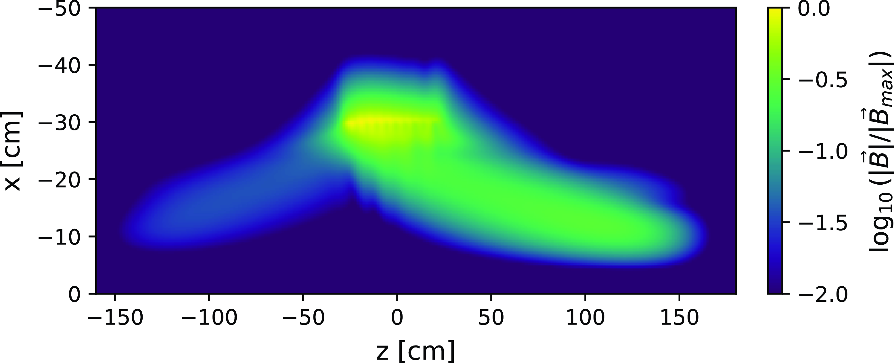
Figure 18. Comparison of directionality in wave magnetic fields from COMSOL model. Phasing in model set to launch in + $\hat {z}$
-direction.
$\hat {z}$
-direction.
Finally, we use the model to demonstrate the directional behavior of the antenna and compare with the experimental data. Figure 18 shows the model when the antenna currents are set to launch in the + $\hat {z}$
-direction. We see that the wave power is concentrated on the +
$\hat {z}$
-direction. We see that the wave power is concentrated on the + $\hat {z}$
-side of the antenna, and there is a
$\hat {z}$
-side of the antenna, and there is a $\sim 10\times$
separation in the field amplitude measured on the intended launch side compared with the opposite side of the antenna. This is similar to what was measured in the experiment.
$\sim 10\times$
separation in the field amplitude measured on the intended launch side compared with the opposite side of the antenna. This is similar to what was measured in the experiment.
7.2. RFPisa
Further comparison with modeling was conducted using the RFPisa code. This code can capture more completely the three-dimensional structure of the wave fields given the ideal antenna spectrum. Utilizing the plasma and antenna parameters from the experiment, we worked to simulate the LAPD case in RFPisa. In particular, we ensured that the quantity of modes included in the simulation was large enough to reproduce correctly the expected ideal antenna spectrum. The spatially resolved density measurements from the experiment were used to set the profile in the highest-density case, then scaled accordingly to represent the low-density cases.
7.2.1. Description of the RFPisa code
RFPisa is a one-dimensional-plasma, full-wave, hot-plasma simulation code entirely developed at TAE Technologies for the cylindrical geometry and applied to a diversity of problems (Ceccherini et al. Reference Ceccherini, Galeotti, Barnes and Dettrick2024). It is originally based on the reduced finite Larmor radius equations which include the so-called Swanson–Colestock–Kashuba approximation (Swanson Reference Swanson1981; Colestock & Kashuba Reference Colestock and Kashuba1983) and that were previously derived by M. Brambilla for toroidal geometry (Brambilla Reference Brambilla1989, Reference Brambilla1999a ,Reference Brambilla b , Reference Brambilla2012). The general vector wave equation that RFPisa solves is given by
 \begin{equation} \nabla \times \nabla \times \boldsymbol{E}(\boldsymbol{r},t) + \frac {1}{c^2} \frac {\partial ^2 \boldsymbol{E}(\boldsymbol{r},t)}{\partial t^2} = -\frac {4 \pi }{c^2} \frac {\partial }{\partial t} [ \boldsymbol{J}_{\mathrm{ant}}(\boldsymbol{r},t) + \boldsymbol{J}_{\mathrm{ pla}}(\boldsymbol{E}(\boldsymbol{r},t))], \end{equation}
where $\boldsymbol{E}({\boldsymbol{r}}, t)$
is the perturbation electric field,
$\boldsymbol{E}({\boldsymbol{r}}, t)$
is the perturbation electric field, $\boldsymbol{J}_{\mathrm{ant}}$
is the antenna current density and
$\boldsymbol{J}_{\mathrm{ant}}$
is the antenna current density and $\boldsymbol{J}_{\mathrm{pla}} (\boldsymbol{E}(\boldsymbol{r},t))$
is the plasma current density obtained from the linearized Vlasov equations. For the cylindrical geometry a substantial simplification is achieved if azimuthal symmetry and infinite length in the axial direction can be assumed. It is worth noting that these assumptions are well matched to the LAPD geometry. Once these assumptions are taken into account, a Fourier decomposition in the azimuthal and axial directions can be applied to the perturbation electric field
$\boldsymbol{J}_{\mathrm{pla}} (\boldsymbol{E}(\boldsymbol{r},t))$
is the plasma current density obtained from the linearized Vlasov equations. For the cylindrical geometry a substantial simplification is achieved if azimuthal symmetry and infinite length in the axial direction can be assumed. It is worth noting that these assumptions are well matched to the LAPD geometry. Once these assumptions are taken into account, a Fourier decomposition in the azimuthal and axial directions can be applied to the perturbation electric field
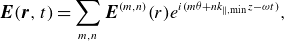 \begin{equation} \boldsymbol{E}(\boldsymbol{r},t) = \sum _{m,n} \boldsymbol{E}^{(m,n)}(r)e^{i(m\theta + n k_{\parallel , \mathrm{min}} z - \omega t ) } ,\end{equation}
where $k_{\parallel , \mathrm{ min}}$
is the lowest possible value for the parallel wavevector. The wave equation (7.5) is reduced for each mode
$k_{\parallel , \mathrm{ min}}$
is the lowest possible value for the parallel wavevector. The wave equation (7.5) is reduced for each mode $(m, n)$
to
$(m, n)$
to
 \begin{equation} \nabla \times \nabla \times \boldsymbol{E}^{(m,n)}(r)= \frac {\omega ^2}{c^2} \bigg [ \boldsymbol{E}^{(m,n)} (r)+ \frac {4\pi i}{\omega } \bigg ( \boldsymbol{J}_i^{(m,n),}(r) +\boldsymbol{J}_e^{(m,n)} (r)+\boldsymbol{J}_{\mathrm{ ant}}^{(m,n)}(r) \bigg ) \bigg ] ,\end{equation}
where $\boldsymbol{J}_i^{(m,n)}$
,
$\boldsymbol{J}_i^{(m,n)}$
, $\boldsymbol{J}_{\textrm{e}}^{(m,n)}$
and
$\boldsymbol{J}_{\textrm{e}}^{(m,n)}$
and $\boldsymbol{J}_{\mathrm{ant}}^{(m,n)}$
represent the
$\boldsymbol{J}_{\mathrm{ant}}^{(m,n)}$
represent the $(m,n)$
mode component of the electron and ion Larmor radius current (up to second order and including displacement current), and antenna current, respectively. Once the appropriate analytical expressions for the aforementioned terms are included in (7.7) the resulting equation can be reduced to a set of three coupled equations for complex electric field components. The set of coupled complex equations is discretized on a grid and solved numerically independently for each mode to obtain the corresponding electric field and hence, through Faraday’s law, the magnetic field.
$(m,n)$
mode component of the electron and ion Larmor radius current (up to second order and including displacement current), and antenna current, respectively. Once the appropriate analytical expressions for the aforementioned terms are included in (7.7) the resulting equation can be reduced to a set of three coupled equations for complex electric field components. The set of coupled complex equations is discretized on a grid and solved numerically independently for each mode to obtain the corresponding electric field and hence, through Faraday’s law, the magnetic field.
Reiterating the solution of the coupled equations through a wide range of modes allows us to generate a database which can be sourced to create Fourier three-dimensional syntheses of both electric and magnetic fields. In fact, given any antenna configuration, it is possible to compute the weight corresponding to each mode $(m, n)$
and, through an appropriate summation, to calculate the total value of any field at any location of the cylindrical volume. An example of the full three-dimensional reconstruction of the fields in the cylindrical volume is shown in figure 19. Here, the antenna modules are overlaid onto the two-dimensional plane cuts of the tangential magnetic field. In principle, any region within the simulation domain can be examined. The following section will show the resulting wave fields in the measurement region of the experiment.
$(m, n)$
and, through an appropriate summation, to calculate the total value of any field at any location of the cylindrical volume. An example of the full three-dimensional reconstruction of the fields in the cylindrical volume is shown in figure 19. Here, the antenna modules are overlaid onto the two-dimensional plane cuts of the tangential magnetic field. In principle, any region within the simulation domain can be examined. The following section will show the resulting wave fields in the measurement region of the experiment.
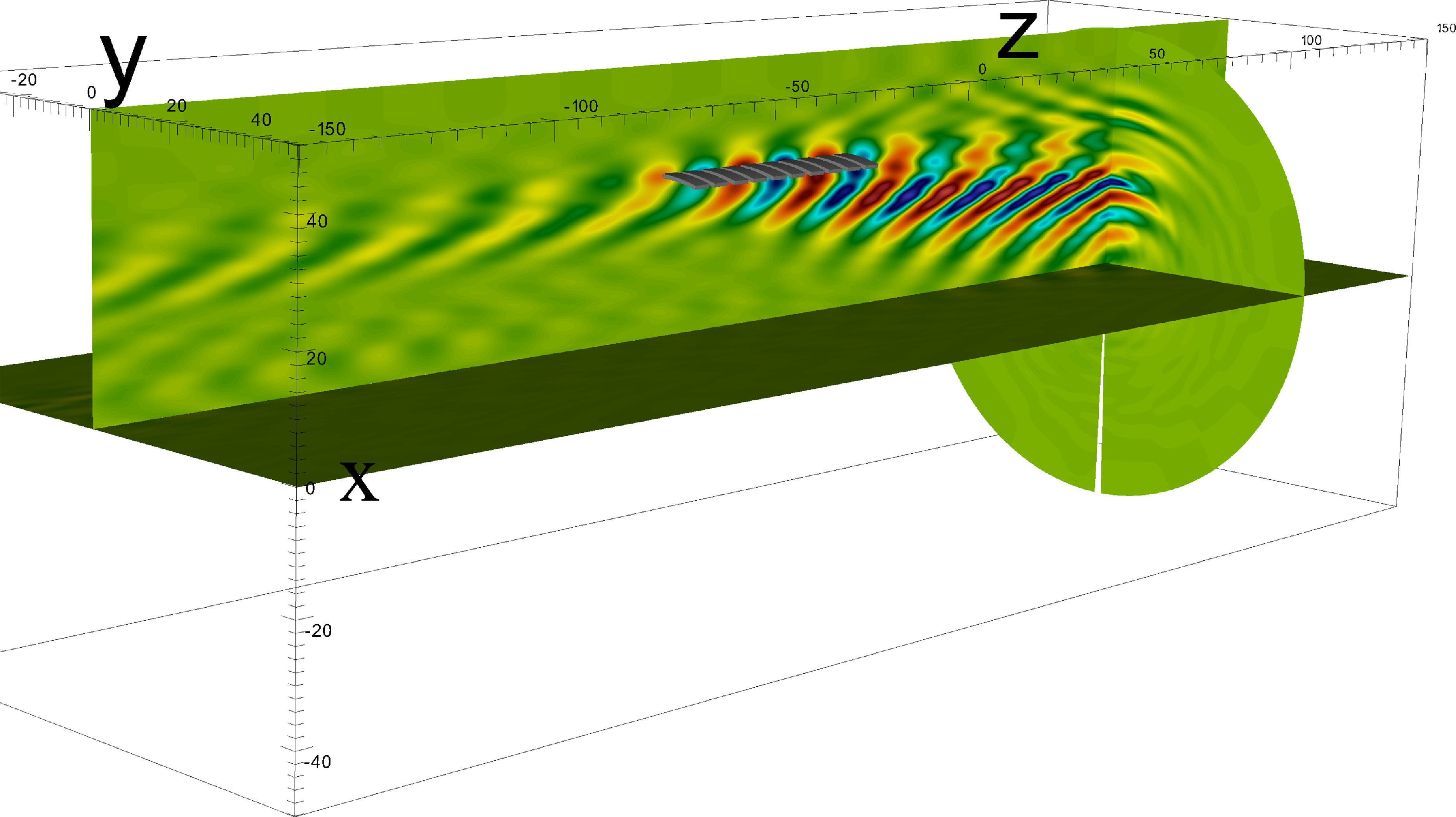
Figure 19. Two-dimensional plane cuts from three-dimensional reconstruction of experiment relevant plasma in RFPisa. Density profile used is representative of figure 6(b).
While the RFPisa code takes into account hot-plasma effects, it should be noted here that we expect little to no hot-plasma effects in the LAPD case. The low temperatures present in the LAPD make the wave dispersion well described by the cold-plasma model. The use of RFPisa here is then not to validate the code’s ability to capture the hot-plasma effects, but instead to validate the complicated multi-step process used to synthesize the full three-dimensional reconstruction of the fields. This is the first time RFPisa has been compared against experimental results, and therefore the validation shown is very important to the future applications of RFPisa.
7.2.2. Wave fields
The resulting fields calculated using the RFPisa code for the nominal $f_0=476$
MHz,
$f_0=476$
MHz, $B_0=0.2$
T case are shown in figure 20. Figure 20 shows the region of the simulation where we have taken data in the experiment. Here, we can see that, in the highest-density case (figure 20
a), when we expect that fast waves can propagate in the plasma, we do indeed see a forward-propagating mode. The intermediate density case, figure 20
b), shows the mixture of the long-wavelength fast wave as well as the short-wavelength slow mode. At the late discharge time, figure 20
c), we again see only the slow wave as the backward-propagating mode. While the wave patterns do not exactly match the experiment, we do see the same behavior of the observed waves in each of the density cases. It is not entirely surprising that there is some disagreement between the RFPisa code and the experiment. In fact, the RFPisa code is given an ideal launch spectrum from the antenna. Moreover, particularities about the antenna geometry such as the Faraday screens on the modules as well as non-ideal fields excited in front of the modules are not included. Since the exact geometry of the antenna is not included in the model, we therefore do not expect an exact match in the measured fields. The comparison here does show, however, that inclusion of a more complete description of the ideal spectrum still shows the transition of fast to slow wave launching from the antenna. From this we have seen that we can use RFPisa to confidently identify the plasma conditions necessary for an antenna that excites the ideal spectrum expected from the TWA to launch fast waves in an LAPD plasma.
$B_0=0.2$
T case are shown in figure 20. Figure 20 shows the region of the simulation where we have taken data in the experiment. Here, we can see that, in the highest-density case (figure 20
a), when we expect that fast waves can propagate in the plasma, we do indeed see a forward-propagating mode. The intermediate density case, figure 20
b), shows the mixture of the long-wavelength fast wave as well as the short-wavelength slow mode. At the late discharge time, figure 20
c), we again see only the slow wave as the backward-propagating mode. While the wave patterns do not exactly match the experiment, we do see the same behavior of the observed waves in each of the density cases. It is not entirely surprising that there is some disagreement between the RFPisa code and the experiment. In fact, the RFPisa code is given an ideal launch spectrum from the antenna. Moreover, particularities about the antenna geometry such as the Faraday screens on the modules as well as non-ideal fields excited in front of the modules are not included. Since the exact geometry of the antenna is not included in the model, we therefore do not expect an exact match in the measured fields. The comparison here does show, however, that inclusion of a more complete description of the ideal spectrum still shows the transition of fast to slow wave launching from the antenna. From this we have seen that we can use RFPisa to confidently identify the plasma conditions necessary for an antenna that excites the ideal spectrum expected from the TWA to launch fast waves in an LAPD plasma.
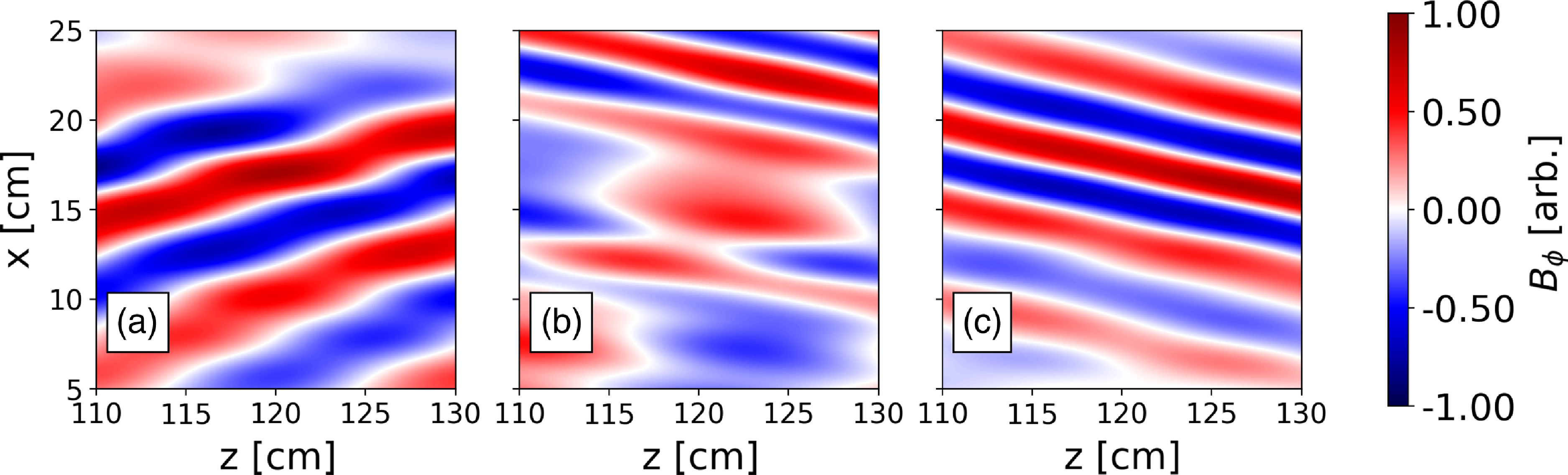
Figure 20. The RFPisa model run using 476 MHz, $B_0$
= 0.2 T case. Densities are representative of timings in corresponding panels of figure 9: (a)
$B_0$
= 0.2 T case. Densities are representative of timings in corresponding panels of figure 9: (a) $n_0=5.5\times 10^{17}$
(m
$n_0=5.5\times 10^{17}$
(m $^{-3}$
), (b)
$^{-3}$
), (b) $n_0=2.5\times 10^{17}$
(m
$n_0=2.5\times 10^{17}$
(m $^{-3}$
), (c)
$^{-3}$
), (c) $n_0=1.5\times 10^{17}$
(m
$n_0=1.5\times 10^{17}$
(m $^{-3}$
).
$^{-3}$
).
8. Summary
Throughout the work shown here we have shown that the TWA operates as designed. We have demonstrated that the TWA launches fast waves when the plasma supports fast-wave propagation. By comparing the plasma density, wave phase fronts and the cold-plasma dispersion relation, we have identified which mode was propagating in the plasma at a given time. Over a scan of antenna drive frequency, we observed changes in the measured wave fields that corresponded to the predicted changes in imposed $n_\parallel$
. The trends in the measured perpendicular wavenumber spectrum agreed well with the predicted wavenumber spectrum for the respective change in
$n_\parallel$
. The trends in the measured perpendicular wavenumber spectrum agreed well with the predicted wavenumber spectrum for the respective change in $n_\parallel$
. Using the antenna symmetry and a set of
$n_\parallel$
. Using the antenna symmetry and a set of $\dot {B}$
probes we were able to show that the antenna launches directionally, with control of the directionality determined by the choice of the feed end of the antenna structure. A survey of the loading characteristics demonstrated a change in the imposed
$\dot {B}$
probes we were able to show that the antenna launches directionally, with control of the directionality determined by the choice of the feed end of the antenna structure. A survey of the loading characteristics demonstrated a change in the imposed $n_\parallel$
with drive frequency as manifested by increased loading with the shift in the fast-wave cutoff density. The scan in static magnetic field showed that loading on the antenna was higher during times in the discharge where fast-wave propagation was observed, suggesting stronger antenna loading during fast-wave coupling. Lastly, a comparison with two models was shown. Using a cold-plasma axisymmetric model, we saw good agreement with the observed propagating modes for density profiles representative of the experiment. A clear distinction of the orientation of the phase fronts indicated fast- versus slow-wave propagation that was observed in both the model and experiment. Qualitative agreement in the directionality of the antenna was also observed. The use of the RFPisa code developed by TAE technologies showed agreement with the observation of the two plasma modes at different discharge times/densities. These two separate modeling efforts support the observations made in the experiments. As such it can be seen that the TWA design works well to launch fast waves directionally when the antenna and plasma parameters support fast-wave propagation.
$n_\parallel$
with drive frequency as manifested by increased loading with the shift in the fast-wave cutoff density. The scan in static magnetic field showed that loading on the antenna was higher during times in the discharge where fast-wave propagation was observed, suggesting stronger antenna loading during fast-wave coupling. Lastly, a comparison with two models was shown. Using a cold-plasma axisymmetric model, we saw good agreement with the observed propagating modes for density profiles representative of the experiment. A clear distinction of the orientation of the phase fronts indicated fast- versus slow-wave propagation that was observed in both the model and experiment. Qualitative agreement in the directionality of the antenna was also observed. The use of the RFPisa code developed by TAE technologies showed agreement with the observation of the two plasma modes at different discharge times/densities. These two separate modeling efforts support the observations made in the experiments. As such it can be seen that the TWA design works well to launch fast waves directionally when the antenna and plasma parameters support fast-wave propagation.
Acknowledgement
Editor Cary Forest thanks the referees for their advice in evaluating this article.
Funding
The work was performed at the Basic Plasma Science Facility, which is a DOE Office of Science, FES collaborative user facility and is funded by DOE (No. DE-FC02-07ER54918) and the National Science Foundation (No. NSF-PHY 1036140).
Declaration of interests
The authors report no conflicts of interest.


 Open access