


INTRODUCTION
Climate and environmental changes (CECs) have synergistic impacts on marine ecosystems (e.g. altering temperature, ocean circulation, nutrient concentrations and seawater pH) and can drive spatio-temporal changes in the distribution and abundance of species, with cascading effects on ecosystem functioning (Harley et al., Reference Harley, Hughes, Hultgren, Miner, Sorte, Thornber, Rodriguez, Tomanek and Williams2006; Hoegh-Guldberg & Bruno, Reference Hoegh-Guldberg and Bruno2010; Burrows et al., Reference Burrows, Schoeman, Buckley, Moore, Poloczanska, Brander, Brown, Bruno, Duarte, Halpern, Holding, Kappel, Kiessling, O'Connor, Pandolfi, Parmesan, Schwing, Sydeman and Richardson2011; Gattuso et al., Reference Gattuso, Magnan, Bille, Cheung, Howes, Joos, Allemand, Bopp, Cooley, Eakin, Hoegh-Guldberg, Kelly, Poertner, Rogers, Baxter, Laffoley, Osborn, Rankovic, Rochette, Sumaila, Treyer and Turley2015). The expected sign of CECs on marine life reaches from genetic and physiological adaptations to distributional shifts (Harley et al., Reference Harley, Hughes, Hultgren, Miner, Sorte, Thornber, Rodriguez, Tomanek and Williams2006; Poloczanska et al., Reference Poloczanska, Brown, Sydeman, Kiessling, Schoeman, Moore, Brander, Bruno, Buckley, Burrows, Duarte, Halpern, Holding, Kappel, O'Connor, Pandolfi, Parmesan, Schwing, Thompson and Richardson2013; Gotelli & Stanton-Geddes, Reference Gotelli and Stanton-Geddes2015). Under climate and environmental changes, the general prediction for marine and terrestrial species distribution, based on observations and theories, is a shift towards high latitudes, where more favourable conditions might exist, or alternatively, multi-directional distribution shifts are expected to occur (Burrows et al., Reference Burrows, Schoeman, Buckley, Moore, Poloczanska, Brander, Brown, Bruno, Duarte, Halpern, Holding, Kappel, Kiessling, O'Connor, Pandolfi, Parmesan, Schwing, Sydeman and Richardson2011; VanDerWal et al., Reference VanDerWal, Murphy, Kutt, Perkins, Bateman, Perry and Reside2013; García Molinos et al., Reference García Molinos, Halpern, Schoeman, Brown, Kiessling, Moore, Pandolfi, Poloczanska, Richardson and Burrows2015; Lenoir & Svenning, Reference Lenoir and Svenning2015). Marine organisms are valuable for assessing the possible impacts and magnitude of CECs on species distribution (Monaco & Helmuth, Reference Monaco and Helmuth2011; Riebesell & Gattuso, Reference Riebesell and Gattuso2015); one such example is ecosystem engineers, organisms that create and provide persistent habitats for the associated biodiversity (Jones et al., Reference Jones, Lawton and Shachak1997; Coleman & Williams, Reference Coleman and Williams2002). Understanding the responses of such species under CEC scenarios has become a challenge for marine ecologists. Moreover, it is crucial in forecasting possible shifts in the distributional range of ecosystem engineers under CEC (Przeslawski et al., Reference Przeslawski, Ahyong, Byrne, Wörheide and Hutchings2008).
A number of approaches (e.g. laboratory and field studies, long-term multigenerational experimental research, and modelling) have been used to assess the impacts of CECs on marine biodiversity (Wernberg et al., Reference Wernberg, Smale and Thomsen2012; Andersson et al., Reference Andersson, Kline, Edmunds, Archer, Bednarsek, Carpenter, Chadsey, Goldstein, Grottoli, Hurst, King, Kübler, Kuffner, Mackey, Menge, Paytan, Riebesell, Schnetzer, Warner and Zimmerman2015; Riebesell & Gattuso, Reference Riebesell and Gattuso2015). Numerical model simulations of species distribution generate crucial predictive models that can be useful for conservation planning (Andersson et al., Reference Andersson, Kline, Edmunds, Archer, Bednarsek, Carpenter, Chadsey, Goldstein, Grottoli, Hurst, King, Kübler, Kuffner, Mackey, Menge, Paytan, Riebesell, Schnetzer, Warner and Zimmerman2015). There is strong evidence that recent observations of sea urchin and fish distribution shifts support modelling forecasts (Poloczanska et al., Reference Poloczanska, Burrows, Brown, García Molinos, Halpern, Hoegh-Guldberg, Kappel, Moore, Richardson, Schoeman and Sydeman2016). Although there are some examples of modelling studies using multiple drivers and multiple scenarios showing shifts in marine biodiversity in the global scale (Jones & Cheung, Reference Jones and Cheung2015; García Molinos et al., Reference García Molinos, Halpern, Schoeman, Brown, Kiessling, Moore, Pandolfi, Poloczanska, Richardson and Burrows2015) or considering ecosystem engineer organisms (Couce et al., Reference Couce, Ridgwell and Hendy2013), there have been few attempts to forecast climate-driven impacts on tropical and temperate species on a large geographic scale (Saupe et al., Reference Saupe, Hendricks, Peterson and Lieberman2014). Previous modelling studies have indicated that the expected effects on the distribution of marine organisms are as follows: (i) species will exhibit poleward shifts in their distribution, (ii) tropical species will be highly vulnerable due to the contraction of suitable habitats, and (iii) the geographic distribution of suitable habitats will decrease more quickly and markedly under a scenario with high CO2 concentrations (García Molinos et al., Reference García Molinos, Halpern, Schoeman, Brown, Kiessling, Moore, Pandolfi, Poloczanska, Richardson and Burrows2015; Jones & Cheung, Reference Jones and Cheung2015). Alternatively, within groups of solely tropical or temperate species, no consistent pattern among species would occur due to varied responses in the direction of shifts or an increase/decrease in the suitable area (Saupe et al., Reference Saupe, Hendricks, Peterson and Lieberman2014). Although in recent years a large number of modelling studies have shown distributional shifts under CECs, this approach is not yet common to assess the responses in closely related ecosystem engineer species.
In temperate and tropical coastal areas around the world, some species of sabellariids build so-called worm reefs (WRs) (Zamorano et al., Reference Zamorano, Moreno and Duarte1995; Dubois et al., Reference Dubois, Retière and Olivier2002; Bremec et al., Reference Bremec, Carcedo, Piccolo, Santos and Fiori2014; Faroni-Perez, Reference Faroni-Perez2014; Firth et al., Reference Firth, Mieszkowska, Grant, Bush, Davies, Frost, Moschella, Burrows, Cunningham, Dye and Hawkins2015; Nishi et al., Reference Nishi, Matsuo, Capa, Tomioka, Kajihara, Kupriyanova and Polgar2015; Faroni-Perez et al., Reference Faroni-Perez, Helm, Burghardt, Hutchings and Capa2016), which are important biogenic structures, following hermatypic corals and stromatolites (Goldberg, Reference Goldberg2013). WRs represent habitats of high biodiversity on which hundreds of species of invertebrates and fishes rely for feeding, nursery, refuge and migration (Gherardi & Cassidy, Reference Gherardi and Cassidy1994; Dubois et al., Reference Dubois, Retière and Olivier2002; Ataide et al., Reference Ataide, Venekey, Rosa-Filho and Dos Santos2014). There is strong evidence, based on historical and recent surveys that the distribution and abundance of WRs are already changing in response to recent CECs (Firth et al., Reference Firth, Mieszkowska, Grant, Bush, Davies, Frost, Moschella, Burrows, Cunningham, Dye and Hawkins2015). In the present study, multiple drivers and scenarios were used to target future biogeographic changes in the distribution of two species of polychaetes of the Sabellariidae family that are ecosystem engineers (Coleman & Williams, Reference Coleman and Williams2002). Among the sabellariids, the genus Phragmatopoma is endemic to the American coastline, contains four valid species and is mainly registered in intertidal and shallow subtidal zones (Capa & Hutchings, Reference Capa, Hutchings, Purschke and Westheide2014; Faroni-Perez et al., Reference Faroni-Perez, Helm, Burghardt, Hutchings and Capa2016). Here, the focus was on two reef-building species, Phragmatopoma caudata, Krøyer in Mörch, Reference Mörch1863, and P. virgini, Kinberg, Reference Kinberg1866, as they are genetically close related and occur in distinctive areas (Nunes et al., Reference Nunes, Van Wormhoudt, Faroni-Perez and Fournier2016). In terms of marine biogeographic provinces (Briggs & Bowen, Reference Briggs and Bowen2012), P. caudata occurs in the tropical regions of the Western Atlantic, ranging from the Florida coast to the southern coast of Brazil, whereas P. virgini occurs in the temperate regions of the South-east Pacific Ocean ranging from Ecuador to Patagonia and northwards up to Uruguay in the South-west Atlantic Ocean.
Therefore, in order to assess if CECs will cause distribution shifts in tropical and temperate WRs, present-day habitat suitability distributions were modelled, as well as under IPCC-CMIP 5 projections for two different time intervals (mid-century: 2040–2059 and late-century: 2080–2099). The tested hypotheses was as follows: (i) under a low CO2 concentration and active atmospheric carbon capturing scenario (RCP2.6), both tropical and temperate WR species will maintain their current distributions and face only slight multi-directional biogeographic changes across the century; and (ii) under a high CO2 concentration scenario (RCP8.5), both species will shift toward high latitudes, with marked changes for tropical WRs and slight changes for temperate WRs, specifically at the end of the century.
MATERIALS AND METHODS
Datasets: species occurrences and environmental predictors
For the dataset of species occurrences, an extensive online search was performed using the keyword ‘Phragmatopoma’ in various reference databases (i.e. Web of Science, SCOPUS, SciElo, Google Scholar), the catalogue of the Smithsonian National Museum of Natural History, and the NONATOBase (Pagliosa et al., Reference Pagliosa, Doria, Misturini, Otegui, Oortman, Weis, Faroni-Perez, Alves, Camargo, Amaral, Marques and Lana2014). Additionally, original data on 57 new records was added to the dataset. Each occurrence data was georeferenced (WGS84) and record sites with low accuracy were discarded to reduce noise in the analysis. Overall, 97 literature sources were included in the analysis, resulting in 284 and 94 occurrence records for P. caudata and P. virgini, respectively.
The primary datasets of environmental drivers used are from the Coupled Model Intercomparison Project Phase 5 (IPCC, 2013; http://cmip-pcmdi.llnl.gov/cmip5/). The model selected was the HadGEM2-ES, from Met Office Hadley Centre, UK (Jones et al., Reference Jones, Hughes, Bellouin, Hardiman, Jones, Knight, Liddicoat, O'Connor, Andres, Bell, Boo, Bozzo, Butchart, Cadule, Corbin, Doutriaux-Boucher, Friedlingstein, Gornall, Gray, Halloran, Hurtt, Ingram, Lamarque, Law, Meinshausen, Osprey, Palin, Chini, Raddatz, Sanderson, Sellar, Schurer, Valdes, Wood, Woodward, Yoshioka and Zerroukat2011; Martin et al., Reference Martin, Bellouin, Collins, Culverwell, Halloran, Hardiman, Hinton, Jones, McDonald, McLaren, O'Connor, Roberts, Rodriguez, Woodward, Best, Brooks, Brown, Butchart, Dearden, Derbyshire, Dharssi, Doutriaux-Boucher, Edwards, Falloon, Gedney, Gray, Hewitt, Hobson, Huddleston, Hughes, Ineson, Ingram, James, Johns, Johnson, Jones, Jones, Joshi, Keen, Liddicoat, Lock, Maidens, Manners, Milton, Rae, Ridley, Sellar, Senior, Totterdell, Verhoef, Vidale and Wiltshire2011). The global climate model provided by HadGEM2-ES includes all components of the earth system (i.e. physical atmosphere and ocean components with the addition of schemes to characterize aspects of the Earth system) (Collins et al., Reference Collins, Bellouin, Doutriaux-Boucher, Gedney, Halloran, Hinton, Hughes, Jones, Joshi, Liddicoat, Martin, O'Connor, Rae, Senior, Sitch, Totterdell, Wiltshire and Woodward2011; Martin et al., Reference Martin, Bellouin, Collins, Culverwell, Halloran, Hardiman, Hinton, Jones, McDonald, McLaren, O'Connor, Roberts, Rodriguez, Woodward, Best, Brooks, Brown, Butchart, Dearden, Derbyshire, Dharssi, Doutriaux-Boucher, Edwards, Falloon, Gedney, Gray, Hewitt, Hobson, Huddleston, Hughes, Ineson, Ingram, James, Johns, Johnson, Jones, Jones, Joshi, Keen, Liddicoat, Lock, Maidens, Manners, Milton, Rae, Ridley, Sellar, Senior, Totterdell, Verhoef, Vidale and Wiltshire2011; Zelinka et al., Reference Zelinka, Klein, Taylor, Andrews, Webb, Gregory and Forster2013), and have been used to forecast shifts in distribution of marine and terrestrial species (Good et al., Reference Good, Jones, Lowe, Betts and Gedney2013; Saupe et al., Reference Saupe, Hendricks, Peterson and Lieberman2014; García Molinos et al., Reference García Molinos, Halpern, Schoeman, Brown, Kiessling, Moore, Pandolfi, Poloczanska, Richardson and Burrows2015; McQuillan & Rice, Reference McQuillan and Rice2015; Xavier et al., Reference Xavier, Peck, Fretwell and Turner2016). The monthly output data of the concentration of carbon, chlorophyll, dissolved nitrate, ammonium and silicate, hydrogen ion, alkalinity, air and sea surface temperature, precipitation, salinity and water runoff was acquired from HadGEM2-ES (Table 1). The dataset was divided into a ‘current’ period, which included the recent past (1986–2005), whereas future projections for the Representative Concentration Pathways (RCPs) 2.6 and 8.5 were subdivided into the ‘middle of the century’ (i.e. mid-century 2040–2059) and the ‘end of the century’ (i.e. late-century 2080–2099). These future projections represent contrasting scenarios: the RCP2.6 characterizes the optimistic and environmentally friendly future with low CO2 concentrations, and the RCP8.5 represents the worst-case scenario with the highest CO2 concentrations. Each environmental predictor was rescaled to a resolution of 0.08 × 0.08°, using bi-linear interpolation. Additionally, for each predictor, the interannual monthly mean was calculated from the primary data. The annual values (average, minimum and maximum) were then calculated totalling 36 environmental drivers layers (see online supplementary material).
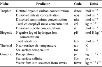
Table 1. Niches and their environmental drivers with code and units used for modelling habitat suitability.
Selection of predictors
The predictors, here classified according to the use of the source by the worms (i.e. biogenic, osmotic, thermal and trophic; see Table 1), were selected based on environmental variables representative of the key dimensions of the niche for the studied species (Austin, Reference Austin2007). This multi-dimensional niche approach was used as a step selection of variables that can influence the distribution of Phragmatopoma species. Following a hierarchical framework to reduce multi-collinearity, an array of a peer-to-peer correlation matrices using the set of layers from the ‘current’ time period was created that excluded highly correlated predictors (Pearson, r > 0.60). After this step, only nine out of initially 36 predictors remained, two for each niche dimension, except the trophic, which had three predictors per species. Subsequently, to select for each species the most representative predictor for each pre-established niche dimension, a set of generalized linear models (GLMs) was built, exploring the possible combinations of variables and considering one predictor per niche. The final sets of niche predictors per species were assessed by the most influential predictive capacity across models. The predictive capacity was ranked based on the number of times a given predictor was significant across GLM models (see online supplementary material). Final layers of predictors selected are as follows: pHmin (biogenic) and tosmin (thermal) for both the species, and frivermax (osmotic), simax (trophic) selected for P. caudata, and prmax (osmotic) and detocmax (trophic), for P. virgini. Predictors’ names and units are described in Table 1. Statistical analysis of these layers can be found in the online supplementary material.
Modelling
Maximum entropy modelling (MaxEnt) was used to model the current distributions of P. caudata and P. virgini and then project their future habitat suitability according to the future IPCC-CMIP 5 projections. MaxEnt is a correlative algorithm that uses the occurrence data of species coupled to environmental data for modelling species distributions (Phillips et al., Reference Phillips, Anderson and Schapire2006; Phillips & Dudik, Reference Phillips and Dudik2008; Elith et al., Reference Elith, Phillips, Hastie, Dudík, Chee and Yates2011) and can be used to predict the future impacts of CECs on marine organisms (Couce et al., Reference Couce, Ridgwell and Hendy2013; Verbruggen et al., Reference Verbruggen, Tyberghein, Belton, Mineur, Jueterbock, Hoarau, Gurgel and De Clerck2013; Saupe et al., Reference Saupe, Hendricks, Peterson and Lieberman2014). Generally, the models produced by MaxEnt are influenced by the extent of the study area and species occurrence, which are data input premises. Thus, the MaxEnt algorithm performs better when the study area for the calibration model does not include areas outside the species range occurrence (Anderson & Raza, Reference Anderson and Raza2010; Elith et al., Reference Elith, Phillips, Hastie, Dudík, Chee and Yates2011). For this reason, the model is calibrated with the immediately surrounding region for each species known occurrence. Subsequently, the background area of each species was referred strictly to the occurring latitudinal span and longitudinally delimited by the closest cell grid representing the continental shoreline, as the two species inhabit the intertidal or shallow subtidal zones. Additionally, the OccurrenceThinner (Verbruggen et al., Reference Verbruggen, Tyberghein, Belton, Mineur, Jueterbock, Hoarau, Gurgel and De Clerck2013) was used to filter the data and reduce the geographic sampling bias since MaxEnt better estimates the contribution of the niche environmental variables for each species, when not overestimating the model performance (Elith et al., Reference Elith, Phillips, Hastie, Dudík, Chee and Yates2011; Veloz et al., Reference Veloz, Nur, Salas, Jongsomjit, Wood, Stralberg and Ballard2013). OccurrenceThinner uses the occurrence records and a raster of a kernel density function of the study area to reduce occurrence records, omitting more records from densely sampled regions. This filtering resulted in 42 and 21 occurrence records for P. caudata and P. virgini, respectively.
For the species-specific model tuning, various potential sources of complexity from the MaxEnt features were investigated, considering methods proposed by Elith et al. (Reference Elith, Kearney and Phillips2010, Reference Elith, Phillips, Hastie, Dudík, Chee and Yates2011), Shcheglovitova & Anderson (Reference Shcheglovitova and Anderson2013) and Radosavljevic & Anderson (Reference Radosavljevic and Anderson2014) (see online supplementary material). Then, the fitted model was assessed based on the performance of explanatory predictors and MaxEnt features. The maps and results reported herein are based on the MaxEnt average (5 runs), cross-validated, logistic output, and with the clamping setting as true. The model predictions were tested by partial receiver operating characteristic analyses (p-ROC AUC) with E = 0.5 of the maximum error rate, 50% random points and 500 iterations for the bootstrap (Peterson et al., Reference Peterson, Papes and Soberon2008; Peterson, Reference Peterson2012).
Post modelling
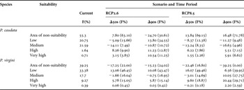
To quantify the shifts in the distribution of tropical and temperate WRs, a metric based on total grid cell values (i.e. each pixel suitability) was applied. The total numbers of grid cells were 4515 for P. caudata and 3322 for P. virgini. For each projection, grid-cell values were extracted and frequency distribution and the delta value were computed. The delta value is the relative difference in total grid-cell frequencies between each future projection and the present day. Although the threshold of minimum training presence values was 0.11 for P. caudata and 0.09 for P. virgini, the threshold value of 0.2 was set to define unsuitable areas, pixel values ≤0.2 are included in the non-suitability category (see online supplementary material). Consequently, changes in delta values correspond to a gain or a loss of suitable area. The remaining grid cells (i.e. pixel values: comprised between 0.21 and 1) correspond to the suitable area, and for which changes in the delta value were categorized as follows: 0.21 ≤ low ≤ 0.4; 0.41 ≤ medium ≤ 0.6; 0.61 ≤ high ≤ 0.8; 0.81 ≤ very high ≤ 1. This analysis attempted solely to characterize and quantify ‘potential’ shifts in the distribution of each species based on their areas of environmental suitability.
Processing all modelling
All software used in this study is listed in the online supplementary material.
Abbreviations
- CECs:
-
Climate and environmental changes.
- WRs:
-
Worm reefs built by Sabellariidae.
- RCPs:
-
Representative concentration pathways; radiative forcing values for scenario set, containing emission, concentration and land-use trajectories (van Vuuren et al., Reference van Vuuren, Edmonds, Kainuma, Riahi, Thomson, Hibbard, Hurtt, Kram, Krey, Lamarque, Masui, Meinshausen, Nakicenovic, Smith and Rose2011).
- RCP2.6:
-
Mitigation scenario leading to a very low forcing level.
- RCP8.5:
-
Very high baseline emission scenario.
RESULTS
Modelling analysis and contribution of multiple drivers
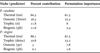
MaxEnt models showed good predictive performances for the models (Table 2). For the present-day period, the predicted areas of suitable habitat were in agreement with the current distribution of both species. The current areas of suitability cover 44.7% and 60.8% of the total extent of Phragmatopoma caudata and P. virgini, respectively. For both species, the predictors regarding the trophic and osmotic niches showed an intermediary influence in the model, although they had an inverse influential order (Table 3). The most influential predictor for both species was sea surface temperature (tos), related to the thermal niche. In contrast, pH (related to the biogenic niche) showed the lowest contribution to the model for both species (Table 3).
Table 2. Summary of model statistics showing the receiver operating characteristic curves for MaxEnt with E = 0.5 of acceptable omission error according to p-ROC AUC values.
Table 3. Influence of environmental drivers used in modelling habitat suitability. Codes used for predictors are defined in Table 1.
Future trends of habitat suitability for worm reefs
All models predicted future differences in the distribution of habitat suitability for tropical and temperate WRs (Figure 1). For the ‘optimistic scenario’ (RCP2.6), in contrast with the current distributions of both WRs, a gain of suitable areas was predicted for the end of the century. However, idiosyncratic responses were forecast; in the mid-century, tropical WRs would lose area, while temperate WRs would gain area. At the end of the century, tropical WRs would markedly increase their distribution, while temperate WRs would slightly lose area compared with the mid-century situation (Figure 1). Under the ‘business as usual’ scenario (RCP8.5), which predicts the highest temperature increase, models also showed idiosyncratic responses of tropical and temperate WRs (Figure 1). Tropical WRs tend to lose suitable areas across the century, and a majority of changes would occur up to the mid-century. In the 50s, it is expected that non-suitable areas increase by 13.84% for a total of 16.48% in the 90s (Table 4). The temperate WRs tend to gain suitable areas throughout the century and by the end of the century, all biogeographic areas would be suitable (Table 4). However, the major gain would occur up to the mid-century.
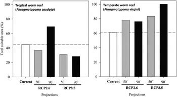
Fig. 1. Predicted changes in total suitable areas of the tropical Phragmatopoma caudata and the temperate Phragmatopoma virgini worm reefs considering current and future predictions for RCP2.6 (low emissions) and RCP8.5 (high emissions) scenarios, and the time-scales of the 50s (mid-century: 2040–2059) and the 90s (late-century: 2080–2099).
Table 4. Projected changes in the potentially suitable areas for topical (Phragmatopoma caudata) and temperate (P. virgini) worm reefs with contrast to their current habitat suitability. Δ represents the difference in frequencies of pixel suitability between current and scenarios; RCP2.6 (low emissions) and RCP8.5 (high emissions) and between the 50s (mid-century: 2040–2059) and the 90s (late-century: 2080–2099) time period. In parentheses, the total frequencies (F%) given in percentage of grid cells per projection.
BIOGEOGRAPHIC SHIFTS
Tropical worm reefs
In contrast to the current distribution, the RCP2.6 model shows opposite shifts during the century for P. caudata (Figures 1 & 2A–C). In the middle of the century, the model projected a reduction of the suitable area (~8%) in the Caribbean region, Venezuela and the northern Gulf of Mexico due to the loss of grid cells with low and medium classes of suitability. On the other hand, increments in high (~8%) and very high (~3%) classes of habitat suitability were found along the east coast of Brazil and the western part of the Gulf of Mexico (Figure 2B). Interestingly, for the end of the century, the model predicted more advantageous conditions with increasing areas and potential suitability, demonstrating the potential of species range expansion. With respect to the total area predicted as suitable, the models showed an increase from ~45% to ~69%. It is noteworthy that in the late century, 24% out of these 69% suitable areas are expected to reach the classes of high and very high suitability (Table 4). In general, areas largely in the Caribbean region, the West Indies, the western coast of the Gulf of Mexico and the coast of Brazil are herein projected as suitable (Figure 2C), with only small gaps of non-suitable areas in northern South America and the northern part of the Gulf of Mexico.
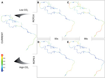
Fig. 2. Maps* show spatial variation in current (A) and future (B–E) potential suitable area distributions for tropical worm reefs (Phragmatopoma caudata) predicted given the RCP2.6 (low-emission) and RCP8.5 (high-emission) scenarios. Each projection (i.e. current, 50s and 90s) is based on a dataset covering two decades. Pixel colours correspond to the following: 0–0.2 = area of non-suitability (cold colours: medium to dark blue), 0.4 ≤ low ≤ 0.2 1(colours: light blue to green); 0.41 ≤ medium ≤ 0.4 (colours: green to light green); 0.61 ≤ high ≤ 0.8 (colours: light green to yellow); 0.81 ≤ very high ≤ 1 (warm colours: orange to red). *Continental shoreline of the tropical regions of the Western Atlantic, ranging from Florida coast (USA) to the southern coast of Brazil.
Under the RCP8.5 model, a considerable contraction was observed of the total area of potential distribution from the current (~45%) to the middle (~31%) and the end of the century (~28%; Figure 2A, D, E; Table 4). In general, an increase of non-suitable areas is projected for the entire northern part of South America, the Caribbean region, the West Indies, and the south-western and northern parts of the Gulf of Mexico. Furthermore, of the total remaining suitable area, a significant amount is classified into the low and medium classes of suitability (mid-century: ~21%, late-century: ~14%; Table 4), demonstrating vulnerability due to a massive loss of suitability. Finally, the remaining suitable areas with high and very high classes of suitability (mid-century: ~10%, late-century: ~14%) are projected for the north-western region of the Gulf of Mexico and the south-eastern part of Brazil (Figure 2D, E).
Temperate worm reefs
Under the RCP2.6 modelling outputs, Phragmatopoma virgini showed a gradual trend of a spreading distribution with increasing values of the potential suitability of habitat over the century (Figure 3A–C; Table 4). It is noteworthy that in contrast to present-day conditions, the suitability increases by 17.25% by the mid-century, reaching 78% of potential habitat suitability over the biogeographic province. Overall, projected areas that gain suitability are found towards the north of Peru and South Patagonia (Argentina and Chile), demonstrating multi-directional distribution shifts. In contrast to the mid-century, a slight increment (~2%) of the area of suitability for the end of the century was found. Furthermore, increasing values in the potential suitability for the low (~13–10%) and high (~5%) classes was observed throughout the century, regardless of a slight loss (1.6–0.75%) of the medium, indicating that P. virgini might retain its distributional range under this optimistic scenario. The biogeographic areas with increases in potential suitability were Ecuador, along the Peru coastline, and in Chile, mainly for the central part at Regions III–VII (i.e. Atacama, Coquimbo, Valparaíso, O'Higgins and Maule).
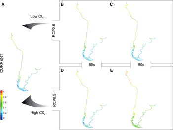
Fig. 3. Maps* show spatial variation in current (A) and future (B–E) potential suitable area distributions for temperate worm reefs (Phragmatopoma virgini) predicted given the RCP2.6 (low emissions) and RCP8.5 (high emissions) scenarios. Each projection (i.e. current, 50s and 90s) is based on a dataset covering two decades. Pixel colours correspond to the following: 0–0.2 = area of non-suitability (cold colours: medium to dark blue), 0.4 ≤ low ≤ 0.2 1(colours: light blue to green); 0.41 ≤ medium ≤ 0.4 (colours: green to light green); 0.61 ≤ high ≤ 0.8 (colours: light green to yellow); 0.81 ≤ very high ≤ 1 (warm colours: orange to red). *Continental shoreline of the temperate regions ranging from Ecuador in South-east Pacific Ocean and Uruguay in South-west Atlantic Ocean southward to Patagonia.
Under the RCP8.5 model, a gain of suitable areas during the century was also predicted (Figure 3A, D, E; Table 4). The projections show that by mid-century, 83.2% of the biogeographic province will be suitable for P. virgini. In this period, increases in the classes of low (~16%) and high (~10%) suitability were projected, notably demonstrating species gain in suitable distribution. The potential suitability is expected to increase along the coast of Ecuador, Peru and Chile (i.e. north and central coast) in the Pacific Ocean and in Uruguay and Argentina (i.e. Buenos Aires towards south of Chubut) in the Atlantic Ocean. In general, only small gaps of remaining non-suitable area in Southern Chile (i.e. Regions XI Aisén and XII Magallanes and Antártica Chilena) and Argentina (i.e. Tierra del Fuego and Santa Cruz) were observed. Finally, regarding the projection for the end of century, no grid cell is projected to be a non-suitable area, indicating that all of the P. virgini biogeographic provinces will be potentially suitable. Coupled to this evident gain of suitable area, the increments were projected into the medium (~10%) and high (~20%) classes of suitability.
DISCUSSION
Biogeographic shifts of temperate and tropical worm reefs are idiosyncratic to the climate and environmental change scenarios considered. Overall, models showed an increase in suitable habitats for temperate WRs, with a varying magnitude depending on scenarios and time periods. For the tropical WRs, responses were generally more antagonistic, also depending on the scenario and period considered. This study was the first attempt at modelling the future distribution of polychaetes using multiple drivers under IPCC-CMIP 5 scenarios. Even though the values from different modelling approaches should not be comparable (Guillera-Arroita et al., Reference Guillera-Arroita, Lahoz-Monfort, Elith, Gordon, Kujala, Lentini, McCarthy, Tingley and Wintle2015), projections from a previous study using multiple drivers under IPCC-CMIP 5 scenarios have also shown that among marine invertebrates, idiosyncratic responses to CECs are expected to occur (Saupe et al., Reference Saupe, Hendricks, Peterson and Lieberman2014).
The assumptions for temperate and tropical WRs under RCP2.6 and RCP8.5 scenarios did apply only in part. To clarify, under RCP2.6, multi-directional changes in habitat suitability would occur, but projections showed that at the end of the century, the magnitude of changes is either slight or marked for the temperate and tropical WRs, respectively. Additionally, in the case of scenario RCP8.5, marked changes in the distribution pattern were observed across the century for both species, but a consistent southward shift with suitable retraction at low latitudes was found for tropical WRs only, whereas temperate WRs exhibited continuous multi-directional shifts. Therefore, the present results suggest that the common assumptions of higher latitude range shifts cannot be globalized, as the level of CEC conditions (i.e. the different scenarios and regional impacts) and species tipping points (i.e. tropical, temperate or pandemic) also need to be considered.
Environmental variables and insights into scales
In the present models, drivers’ contribution rates differed between congeners, corroborating previous studies, which showed that CECs would not equally impact distinct biogeographic regions (Brierley & Kingsford, Reference Brierley and Kingsford2009), and that temperate and tropical species would have different responses. Tropical species are expected to be more vulnerable than temperate ones (Rosa et al., Reference Rosa, Lopes, Pimentel, Faleiro, Baptista, Trübenbach, Narciso, Dionísio, Pegado, Repolho, Calado and Diniz2014). Although demonstrating different patterns for either reef builder, sea surface temperature was the most important predictor, whereas pH played a minor role in explaining the distribution of suitable areas. This result is congruent with previous modelling studies conducted for bio-engineering corals (Couce et al., Reference Couce, Ridgwell and Hendy2013). However, it is possible that the model could have underestimated the role of pH for WRs habitat suitability. In the absence of actions to reduce CO2 emissions, within the next few decades, seawater pH values will represent a negative impact for marine invertebrates (Orr et al., Reference Orr, Fabry, Aumont, Bopp, Doney, Feely, Gnanadesikan, Gruber, Ishida, Joos, Key, Lindsay, Maier-Reimer, Matear, Monfray, Mouchet, Najjar, Plattner, Rodgers, Sabine, Sarmiento, Schlitzer, Slater, Totterdell, Weirig, Yamanaka and Yool2005; Shirayama & Thornton, Reference Shirayama and Thornton2005). Furthermore, the underwater solidification of cement used by sabellariids to build their tubes, and, consequently, the reefs, appears to be initially dependent on pH differences between the worms’ secretory glands and seawater (Stevens et al., Reference Stevens, Steren, Hlady and Stewart2007; Wang & Stewart, Reference Wang and Stewart2012). Further experiments are required to better assess the vulnerability of WRs to pH under future ocean acidification scenarios and shed light on the accuracy of models to predict the impact of low pH on shifts of species distribution. The projected increase of CO2 into the atmosphere and subsequent environmental changes throughout this century will enhance either risk: the vulnerability of tropical WRs at low latitudes and the spread of temperate WRs at high latitudes, both of which will have cascading effects on ecosystem functioning. Although warming seawater by itself would not be the unique driver to constraining biodiversity (Gattuso et al., Reference Gattuso, Magnan, Bille, Cheung, Howes, Joos, Allemand, Bopp, Cooley, Eakin, Hoegh-Guldberg, Kelly, Poertner, Rogers, Baxter, Laffoley, Osborn, Rankovic, Rochette, Sumaila, Treyer and Turley2015), the thermal predictor had the highest contribution to models.
Species distribution models and the method herein used consider that occupied grid cells estimate suitable environmental conditions, and the set of abiotic traits in these occupied cells is more favourable than adjacent unoccupied cells and non-similar abiotic traits. The geographic scale dealt with in this study encompasses a large part of the American continent. Both worm species modelled have a wide-range distribution at the continental scale, indicating that differences in local and micro-habitat variables have a relatively low importance in understanding and predicting species distribution at larger spatial scales. Spatially, the predictor layers used in this study provide sensible results at continental scales that are not necessarily accurate to local scale. Care should be applied to considerations about suitable pixel and grid cell size due to some peculiarities at fine scale, which might not be favourable for these species considering biotic (e.g. tipping points and intrinsic settlement ability) and abiotic factors (e.g. substratum availability). For example, in a grid cell a river runoff can drop coastal marine salinity to unfavourable values. In fact several WRs occur in coastal areas adjacent to estuaries (see in Faroni-Perez, Reference Faroni-Perez2014; Aviz et al., Reference Aviz, Pinto, Ferreira, Rocha and Rosa-Filho2017; Eeo et al., Reference Eeo, Chong and Sasekumar2017). During low tides WRs can cope with rain. Therefore, WRs often undergo salinity fluctuation (i.e. euryhaline to mesohaline), but no empirical data indicate that continually low salinity values (i.e. mesohaline to oligohaline) are favourable. The species modelled have wide-range distributions, however, at local spatial scales WRs do not have a homogeneous distribution. For example, low recruitment ratios in P. caudata were associated with the passage of cold fronts that dispersed larvae along coastline (Faroni-Perez, Reference Faroni-Perez2014). Although larvae can drift to different locations, they have preferences to settle gregariously onto specific substrata, a behaviour associated with sensory organs (Faroni-Perez et al., Reference Faroni-Perez, Helm, Burghardt, Hutchings and Capa2016). Larvae settle preferentially on existing reef or hard substrata, and substratum trait (type, density, over area, heterogeneity) might exert significant influence on the models. However, marine species distribution modelling lacks high resolution intertidal geological layers encompassing the American continents and hence this predictor was not considered in the present study. In some places around the world sabellariid reefs can be found directly on soft bottoms (Faroni-Perez et al., Reference Faroni-Perez, Helm, Burghardt, Hutchings and Capa2016), but that is not common among species of the genus Phragmatopoma.
Present results indicated that distribution shifts in WRs would occur. Studies have demonstrated that cost-effective methodological approaches, such as scaling up (Ferrari et al., Reference Ferrari, McKinnon, He, Smith, Corke, González-Rivero, Mumby and Upcroft2016; González-Rivero et al., Reference González-Rivero, Beijbom, Rodriguez-Ramirez, Holtrop, González-Marrero, Ganase, Roelfsema, Phinn and Hoegh-Guldberg2016), can be applied to target regional areas (e.g. 10–10,000 km) toward acquiring empirical data on distribution shifts. Further studies are encouraged to use the scaling up approaches for monitoring WRs and their associated biodiversity by a well-established temporal assessment as a key measure to detect distribution shifts as response to short-term CEC events, such as heatwaves or cold spells. Global impacts of CECs on marine biodiversity are inevitable (Harley et al., Reference Harley, Hughes, Hultgren, Miner, Sorte, Thornber, Rodriguez, Tomanek and Williams2006; Poloczanska et al., Reference Poloczanska, Hoegh-Guldberg, Cheung, Pörtner, Burrows, Field, Barros, Dokken, Mach, Mastrandrea, Bilir, Chatterjee, Ebi, Estrada, Genova, Girma, Kissel, Levy, Maccracken, Mastrandrea and White2014; Gattuso et al., Reference Gattuso, Magnan, Bille, Cheung, Howes, Joos, Allemand, Bopp, Cooley, Eakin, Hoegh-Guldberg, Kelly, Poertner, Rogers, Baxter, Laffoley, Osborn, Rankovic, Rochette, Sumaila, Treyer and Turley2015), and identifying them as a matter of urgency would promote better strategies for management actions attempting to reduce the adverse effects for biodiversity conservation.
Tropical and temperate worm reefs under the RCP2.6
Under the optimistic scenario, projections of suitable areas will persist for congeners at the end of the century, indicating the benefits for WRs to guarantee range maintenance. Similar results of suitable area persistence were found for the gastropods Bulla occidentalis and Conus spurius (see online Table S2.1, MaxEnt, all variables in Saupe et al., Reference Saupe, Hendricks, Peterson and Lieberman2014), and interestingly, the range of these molluscs co-occurs with tropical P. caudata. Across the century, temperate reefs will continually gain suitable areas, whereas tropical reefs will face an initial reduction up to the middle of the century followed by recovery and the gain of newly suitable areas at the end of the century. A decrease in habitat suitability up to the middle of the century followed by a recovery in suitability were also found for several tropical and temperate molluscs, such as Anomia simplex, Dinocardium robustum, Lucina pensylvanica, Conus spurius, Crepidula fornicata, Melongena corona, Oliva sayana, Strombus alatus and Terebra dislocata (see online Table S2.1, MaxEnt, all variables, 2041–2060 and 2081–2100 in Saupe et al., Reference Saupe, Hendricks, Peterson and Lieberman2014). These projections appear very likely when taking into account that the RCP2.6 scenario anticipates that increasing greenhouse gas emissions will peak in the middle of the century, with a subsequent drop to zero due to low emissions and the active removal of atmospheric greenhouse gases (IPCC, 2013). Then, under this peak-and-decline scenario, biodiversity will face alterations in the environment, which are expected to result in mild changes. Moreover, the present results are also consistent with a previous study, which showed that shifts by the middle of the century (2040–2059) will be much slower under the RCP2.6 scenario compared with the RCP8.5 scenario (Jones & Cheung, Reference Jones and Cheung2015). This highlights the importance of promoting effective actions on carbon emission reduction and minimizing the impacts on biodiversity.
Multi-directional shifts will be expected at the end of the century for both temperate and tropical WRs, and potential cascading effects are not likely to occur. Therefore, the majority of the new area will have a low class of potential habitat suitability. For instance, for tropical WRs, most of the projected gain in suitability will occur in the Caribbean region, but it is not evident that WRs will spread toward that area. Firstly, these areas are hotspots of biodiversity well known for their tropical coral reefs and fish communities (Floeter et al., Reference Floeter, Rocha, Robertson, Joyeux, Smith-Vaniz, Wirtz, Edwards, Barreiros, Ferreira, Gasparini, Brito, Falcón, Bowen and Bernardi2008), and sessile organisms undergo high rates of space competition (Lopez-Victoria et al., Reference Lopez-Victoria, Zea and Wei2006). Secondly, as experiments have demonstrated that polyps can survive under this optimistic scenario (Fine & Tchernov, Reference Fine and Tchernov2007), coral reefs may not face high mortality, and space competition rates would remain high, minimizing chances for the larval settlement of sabellariids. Thirdly, in the Caribbean region, many constraints prevent the establishment of WRs, a reason why they commonly do not occur where coral reefs exist (Goldberg, Reference Goldberg2013). Overall, under this environmentally friendly scenario, results indicate some crucial perspective: temperate and tropical WRs will not have their existence threatened, which benefits the associated fauna as well. There is not much evidence of negative cascading effects for the established community.
Tropical and temperate worm reefs under RCP8.5
Under the business-as-usual scenario, projections of suitable areas will markedly decrease for tropical WRs and increase for temperate WRs, either case indicating crucial issues for ecosystem functioning. The singular pattern of changes between congeners can be related to species-specific responses under future variability in the conditions of multiple drivers (Poloczanska et al., Reference Poloczanska, Brown, Sydeman, Kiessling, Schoeman, Moore, Brander, Bruno, Buckley, Burrows, Duarte, Halpern, Holding, Kappel, O'Connor, Pandolfi, Parmesan, Schwing, Thompson and Richardson2013). Some marine species can have plastic responses, such as thermal acclimation (Somero, Reference Somero2002; Helmuth et al., Reference Helmuth, Broitman, Blanchette, Gilman, Halpin, Harley, O'Donnell, Hofmann, Menge and Strickland2006), a phenomenon particularly common in invertebrates with planktonic dispersal (Sanford & Kelly, Reference Sanford and Kelly2011). Temperate (i.e. cold-water adapted) species are supposed to be more tolerant to global warming compared with their tropical (i.e. warm-water adapted) counterparts, mainly because the latter live close to their thermal tolerance limits (Tewksbury et al., Reference Tewksbury, Huey and Deutsch2008; Somero, Reference Somero2010; Nguyen et al., Reference Nguyen, Morley, Lai, Clark, Tan, Bates and Peck2011). This could support the habitat persistence and amplification of temperate WRs and the range contraction at the tropics found for tropical WRs. The response found for temperate WRs, however, is not uni-directional and may promote spatial homogenization, since habitat suitability amplifies across the whole biogeographic province. CECs promote a trend towards spatial homogenization of marine communities due to species distributional shifts or even decreases in survivorship rates (Garrabou et al., Reference Garrabou, Coma, Bensoussan, Bally, Chevaldonne, Cigliano, Diaz, Harmelin, Gambi, Kersting, Ledoux, Lejeusne, Linares, Marschal, Perez, Ribes, Romano, Serrano, Teixido, Torrents, Zabala, Zuberer and Cerrano2009; García Molinos et al., Reference García Molinos, Halpern, Schoeman, Brown, Kiessling, Moore, Pandolfi, Poloczanska, Richardson and Burrows2015). For instance, several marine organisms were affected by mass mortality events or have retracted their distribution ranges, whereas others have extended their distribution, mostly followed by recent climatic anomalies, such as heatwaves and winter storms (Garrabou et al., Reference Garrabou, Coma, Bensoussan, Bally, Chevaldonne, Cigliano, Diaz, Harmelin, Gambi, Kersting, Ledoux, Lejeusne, Linares, Marschal, Perez, Ribes, Romano, Serrano, Teixido, Torrents, Zabala, Zuberer and Cerrano2009; Wernberg et al., Reference Wernberg, Smale and Thomsen2012; Firth et al., Reference Firth, Mieszkowska, Grant, Bush, Davies, Frost, Moschella, Burrows, Cunningham, Dye and Hawkins2015).
At the end of the century, the majority of areas at low latitudes will become unsuitable for tropical WRs, most likely due to CEC-mediated shifts of distribution towards higher latitudes. This result matches predictions that the impacts of CECs would be severe in the tropics (Tewksbury et al., Reference Tewksbury, Huey and Deutsch2008; Poloczanska et al., Reference Poloczanska, Brown, Sydeman, Kiessling, Schoeman, Moore, Brander, Bruno, Buckley, Burrows, Duarte, Halpern, Holding, Kappel, O'Connor, Pandolfi, Parmesan, Schwing, Thompson and Richardson2013). Poleward expansion and equatorial contraction in distribution were also found by modelling coral reefs (Couce et al., Reference Couce, Ridgwell and Hendy2013). Currently, CECs are already causing distribution shifts towards higher latitudes in several tropical marine species, from phytoplankton to fishes (Wernberg et al., Reference Wernberg, Russell, Moore, Ling, Smale, Campbell, Coleman, Steinberg, Kendrick and Connell2011; Poloczanska et al., Reference Poloczanska, Hoegh-Guldberg, Cheung, Pörtner, Burrows, Field, Barros, Dokken, Mach, Mastrandrea, Bilir, Chatterjee, Ebi, Estrada, Genova, Girma, Kissel, Levy, Maccracken, Mastrandrea and White2014). The loss of suitability in the tropical Western Atlantic Ocean predicted for tropical WRs will probably mediate cascade effects on local communities. Consequent to a WR range contraction at low latitudes, associated species are also expected to decline due to a loss of habitat. Generally, present results corroborate several modelling forecasts for the distribution of fishes, bio-engineering corals and other invertebrates, demonstrating a marked decline in habitat suitability in tropical regions that would promote local extinction (Cheung et al., Reference Cheung, Lam, Sarmiento, Kearney, Watson and Pauly2009; Couce et al., Reference Couce, Ridgwell and Hendy2013). Then, since hotspots of biodiversity are mainly located in tropical and subtropical areas (Brown, Reference Brown2014), model predictions indicate grave ecological issues for ecosystem functioning, and marine biodiversity at low latitudes will be threatened.
The projected range extension of temperate WRs would incorporate ecological issues for local communities. For example, heat-tolerant species can display plastic responses to CECs or may even be able to shift their ranges over time for new latitudes tracking thermal niches (Somero, Reference Somero2002). Within the genus Phragmatopoma, life-history traits indicate they are r-strategists. For instance, WRs can have an average of 65,000 individuals m−2 (Faroni-Perez, Reference Faroni-Perez2014) with each female able to spawn 1500–2000 oocytes (McCarthy et al., Reference McCarthy, Young and Emson2003), and the dispersal and substrate colonization rates by juveniles are high (Zamorano et al., Reference Zamorano, Moreno and Duarte1995; Faroni-Perez, Reference Faroni-Perez2014). Moreover, WRs can dominate the substratum and exclude less competitive species (Taylor & Littler, Reference Taylor and Littler1982). Therefore, it is likely that P. virgini will have the ability to persist and colonize new suitable sites along the South-American coasts, which would promote negative cascading effects. Since WRs provide ecosystem services for many organisms, it is very likely that the associated species may also extend their ranges by tracking the existence of reefs. Thus, the multi-directional persistence of temperate WRs might facilitate the dispersion and biological invasions of the associated fauna into new territories. Some potential biological invasions in marine ecosystems promoted by CECs have already been reported, for example to solitary and colonial ascidians and encrusting bryozoans (Stachowicz et al., Reference Stachowicz, Terwin, Whitlatch and Osman2002), and it is suggested that they will be more intense at high latitudes (Cheung et al., Reference Cheung, Lam, Sarmiento, Kearney, Watson and Pauly2009; de Rivera et al., Reference de Rivera, Steves, Fofonoff, Hines and Ruiz2011). Another plausible issue is that if dense aggregations of WRs can exert physical pressure resulting in space competition (Taylor & Littler, Reference Taylor and Littler1982), then the population dynamics of pre-established adjacent organisms such as algae, anemones and molluscs will face disturbances. Thus, the enlargement of habitat suitability found for temperate WRs may drive key changes in community composition and productivity by outcompeting sensitive species.
In the Atlantic Ocean, WRs formed by the tropically distributed P. caudata are flanked in the south by Sabellaria nanella followed by P. virgini. End of century projections forecast a southward increase in habitat suitability for P. caudata and a northward increase in habitat suitability for P. virgini, making all three taxa potentially overlap their distributions around latitudes 25° and 40°S. The future trend towards sympatry among these three western Atlantic sabellariids represents an interesting ecological scenario. There is a potential for reef forming organisms to coexist through spatial and temporal niche partitioning (Knowlton & Jackson, Reference Knowlton and Jackson1994). Sympatry can drive novel patterns of resource utilization and habitat occupation. Some sympatric gregarious sabellariid species are known to exist in the same reef habitats, e.g. Neosabellaria cementarium and Idanthyrsus ornamentatus (Posey et al., Reference Posey, Marshall and Graham1984; Pawlik & Chia, Reference Pawlik and Chia1991), but mostly WRs are biogenic structures of a single species. Among WRs, spatial niche tuning can be mediated by pelagic-benthic processes through the larvae sensory organs and the intrinsic ability to select specific reef microhabitats to settle (Pawlik & Chia, Reference Pawlik and Chia1991; Faroni-Perez et al., Reference Faroni-Perez, Helm, Burghardt, Hutchings and Capa2016). Moreover, zonation preferences can lead to local niche partitioning. For example, the majority of S. nanella records come from subtidal areas, although recently some records have been noted in the intertidal (Bremec et al., Reference Bremec, Carcedo, Piccolo, Santos and Fiori2014), while the majority of P. caudata and P. virgini records are from the intertidal. Niche overlap between species has been described to WRs such as between N. cementarium and I. ornamentatus (Posey et al., Reference Posey, Marshall and Graham1984) and Sabellaria alveolata and S. spinulosa (Holt et al., Reference Holt, Hartnoll and Hawkins1997). Temporal niche partitioning can also occur through physiological and reproductive strategies. For example, biological rhythms of gametogenesis, spawning and recruitment can be different in phylogenetically closely related sabellariids (see in Eckelbarger, Reference Eckelbarger1979; McCarthy et al., Reference McCarthy, Young and Emson2003; Culloty et al., Reference Culloty, Favier, Ni Riada, Ramsay and O'Riordan2010; Faroni-Perez, Reference Faroni-Perez2014; Faroni-Perez & Zara, Reference Faroni-Perez and Zara2014; Aviz et al., Reference Aviz, Pinto, Ferreira, Rocha and Rosa-Filho2017). Another possible outcome of the potential future distributional overlap is the formation of a hybrid zone. In the laboratory, some sabellariids are able to interbreed, for example Phragmatopoma caudata, P. californica, Idanthyrsus ornamentatus and Neosabellaria cementarium (Smith & Chia, Reference Smith and Chia1985; Pawlik & Chia, Reference Pawlik and Chia1991), however developed larvae are abnormal. To date there is no evidence that P. caudata, P. virgini and S. nanella have similar spawning periods and would interbreed in situ. Synchronous spawning, interbreeding and hybrid larvae deficiency would reduce fecundity, leading to local WRs decline of one or more species. These results encourage further studies to investigate whether a more finely tuned niche partitioning can support sympatric WR species under future CEC scenarios.
Overall, the present results highlight that the distribution of two important ecosystem-engineers species will shift, and depending on the future CEC scenarios, the species will have idiosyncratic, poleward or multi-directional responses. Although under the more optimistic scenario (RCP2.6), model predictions indicate the minimization of biodiversity loss and abrupt community changes, the predictions for the worst-case RCP scenario (RCP8.5) indicate range retraction/expansion and shifts for the distribution of worm reefs. Finally, it should be considered that in order to make more exact model predictions about the magnitude of multiple-drivers (e.g. salinity, nutrients and pH) on future species distribution, experimental approaches are needed to resolve potential physiological thresholds and authenticate the modelling calibration.
SUPPLEMENTARY MATERIAL
The supplementary material for this article can be found at https://doi.org/10.1017/S002531541700087X.
ACKNOWLEDGEMENTS
The author would like to thank C.F.D. Gurgel, N. Schubert, P. Pagliosa and S. Floeter for their thoughtful comments on an earlier version of the manuscript. P. Riul was very helpful with sampling bias analysis and environmental predictors. The author is grateful to the anonymous reviewers and the Editor, Dr A. Holmes, for their constructive comments, which contributed to improving the quality of this paper. The author also acknowledges the Centre for Environmental Data Analysis (CEDA), on behalf of British Atmospheric Data Centre (BADC) and Natural Environment Research Council's (NERC) for access to the CMIP5 multi-model dataset.
FINANCIAL SUPPORT
The author was supported by the National Council for Scientific and Technological Development of Brazil (CNPq – SWE 201233/2015-0) and Coordenação de Aperfeiçoamento de Pessoal de Nivel Superior (CAPES). This paper is part of her PhD thesis.


