


I. Introduction
Saignée, the practice of bleeding juice from a batch of wine, is a widely used technique for concentrating flavor in red wine. Bleeding off a small fraction of juice in this manner reduces the quantity of red wine produced, but increases the skin-to-juice ratio, thus concentrating its phenols. Typical saignée amounts range from 10 to 20% of the total volume of juice (Godden, Reference Godden2019). However, this juice is not wasted; it is typically repurposed as rosé wine or blended with primary wine to achieve certain flavor profiles.Footnote 1 While every winemaker has her own secret formula for how much saignée to bleed off, we argue that this is fundamentally an economic question that must balance the quantity and quality of the primary wine and rosé.
The practice of saignée is nowadays well-known and common in many winemaking regions, although our review of the literature did not uncover a clear reference to its origin. A relatively small literature studies the oenological benefits of saignée, where researchers experimentally vary the volume of juice removed and report the phenolic characteristics associated with the various saignée treatments.Footnote 2 The evidence from this literature is mixed, with some studies documenting positive impacts and others reporting null impacts (e.g., Singleton, Reference Singleton1972; Gerbaux, Reference Gerbaux1993). Since there is no universally-accepted approach to saignée, different studies apply different fractions to different grapes, further complicating comparison of results across studies.Footnote 3 Based on this literature, it is tempting to think that a winemaker's objective is to choose a saignée fraction that maximizes the quality of the resulting primary wine. In this paper, we argue that while this is certainly an important margin to consider, it fails to recognize fundamental tradeoffs along other margins. Indeed, we will show that only in corner or knife-edge cases is it in the economic best interest of the winemaker to choose how much to saignée in this intuitive manner.
While the oenological literature analyzes the phenolic and wine quality benefits of saignée, it provides few insights on its economic implications. Naturally, saignée applied at any level over the original volume of juice will result in a loss of final primary wine.Footnote 4 Such loss can be potentially offset by marketing the resulting rosé wine and by selling the higher-quality primary wine for a higher price than could have been achieved in the absence of saignée. Therefore, we argue that the winemaker's choice of a saignée fraction is fundamentally an economic matter that must balance the quantity, quality, and price of the primary wine resulting from a choice of a saignée fraction and the value of the rosé wine produced as a byproduct. It is in this sense that we argue that the effect of saignée on the quality of the primary wine—the focus of the oenological literature—is only one of several margins to be considered.
In this paper, we develop what we believe is the first economic model of saignée in winemaking. We use the model to illuminate the full set of tradeoffs, and derive a set of theoretical propositions that provide both practical guidance about economically optimal saignée fractions, and empirically testable predictions about what we should observe in the wine market. Using the model, we derive the conditions under which it is optimal for a winemaker to engage in zero saignée (and thus produce only primary wine), complete saignée (and thus produce only rosé), or an intermediate amount of saignée. A key finding is that, except in corner and knife-edge cases, the profit-maximizing saignée fraction is less than the quality-maximizing fraction. Although we leave detailed empirical analysis for future work, in the final section we discuss how our results accord with observed saignée practices.
II. The model
Consider the problem facing a single winemaker trying to maximize profit from her choice of saignée. Let Q be the total quantity of juice available to the winemaker (assumed to be exogenous), which will be divided into a saignée fraction S, and a primary wine fraction (1 − S). This ultimately produces Q r = QS quantity of rosé and Q p = Q(1 − S) primary wine.Footnote 5 While the saignée fraction S will surely affect the quality of the primary wine, and indeed, this is often the winemaker's primary concern, it has no consequence for the quality of the rosé. To capture this, we assume that the price of rosé (P r) is exogenously given and independent of S, and that the price of the primary wine depends on the saignée fraction S: P p = f(S), where f(S) has a maximum at  $\bar{S}$.Footnote 6 We assume each winemaker knows $\bar{S}\in [ 0, \;1] $ for its grape profile.Footnote 7
Suppose that the cost of turning Q liters of juice into wine is cQ, which is independent of the saignée fraction S. All of this implies the following expression for profits:
 $$\pi ( S) = P_rQ_r + f( S) ( Q-Q_r) - cQ$$
 $${\hskip 2.6pc= {P_rQS} + {f( S) ( Q} - {QS) \ } - {\ cQ}}$$
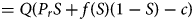 $${\hskip 1.3pc= Q( {P_rS + f( S) ( 1-S) -c} ) }$$
Since profit is linear in Q, we normalize it out, and since c plays no role in the first-order conditions, we will omit it. This yields the following simplified profit function:
 $$\pi ( S) = P_rS + f( S) ( 1-S) $$
A profit-maximizing winemaker will choose the saignée fraction S to maximize the expression in Equation (4).
Before solving the winemaker's optimization problem, we elucidate the function f(S), which plays a key role in the solution. The function f(S) is a price schedule facing our winemaker for different choices of her saignée fraction. We assume that the winemaker takes f(S) as given and is thus a price taker, but she can influence the price she receives for the primary wine by varying the amount of saignée produced. Such price schedules emerge, for example, in models of differentiated goods. For example, in Economides (Reference Economides1989), firms choose the varieties of goods to produce—analogous to choosing the saignée fraction S—and then compete in prices. In equilibrium, a firm's choice of a particular variety maps to a price, which is dependent on the varieties produced by other firms and their associated prices. Our interest is not explicitly in market equilibrium from imperfect competition among wine producers, but rather in the individual incentives faced by a single producer. Thus, we treat f(S) as given, recognizing that the form of that function may well differ across producers.
We also make several plausible assumptions about the properties of f(S). First, we assume that a little saignée has a positive or neutral effect on the price of primary wine, so f′(0) ≥ 0. Second, for larger saignée fractions, we allow f′(S) to be positive or negative, but assume f″< 0. That is, raising the saignée fraction S may increase or decrease the price of the primary wine, but either way, it does so at a diminishing rate. Third, we assume that f′(1) < 0. Increasing the saignée fraction should at some point be detrimental to the quality of the primary wine, and so we assume that when the fraction reaches one, the marginal effect on the primary wine price is negative. Finally, given these effects of S on primary wine quality, it is reasonable to assume that the price of rosé exceeds the primary wine price at S = 1: that is, P r > f(1). In other words, a bottle of well-produced rosé always commands a higher price than a bottle of extremely (i.e., overly) concentrated primary wine. These assumptions are summarized.
Assumption 1. f′(0) ≥ 0. A little saignée either improves the primary wine or is neutral.
Assumption 2. f″(S) < 0. The saignée effect on the price of primary wine is concave.
Assumption 3. f′(1) < 0. Too much saignée lowers the price of primary wine.
Assumption 4. P r > f(1). A bottle of rosé earns a higher price than a bottle of overly-concentrated primary wine. Footnote 8
Adopting these assumptions, Equation (4) implies a surprisingly rich set of solutions to the winemaker's problem. We begin by examining the first- and second-order derivatives of π(S), given by:
 $${\pi\, }^{\prime}( S) = P_r-f( S) + {\,f}^{\prime}( S) ( 1-S) $$
 $${\pi\, }^{\prime \prime}( S) = {\,f}^{\prime \prime}( S) ( 1-S) -2{\,f}^{\prime}( S) $$
 The first derivative (Equation 5) says that the marginal change in profits from a unit of saignée equals the price received for a unit of rosé minus the foregone value of a unit of the primary wine, plus the change in value of the primary wine over all the units produced. For small amounts of saignée, this expression can be positive or negative, depending on the price of rosé and the features of the function f(S). But for large amounts of saignée, it is always negative by Assumption 4. The second derivative (Equation 6) has some interesting properties. Suppose the winemaker is considering increasing the amount of saignée and that f′(S) > 0, so doing so would increase the price she receives for the primary wine. Then, inspecting Equation (6), the second derivative is negative (recall f″ < 0) and the profit expression is concave. However, this may only be a local property of π, because at high levels of S we expect f′ < 0. If this term is sufficiently large, then π can have a positive second derivative and, thus, be convex. In particular, evaluating Equation (6) at the extremes reveals that π″(0) = f″(0) − 2f′(0) < 0, where the inequality follows by Assumptions 1 and 2. Evaluating Equation (6) at S = 1 reveals that π″ $( 1) = {-}2{f}^{\prime}( 1) > 0$, where the inequality follows by Assumption 3. In other words, for small amounts of saignée, the profit expression is concave, and for large amounts of saignée, the profit expression is convex.
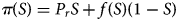
We can illustrate the possible shapes of π(S) as follows. First, consider the case in which some saignée improves profits, so π′(0) > 0.Footnote 9 Then, as described previously, π(S) is initially increasing and concave, and eventually it is convex. This gives rise to two possible shapes, depicted in Panels A and B of Figure 1. In this case, the solution to the winemaker's profit-maximization problem will either be an interior solution, as in Panel A, or a corner solution at S = 1, as in Panel B. Which of these solutions is optimal depends on the price of rosé because at a saignée fraction of one, π(1) = P r. Thus, at S = 1 the heights of the profit curves in Panels A and B are determined by P r. If the rosé price is low relative to the price of the primary wine, the winemaker should choose a small (but positive) saignée fraction (Panel A), but if the rosé price is high, the winemaker should bleed 100% of the juice into rosé, and thus optimally choose S = 1 (Panel B).
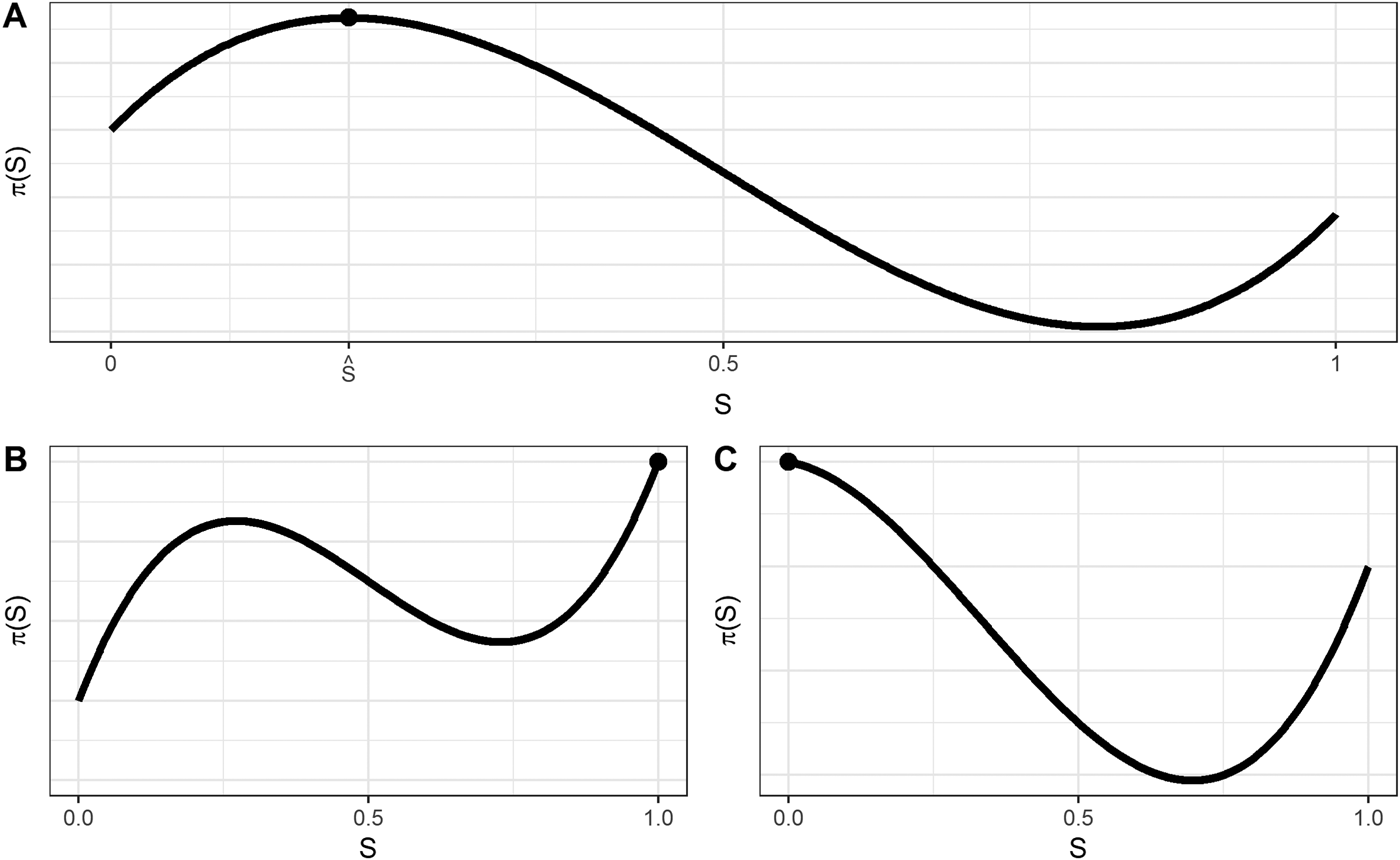
Figure 1. Possible realizations of the profit function, π(S).
Note: The black dot indicates the optimal saignée for each scenario.
But it is also possible that even a small amount of saignée decreases profits, so π′(0) < 0. It turns out that even in this case, π″(0) < 0, the expression is concave (though, in this case, initially decreasing). For larger values of S the profit expression becomes convex and is eventually increasing. This scenario is depicted in Panel C, where the optimal value of saignée is at the corner solution of S = 0. Because profits in the interior region are always below this corner solution, the solution is either to do no saignée, yielding π(0) = f(0), or to make only rosé, yielding π(1) = P r. It turns out, as we will show, that under the assumptions of our model, it is not possible for π(1) > π(0) (when π′(0) < 0, as in Panel C). Thus, if profits are initially decreasing in S, then the optimal value is S = 0.
The solutions depicted in Figure 1 are formalized in Proposition 1. For any given winemaker, there are three candidate levels of saignée. The first candidate is the interior maximum, defined as follows:
Definition 1. The optimal interior value of saignée (denoted  $\hat{S}$) is the value of S ∈ (0, 1) that satisfies both:
 $${\pi\, }^{\prime}( \hat{S}) = P_r-f( \hat{S}) + {\,f}^{\prime}( \hat{S}) ( 1-\hat{S}) = 0$$
 $${\pi\, }^{\prime \prime}( \hat{S}) = {\,f}^{\prime \prime}( \hat{S}) ( 1-\hat{S}) -2{\,f}^{\prime}( \hat{S}) < 0$$
The second and third candidates are S = 0 and S = 1, where the winemaker converts either 0 or 100% of her juice into rosé. No other level of saignée can ever be optimal under this model. The choice between the three candidate solutions turns out to be analytically tractable, and we summarize this as our main result in Proposition 1.
Proposition 1. The optimal saignée fraction is given by:
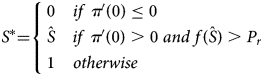 $$S^\ast{ = } \left\{{\matrix{ 0 & {{if}\;{\pi }^{\prime}( 0) \le 0\;\,\;\;\;\;\;\;\;\;\;\;\;\;\;\;\;\;\;\;\;\;} \cr {\hat{S}} & {{if}\;{\pi }^{\prime}( 0) > 0\;{and}\;f( \hat{S}) > P_r} \cr 1 & {{otherwise}\;\;\;\;\;\;\;\;\;\;\;\;\;\;\;\;\;\;\;\;\;\,\;\;\;\;} \cr } } \right.$$
Proof. We will make use of three results on the shape of π(S). First, recall that π″(0) = f″(0) − 2f′(0) < 0, where the inequality holds by Assumptions 1 and 2. Second, recall that π″(1) = −2f′(1) > 0, where the inequality holds by Assumption 3. Thus, π(S) is always concave for sufficiently small S and convex for sufficiently large S. Third, we note that π′(1) = P r − f(1) > 0, where the inequality holds by Assumption 4; so π(S) is eventually increasing in S.
The rest of the proof hinges on the slope of π(S) at S = 0: π′(0) = P r − f(0) + f′(0), which is clearly positive if P r > f(0) (after invoking Assumption 1), but can be negative if P r < f(0). Whether it is positive or negative depends only on the primitives of the problem (the shape of f(S) and P r). We take each case in turn.
If π′(0) > 0 (which can be regarded as the typical case, depicted in Panels A and B of Figure 1), then π(S) is initially increasing and concave and eventually convex, which implies that the interior maximum  $\hat{S}$ exists and therefore that $S = \hat{S}$ delivers higher profit than S = 0. Whether $S = \hat{S}$ delivers higher profit than S = 1 depends on $\pi ( \hat{S}) {\rm \mathbin{\lower.3ex\hbox{$\buildrel \\ \vskip-0.1pc < \over {\smash{\scriptstyle> }\vphantom{_x}}$}}\ }\pi ( 1) $, that is,
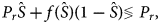 $$P_r\hat{S} + f( \hat{S}) ( 1-\hat{S}) {\rm \mathbin{\lower.3ex\hbox{$\buildrel\\\vskip-0.1pc< \over {\smash{\scriptstyle> }\vphantom{_x}}$}}\ }P_r, \;$$
which reduces to the inequality  $f( \hat{S}) {\rm \mathbin{\lower.3ex\hbox{$\buildrel\\\vskip-0.1pc< \over {\smash{\scriptstyle> }\vphantom{_x}}$}}\ }P_r$. So if π′(0) > 0, then $S ^\ast\;{ = }\; \hat{S}$ if $f( \hat{S}) > P_r$ and S* = 1 if $f( \hat{S}) < P_r$.
Instead, if π′(0) ≤ 0 (depicted in Panel C of Figure 1), then π(S) is initially decreasing and concave and eventually becomes convex, which implies that  $\hat{S}$ does not exist so the solution must be at a corner of 0 or 1. Whether S = 0 delivers higher profit than S = 1 depends on $f( 0) \lessgtr P_r$. However, the fact that π′(0) < 0 implies that f(0) > P r (because π′(0) = P r − f(0) + f′(0) and f′(0) ≥ 0 by Assumption 1). Thus, we conclude that if π′(0) ≤ 0 the optimal value of saignée must be S* = 0.
Proposition 1 emphasizes the importance of the price of rosé (P r) in determining the optimal saignée fraction. Because π(1) = P r, it is easy to see P r in Figure 1 (it is the height of the curve at S = 1). When the price of rosé is relatively low (Panels A and C), then the optimal saignée choice is either at the interior solution  $S = \hat{S}$ or at S = 0. The second case is obtained when even conducting a small amount of saignée lowers profits. This is the outcome we typically observe for producers of premium red wines, such as first-growth Bordeaux wines, which presumably practice very little saignée.
However, when the rosé price is sufficiently high (Panel B), then the corner solution at S = 1 prevails and only rosé is produced. We do not necessarily regard this case as unusual. Consider a winery for which only relatively low-quality (and thus low-priced) primary wine could be produced. Even though a little saignée would improve the price of the primary wine, it pays to convert all juice to rosé (see Panel B).
For many wineries, particularly those that intend to utilize saignée to increase the quality of their primary wine, the optimal solution will be the interior one ( $\hat{S}) $, depicted in Panel A of Figure 1. What can be said about the magnitude of $\hat{S}$? Consider first the intuitively appealing strategy of choosing S to maximize the price of the primary wine (so $S = \bar{S}$, which maximizes f(S)). How does $\bar{S}$ compare to $\hat{S}$? Provided that the interior maximum exists (the necessary and sufficient condition is that π′(0) > 0), we can show that it is never strictly optimal to choose $\bar{S}$, regardless of the functional forms or parameters of this problem. Proposition 2 summarizes this result.
Proposition 2. Let  $\bar{S}$ be the interior saignée fraction that maximizes the quality of the primary wine. The interior optimal saignée fraction is always smaller than this value: $\hat{S} < \bar{S}$.
Proof. Marginal profit at  $\bar{S}$ is ${\pi }^{\prime}( \bar{S}) = P_r-f( \bar{S}) $, whose sign depends on $P_r\lessgtr f( \bar{S}) $. This expression can be immediately signed as:
 $$f( \bar{S}) > f( \hat{S}) > P_r$$
 The first inequality follows from the definition of  $\bar{S}$ (which maximizes f(S) so no other value of S could return a higher f(S)). The second inequality follows from Proposition 1, which implies that $\hat{S}$ exists and is optimal if and only if π′(0) > 0 and $f( \hat{S}) > P_r$. Thus, $f( \bar{S}) > P_r$, which means that marginal profit at $\bar{S}$ is decreasing, so $\hat{S} < \bar{S}$.
Thus, we can safely rule out the intuitively appealing result that the quality-maximizing fraction of saignée is also the profit-maximizing fraction of saignée. Indeed, when a positive amount of saignée is warranted, it is always optimal to either choose a lower level of saignée (Panel A) or to specialize only in rosé and set S = 1 (Panel B).
We can also use this model to ask how a winemaker should respond to an exogenous shift in the price of rosé. Demand for rosé has risen sharply in recent years, raising the possibility that P r has increased. It is straightforward to show that, when the optimal value of saignée is in the interior, a higher rosé price always leads to more saignée.
Proposition 3. A higher price of rosé always leads to a higher interior optimal saignée fraction:
 $$\displaystyle{{d\hat{S}} \over {dP_r}} > 0$$
Proof. Totally differentiate Equation (7) with respect to P r and S to get:
 $$\displaystyle{{d\hat{S}} \over {dP_r}} = \displaystyle{{-1} \over {SOC}}$$
Where SOC refers to the second-order condition for the revenue maximization problem, which is always negative for the interior solution identified earlier (see Definition 1).
Finally, we can use the model to analyze the question of whether to saignée at all. According to Proposition 1, there is a very specific set of circumstances under which S* = 0. In particular, this occurs when π′(0) < 0, so the winemaker experiences a drop in profit from even a small amount of saignée. A necessary condition for this to arise is that f(0) > P r: the price of a zero-saignée bottle of primary wine is greater than the price of a bottle of rosé. If f(0) > P r, then it might be the case that S* = 0. However, this condition is not sufficient because if f′(0) is large, then even when f(0) > P r, π′(0) > 0, and it will be optimal to engage in at least some saignée.
III. Simulations
To illustrate these results and characterize the winemaker's choice of the optimal saignée fraction, we parameterize the model using plausible values of the relevant parameters and conduct a series of structural simulations. Let the exogenous price of rosé (P r) range from $0 to $50 and assume that the price of primary wine is quadratic in S:
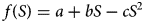 $$f( S) = a + bS-cS^2$$
for positive constants a, b, and c. For this simulation, we use a = 20, b = 80, and c = 160, which produces the price function shown in Figure 2 and satisfies Assumptions 1–4. Under this model, the quality-maximizing saignée fraction is  $\bar{S} = {b \over {2c}} = 25$%, and delivers a quality-maximizing primary wine price of $f( \bar{S}) = a + {{b^2} \over {4c}} = \,$$30.
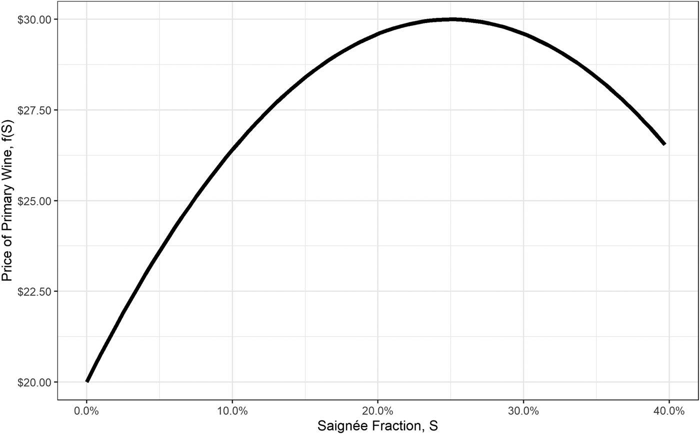
Figure 2. Primary wine price as a function of saignée percentage (S) in our simulations.
The relationship between total revenues and the saignée fraction depends on the price of rosé wine, as shown in Figure 3. Naturally, the higher the price of rosé wine, the higher the optimal saignée fraction. As discussed earlier, even when the price of rosé wine is 0, the optimal saignée fraction can be greater than zero (it is around 15% in the simulation), and maximized revenues grow with the price of rosé wine. When the price of rosé exceeds the maximum value of the primary wine (here, $30), the optimal saignée jumps suddenly to 1.
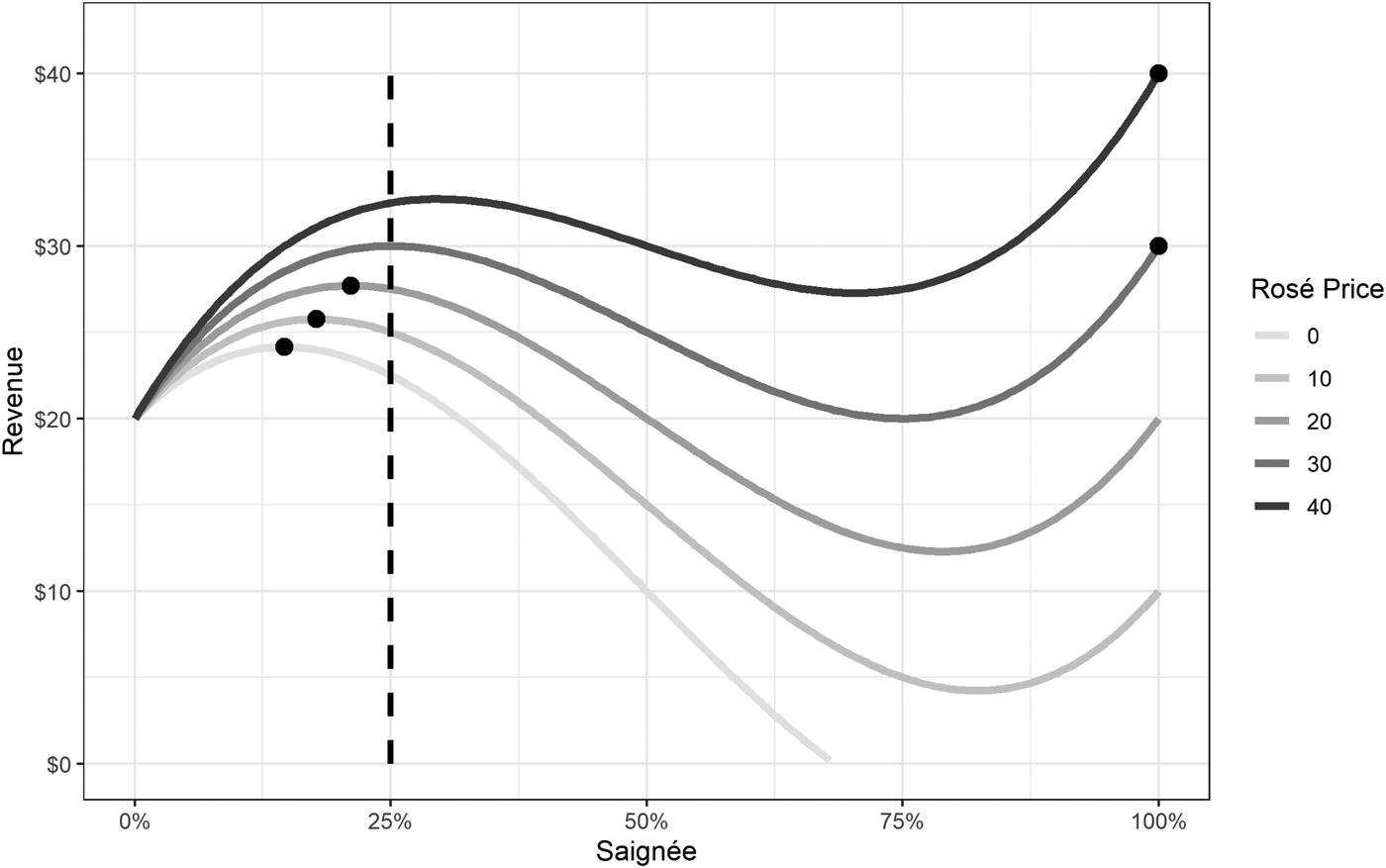
Figure 3. Revenue and optimal saignée.
Notes: Solid lines indicate revenue as a function of S. Dashed line shows the level of saignée that maximizes wine quality ( $\bar{S}$). Dots show optimal saignée for each rosé price.
Finally, the profit-maximizing saignée percent as a function of the rosé price is given in Figure 4. The relationship is increasing and monotonic, as stated in Proposition 3. When the price of rosé exceeds the maximum value of primary wine ($30), optimal saignee jumps to 1.
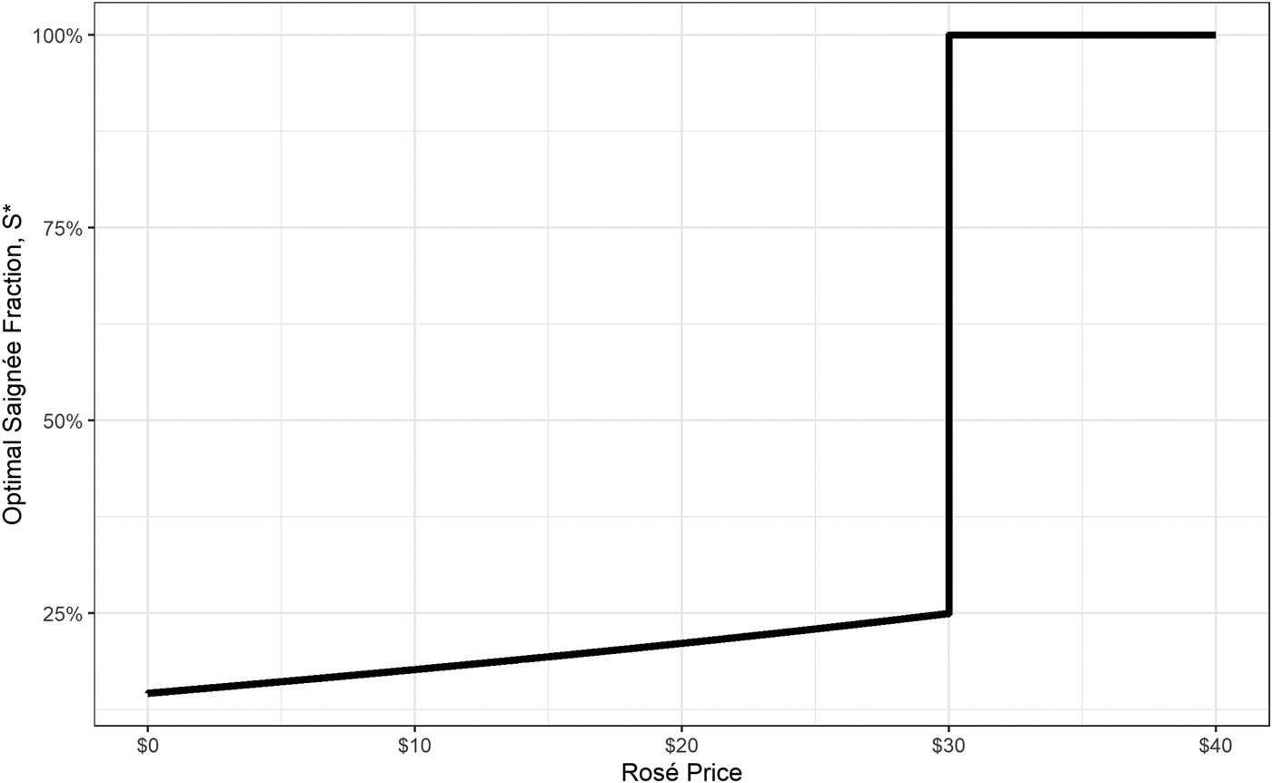
Figure 4. Optimal saignée as a function of rosé price.
IV. Conclusion
Much has been written by oenologists about the practice of saignée, which concentrates flavor and raises the quality (and price) of some primary wines. While that literature is enlightening about how to optimize saignée for wine quality, we observe that increasing the level of saignée also induces interesting economic tradeoffs for the winemaker. On one hand, she concentrates flavor and may raise the value of her primary wine, but she also produces a valuable rosé byproduct and loses some of her primary wine volume. To the best of our knowledge, these tradeoffs have not been carefully explored. We develop and analyze a model that we believe is the first theoretical treatment of the economics of saignée.
Our main result is that there are only three possible levels of optimal saignée for any winemaker. It can be zero, a relatively low but interior value, or one. The first case (S* = 0) arises when the primary wine is extremely valuable (relative to rosé) and the quality of that wine sees little or no improvement from small amounts of saignée. The second case (S* = interior at  $\hat{S}$) arises when a little saignee raises profits, but the price of rosé is not too high. In this case, a winemaker will need to fine-tune the level of saignée, but importantly, will always optimally choose a value of saignée that is less than the quality-maximizing amount (Proposition 2). The third possibility is that S* = 1, so all juice is converted into rosé. This case arises when the price of rosé is sufficiently high, and the quality (and price) of primary wine is relatively low.
These results help to explain observed differences in saignée practices across wine grape varietals around the world. Saignée is relatively uncommon for premium red wines made from cabernet sauvignon and merlot. As these wines tend to be already concentrated, the gain in quality from saignée is unlikely to offset the loss in primary wine production, even accounting for the sale of rosé. Our model shows that the optimal saignée fraction in this case is zero. On the other hand, saignée may provide larger gains in the quality of wines made from lighter-skinned grapes like grenache and pinot noir, and indeed, we see that saignée is more common for these varietals. However, our model makes clear that a positive effect of saignée on wine quality (f′(0) > 0) does not guarantee that a positive amount of saignée is optimal because it can still be the case that π′(0) < 0. If the loss in the value of primary wine production is sufficiently high, then the optimal saignée fraction is again zero. The model also helps to rationalize why some wineries specialize in rosé. If the quality of their primary wine is modest, even when fine-tuning saignée, but they can access a relatively high price of rosé, then it is optimal to produce 100% of the juice into rosé, as is sometimes the case in certain wine-producing regions, such as Provence.
There are broader implications of this paper for winemaking. A natural extension of our work would be to study the economic implications of wine-blending practices, whereby wine from multiple varietals is blended post-fermentation to produce a primary wine. For example, many wines from the Bordeaux region in France blend cabernet sauvignon, merlot, cabernet franc, and smaller amounts of malbec and petite verdot. The results in this paper suggest that in some cases, the profit-maximizing blend of various varietal wines may differ from the blending ratio that produces the best primary wine.
Acknowledgments
We thank two anonymous referees and our editor, Karl Storchmann, for their assistance with this manuscript. We thank Ivory Tower Wines and Dierberg/Star Lane for providing inspiration for this study. Competing interests: Christopher Costello, Olivier Deschênes, Charles Kolstad, and Andrew Plantinga declare no competing interests. Tyler Thomas is president and head winemaker at Star Lane and Dierberg Vineyards.


 Open access