


I. Introduction
The potential price appreciation in wine investment is contested both among researchers and investors. Of course, a seasoned wine trader might have excellent returns with a simple buy-low-sell-high approach by hunting for outliers at auction. In analyzing investment potential, this research seeks to enhance the measurement of price appreciation with the age of the wine and create a measurement of wine markets that have been normalized for wine aging. A wine label refers to any bottle of wine as identified by brand and vintage. The analysis of a single label, such as the work by Jovanovic (Reference Jovanovic2008) studying 1870 Lafite, cannot distinguish the market and aging effects on the price at auction. Rather, a broad dataset covering a range of labels observed over many calendar dates is necessary.
This research was motivated by the observation that the distribution of wine labels traded in the first decade since their release is different from the wine labels traded several decades after their release. If all wines from a region are analyzed together, then one would observe that lower-priced wine labels drop out of the data set with age sooner than higher-priced wines. This bias in the data distribution is referred to as right-censoring in the survival modeling literature, and when the censoring is selective based upon an unmodeled variable, it can lead to a bias in estimating the function versus age, which is referred to as frailty (Balan and Putter, Reference Balan and Putter2020) when the bias is due to an unobserved explanatory variable. In this research, we hypothesize that trading frequency (popularity) can be used as a segmentation variable to eliminate frailty in the estimates.
In a continuation of our previous research into applying Age-Period-Cohort (APC) analysis to wine prices (Breeden and Liang, Reference Breeden and Liang2017; Breeden, Reference Breeden2010), we explored the impact of market segmentation on the estimation of wine investment returns. Specifically, this was done by performing separate APC analyses on different wine segmentations, specifically estimating the wine market and price growth with wine age. Analyzing data from Bordeaux, Italy, Australia, and California, we examined how the same segmentation approach performed in each region.
This analysis will show that measurements of the wine market are remarkably stable relative to the segmentation scheme chosen, but price appreciation with age varies strongly depending upon how one defines the segments. With the cause appearing to be due to data censoring for less popular wines, we developed a forward-looking segmentation algorithm that predicts future popularity so that even young wines may be properly segmented in order to reduce bias due to censoring. Further, comparisons across regions not only provide a useful cross-validation of the approach but also provide market and price appreciation with age that are not well studied outside Bordeaux.
This paper proceeds as follows: Section II provides a literature review on wine as an investment. Section III describes the data used in the study. Section IV describes the APC approach for estimating market trends and price growth with the age of a wine. Section V provides all of the results by region studied, and Section VI describes our conclusions.
II. Wine investment literature
The ultimate goal of this research is to predict future returns on investing in a specific wine or portfolio of wines. The earliest analysis of wine prices was by Ashenfelter (Reference Ashenfelter2010). Wood and Anderson (Reference Wood and Anderson2006) employed a cubic age function and demonstrated that the age of a wine was predictive of price. Various authors have studied the rate of return for holding wines and the diversification benefit of having wine as part of an overall portfolio. See Storchmann (Reference Storchmann2012) for a detailed survey of the literature.
With a wine-only portfolio, one hopes that wines have a higher rate of return than other investments (Burton and Jacobsen, Reference Burton and Jacobsen2001; Fogarty, Reference Fogarty2006; Jaeger, Reference Jaeger1981; Krasker, Reference Krasker1979; Jones and Storchmann, Reference Jones and Storchmann2001), although not all studies have found long-term positive returns. More recently, Sanning, Shaffer, and Sharratt (Reference Sanning, Shaffer and Sharratt2008) show that wine has exhibited large excess returns. However, any study conducted immediately prior to the 2011 wine market correction is likely to be overly optimistic. As with most markets, one must consider long periods in order to capture both rallies and corrections.
With a diversification approach (Bouri et al., Reference Bouri, Gupta, Wong and Zhu2018; Chu Reference Chu2014), a lower-return series that is somewhat uncorrelated to other investment vehicles is also beneficial. So, any return modestly greater than zero could be beneficial if uncorrelated or, better yet, anti-correlated to other instruments. Initial studies did find low or negative correlation to typical investment vehicles (Fogarty, Reference Fogarty2010; Masset and Henderson, Reference Masset and Henderson2010; Masset and Weisskopf, Reference Masset, Weisskopf, Ashenfelter, Gergaud, Storchmann and Ziemba2018; Sanning, Shaffer, and Sharratt, Reference Sanning, Shaffer and Sharratt2008), but intrinsic return remains a question.
Fogarty and Sadler (Reference Fogarty and Sadler2014, table 1) summarize previous studies, appropriately concluding that researchers have obtained a wide variety of results depending upon the time period examined and the method of analysis applied. The preponderance of the literature appears to take a portfolio perspective where one presumably has a diverse collection of wines of many ages so that only the overall market matters. However, if all wine prices increase with age or at least do not decrease throughout the tradable life of a wine, then there is an inherent price growth rate of the portfolio separate from the market. The only way to purely measure market trends for a portfolio of wines would be to steadily replace older labels with newer labels such that the average age remains stable.
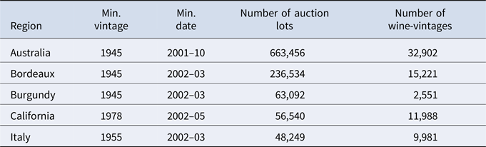
Table 1. Summary of the data used for analysis
III. Data
The current study leverages wine prices from AuctionForecast.com. Table 1 provides a summary of the date and vintage ranges for the analysis by segment, as well as the number of auction lots and wine-vintages. In all usages, vintage refers to the year the grapes were grown.
The data was collected from Acker Wines, Bidforwine, Bonhams, Christie's, Chicago Wine Company, Hart Davis Hart, Langton's, Skinner, Sotheby's, Spectrum, Veiling Sylvie's, and Zachy's. Only prices from homogenous lots were retained, meaning the lot price pertains to a single wine-vintage and bottle size. The lot price was divided by the number of bottles in the lot, and all prices were converted from the original auction currency to U.S. dollars using the exchange rate on the date the auction was held. Only standard 750 ml bottles were retained for the analysis.
IV. Analysis methods
Since the primary goal of this analysis is to distinguish market trends from price appreciation due to wine maturation, APC models are a natural approach. APC models were designed to decompose cohort (or in this case, wine-vintage) performance data into three constituent functions: a lifecycle function F(a) of age a of the wine-vintage, a quality adjustment function G(v) of vintage v (the year recorded as vintage on the bottle being sold), and an environment (market) function H(t) of calendar date t. In the case of modeling auction prices p(i, a, v, t) for label i, this can be expressed as

where G(v) is an overall quality adjustment relative to the vintage year. The analysis can be further segmented as G(i, v), a quality adjustment for a specific label, if enough data exists for each label i.
APC models are well-suited to the current analysis because they emphasize estimating the nonlinear structure of the functions of age and calendar date, which is key to understanding the long-term potential for appreciation in wine prices. Linear or low-order polynomial functions of age do not provide the resolution necessary to draw meaningful conclusions about lifecycle and market impacts upon price appreciation.
The quality adjustments for a vintage year or a specific label are assumed to be constant adjustments relative to lifecycle and market. As such, a detailed analysis of the explanatory factors behind these adjustments, although interesting, is not relevant for the current analysis.
The estimation can be performed with spline approximations of the functions using maximum likelihood estimation (Mason and Fienberg, Reference Mason and Fienberg1985; Holford, Reference Holford1983, Reference Holford, Everitt and Howell2005) or via a Bayesian estimation of the functions represented nonparametrically with one parameter at each point in age, vintage, and calendar date (Schimd and Held, Reference Schmid and Held2007). A Bayesian estimation approach was employed here because it avoids the premature smoothing of spline estimation and polynomial runaway in the tails of the functions where the data becomes thin. The use of APC models for analyzing wine auction prices has been previously described by Breeden and Liang (Reference Breeden and Liang2017).
APC models may be understood as a specific kind of panel regression, where wine-vintages are observed repeatedly via auction lot prices. APC models can also be described within the context of hedonic regression (Rosen, Reference Rosen1974). The APC modeling technique is also similar to Repeat Sales Regression (Bailey, Muth, and Nourse, Reference Bailey, Muth and Nourse1963), although APC in this research is being applied to analyzing prices directly rather than price changes because the data density is very nonuniform with time.
APC analysis of wine data is most similar to the research of Dimson, Rousseau, and Spaenjers (Reference Dimson, Rousseau and Spaenjers2015), who examine the impact of aging on wine prices and by using a value-weighted arithmetic repeat-sales regression over 1900–2012, examining the long-term return for vintages of Haut-Brion, Lafite-Rothschild, Latour, Margaux, and Mouton-Rothschild. They looked for price appreciation due to lifecycle with wine age, environmental impacts with a calendar date, and included production and quality as explanatory variables to explain vintage variation.
We begin by applying APC models to auction price data by region to show overall appreciation for age and market changes. Previous research (Breeden, Leonova, and Bellotti, Reference Breeden, Leonova and Bellotti2021) has shown that data with age, vintage, and time effects cannot be modeled without either a linear function ambiguity as with APC models or a multicolinearity problem as with regression and Cox PH models. For this analysis, the vintage function was assumed to have no net linear component, which implies that all long-term price appreciation will appear either in the market function or lifecycle function.
To explore segmented analysis, the APC models are applied to the trade volume for each label to measure the expected frequency of trades versus age and normalized for the overall data volume by calendar date. This allows us to predict the lifetime trading popularity of a wine very early in its age. The wines in each region are then segmented based upon historic and predicted popularity to re-estimate price appreciation via a popularity-segmented APC analysis within each region.
A. Results without segmentation
The first step in the analysis was to create a baseline for comparison by performing APC analysis on all available auction data within each region for labels with enough trades for analysis. Figure 1 shows the resulting price appreciation lifecycles versus the age of wine in years. The Bayesian APC approach was employed, so the results have no smoothing. For use in forecasting for portfolio management, one would prefer to smooth these functions, guided by the confidence intervals shown as shaded regions.
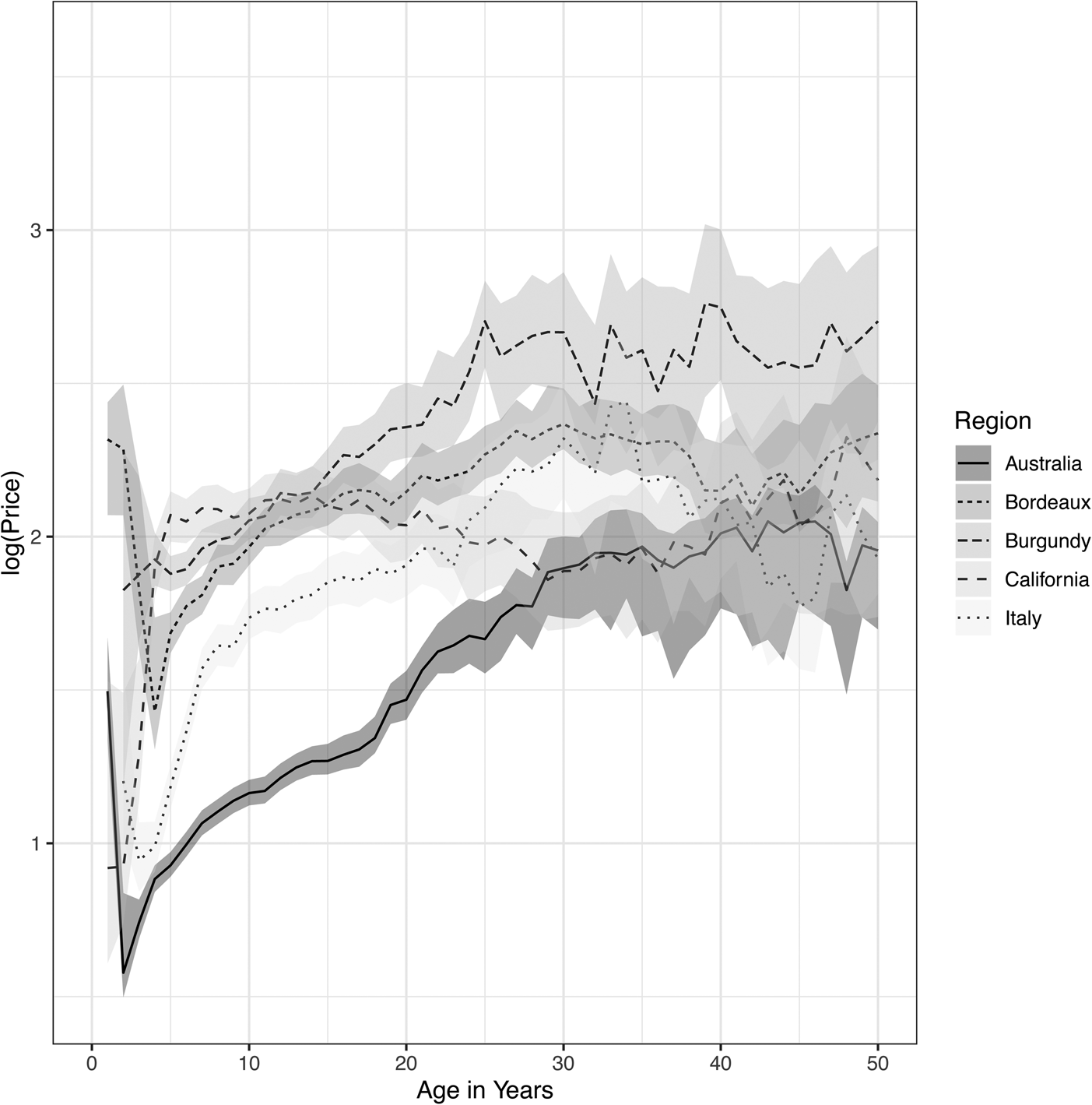
Figure 1. Price appreciation lifecycles from APC analysis, showing the average log10(price) for red wine versus age for each region.
The wines of most regions show an initial drop in price followed by a long-term appreciation over the subsequent 20 to 30 years before the prices flatten out. The results are shown on a log scale to make the dynamics more visible.
The market trends from the APC analysis by region are shown in Figure 2 with January 2010 normalized to 100. The original environmental functions H(t) were measured on a log scale, so the market index is computed as exp (H(t)). The confidence intervals were not plotted in order to simplify the visual presentation, but they can be inferred from the variation in the graphs.
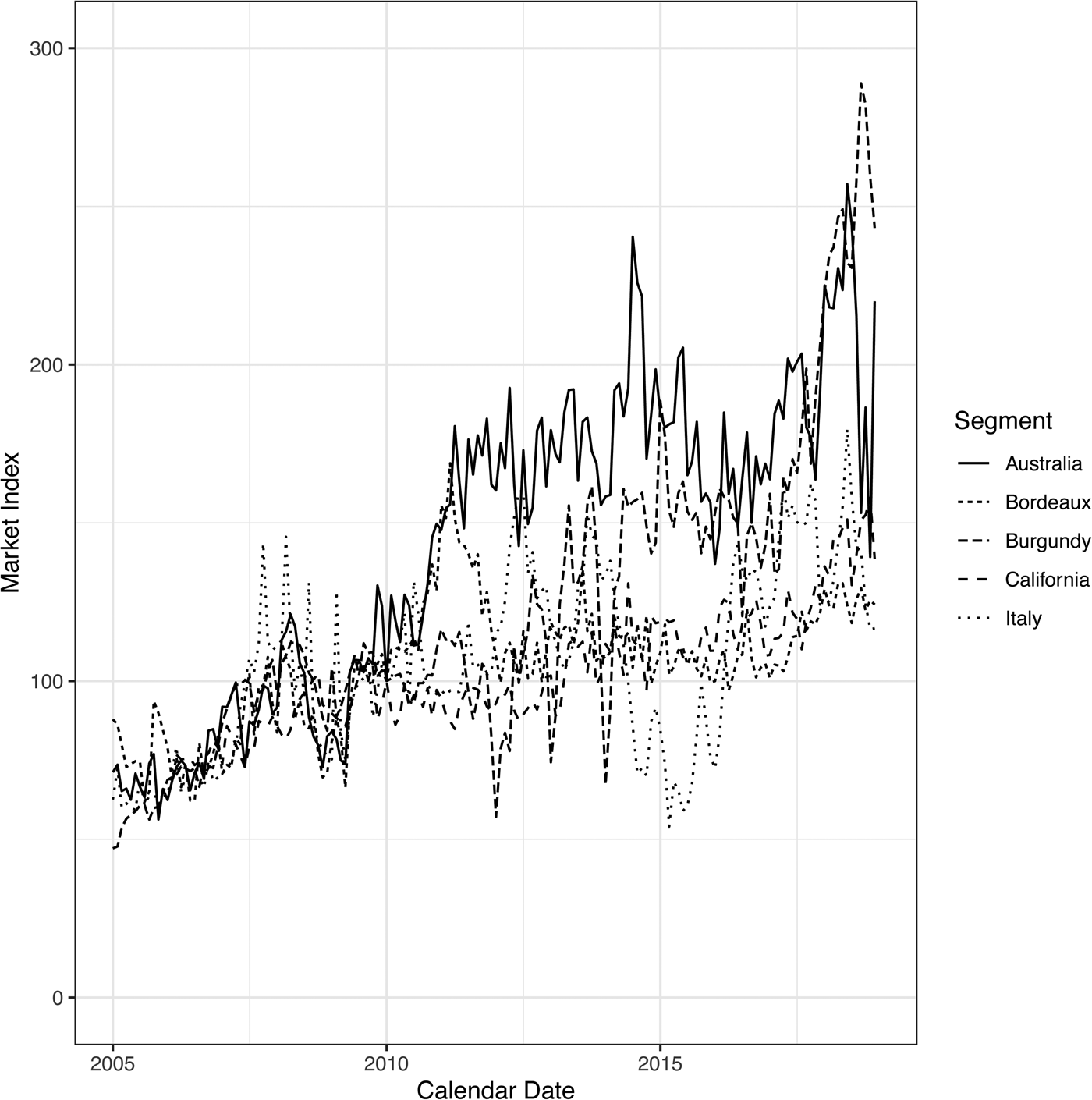
Figure 2. Market price indices from APC analysis for red wines from each region versus calendar date (monthly).
Some features of the graphs agree with intuition. The “Lafite Bubble” of 2011–2012 really affected all Bordeaux wines and can be seen here as a dramatic boom-bust cycle. Throughout 2017–2019, a dramatic increase in Burgundy is apparent, but without a market collapse so far. Australian wines have been in a trading range since 2012, which can nevertheless be profitable for active investors. Italian wines have seen fewer significant booms and busts, while Californian wines have been much less volatile than the others, except for a period of appreciation beginning in 2018.
Analysis of many candidate segmentations shows that the market estimates are very robust within a region. If we just measure the market appreciation across the full 14-year period, the result can be susceptible to recent increases, such as with Burgundy and California. As an alternative, we computed the mean one-year market return and confidence interval, to show how volatile the market can be. A buy-and-hold strategy in this kind of market could be problematic, but volatility creates opportunities for an active trader.
Table 2 shows the market returns from January 2005 through December 2018, a 14-year span, as well as the average one-year return starting from any month in that series, and the 95% confidence interval about the mean. All of the returns are statistically significant over this period.
Table 2. Investment returns realized from the market indices in Figure 2

Note that compounding the annual return over 14 years would be dramatically higher than the observed returns from 2005 through 2018 because wine returns are strongly anticorrelated over 12 to 24 months, which is a reflection of the boom-bust cycles observed in Figure 2.
B. Modeling wine-vintage popularity
As we explored segmenting the analysis within regions, we considered segmenting by wines with the highest initial price, from the most popular vintages and those most commonly selected in wine market baskets. All of these approaches have serious flaws. Initial price sales indicate little about long-term appreciation. Not all wines of a given vintage have the same potential for appreciation. Wines in popular market baskets are generally older and thus are not useful for understanding the appreciation potential of newer vintages.
After discussions with industry experts and dissatisfaction with the test results for the methods mentioned previously, we looked at predicting label popularity so that labels can be segmented very early in their lifecycles for the proper estimation of their appreciation value. This was done by creating an APC model for the trading frequency of labels by estimating the trading volume versus the age of the label and trading volume by calendar date. Then, the popularity of each label, G P(i, v), is estimated as a one-parameter regression with lifecycle F P(a) and environment H P(t) as fixed inputs.

In absolute terms, the lifecycle and environment reflect the density of our training data. The analysis is more insightful when measured relative to the total volume of data. Figure 3 shows these normalized lifecycles—this time with age measured monthly rather than annually, so that the variation within the year is clear. These results show that the rate of increase and decrease are quite similar across regions, except for Bordeaux, which has a significantly higher long-term trading frequency.
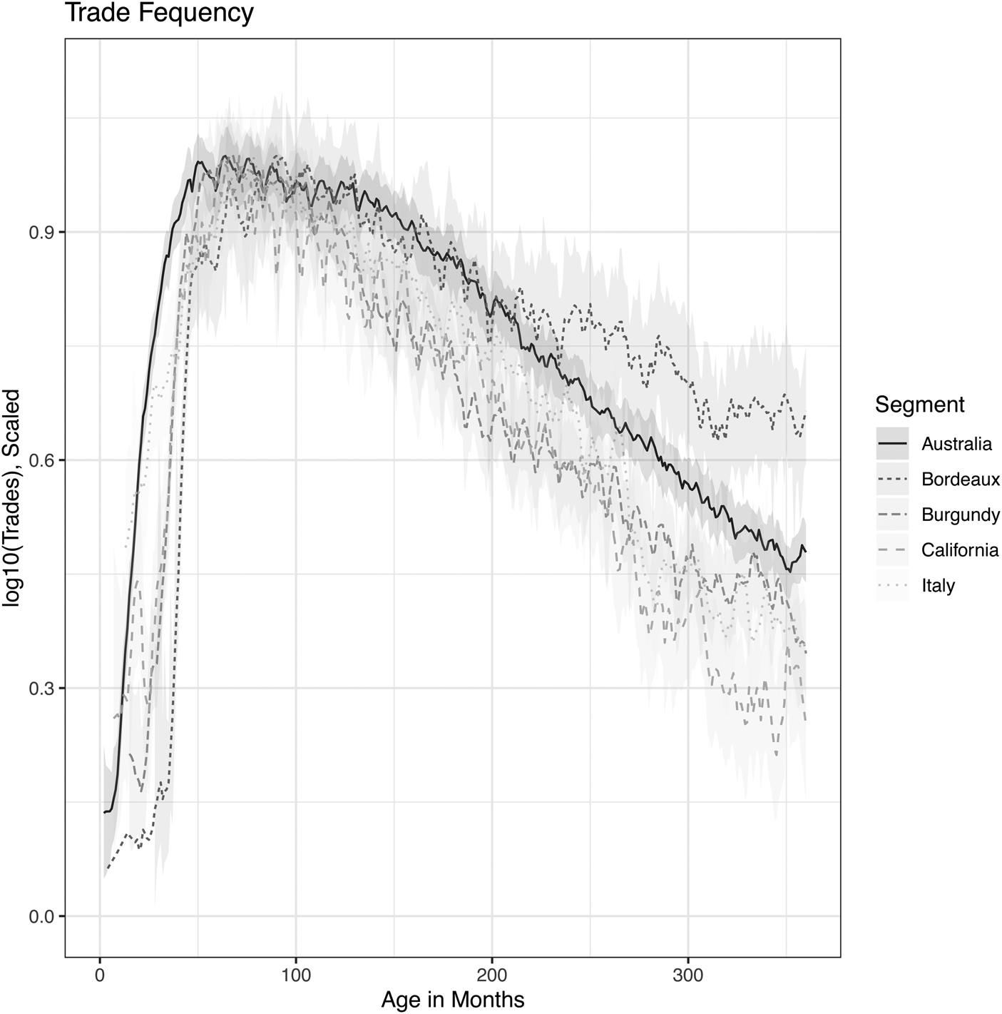
Figure 3. Lifecycles for trading volume versus age of a label. The original estimate was the log of trading volume, which was scaled for this graph between 0 and 1 to normalize for the differing data density between regions.
C. Results with segmentation by popularity
The value of the popularity analysis is that the label popularity G P(i, v) can be estimated for any age and allows us to create segments with wines of different ages. Within each region, we created four segments based upon ranking the popularity: 1–25, 26–100, 101–500, and 501+. With these segments, the APC analysis of log(price) was rerun for each region, as shown in Figure 4 through Figure 8.
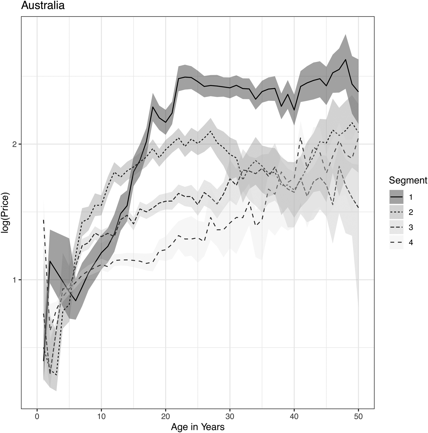
Figure 4. Price lifecycles for Australian wines as obtained from a Bayesian APC analysis applied to segmentation by popularity tiers.
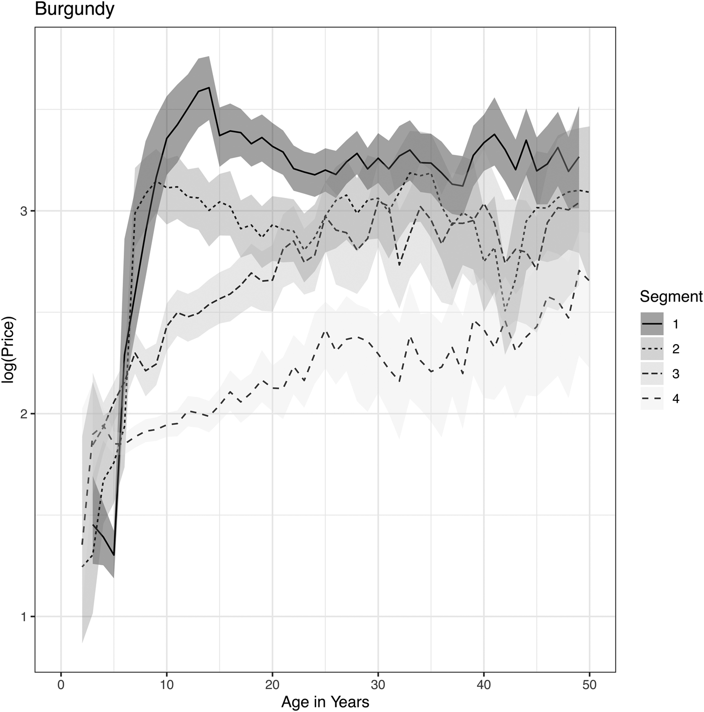
Figure 5. Price lifecycles for Bordeaux wines as obtained from a Bayesian APC analysis applied to segmentation by popularity tiers.
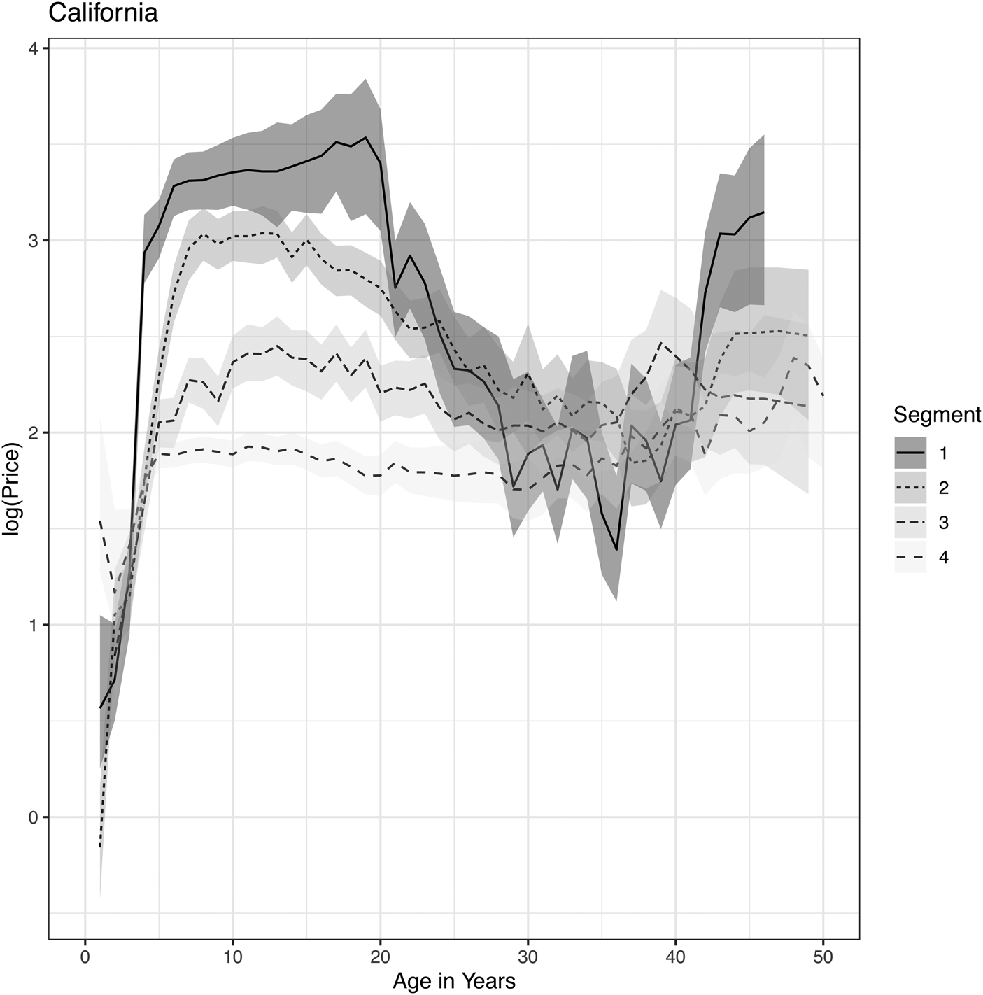
Figure 6. Price lifecycles for Burgundy wines as obtained from a Bayesian APC analysis applied to segmentation by popularity tiers.
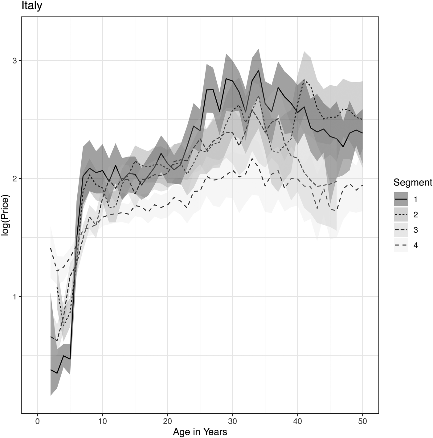
Figure 7. Price lifecycles for California wines as obtained from a Bayesian APC analysis applied to segmentation by popularity tiers.
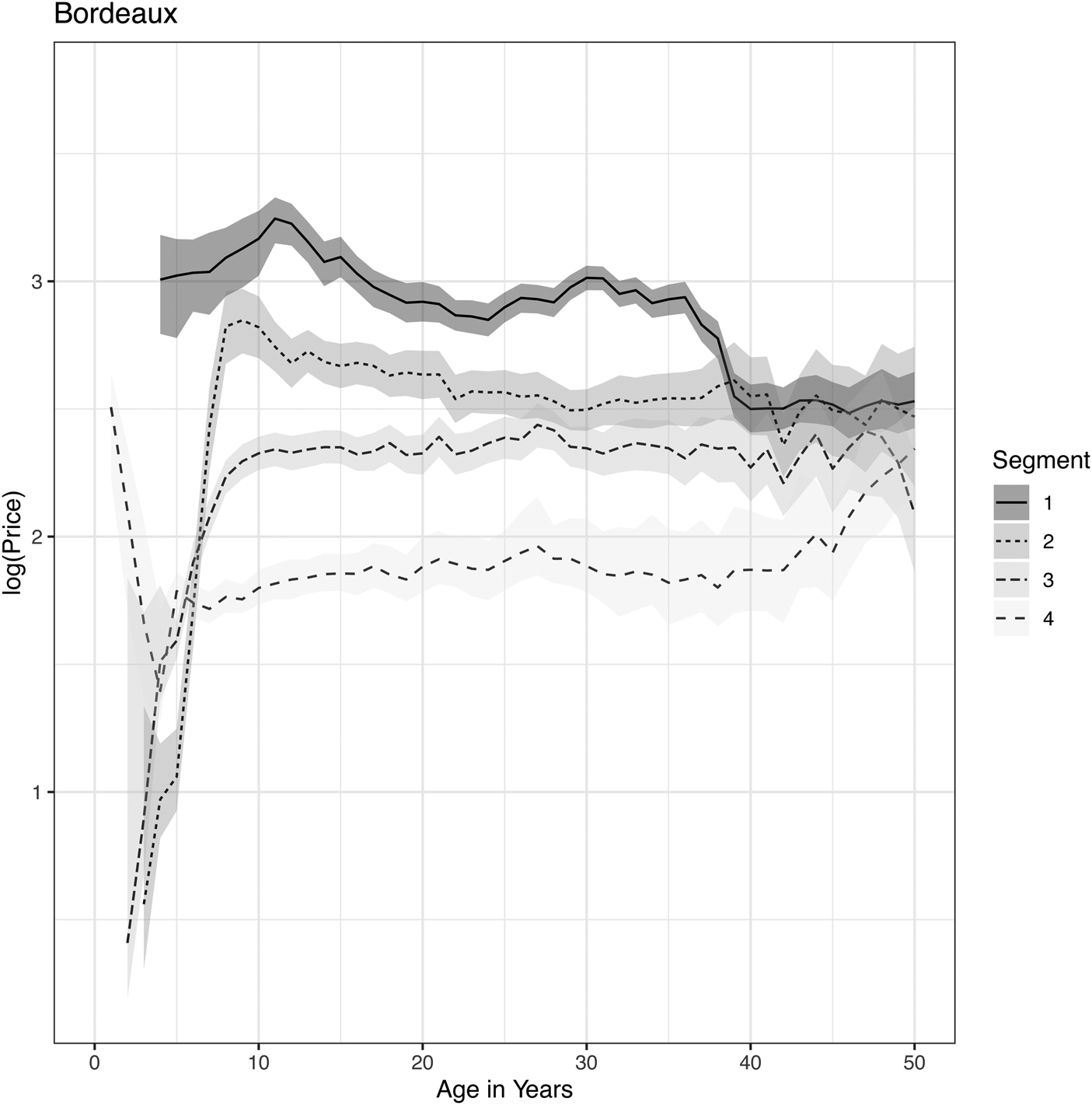
Figure 8. Price lifecycles for Italian wines as obtained from a Bayesian APC analysis applied to segmentation by popularity tiers.
To glean insights from these results, compare the segmented region analysis to the unsegmented result in Figure 1. Australia is an anomaly compared to the other regions. Starting with Bordeaux, because those wines are the most popular for investors, the top 25 wines immediately begin with high prices. Prices peak around age 12 and then are largely flat thereafter. The second and third-tier wines rapidly increase in price over the first ten years and then flatten out. This analysis reveals that the perceived increase in price with the age of the vintage in Figure 1 is due to a selection bias. As wines aged, the higher-priced wines continued to be traded, whereas the less expensive wines did not. Therefore, the buy-and-hold strategy does not guarantee profits for Bordeaux wines and has been largely just an illusion due to selection bias.
The same effect can be seen in Burgundy wines. Tier 1 and 2 both increase rapidly in price for the first 10 years and then flatten out, considering the confidence intervals. Tiers 3 and 4 show a continued increase, but one must question whether this is due to a selection bias again. We cannot further segment the analysis for the less popular wines because the data is quickly exhausted. However, since tiers 1 and 2 are the primary wines for trading, the result is the same as for Bordeaux. Namely, price appreciation with age is not reliable, and the observed increases are better explained as an overall increase in the market for Bordeaux and Burgundy wines. The common perception was that appreciation with age was more reliable than market increases because of past boom-bust events in the market. This analysis shows no reliable increases with age, and investors must assume that all gains are susceptible to future market crashes.
Californian and Italian wines largely continue the pattern just observed. Prices in these markets may peak even earlier, such as at 8 to 10 years of age, and flatten from there. The data in both markets become sparser and more volatile after 20 years, so it may be prudent to assume that prices are mostly flat thereafter.
Lastly, returning to Australia, we see a fundamentally different pattern. Only in this region do prices continue to rise for 20 to 30 years. Still, the top 25 wines plateau first, but the rise is longer than in other regions. Although Wood and Anderson (Reference Wood and Anderson2006) also analyzed Australian wine price appreciation, their analysis focused primarily on growth conditions such as rainfall, temperature, sun, etc. Their predictive factors relative to age are considered only in linear, squared, and cubed terms. Such a low-order polynomial representation will not capture the nonlinear structure being studied here and will be unstable in the high-age tails of the function. As such, the current results reveal a structure not previously observed.
V. Conclusion
Assessing investment returns for wine is challenging because of the complex dynamics of wine prices and the numerous selection biases in the available data. Simple average wine indices can be deeply misleading, as recognized by previous researchers who have sought to tease apart the various drivers from auction results.
The present analysis provides a study of how selection biases may be driving spurious results in assessing wine investment returns. In addition, we found that segmenting by wine popularity is helpful in stabilizing the analysis.
Acknowledgments
The author would like to thank Karl Storchmann (the editor) and an anonymous reviewer for their helpful comments and encouragement.


 Open access