


ELWOOD: “… what kind of music do you usually have here?”
CLAIRE: “Oh, we got both kinds. We got country, and western.”
— The Blues Brothers, 1980I. Introduction
Product differentiation has emerged as a central theme in modern industrial organization. Strong market forces are behind the proliferation of product varieties. On the demand side, consumer heterogeneity plays a major role, with individual choices reflecting differences in underlying tastes and preferences as well as in consumers’ income. On the supply side, product differentiation is a powerful tool for firms to soften the adverse profit consequences of price competition (Tirole, Reference Tirole1988). Much interest concerns the margins along which firms can profitably differentiate their products, with significant implications for business strategy, industry evolution, and public policy. Product differentiation has long been a distinctive feature of the wine industry. Although interest often centers on quality, along an implied vertical differentiation dimension, it is clear that horizontal differentiation catering to the heterogeneity of consumers is just as relevant. In this paper, we assess the determinants of product differentiation in the U.S. wine industry, with special emphasis on the role of geographic origin of wines.
Wine is a classic example of an experience good where consumers cannot ascertain the quality of the product before consumption (Storchmann, Reference Storchmann2012), which presents a potentially deleterious structural asymmetric information problem (Akerlof, Reference Akerlof1970). Several market mechanisms have emerged to deal with this situation; chief among them is firms’ pursuit of strong brand identities that, by leveraging the notion of reputation, can foster repeat purchases (Shapiro, Reference Shapiro1983). In addition to individual firms’ branding strategies—which are supported by proprietary trademarks and are ubiquitous in most differentiated product markets—the wine industry has also developed a somewhat unique system of geographic origin labeling. This approach is based on France's historic experience with the “appellations” system (Meloni and Swinnen, Reference Meloni and Swinnen2013). The core premise is that major components of a wine's distinctiveness are the specific geo-climatic conditions of its production region, the historic grape varieties that characterize the region, and the traditional local practices of wine producers.
The evidence shows that, indeed, the system of appellations has been effective in ameliorating the market failures of asymmetric information in the French wine industry (e.g., Mèrel, Ortiz-Bobea, and Paroissien, Reference Mérel, Ortiz-Bobea and Paroissien2021). In fact, geographic denominations of origin—essentially, collective labeling mechanisms that complement firms’ own brands (Menapace and Moschini, Reference Menapace and Moschini2012)—have been widely adopted in the European Union, which has institutionalized the associated notion of “terroir” into its food quality policy. The extent to which geographic origin labeling should matter for the rest of the world remains an open question, however, given that major elements of the European wine industry development are not common elsewhere. For example, varieties used to produce European wines are typically inherited as part of the local history (e.g., Sangiovese is used to produce Chianti wines), whereas, in the so-called New World, varieties are deliberately chosen by wine producers under fewer constraints.Footnote 1 In fact, the use of varietals has emerged as a key labeling and marketing tool for U.S., Australian, and South American wines.
A plethora of information is typically found on wine labels—often including brand, grape variety, geographic origin (possibly in the form of an appellation classification), alcohol content, and vintage. These intrinsic attributes, combined with other signals, such as price and expert rating, help consumers make wine choices and increase the likelihood of repeated purchases (Horowitz and Lockshin, Reference Horowitz and Lockshin2002). Assessing the relative importance of such factors remains an active area of research, with implications that range from the design of food quality policies to the promotion and marketing strategies of individual firms. In particular, one can ask to what extent geography per se matters relative to brands (Schamel, Reference Schamel2006), or whether geography is redundant information once variety and brand information are known. The latter concept, in particular, has been articulated as a stylized difference between so-called Old World and New World wine industry strategies (Castriota, Reference Castriota2020).
Somewhat in contrast with the accepted view that collective designation of origin labeling is more important for the Old World than the New World wine industry (Lockshin and Corsi, Reference Lockshin and Corsi2012), an own appellation system has taken roots in the United States and grown over time. In addition to the use of state or county labels to designate the origin of their wines, the United States has a federally recognized appellation of origin designation for its prestigious wine-growing regions known as American Viticulture Areas (AVAs). The first AVA was designated in 1980, on the heels of the 1976 “Judgement of Paris” that brought heightened recognition to California (and especially Napa Valley) wines on the global scene (Taber, Reference Taber2005). The AVA program has grown significantly since then. As of March 2022, there are 261 approved AVAs in the United States. Whereas county and state labels follow the boundary of the named jurisdiction, AVAs are delimited by their distinctive geographic and climatic features, and can be in a single county (e.g., Napa Valley), can spread over more than one county (e.g., Los Carneros), and can cross state boundaries (e.g, Columbia Valley).
AVA, state, and/or county designations are now routinely found on U.S. wine labels, alongside many other informational elements. In fact, wine consumers are typically faced with a bewilderingly large, and expanding, choice set (Orth, Lockshin, and d'Hauteville, Reference Orth, Lockshin and d'Hauteville2007). Hence, there is a longstanding interest in understanding the essential wine attributes that are chiefly associated with wine choice and their prices. In particular, given its relatively new history, the role of AVA designation in this context remains of considerable importance for the wine industry and policy makers.
In this paper, we investigate the relative importance of some main wine attributes in explaining wine prices in the U.S. market, with particular emphasis on the impact of AVA classifications. We use an extensive dataset from Nielsen's consumer panel data for the United States from 2007 to 2019. These household-based homescan data are founded on a nationally-representative panel of approximately 60,000 households per year, organized into 61 geographic areas, including 52 major markets and nine census divisions. The specific information we use pertains to wine purchases carried out by these households. For each observed purchase instance (shopping trip), we have data on the wine purchased at the very detailed Universal Product Code (UPC) level, as well as the price paid for the product. For each UPC, we extract information about some key attributes of the wine, including wine type, varietal, and geographic origin. The analysis we present focuses on U.S. wines sold in standard 750 ml bottles.
These data on actual prices paid and observed product characteristics are used to estimate hedonic price functions. The application of hedonic methods is common in the wine economics literature (Outreville and Le Fur, Reference Outreville and Le Fur2020). Although we do not advance the wine hedonic methodology per se, we believe our work exhibits some novel features. First, our results are based on a very large dataset broadly representative of the entire U.S. wine market. Much of the previous wine hedonics work focuses on quality, often limited to premium wines, and relies on limited datasets specifically suited to that purpose. We take a broader view of product variety that encompasses both vertical and horizontal differentiation notions, and work with a “democratic” dataset that pertains to consumers’ actual wine purchases for U.S. home consumption. In particular, our study uses nearly one million observations about U.S.-produced bottles of wine, encompassing 38 varietals, 3,939 brands, and 80 distinct geographic origins.
The second distinguishing feature of this study is that we use the estimated hedonic equation to provide empirical evidence on the extent to which wine characteristics can explain wine market prices. For that purpose, we introduce to the wine hedonic analysis a metric based on the Shapely value, from co-operative game theory, that permits us to shed light on the relative importance of broad sets of the explanatory variables included in the model as wine price predictors.
We find that, even after accounting for firms’ brands, wine types, varietals, and other control variables likely to affect retail prices, label information about the geographic origin of U.S. wines carries considerable explanatory power. In particular, AVA labels are associated with non-negligible price premia, relative to an undefined U.S. origin. In quantitative terms, using the Shapley value metric, we find that over 70% of U.S. retail wine prices are accounted for by individual wines’ own brands. This finding is consistent with the basic economics of markets for experience goods: branding can be effective in providing credible quality signals and fostering repeat purchases. Next to that, however, it is information about the geographic origin that matters most, with the Shapley values suggesting the contribution of this set of variables ranges from 12 to 14%. In particular, it seems that the incidence of geographic origin information is twice as large as that provided by varietals.
This paper is organized as follows. Section II briefly reviews the relevant literature on wine price determinants in the hedonic price framework. Section III discusses the data sources and descriptive statistics. Section IV presents the hedonic price model. Section V reports the estimation results, including estimated implicit prices of various attributes and the Shapley value characterization of the relative importance of a set of attributes. Section VI concludes.
II. Related literature
Wine attributes of interest to consumers include so-called intrinsic characteristics, such as grape variety, region, and vintages. Extrinsic characteristics, such as expert ratings and tasting notes, may also influence consumers' appreciation of the product. Many empirical studies apply the hedonic method to investigate the importance of these attributes in explaining prices. Our discussion of related literature is necessarily brief. For more detailed and comprehensive surveys, see Oczkowski and Doucouliagos (Reference Oczkowski and Doucouliagos2015) and Outreville and Le Fur (Reference Outreville and Le Fur2020).
Using the Bordeaux region appellation of origin as an indicator for collective reputation, Landon and Smith (Reference Landon and Smith1997, Reference Landon and Smith1998) present the first empirical analyses measuring the impact of reputation on wine prices. The authors estimated hedonic price functions for Bordeaux wine and found that geographic origin indication has a larger impact on consumer willingness to pay than grape variety. Subsequent studies underscore the role of geographic origin in wines. Schamel (Reference Schamel2002) for California wines, Schamel and Anderson (Reference Schamel and Anderson2003) for Australian and New Zealand wines, Roma, Di Martino, and Perrone (Reference Roma, Di Martino and Perrone2013) and Levaggi and Brentari (Reference Levaggi and Brentari2014) for Italian wines, and Troncoso and Aguirre (Reference Troncoso and Aguirre2006) for Chilean wines, find a significant impact of geographic origin on price. Other studies also look at the importance of geographic origin relative to the grape variety. Steiner (Reference Steiner2004) for Australia, and Costanigro, McCluskey, and Mittelhammer (Reference Costanigro, McCluskey and Mittelhammer2007) for the North American region, find geographic origin as a more significant determinant of wine price than grape varietals. Kwon, Lee, and Sumner (Reference Kwon, Lee and Sumner2008) show that grape variety and appellation interaction significantly influence wine prices for California wines even after controlling for vintage and tasting scores.
Wine's sensory characteristics seem to be less important to consumers compared to label information such as varietal or geographic origin (Oczkowski, Reference Oczkowski1994; Combris, Lecocq, and Visser, Reference Combris, Lecocq and Visser1997; Cardebat and Figuet, Reference Cardebat and Figuet2004). A possible explanation is that most consumers do not understand or have limited knowledge about wine's technical aspects, such as sugar, tannins, and other sensory attributes. Thus, sensory attributes may not influence price from the demand side (Outreville and Le Fur, Reference Outreville and Le Fur2020; Combris, Lecocq, and Visser, Reference Combris, Lecocq and Visser1997).
Hedonic price studies on wine also look at the relative importance of individual and collective reputation in explaining wine prices. Costanigro, McCluskey, and Goemans (Reference Costanigro, McCluskey and Goemans2010) present the idea of nested reputation and jointly analyze the effects of product, firm, and collective reputation on the market prices of California wine. These authors conclude that the relative importance of reputation changes with product price—the reputation premia shifts from collective to specific names as product price increases. Schamel (Reference Schamel2009), using data on 27 wine-growing regions, tests whether individual brands with a strong quality reputation rely less on the region's reputation and finds mixed evidence for this hypothesis.
Experimental methods have also been applied to assess consumers’ valuation of wine attributes and prices for purchase decisions. Through a choice experiment, Lockshin et al. (Reference Lockshin, Jarvis, d'Hauteville and Perrouty2006) find that information about geographic origin increases retail sales of wine; however, the effect differs between high and low engagement customers. Gustafson (Reference Gustafson2011), using a lab experiment, finds that appellation is a highly-valued attribute for California wine consumers. In another lab experiment, Gustafson, Lybbert, and Sumner (Reference Gustafson, Lybbert and Sumner2016) analyze the effect of consumers’ knowledge on the ability to interpret wine information. These authors find that high-knowledge consumers do not value wine differently from low-knowledge consumers but updated their bid considerably when told about attribute information.
III. Data sources and descriptive statistics
This study uses Nielsen's consumer panel data collected for the U.S. market from 2007 to 2019. Household-based homescan data are obtained from a panel of approximately 60,000 households. The nationally representative sample of panelists is sampled from all states and major markets and is demographically balanced. Nielsen uses a stratified, proportionate sample that represents the entire United States into 61 geographic areas, including 52 major markets and nine census divisions. We restrict the analysis in this chapter to the major Scantrack markets.Footnote 2 Nielsen-defined major Scantrack markets are similar to the metropolitan statistical area used in the U.S. census.
Nielsen panelists continually provide information about each shopping trip. The information provided for each trip includes the date, retailer code, store code, and total dollars spent on that trip. Panelists also provide detailed transaction information for each item purchased within a trip, including the UPC, quantity, and deals or coupons if used. If a transaction involves coupons, then households also record the amount of the coupon. Further, for each UPC, the dataset also provides a shorthand description. A major component of our data work was to extract relevant information concerning wine type, varietal, and geographic origin of the purchased wine from the text of UPC descriptions. Appendix B provides more details on this process.
Nielsen classifies wine products into 12 different modules. Table A1 in the Appendix reports some descriptive data. In this study, we focus on the largest of these modules, which pertains to domestic dry table wine (which accounts for about 65% of the volume of total at-home U.S. wine consumption). Furthermore, given the focus of our analysis, we concentrate on wine sold in standard 750 ml bottles (thus excluding wine sold in bulk containers). All prices are expressed in $/bottle and are deflated by the Consumer Price Index (2019=1).
We distinguish three types of wine: red, white, and rosé. Table 1 reports some descriptive statistics of our sample, which includes nearly one million bottles, 55% of which are red wine, 37% are white wine, and about 8% are rosé. The price distribution indicates that red wine commands a premium relative to both white and rosé, on average. The overall price distribution is somewhat right-skewed.
Table 1. Sample composition and price distribution, by wine type
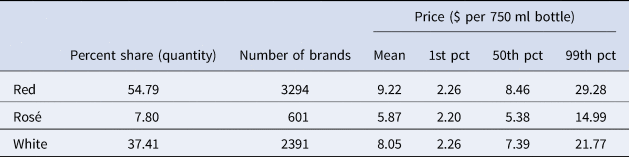
Note: Summary statistics are weighted using Nielsen projection factor.
Source: Nielsen Consumer Panel Data.
Table 2 reports descriptive statistics for red, white, and rosé varietals.Footnote 3 We capture information on 17 red, 13 white, and 8 rosé wine varietals from the data. Additionally, we aggregate any varietal with fewer than 50 observations in the data under the “Other” category. In terms of quantity, Cabernet Sauvignon, Chardonnay, and Zinfandel rosé are the top-selling varietals among red, white, and rosé wines, respectively. In terms of average price, Cabernet Franc, Tempranillo, Pinot Blanc, Viognier, and Pinot Noire rosé fetch a premium relative to other varietals.
Table 2. Sample composition and prices, by varietals
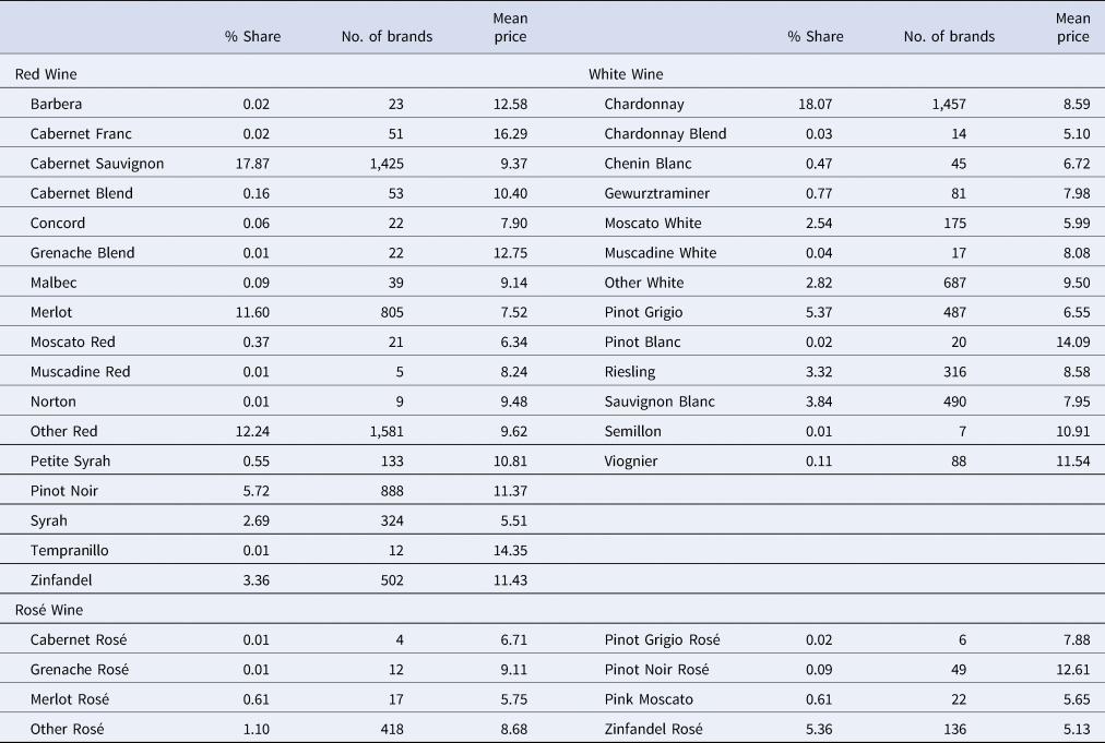
Notes: The % share is computed in volume (quantity) terms, weighted using Nielsen projection factors. Mean price is $/bottle. Cabernet Blend includes Cabernet-Malbec, Cabernet-Merlot, Cabernet-Merlot-Cabernet Franc, Cabernet Syrah. Chardonnay blend includes Chardonnay-Chenin Blanc, Chardonnay-Pinot Noir, Chardonnay-Pinotage, Chardonnay-Semillon, Chardonnay-Viognier. Other White and Other Red include all other entries for which we do not have specific varietal information in the dataset. Other Red also includes red blends.
Source: Nielsen Consumer Panel Data.
We found 3,939 unique brands in the sample over the 13-year period. The average number of brands in a year is about 1,500. The top 50 brands account for about 68% of the total quantity observed in the sample. Table A2 in the Appendix lists the top 50 brands in total quantity in alphabetical order. Based on the information found in the dataset, we can broadly classify geographic information on wine products into three categories: (a) wines with AVA or county names; (b) wines with state appellation of origin; and (c) wines with no specific geographic origin information, referred to in this paper as “U.S. generic.” AVAs are administered by the federal government and provide the most selective tool of geographic differentiation used by U.S. wine producers. Currently, there are 261 approved AVAs in the United States, 143 of which are in California. Under U.S. law, a viticulture area for American wine is “a delimited grape-growing region having distinguishing features, a name and delineated boundary.” AVAs allow vintners and consumers to attribute a given quality, reputation, or other wine characteristics made from grapes grown in an area to its geographic origin.
The Alcohol and Tobacco Trade and Tax Bureau (TTB) is responsible for designating and reviewing all petitions to establish a new or expand an existing AVA. Once the TTB approves an AVA, a producer can include an AVA label if at least 85% of the volume of wine is derived from grapes grown in the named viticulture area.Footnote 4 Augusta, Missouri, was the first wine-growing region approved as an AVA by the TTB in June 1980. Alternatively, producers can use the name of the state or county on their wine bottles if 75% or more of the volume of wine is derived from grapes grown in the named state or county (California and Washington have stricter requirements). In our sample, we find that 23.5% of domestic wine bottles contain AVAs or county appellations, 50% have a state appellation (most of it pertains to the California state appellation), and 26.4% do not claim any particular geographic origin.
Our data capture information on 115 AVAs, but any AVA with fewer than 50 observations is aggregated under the broader region (AVA or county) that it is part of, or is grouped under the “Other AVAs” category. In the end, we are left with information on 81 distinct geographic origins, including 65 AVAs or counties, 15 state appellations, and one U.S. generic group. Table 3 presents the percent share in total quantity, brand presence, and average price (dollars per bottle) for each selected geographic origin.Footnote 5
Table 3. Sample composition and prices, by geographic origin
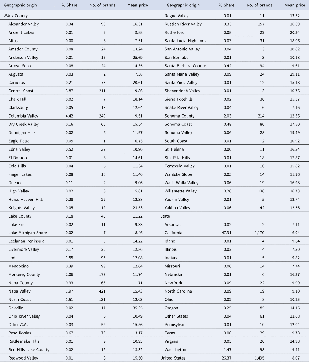
Notes: The % share is computed in volume (quantity) terms and weighted using Nielsen projection factors. Mean price is $/bottle.
Source: Nielsen Consumer Panel Data.
Along with these characteristics, earlier work has shown that vintage and alcohol content are also important attributes of wine prices. However, this information is not available in homescan data. Recent studies that use datasets similar to ours, for other regions, also do not have vintage information (Carew, Florkowski, and Meng, Reference Carew, Florkowski and Meng2017). We use data at the household-trip-UPC level to model the hedonic relationship between wine price and attributes. There are 997,521 observations over the 13-year period from 2007 to 2019. The data includes wine purchase information for over 13,763 unique UPCs over the 13-year period, with an average of about 4,300 distinct UPCs each year. We also include some variables capturing the market characteristics along with wine attributes, which can explain some price variation across markets. Next we will discuss each one.
(1) Channel type
Nielsen consumer panel data also provides information on the channel type from which households purchase wine. Nielsen classifies different channels into 66 mutually exclusive categories. The top nine channel types capture about 96% of the total quantity purchased in the sample. Therefore, we include the top nine channel types and aggregate all other channels into one category. Information on channel type is included in the model to capture variations in price across the retail channel. Table 4 presents the percent share of the top nine channels, the presence of brands, and the average price for a bottle of wine across these channels.
Table 4. Sample composition and price distribution, by retailing channel type
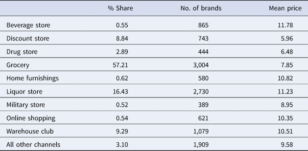
Notes: The % share is computed in volume (quantity) terms and weighted using Nielsen projection factors. Mean price is in $/bottle.
Source: Nielsen Consumer Panel Data.
(2) Retail density
We also capture retail density at the county level to account for price variation across the market. We collect data from County Business Pattern (CBP) at the county level to measure retail density. CBP releases data annually and provides economic data by industry, including the count of establishments and employment level, among other information. CBP follows and provides data from the North American Industry Classification System (NAICS). Under NAICS, retail trade for food and beverage stores is further classified under three sub-categories: (a) grocery stores, sub-classified as supermarkets and other grocery (except convenience stores) or convenience stores; (b) specialty food stores, sub-classified as meat markets, fish and seafood markets, fruit and vegetable markets, or other specialty food stores; and (c) beer, wine, and liquor stores. To count the number of establishments selling wine, we include establishments under categories (a) and (c). We use county-level population and land area to calculate the retail density normalized by spatial area and population. We use American Community Survey (ACS) annual data by the U.S. census to collect county-level population and U.S. census 2010 data to collect the “land area” of a given county. The county-level population from ACS is collected from the IPUMS NHGIS database.Footnote 6 We define “population-adjusted retail density” as the number of establishments per 1,000 residents, and “spatial area adjusted retail density” as the number of establishments per square mile.
(3) State excise tax on wine
The excise tax on wine levied by the state varies a lot across the United States. Along with a three-tier distribution system,Footnote 7 states also impose constraints on the distribution and sales of alcoholic beverages and maintain distribution franchise laws (Santiago and Sykuta, Reference Santiago and Sykuta2016). Young and Bielińska-Kwapisz (Reference Young and Bielińska-Kwapisz2002) show that excise taxes on alcoholic drinks lead to increased alcohol retail prices. Thus, we also control for a state excise tax to capture some variation in wine prices across different states.
We collect wine excise tax data from the Tax Foundation and Federation of Tax Administrators (FTA). States apply varying excise tax rates based on wine type and alcohol content. In 2020, excise taxes differed significantly across states, with the highest in Alaska at $2.50 per gallon, and Pennsylvania, Utah, and Wyoming had no excise tax. These three states with zero excise tax are here referred to as “state control” states because the state government essentially controls all retail wine sales. There is no explicit excise tax on wine in these states, and revenue is generated through various other taxes, fees, price mark-ups, and net profits (FTA). Under the federal code and in some states, sparkling wine has a different excise tax than other wines.Footnote 8 In this study, we consider two categories for excise tax: (a) base excise tax for all wine other than sparkling wine; and (b) excise tax on sparkling wine. In states for which we do not have information about the excise tax on sparkling wine, we consider the base excise tax for sparkling wine. We also account for “state control” states in the model and capture the retail density and excise tax information for only those markets that do not fall under “state control” systems.
IV. The hedonic price model
In a differentiated product market, there are clear modeling advantages to framing consumers’ demand in the characteristics space, following the pioneering work of Gorman (Reference Gorman1956) and Lancaster (Reference Lancaster1966). Traded products are thought of as bundles of characteristics, which is what consumers ultimately care about. There are no markets for the characteristics per se, but the prices of products that are actually bought and sold implicitly define the prices of the characteristics included in them. Rosen's (Reference Rosen1974) seminal paper formalized this insight in the context of a market with a continuum of products and perfect competition. In this setting, the price of a product turns out to be a function of the product's content of characteristics. Consumers are heterogeneous with respect to income and/or preferences for characteristics, and profit-maximizing firms face a convex cost of supplying those characteristics. In Rosen's (Reference Rosen1974) competitive equilibrium, there exists a price function $p( {\vector z})$ such that a good that embeds a vector of characteristics ${\vector z}^i$
 commands a price $p( {\vector z}^i)$
 . This function, termed the hedonic price function, is the envelope of both consumers’ indifference curves (bid functions) and the firms’ iso-profit curves (offer functions). Thus, the hedonic price function represents an equilibrium relation that captures the market's valuation of products’ characteristics that have economic relevance.
It is important to underscore that the hedonic price function describes an equilibrium outcome. Rosen's (Reference Rosen1974) original characterization presumed pure competition, but clearly, an equilibrium price relation linking a product's price to its characteristics also applies to non-competitive markets (Pakes, Reference Pakes2003; Bajari and Benkard, Reference Bajari and Benkard2005; Nesheim, Reference Nesheim2008). As such, the function $p( {\vector z})$ reflects both demand factors pertaining to consumers’ preferences (e.g., consumers’ willingness to pay for individual attributes) as well as supply-side factors (including production costs associated with characteristics and/or market power markups). Disentangling the separate impacts of demand and supply factors is, in general, a difficult matter. The canonical hedonic price function framework envisioned by Rosen (Reference Rosen1974) presumes two empirical stages. The first stage uncovers the structure of the hedonic price function by regressing the prices of traded products against their characteristics. The empirical relation $\hat{p}( {\vector z})$
 thus obtained defines the individual characteristics’ implicit prices ${{\partial \hat{p}( {\vector z}) } / {\partial z_k}}$
 . Such marginal prices naturally reflect the underlying demand and supply conditions, the effects of which could conceivably be uncovered in a second stage, where the estimated characteristics’ implicit prices are the dependent variables.
A large literature articulates the drawbacks of such a two-stage approach. In particular, the identification issues that arise with the second stage are daunting (Brown and Rosen, Reference Brown and Rosen1982; Ekeland, Heckman, and Nesheim, Reference Ekeland, Heckman and Nesheim2002), and standard supply-side shifter instruments do not work (Bartik, Reference Bartik1987; Epple, Reference Epple1987). As a result, empirical analyses of hedonic price functions are often confined to the first stage. Researchers wishing to disentangle demand and supply determinants on the equilibrium prices of differentiated products typically pursue more structural approaches, which are, by construction, amenable to welfare assessments and the study of counterfactual policies (Gandhi and Nevo, Reference Gandhi, Nevo, Ho, Hortacsu and Lizzeri2021).
This paper follows many other studies by restricting attention to the first-stage estimation of the hedonic price function. Because, as articulated in the foregoing, the hedonic price function characterizes equilibrium outcomes, and given that we look at actual retail prices over a large set of market conditions, the determinants of wine prices that we consider include a few variables related to the retail market, in addition to the wines’ own characteristics.
A. Hedonic price function
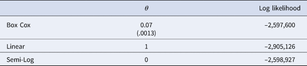
We express the price of wine as a function of the characteristics of interest—wine type, varietals, brand name, and geographic origin—and of market features. Among the latter, we include excise tax, retail density, state distribution rule, the distribution channel of the purchased wine, as well as fixed effects that capture systematic spatial and temporal price effects common across wines. Consistent with much of the previous work on hedonics in wine research reviewed earlier (e.g., Oczkowski, Reference Oczkowski1994; Combris, Lecocq, and Visser, Reference Combris, Lecocq and Visser1997; Carew, Florkowski, and Meng, Reference Carew, Florkowski and Meng2017), we adopt the semi-log parameterization.Footnote 9 That is, the hedonic price equation that is estimated is expressed as:

where p ji is the price of wine product j (at the UPC level) observed at purchase occasion i; and, each purchase occasion pertains to a specific Nielsen-defined major market m = m[i] and occurred in a specific year t = t[i]. On the right-hand-side, ${\vector {\bf z}}_j$ is a vector of wine attributes, which includes wine type, varietal, and geographic origin; ${\vector {\bf x}}_{ji}$
 is a vector of dummies that control for the retail store type in which product j was bought at purchase occasion i; D s is a dummy variable that denotes markets that falls in a state that has total control over wine distribution (here, s = s[i] indicates the state where purchase i took place); T st denotes the state excise tax in the year t; and, R ct is the measure of retail density for county c (where the purchase is made) in year t. Further controls are provided by a rich set of fixed effects: ξ b is the brand fixed effect (where b = b[j] denotes the brand associated with wine product j); ξ m is the market fixed effect; and, ξ q and ξ t are, respectively, the quarter and the year fixed effects. Finally, ɛ ji is the error term, assumed to be identically and independently distributed.
V. Results
Table 5 summarizes the variables included in the hedonic price regression and provides short descriptions. The estimation results are reported in Table 6. Whereas the entire set of estimates will be used for the Shapley value metrics in the next section, here we focus on entries for varietals and geographic origins that have a solid representation in the estimation sample: specifically, at least 0.05% in quantity share (roughly speaking, about 500 bottles over the 13-year period) and at least 10 different brands. The first three columns of results in Table 6 pertain to the hedonic price model as presented in Equation (1), whereas the last three columns are from an expanded model that includes interaction effects between varietals and geographic origin variables.
Table 5. Variables in the hedonic regression
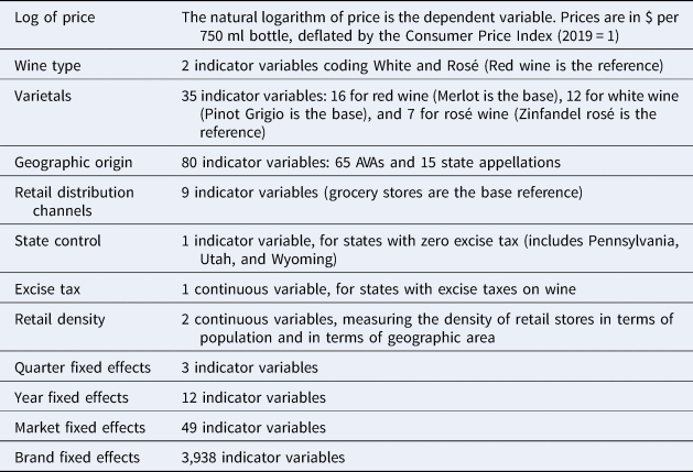
Note: This table provides a summary of the variables included in the hedonic regression.
Table 6. Hedonic price regressions results
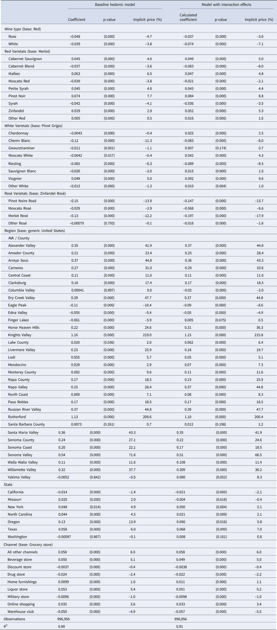
Notes: There are 997,521 observations in total. However, 565 observations that are singletons are dropped when estimating fixed effect regression. The fixed effect regression is estimated using the “REGHDFE” command in Stata. The “calculated coefficients” reported for the “interaction” model pertain to the total effect evaluated at the appropriate conditional mean (see text for more details). The standard error for the interaction model is calculated using the delta method.
In the hedonic price equation, we considered four sets of explanatory variables that relate to wine's intrinsic attributes—wine type, varietals, geographic origin, and brand. In addition, because we are fitting equilibrium retail prices, we also include a set of variables pertaining to retailing conditions, as well as year, quarter, and market fixed effects. The interpretation of these last two sets of variables, of course, differs from the intrinsic wine attributes, but it is important to include them as controls for correct inference about wine's intrinsic attributes.
A. Baseline hedonic model
Because the semilog functional form is used, the coefficients reported in Table 6 are approximately related to the percent premium (or discount) of each attribute relative to the base reference. Specifically, if β k is the estimated coefficient associated with an attribute coded by a dummy indicator variable, the corresponding implicit price, expressed as a percent of the reference wine price, is computed as 100[exp(β k) − 1] (Halvorsen and Palmquist, Reference Halvorsen and Palmquist1980). This percent implicit price is also reported in Table 6. Because of the large number of observations (nearly one million), most estimated coefficients are significantly different from zero at conventional significance levels.
Concerning wine type, we see that red wine (the base reference) carries a premium of about 4%, relative to both white and rosé wine. For varietals, we have a different reference base for each type. Relative to the reference for red wine (Merlot), we find that Cabernet Sauvignon, Malbec, Petite Syrah, Pinot Noir, and Zinfandel all carry a moderate premium, the largest one commanded by Pinot Noir (7.7%). Among white varietals, relative to the chosen reference base (Pinot Grigio), the wines with the largest discounts are Chenin Blanc (–11.3%) and Riesling (–6.3%), whereas Viognier carries a premium of 5%. Chardonnay is essentially equivalent to the Pinot Grigio reference. All rosé varietals included appear to have a discount relative to the base varietal (Zinfandel rosé).
Looking at the geographic origin, it is apparent that most AVA wines carry a considerable price premium relative to the base reference (unspecified U.S. origin). Some selective AVAs like Knight Valley and Rutherford show the largest price premia by far (exceeding 200%). Other well-known AVAs with substantial price premia include Alexander Valley (41.9%), Carneros (31%), Dry Creek Valley (47.7%), Russian River Valley (44.4%), Santa Maria Valley (43.3%), Sonoma Valley (71.6%), and Willamette Valley (37.7%). The price premium associated with Napa labels, by contrast, is somewhat smaller (28.4% for Napa Valley and 18.5% for Napa County). Among the large and well-known AVAs, Columbia Valley is the only one to show a zero price difference relative to the reference (generic U.S. origin).
In interpreting these results, it is important to recall that these are equilibrium price differentials. In addition to consumers’ willingness to pay, they also reflect supply conditions. Furthermore, the estimated price differentials for attributes, such as geographic origin, are conditional on all other variables in the model. Chief among the latter are brands. Indeed, if a firm succeeded in capturing the full set of price-relevant information by means of a brand label, the scope for characteristics to explain price would be void.
As for state appellation, among the large wine-producing states, only Oregon carries a sizeable price premium (13.9%), whereas California and Washington show negligible (and negative) price differentials relative to the reference base. Smaller wine-producing states such as Missouri, New York, North Carolina, and Texas all show moderate and positive price premia relative to the reference (generic U.S. origin).
Table 6 also reports results for the impact of retailing channels, relative to the reference (grocery store). It seems the highest premia are associated with beverage stores and liquor stores (about 5%), and a similar price difference is also associated with the “all other” distribution channel, whereas the largest discount is provided by warehouse clubs.
B. Hedonic model with interaction effects
The wine literature recognizes the existence of possibly important variety-by-location interactions (Alston, Anderson, and Sambucci, Reference Alston, Anderson and Sambucci2015). Therefore, in trying to separate the roles of varietals and geographic origin in affecting prices, it may be desirable to account for such interactions. In addition to the baseline hedonic model discussed in the foregoing, we also estimate a model that includes interaction terms between geographic origin and varietal indicator variables. In other words, we expand the model of Equation (1) to include a set of interaction terms z gz v, where z g denotes geographic origin indicator variables and z v denotes varietal indicator variables. Because we have 38 varietal indicator variables and 81 geographic origin indicator variables, in principle, this adds 3,078 additional explanatory variables to the hedonic price equation. However, many of these interaction effects have zero observations in the sample (e.g., no Barbera in Willamette Valley), such that the net addition of the interaction model amounts to 729 variables.
The results for the interaction model are reported in the last three columns of Table 6. The coefficients and the implicit prices reported there pertain to the total effect evaluated at the relevant conditional means. For example, if the kth attribute of interest is the AVA “Carneros,” then the coefficient reported for the interaction model is $\beta _k + \sum\nolimits_v {\delta _{kv}E[ { {z_v} \vert AVA = k} ] }$ , where, as before, β k is the coefficient of the stand-alone Carneros indicator variable, and δ kv denotes the parameters of the interaction variables between the Carneros region and varietal indicators. The standard error for this total coefficient, and the associated p-value, are calculated using the delta method. Given such a calculation of the interaction total coefficient, the implicit price, expressed as a percent, is then computed in the same fashion as noted earlier.
From Table 6, we see that the model with interaction effects entails a large price discount for white wine relative to the reference of red wine (–7.1%). As for the implicit prices of varietals and geographic origin attributes, the results of the interaction model are quite similar to those of the baseline model. For example, the correlation coefficient between the implicit prices of varietals across the two models is 0.924. Some minor differences, resulting from introducing interaction effects, include a larger discount for Cabernet blends and Riesling, and a larger premium for Zinfandel and Chardonnay. As for the implicit prices for geographic origin attributes, they are extremely close: the correlation coefficient between the implicit prices of the baseline and the interaction models is 0.995. Among the few notable differences that we observe is that the model with interaction effects predicts larger premia for Napa wines (e.g., the Napa Valley premium increases from 28.4 to 44.8%).
We do not necessarily believe that the interaction model is “better” for the purposes of the research question in this paper. At a minimum, however, this provides a robustness check on the conclusions we derive vis-à-vis the implicit prices of varietals and geographic origin. The conclusion from the results in Table 6 is that the two models are quite consistent, and both indicate moderate impacts of varietals and larger impacts of geographic origin on estimated implicit prices. We note, again, that these are ceteris paribus effects, after accounting for other likely sources of product differentiation, including extensive controls for wine brands.
C. Relative importance of attributes: Shapely values
Having established that the explanatory variables included in the hedonic price equations have non-negligible price impacts, as evidenced by the computed implicit prices, here we investigate the relative importance of the various attributes in the determination of equilibrium wine prices. In particular, just how important is the geographic origin information provided by AVA, county, and state appellations? How does geography as a marketing tool compare with, say, the role of variety information? To answer these questions, we apply a technique that assesses the relative importance (influence) that independent variables contribute to a model's predictive abilities. The approach is inspired by the Shapley value concept from cooperative game theory, which is finding widespread interest in modern machine learning methods (Lundberg and Lee, Reference Lundberg, Lee, von Luxburg and Guyon2017).
Our application of the Shapley value approach follows the original development provided by Lipovetsky and Conklin (Reference Lipovetsky and Conklin2001) to evaluate the relative importance of individual variables in a linear model's prediction. The main criterion to assess the latter is the regression fit as measured by the R 2 statistics. The key is a decomposition of this metric that provides attribution shares to each right-hand-side variable. To see how this objective is related to one of the more celebrated concepts in game theory, it is helpful to recall the basics of the Shapley value (see Roth (Reference Roth and Roth1988) for a lucid discussion). The setting is one where any subset of the set N ≡ {1, 2, …, n} of players can create value by cooperating. The latter is measured by the characteristic function v that maps any coalition of a subset S ⊆ N of players to a real number v(S) that summarizes the overall value of the game. How much does each individual participant contribute to the coalition? One could start by looking at the marginal contribution of player i when participating in a coalition S, that is, Δi = v(S) − v(S − {i}). The problem, of course, is that this marginal value depends on the specific subset S one considers. Shapley (Reference Shapley, Kuhn and Tucker1953) provides an axiomatic formulation where, nonetheless, a unique “Shapley value” ϕ i(v) for each player can be obtained such that the value of the grand coalition v(N) is fully distributed, that is, $\sum\nolimits_{i\in N} {\phi _i( v) = v( N) }$ .
.
The Shapley value is, essentially, the average over all possible marginal contributions Δi (i.e., the marginal contribution of player i evaluated with respect to all possible coalitions it can be part of). That is, the Shapley value can be expressed as
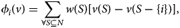
where the weights associated with each coalition are w(S) = (m − 1)!(n − m)!/n!, with m denoting the size of coalition S (which, as noted earlier, n is the number of all possible players, that is, the size of the grand coalition).Footnote 10
The parallel with the problem at hand is apparent as we now conceive of individual explanatory variables as “players” that cooperate in a regression, where the value of their cooperation is measured by the quality of the model's fit. As a metric for the latter, Lipovetsky and Conklin (Reference Lipovetsky and Conklin2001) focus on the traditional R 2 statistics. The beauty and apparent notional simplicity of the Shapley value in Equation (2) hides challenging computational issues, however. With a set of n players, one needs to evaluate the coalition value v(⋅) for (2n − 1) possible coalitions—a magnitude that increases exponentially with the number of players n. In our context, for a regression involving n explanatory variables, to impute a Shapley value contribution to each individual regressor, one needs to run (2n − 1) regressions, something that is challenging for even moderate regression sizes, and clearly not feasible in our context.Footnote 11
The economic question of interest, however, does not concern individual regressors but rather the value contribution of sets of regressors. That is, we are not so much interested in how the information concerning one AVA adds much to explaining wine equilibrium prices; we care more about understanding whether the set of all AVAs, collectively, adds in a meaningful way to explaining equilibrium wine prices. Thus, to assess such broad features of the empirical hedonic price model, we implement the Shapley value decomposition of the model's R 2 for groups of variables rather than for individual regressors. For Shapely value imputation, we specifically consider six groups, which include: (i) wine type, (ii) varietals, (iii) geographic origin, (iv) market characteristics (e.g., retail channel type), (v) brand fixed effects, and (vi) year, season, and region fixed effects.
Given the current specification, we have 63 “coalitions” of explanatory variables. Let subscripts a, b, c, d, e, and f denote each of these six groups of regressors. Then the grand coalition, including all explanatory variables, will have a model fit that is denoted $R_{abcdef}^2$ . Omitting all variables except variety-related variables, on the other hand, would lead to a model with fit denotes $R_b^2$
 , while omitting varietals but including everything else yields a model fit $R_{acdef}^2$
 . Hence, the marginal value of feature b, relative to the empty set, is simply R b (recall that $v( \emptyset ) = 0$
 ). The marginal value of feature b when all other features are present, on the other hand, is $R_{abcdef}^2 -R_{acdef}^2$
 . In this fashion, we can construct the marginal value of feature b relative to all possible coalitions, such that we can implement Equation (2) and construct the Shapley value for this feature. And this can be done for all of the six features of interest that we have identified.Footnote 12 By construction, these Shapley values will satisfy $\phi _a + \phi _b + \phi _c + \phi _d + \phi _e + \phi _f = R_{abcdef}^2$
 .
.
The results for the Shapley value decomposition are reported in Table 7. Using the R 2 metric of the baseline model, we find that, for equilibrium prices, brand-fixed effects are the most important determinants, accounting for 72%. Geographic origin is next, accounting for 10.7%, whereas varietals account for 6.2% and wine type for 1.4%. The two sets of control variables that we include in the hedonic price equation (e.g., retail distribution channels and other fixed effects) account for about 10%.
Table 7. Shapley values
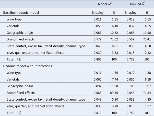
Notes: This table reports the Shapley value metrics for the relative importance of sets of variables.
The large relative importance that Shapley values associate with brands vindicates the presumption, noted in the introduction, that repeat purchases are important in markets with experience goods, such that the provision of quality can be supported by credible branding strategies. Notwithstanding the role played by firms’ individual brands in the wine market, however, it is apparent that “collective” branding messages conveyed by geographic origin are quite important. This is an accepted fact for Old World wine marketing (e.g., Castriota, Reference Castriota2020), but the foregoing results imply that, even for New World wines, credible certification of geographic origin matters. In fact, we find that the relative importance of geographic origin clearly exceeds the role played by varietals. This is consistent with other work showing that region of origin is usually more significant as a determinant of price than grape variety (e.g., Steiner (Reference Steiner2004) for Australia, and Costanigro, McCluskey and Mittelhammer (Reference Costanigro, McCluskey and Mittelhammer2007) for North America).
The decomposition in the first two columns of Table 7 pertains to the R 2 for Equation (1), which fits the log of price. From an economic point of view, of course, the implied fitted price from the estimated equation is what matters most. From the estimated semilog model, with log fitted values $\hat{y}_i\equiv \ln p_i-\hat{\varepsilon }_i$ , with a normal distribution the implied fitted price is $\hat{p}_i = \exp ( \hat{y}_i) \ast \exp ( {{{{\hat{\sigma }}^2} / 2}} )$
 , where $\hat{\sigma }^2$
 is the estimated variance of the regression error. Implied price residuals are thus $\hat{u}_i\equiv p_i-\hat{p}_i$
 , and the implied coefficient of determination for predicting prices themselves is $\tilde{R}^2 = 1-{{\sum\nolimits_i {\hat{u}_i^2 } } / {\sum\nolimits_i {{( {p_i-\bar{p}} ) }^2} }}$
 . The Shapley value decomposition based on$\tilde{R}^2$
 is also reported for the baseline model in Table 7. The results are similar to those based on the semilog R 2, and in fact, further emphasize the main take-home points: brands are the most important determinants, geographic origin is next, and geographic origin matters quite a bit more than varietals.
The second part of Table 7 reports the results for the model with interaction variables. The results are broadly consistent with those of the baseline model. The main impact of adding interaction effects, relative to the baseline, is to moderate slightly the impact of firms branding, which decrease from 75.4 to 71.5%, and to increase the role of geographic origin, which increases from 12 to 14% (for the metric based on $\tilde{R}^2$ ).
).
VI. Conclusion
In this paper, we analyze the determinants of retail wine prices in the U.S. market for wine consumed at home, with the objective of characterizing the main dimensions of product differentiation. We focus on U.S.-produced wines, sold in standard 750 ml bottles, and rely on an extensive dataset from Nielsen homescan data, obtained from a large and representative sample of household purchases from 2007 to 2019. Data extracted from products’ UPC label description permits us to construct a large set of controls, including individual products’ brands, wine varietal, and geographic origin. Our hedonic price model also includes extensive controls for other local factors likely affecting retail prices.
Our empirical findings suggest that, after accounting for firms’ brands, wine types, varietals, and other control variables, information about the geographic origin of U.S. wines carries considerable explanatory power. In particular, AVA labels are associated with significant price premia, relative to an undefined U.S. origin, over and above that secured by the effects of firms’ brands. Our paper also proposes the use of an attractive metric to characterize the overall importance of a set of determinants of wine price, a measure based on the Shapley value from cooperative game theory. Using this metric, we find that over 70% of U.S. retail wine prices are accounted for by individual wines’ own brands, a finding consistent with the basic economics of markets for experience goods and the role of reputation. We also find that geographic origin is the next most important predictor of wine prices, again even after accounting for the effects of brands. In particular, Shapley values suggest that the contribution of geographic origin is considerably greater (about twice as large) than that of varietals.
These findings have interesting implications for wine producers’ marketing strategies and for policy. Whereas it is accepted that geographic origin information is essential for marketing Old World wines, especially wines from the European Union, conventional wisdom holds that such factors matter less for New World wines. Indeed, one of the marketing tools emphasized by New World wineries has been the use of varietals. Notwithstanding that, however, starting in the 1980s, the U.S. industry developed a standardized system of geographic origin denominations, centered on AVAs, that provides collective labeling options similar to those widely used in Europe. Our results vindicate this evolution and suggest that, indeed, AVA labeling is an important element of product differentiation, highly complementary to firms’ marketing strategies captured by their own brands.
Acknowledgments
The authors thank the editor, Karl Storchmann, and an anonymous reviewer for their constructive comments.
Researcher(s)' own analyses calculated (or derived) based in part on data from Nielsen Consumer LLC and marketing databases provided through the NielsenIQ Datasets at the Kilts Center for Marketing Data Center at The University of Chicago Booth School of Business. The conclusions drawn from the NielsenIQ data are those of the researcher(s) and do not reflect the views of NielsenIQ. NielsenIQ is not responsible for, had no role in, and was not involved in analyzing and preparing the results reported herein.
The author(s) declare that they have no competing interests.
Appendix A
Table A1. Wine products in the Nielsen consumer panel data
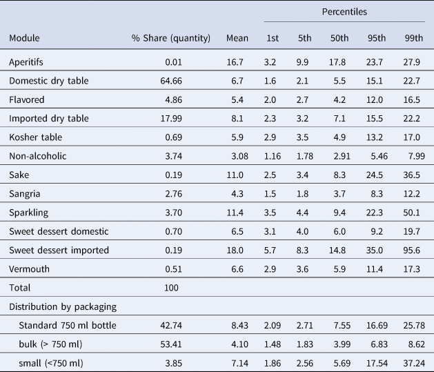
Table A2. List of top 50 brands in terms of market share (names if alphabetical order)
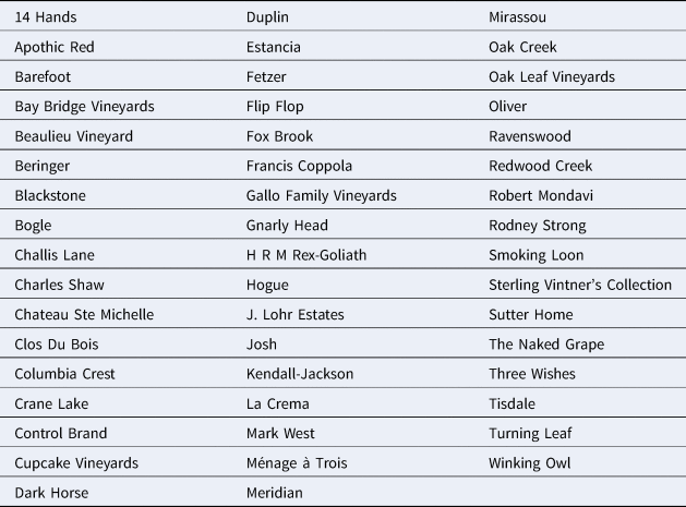
Table A3. Box Cox regression
Appendix B: Extracting text data from UPC description
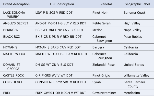
We extract the wine attribute information, such as type, varietal, and geographic origin, from the UPC description in the Nielsen data. Table B1 presents some examples of UPC and brand descriptions from the Nielsen data. Varietal and geographic label columns show information extracted from UPC descriptions. We used regular expressions in Stata to code this information extraction. For most UPC descriptions, the first word is generally the band name. Brand information is also provided by Nielsen as a separate variable. The remaining letters stand for country name, region, and varietal. For instance, CHRD is Chardonnay, P-GR is Pinot Grigio, MLBC is Malbec, MRLT is Merlot, WT is White, DDT is Domestic Dry Table, BLS is Blush, etc. We did find some redundancies, where more than one abbreviation for one word could be used (e.g., Moscato could be MSC, MSCT, or MUSCATO). We did our best to cross-check such entries. Further, to ensure that these abbreviations mean what we take them to mean, we cross-checked our inferences by matching brand names and UPC descriptions with information at the site www.wine-searcher.com, which has a comprehensive list of wines with brand names, grape blends, and geographic origins.
Table B1. Examples of UPC description from Nielsen data
Wine brand names also come with small variations, and Nielsen assigns new codes to the brands even with the slightest variation in brand description. In this study, we are treating different variants of a brand as one brand. For instance, Francis Coppola dmnd cltn, Francis Coppola diamond cllctn, Francis coppola presents, Francis Coppola Director's cut are considered as one brand Francis Coppola. As another example, brand Robert Mondavi includes: Robert Mondavi, Woodbridge Rbrt Mndv, Robert Mondavi Private Selection, La Famiglia di Robert Mondavi, Woodbridge Rbrt Mndv Slt Vy Sr, and Woodbridge by Robert Mondavi.


 Open access