


1. Introduction
The goal of multi-objective reinforcement learning (MORL) is to expand the generality of reinforcement learning (RL) methods to enable them to work for problems with multiple conflicting objectives (Roijers et al., Reference Roijers, Vamplew, Whiteson and Dazeley2013; Hayes et al., Reference Hayes, Rădulescu, Bargiacchi, Källström, Macfarlane, Reymond, Verstraeten, Zintgraf, Dazeley, Heintz, Howley, Irissappane, Mannion, Nowé, Ramos, Restelli, Vamplew and Roijers2022b). Traditional RL normally assumes that the environment is a Markov decision process (MDP) in which the agent will receive a scalar reward after performing each action, and the goal is to learn a policy that maximises a single long-term return based on those rewards (Sutton & Barto, Reference Sutton and Barto2018). In contrast, MORL works with MOMDPs, where the reward values are vectors, with each element in the vector corresponding to a different objective. Using vector rewards overcomes the limitations of scalar rewards (Vamplew et al., Reference Vamplew, Smith, Källström, Ramos, Rădulescu, Roijers, Hayes, Heintz, Mannion and Libin2022b) but also creates a number of new algorithmic challenges.
One of the most common approaches used so far in the MORL literature is to extend standard scalar RL algorithms such as Q-learning or Deep Q-Networks to handle vector rewards. We will cover the details of how this is achieved in Section 2.2. While this method has been successfully applied, it has also been demonstrated to have some significant shortcomings, particularly in the context of environments with stochastic rewards and/or state transitions (Vamplew et al., Reference Vamplew, Foale and Dazeley2022a).
This paper provides a more detailed examination of the issues identified by Vamplew et al. (Reference Vamplew, Foale and Dazeley2022a). We explore various methods by which the issues caused by the local decision-making aspect of Q-learning might be solved or ameliorated, including changes in reward design, as well as algorithm modifications. In addition we examine the extent to which the noisy Q-value estimates issue is a key factor impeding the ability of value-based MORL methods to converge to optimal solutions in stochastic environments.
Section 2 provides the required background, giving a general introduction to MORL and MOMDPs, as well as more specific detail on the issues faced by value-based MORL algorithms in environments with stochastic state dynamics. Section 3 provides an overview of the experimental methodology, including the Space Traders MOMDP which will be used as a benchmark. The following four sections report and discuss experimental results from four different approaches (baseline multi-objective Q-learning, reward engineering, an extension of MO Q-learning to incorporate global statistics, and MO Q-learning using policy options). The paper concludes in Section 8 with an overview of the findings, and suggestions for future work to address the task of learning optimal policies for stochastic MOMDPs.
2. Background
2.1 Multi-objective reinforcement learning
The basic multi-objective sequential decision problem can be formalised as a multi-objective Markov decision process (MOMDP). It is represented by the tuple
 $\langle S, A, T, \mu, \gamma, \textbf{R} \rangle$
where:
$\langle S, A, T, \mu, \gamma, \textbf{R} \rangle$
where:
-
• S is a finite set of states
-
• A is a finite set of actions
-
•
 $T\,: \,S\times A\times S\rightarrow[0,1]$
is a state transition function
$T\,: \,S\times A\times S\rightarrow[0,1]$
is a state transition function -
•
$\mu\,:\, S\rightarrow[0,1]$
is a probability distribution over initial states -
•
$\gamma\in[0, 1)$
is a discount factor -
•
$\textbf{R}$
$:\, S\times A\times S\rightarrow R^d$
is a vector-valued reward function which defines the immediate reward for each of the
$d\geq2$
objectives.


So the main difference between a single-objective MDP and a MOMDP is the vector-valued reward function
 $\textbf{R}$
, which specifies a numeric reward for each of the considered objectives. The length of the reward vector is equal to the number of objectives. The generalisation of RL to include vector rewards introduces a number of additional issues. Here we will focus on those which are of direct relevance to this study; for a broader overview of MORL we recommend (Roijers et al., Reference Roijers, Vamplew, Whiteson and Dazeley2013; Hayes et al., Reference Hayes, Rădulescu, Bargiacchi, Källström, Macfarlane, Reymond, Verstraeten, Zintgraf, Dazeley, Heintz, Howley, Irissappane, Mannion, Nowé, Ramos, Restelli, Vamplew and Roijers2022b).
$\textbf{R}$
, which specifies a numeric reward for each of the considered objectives. The length of the reward vector is equal to the number of objectives. The generalisation of RL to include vector rewards introduces a number of additional issues. Here we will focus on those which are of direct relevance to this study; for a broader overview of MORL we recommend (Roijers et al., Reference Roijers, Vamplew, Whiteson and Dazeley2013; Hayes et al., Reference Hayes, Rădulescu, Bargiacchi, Källström, Macfarlane, Reymond, Verstraeten, Zintgraf, Dazeley, Heintz, Howley, Irissappane, Mannion, Nowé, Ramos, Restelli, Vamplew and Roijers2022b).
2.1.1 Action selection and scalarisation
The most obvious issue is that the optimal policy is less clear because there may be multiple optimal policies (in terms of Pareto optimality). Therefore, MORL requires some approach for ordering those vector values.
There has been a trend in recent literature to adopt a utility-based approach as proposed by Roijers et al. (Reference Roijers, Vamplew, Whiteson and Dazeley2013). This approach utilises domain knowledge to define a utility function which captures the preferences of the user. In value-based MORL, the utility (aka scalarisation) function is used to determine an ordering of the Q-values for the actions available at each state, in order to determine the action which is optimal with respect to the user’s utility. These functions can be broadly divided into two categories, which are linear and monotonically increasing nonlinear functions.
Linear scalarisation is straightforward to implement, as it converts the MOMDP to an equivalent MDP (Roijers et al., Reference Roijers, Vamplew, Whiteson and Dazeley2013). However, it also suffers from a fundamental disadvantage that it is incapable of finding deterministic policies with expected returns lying in concave regions of the Pareto front (Vamplew et al., Reference Vamplew, Yearwood, Dazeley and Berry2008)Footnote 1 . Also in some situations, a linear scalarisation function is not sufficient to handle all types of user preferences. For example, MORL approaches to fairness in multi-user systems use nonlinear functions such as the Nash Social Welfare function or the Generalised Gini Index (Siddique et al., Reference Siddique, Weng and Zimmer2020; Fan et al., Reference Fan, Peng, Tian and Fain2022).
Therefore, monotonically increasing (nonlinear) scalarisation functions have been introduced (e.g. Van Moffaert et al., Reference Van Moffaert, Drugan and Nowé2013). These adhere to the constraint that if a policy increases for one or more of the objectives without decreasing any of the other objectives, then the scalarised value also increases (Hayes et al., Reference Hayes, Rădulescu, Bargiacchi, Källström, Macfarlane, Reymond, Verstraeten, Zintgraf, Dazeley, Heintz, Howley, Irissappane, Mannion, Nowé, Ramos, Restelli, Vamplew and Roijers2022b). One notable example is the thresholded lexicographic ordering (TLO) method which allows agent to select actions prioritised in one objective and meet specified thresholds on the remaining objectives (Gábor et al., Reference Gábor, Kalmár and Szepesvári1998; Issabekov & Vamplew, Reference Issabekov, Vamplew, Thielscher and Zhang2012).
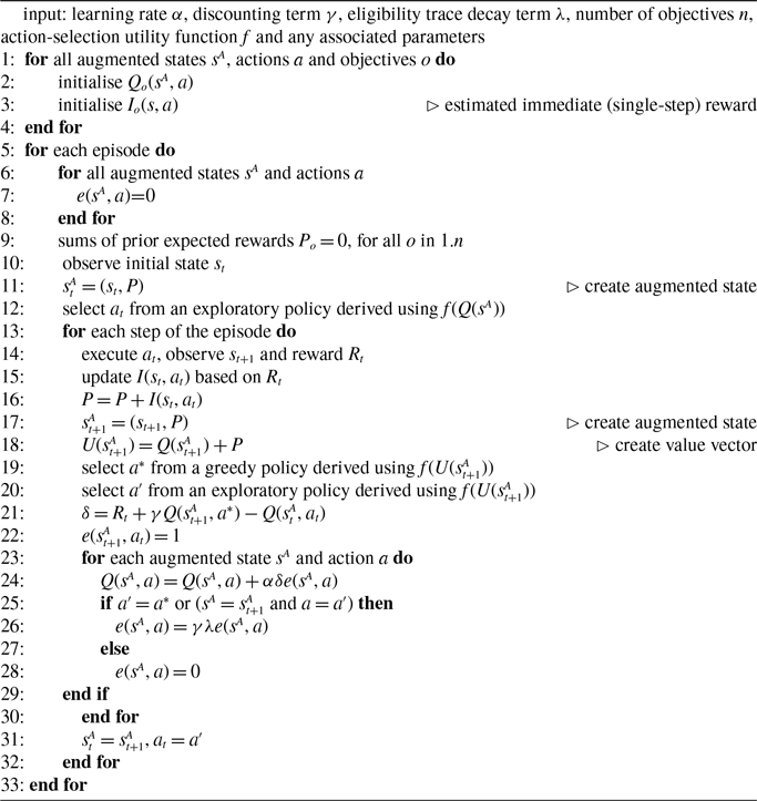
Under non-linear functions (such as TLO) the rewards are no longer additive which violates the usage of the Bellman equation for value-based methods (Roijers et al., Reference Roijers, Vamplew, Whiteson and Dazeley2013). To address this, for value-based MORL both action selection and Q-values must be conditioned on the current state as well as a summary of the history of prior rewards (see Algorithm 1 —lines 11 and 17 create an augmented state via a concatenation of the environmental state and the history of prior rewards, and Q-values and action selection are based off this augmented state).
2.1.2 Single-policy versus multi-policy methods
In single-objective RL the aim is to find a single, optimal policy. In contrast for MORL, an algorithm may need to find a single or multiple policies depending on whether or not the user is able to provide the utility function prior to the learning or planning phase. For example, if the user already knows in advance their desired trade-off between each objective, then the utility function is known in advance and fixed. Therefore there is no need to learn multiple policies as the agent can simply find the optimal policy which maximises that utility. On the other hand, if the utility function cannot be designed before the training or the preferences could change over time, then the agent has to return a coverage set of all potentially optimal policies. The user will then select from this set to determine which policy will be used in a particular episode.
If we consider the scenario of planning a trip as an example, the traveller may or may not know the exact preferences about getting to the destination in terms of when to get there and how much the traveller is willing to spend on this journey. So in this case, the algorithm needs to learn all non-dominated policies. However, if the traveller has a preference about how long they can take to arrive at their destination or there is a certain budget associated with this trip, then a single policy will be enough to satisfy their preferences.
2.1.3 Scalarised expected returns versus expected scalarised returns
According to Roijers et al. (Reference Roijers, Vamplew, Whiteson and Dazeley2013), there are two distinct optimisation criteria compared with just a single possible criteria in conventional RLFootnote
2
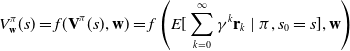
. The first one is expected scalarised return (ESR). In this approach, the agent aims to maximise the expected value which is first scalarised by the utility function, as shown below (Equation 1) where w is the parameter vector for utility function f,
 $r_k$
is the vector reward on time-step k, and
$r_k$
is the vector reward on time-step k, and
 $\gamma$
is the discounting factor
$\gamma$
is the discounting factor
 \begin{equation}V^\pi_\textbf{w}(s) = E[f\left( \sum^\infty_{k=0} \gamma^k \mathbf{r}_k,\textbf{w}\right)\ | \ \pi, s_0 = s)\end{equation}
ESR is the appropriate criteria for problems where the aim is to maximise the expected outcome within each individual episode. A good example is searching for a treatment plan for a patient, where there is a trade-off between cure and negative side effect. Each patient would only care about their own individual outcome instead of the overall average.
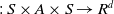
The second criteria is scalarised expected return (SER), which estimates the expected rewards per episode and then maximises the scalarised expected return, as shown in (Equation 2)
 \begin{equation}V^\pi_\textbf{w}(s) = f( \textbf{V}^\pi(s), \textbf{w}) = f\left(E[\sum^\infty_{k=0} \gamma^k \mathbf{r}_k \ | \ \pi, s_0 = s], \textbf{w}\right)\end{equation}
So SER formulation is used for achieving the optimal utility considered over multiple executions. Continuing with the travel example, the employee wants to cut down on the amount of time spent travelling to work each day. Travelling by car would be the good option on average, although there may be rare days on which it is considerably slower due to an accident.
2.2 Multi-objective Q-learning and stochastic environments
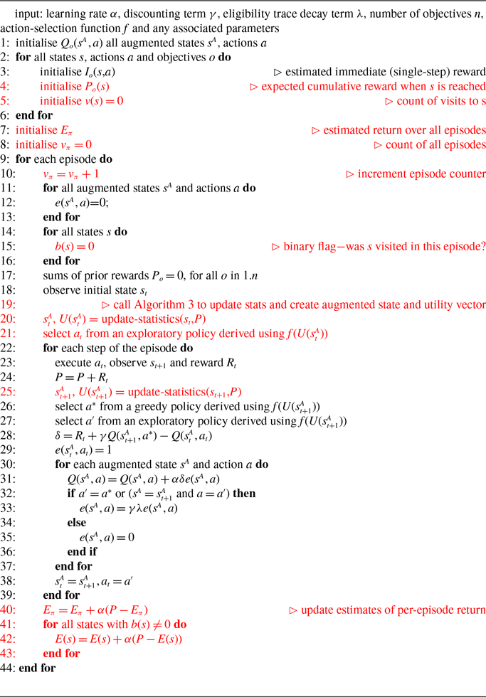
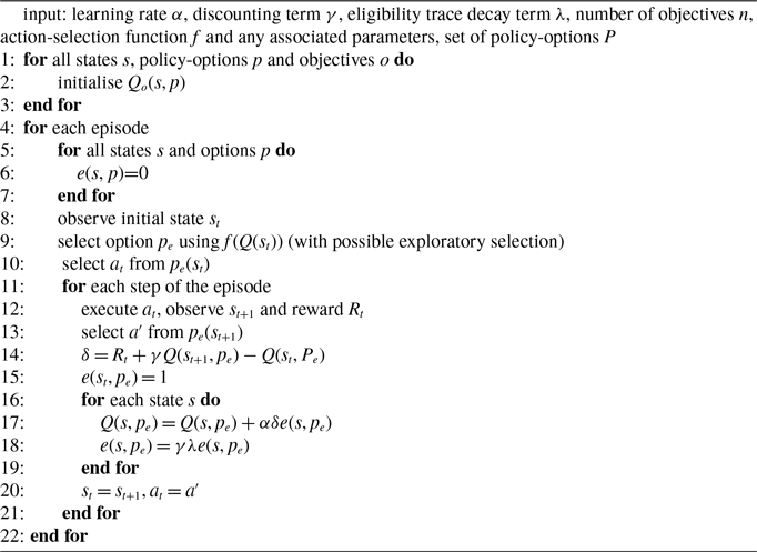
In contrast to much of the prior work on MORL which has used deterministic environments, Vamplew et al. (Reference Vamplew, Foale and Dazeley2022a) examined the behaviour of multi-objective Q-learning in stochastic environments. They demonstrated that in order to find the SER-optimal policy for problems with stochastic rewards and a non-linear utility function, the MOQ-learning algorithm needs action selection and Q-values to be conditioned on the summed expected rewards in the current episode, rather than the summed actual rewards (see Lines 15–18 in Algorithm 1).
Algorithm 1 Multi-objective Q(
 $\lambda$
) using accumulated expected reward as an approach to finding deterministic policies for the SER context (Vamplew et al., Reference Vamplew, Foale and Dazeley2022a)
$\lambda$
) using accumulated expected reward as an approach to finding deterministic policies for the SER context (Vamplew et al., Reference Vamplew, Foale and Dazeley2022a)
2.2.1 SER optimality and local decision-making
Vamplew et al. (Reference Vamplew, Foale and Dazeley2022a) also identified that existing value-based model-free MORL methods may fail to find the SER optimal policy in environments with stochastic state transitions. Under this type of environment, following the same policy may result in different trajectories and rewards in each episode. Since the scalarised expected reward (SER) criteria aims to achieve the optimal utility over multiple executions, the overall policy in order to meet that constraint depends on the probability with which each trajectory is encountered. Therefore, determining the correct action to select at each possible trajectory requires the agent to also consider the returns received in every other trajectory in combination with the probability of that trajectory having been followed (Bryce et al., Reference Bryce, Cushing and Kambhampati2007).
This requirement is incompatible with standard value-based model-free methods like Q-learning, where it is assumed that the best action can be fully determined from the local information available to the agent at the current state. Augmenting that state information with the sum of expected rewards as in Algorithm 1 is insufficient as this still only provides information about the trajectory which has been followed in this episode, rather than all possible trajectories that agent might experience under this same policy.
A recent paper by Vincent (Reference Vincent2024) proposes a model-free, value-based MORL algorithm called K-learning which can, on most executions, successfully learn the optimal SER policy on the environments from Vamplew et al. (Reference Vamplew, Foale and Dazeley2022a). This is achieved by conditioning the Q-values and the newly introduced K-values (and hence the resulting policy) on the entire trajectory rather than just the current state. As such, this approach suffers from scaling issues, as a tabular implementation of K-learning has memory requirements that are exponential with respect to the number of states. One of the aims of this paper is to examine whether SER-optimality can be reliably achieved by value-based algorithms which are more suitable for large environments.
2.2.2 Noisy estimates
A second issue, identified by both Vamplew et al. (2021) and Vamplew et al. (Reference Vamplew, Foale and Dazeley2022a), is the problem of noisy Q-value estimates. The current policy of the agent is determined by the Q-values, which estimate the value of each action in the current state. Small errors in these estimates may lead to the selection of an alternative action.
Noisy estimates are not unique to multi-objective RL. It is well-known that value-based RL algorithms may produce estimates which deviate from the true values, with Q-learning in particular being prone to over-estimation (Van Hasselt et al., Reference Van Hasselt, Doron, Strub, Hessel, Sonnerat and Modayil2018). However, MORL using non-linear scalarisation is particularly sensitive to any errors in Q-values. Consider a situation in scalar RL where only two actions exist (
 $a_1$
and
$a_1$
and
 $a_2$
) and
$a_2$
) and
 $a_1$
is optimal, that is for the true values of each action,
$a_1$
is optimal, that is for the true values of each action,
 $Q(a_1) \gt Q(a_2)$
. If the addition of a small amount of estimation noise is sufficient for the agent to instead prefer
$Q(a_1) \gt Q(a_2)$
. If the addition of a small amount of estimation noise is sufficient for the agent to instead prefer
 $a_2$
(i.e. if
$a_2$
(i.e. if
 $Q(a_1) \lt Q(a_2)+\epsilon$
), then this implies that the loss of utility from this incorrect decision can be no larger than
$Q(a_1) \lt Q(a_2)+\epsilon$
), then this implies that the loss of utility from this incorrect decision can be no larger than
 $\epsilon$
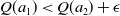
. A similar argument holds for the multi-objective case with linear scalarisation. However, in the context of MORL with non-linear utility, this impact can be much larger as two actions with very different reward vectors may have similar scalarised values. This is particularly true for highly non-linear functions like TLO. Here a small change in the estimated value of the thresholded objective for an action can lead to it incorrectly being regarded as now satisfying the threshold (or vice-versa). Hence small amounts of noise may have a large impact on the actual reward vector received. Consider an example with two objectives where
$\epsilon$
. A similar argument holds for the multi-objective case with linear scalarisation. However, in the context of MORL with non-linear utility, this impact can be much larger as two actions with very different reward vectors may have similar scalarised values. This is particularly true for highly non-linear functions like TLO. Here a small change in the estimated value of the thresholded objective for an action can lead to it incorrectly being regarded as now satisfying the threshold (or vice-versa). Hence small amounts of noise may have a large impact on the actual reward vector received. Consider an example with two objectives where
 $Q(a_1) = (10, 5)$
,
$Q(a_1) = (10, 5)$
,
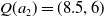 $Q(a_2) = (8.5,6)$
and the user’s utility function based on TLO is defined as
$Q(a_2) = (8.5,6)$
and the user’s utility function based on TLO is defined as
 $f(\vec{v}) = v_2 $
if
$f(\vec{v}) = v_2 $
if
 $ v_1\gt0.88 $
and
$ v_1\gt0.88 $
and
 $v_2-100$
otherwise. Adding a small amount of noise
$v_2-100$
otherwise. Adding a small amount of noise
 $(0.5, 0) $
to
$(0.5, 0) $
to
 $Q(a_2)$
will cause the agent to perceive this action to have a utility of 6 and hence prefer it to
$Q(a_2)$
will cause the agent to perceive this action to have a utility of 6 and hence prefer it to
 $a_1$
. But the actual utility of
$a_1$
. But the actual utility of
 $a_2$
is -94, which is substantially lower than the true utility of
$a_2$
is -94, which is substantially lower than the true utility of
 $a_1$
which is 5. This demonstrates that for a non-linear definition of utility, the relationship between the magnitude of noise in Q-value estimates and the regret from errors induced by that noise is itself non-linear, and therefore, small errors in estimates may give rise to arbitrarily large losses in user utility.
$a_1$
which is 5. This demonstrates that for a non-linear definition of utility, the relationship between the magnitude of noise in Q-value estimates and the regret from errors induced by that noise is itself non-linear, and therefore, small errors in estimates may give rise to arbitrarily large losses in user utility.
As well as having an immediate impact on the utility of the user, noisy estimates may also negatively impact on the actual learning process of a MORL agent. Vamplew et al. (Reference Vamplew, Foale and Dazeley2024) identified a phenomenon which they label value interference, that can arise when an MORL agent attempts to learn Q-values which are vectors. When a particular action (s,a) can lead to multiple different vector returns, the agent will tend to learn a value of Q(s,a) which is a mean of those future returns, weighted by the frequency with which these are experienced. For non-linear f, the utility of that weighted mean may differ considerably from the utility of the actual future returns, and this may interfere with the agent’s convergence to the optimal policy. Vamplew et al. (Reference Vamplew, Foale and Dazeley2024) demonstrate value interference arising from stochasticity, either in the environment itself or in the behaviour of the agent. Noisy estimates can also produce conditions under which value interference can occur. If noisy estimates lead to the agent’s choice of optimal action changing frequently (as is evident in the empirical results later in this paper, such as in Figure 2), the Q-values at previous states will transition from those of the previously greedy action to the new greedy action. If those actions have substantially different vector values, this may cause value interference and hinder the agent’s learning. Again, value interference arises only in the context of vector Q-values and non-linear scalarisation, so this particular impact of noisy estimation is specific to learning under those conditions.
The problem of noisy estimates is not specific to stochastic environments. However, it will be more evident in this context as the variation in future returns due to the stochasticity will in itself result in greater variation in the Q-value estimates.
3. Experimental methodology
The previous section identified two factors that might prevent value-based MORL algorithms from learning SER-optimal policies in stochastic environments—local decision-making and noisy estimates. The main aim of this paper is to examine the importance of these factors, and to empirically explore possible approaches for addressing these issues, while remaining within the overall model-free value-based MORL framework. We provide here an overview of the aspects of the experimental methodology which were common across all experiments, while later sections will provide details of the individual approaches and any specific experimental modifications required during their evaluation.
3.1 Approaches tested
The experiments evaluate four MORL methods, including a baseline method.
-
• Baseline approach—This is basic MOQ-learning with expected accumulated reward as shown in Algorithm 1. This was used to replicate the original results of Vamplew et al. (Reference Vamplew, Foale and Dazeley2022a) to serve as a baseline for evaluating the performance of the other approaches.
-
• Reward engineering approach—This approach modifies the design of the reward signal, while continuing to use the baseline algorithm.
-
• Global statistics approach—Here we introduce a novel heuristic algorithm which includes global statistical information during action selection in an attempt to address the issues caused by purely local decision-making.
-
• Options-inspired approach—This approach draws on the concept of an option as a ‘meta-action’ which determines the action selection over multiple time-steps compared with single time-step in the baseline method.
In parallel with these experiments, we also investigate the impact of the noisy estimates issue on the performance of these algorithms. This is achieved by decaying the learning rate of MOQ-learning from its initial value to zero over the training period. This ensures that the Q-values should over time vary from their true values by smaller amounts, and allows us to examine the impact this has on each approach’s ability to correctly identify the SER-optimal policy.
3.2 Performance measure
The focus of this paper is on evaluating how effectively value-based MORL can identify the SER-optimal policy for a MOMDP with stochastic state transitions. Therefore our key metric is the frequency with which each approach converges to the desired optimal policy. Each approach was executed for twenty trials, and we measure how many of these trials result in a final greedy policy which is SER-optimal.
For each of the approaches implemented in this research, the following data was collected for each of the twenty trials in each experiment.
-
• The reward that is collected by the agent during 20 000 episodes of training
-
• For each episode, the greedy policy according to the agent’s current Q-values (note: this policy was not necessarily followed during this episode, due to the inclusion of exploratory actions)
-
• After training, the final greedy policy learnt by the agent. This was compared against the SER-optimal policy for the environment to determine whether the trial was a success or not.
3.3 Space Trader environment
The Space Traders shown in Figure 1 was the environment used by Vamplew et al. (Reference Vamplew, Foale and Dazeley2022a) to identify the issues discussed in Section 2.2, and so it will form the basis for our experiments. It is a simple finite-horizon task with only two steps and it consists of two non-terminal states with three actions (direct, indirect, and teleport) available to choose from each state. The agent starts from planet A (State A) and travels to planet B (state B) to deliver shipment and then returns back to planet A with the payment. The reward for each action consists of two parts. The first element is whether the agent successfully returned back to planet A. So the agent only receives 1 as reward on last successful action and 0 for all other actions, including those which result in a terminating state corresponding to mission failure. The second element is a negative penalty which indicates how long this action takes to execute.
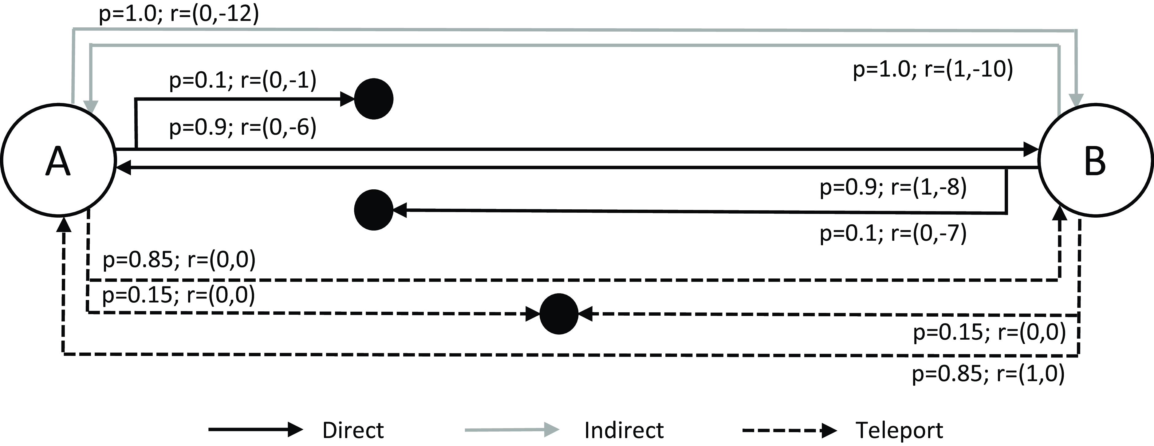
Figure 1. The Space Traders MOMDP. Solid black lines show the Direct actions, solid grey line show the Indirect actions, and dashed lines indicate Teleport actions. Solid black circles indicate terminal (failure) states (Vamplew et al., Reference Vamplew, Foale and Dazeley2022a)
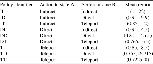
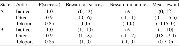
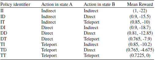
Table 1 shows the transition probabilities, immediate reward for each state-action pair and mean rewards as well. The reason for selecting Space Traders as the testing environment is because it is a relatively small environment. So, it is easy to list all of the nine possible deterministic policies which are shown in Table 2. For these experiments we assume the goal of the agent is to minimise the time taken to complete the travel as well as having at least equal or above 88% probability of successful completion (i.e. we are using TLO, with a threshold applied to the success objective). Under this utility function, the optimal policy is DI as it is the fastest policy which achieves a mean return of 0.88 or higher for the first objective.
Table 1. The probability of success and reward values for each state-action pair in the Space Traders MOMDP (Vamplew et al., Reference Vamplew, Foale and Dazeley2022a)
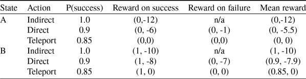
Table 2. The mean return for the nine available deterministic policies for the Space Traders Environment (Vamplew et al., Reference Vamplew, Foale and Dazeley2022a)
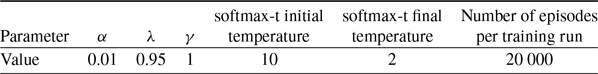
The hyperparameters used for experiments on the Space Traders environment can be found in Table 3. These were kept the same across all experiments so as to facilitate fair comparison between the different approaches. For exploration we use a multi-objective variant of softmax (softmax-t) (Vamplew et al., Reference Vamplew, Dazeley and Foale2017).
Table 3. Hyperparameters used for experiments with the Space Traders environment
In some of the following experiments we will introduce variations of the original Space Traders environment in order to demonstrate that methods solving the original problem may fail under small changes in environmental or reward structure, illustrating that they do not provide a general solution to the problem of learning SER-optimal policies.
3.4 Scope
We have made several decisions to restrict the scope of this study, so as to focus on the specific issues of interest (solving SER-optimality for stochastic state transitions, and analysing the impact of noisy estimates on MOQ-learning).
These issues can arise both in the context of single-policy and multi-policy MORL, but here we consider only single-policy approaches to simplify the analysis. Similarly we examine only a single choice of utility function—TLO was selected as it has been widely used in the MORL literature (Gábor et al., Reference Gábor, Kalmár and Szepesvári1998; Hayes et al., Reference Hayes, Howley and Mannion2020; Issabekov & Vamplew, Reference Issabekov, Vamplew, Thielscher and Zhang2012; Jin & Ma, Reference Jin and Ma2017; Dornheim, Reference Dornheim2022; Tercan, Reference Tercan2022; Lian et al., Reference Lian, Lv and Lu2023), and has previously been shown to be particularly sensitive to noisy Q-value estimates (Vamplew et al., Reference Vamplew, Foale and Dazeley2022a). Finally, the simplicity of the Space Traders task allows us to use a tabular form of MOQ-learning, meaning that the noisiness of the estimates arises directly from the stochasticity of the environment. The problems identified in this study would be expected to be even more prevalent for Deep MORL methods, where the use of function approximation introduces an additional source of error for the Q-values.
4. Experimental results—baseline MOQ-learning
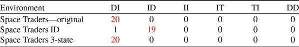
This experiment used the baseline MOQ-learning algorithm. The aim was to confirm the original findings of Vamplew et al. (Reference Vamplew, Foale and Dazeley2022a), and provide a baseline for the later experiments. Table 4 summarises the distribution of the final greedy policy learned over twenty independent training results.
Table 4. The final greedy policies learned in twenty independent runs of the baseline multi-objective Q-learning algorithm (Algorithm 1) on the Space Traders environment
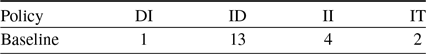
The empirical results show that the desired optimal policy (DI) was not converged to in practice, with it being identified as the best policy in only one of twenty runs. This is comparable with the results reported for this method by Vamplew et al. (Reference Vamplew, Foale and Dazeley2022a). They explained this behaviour by noting that regardless of which action the agent selected at state A, if state B is successfully reached, then a zero reward will have been received by the agent for the first objective. In other words, the accumulated expected reward for the first objective at state B is zero. Therefore, the choice of action at state B is purely based on the action values at that state. Now looking at the mean action values for state B which is reported in Table 1, it can be seen that the teleport action will be eliminated because it fails to meet the threshold for the first objective, and the direct action will be preferred over indirect action as both meet the threshold, and direct action takes less time penalty in second objective. Therefore, the agent will choose the direct action at state B regardless of which action the agent selected at state A. As the result, this agent at state A will only consider Policy ID, DD and TD and only policy ID is above the threshold for the first objective if we look back the mean reward in Table 2. Therefore the agent converges to the suboptimal policy ID in most trials.
In addition the issue of noisy estimates means that the agent will sometimes settle on another policy, including a policy which does not even meet the success threshold. This is illustrated in Figure 2 which visualises the learning behaviour of the baseline method (Algorithm 1) during four of the twenty trials, selected so as to include one example of each of the four different final policies learned by this algorithm, as listed in Table 4. Each subpart of the figure illustrates a single run of the baseline algorithm. For each episode, the policy which the agent believed to be optimal at that stage of its learning is indicated by a blue bar. The green dashed line indicates the threshold for the first objective. The policies on the vertical axis are sorted to indicate that only the DI, ID and II policies meet this constraint. As we can see from all of these policy charts, the agent’s behaviour is unstable with frequent changes in its choice of optimal policy. Policy ID is the most frequently selected across 20 000 episodes, which reflects why it is the most frequent final outcome, but in many runs the agent winds up with a different final policy. In particular, it can be seen that policies beneath the threshold are regarded as optimal on an intermittent basis, which indicates that the agent’s estimate of the value of these policies must be inaccurate.
To highlight the impact of noisy estimates, we ran a further twenty trials during which the learning was linearly decayed from its initial learning rate to zero. All other hyperparameters were the same as in the previous trials of the baseline algorithm. Decaying the learning rate will minimise the impact of the environmental stochasticity on the variation of the agent’s Q-values, and should result in increased stability in the choice of greedy policy. Table 5 summarises the final policies learned during these trials, while Figure 3 visualises the choice of greedy policy over two representative trials, one with a constant learning rate and one with a decayed learning rate. Both of these trials culminate in the final greedy policy being ID.
Table 5. The final greedy policies learned in twenty independent runs of baseline multi-objective Q-learning (Algorithm 1) with constant or decayed learning rates for the Space Traders environment
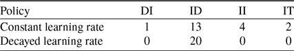
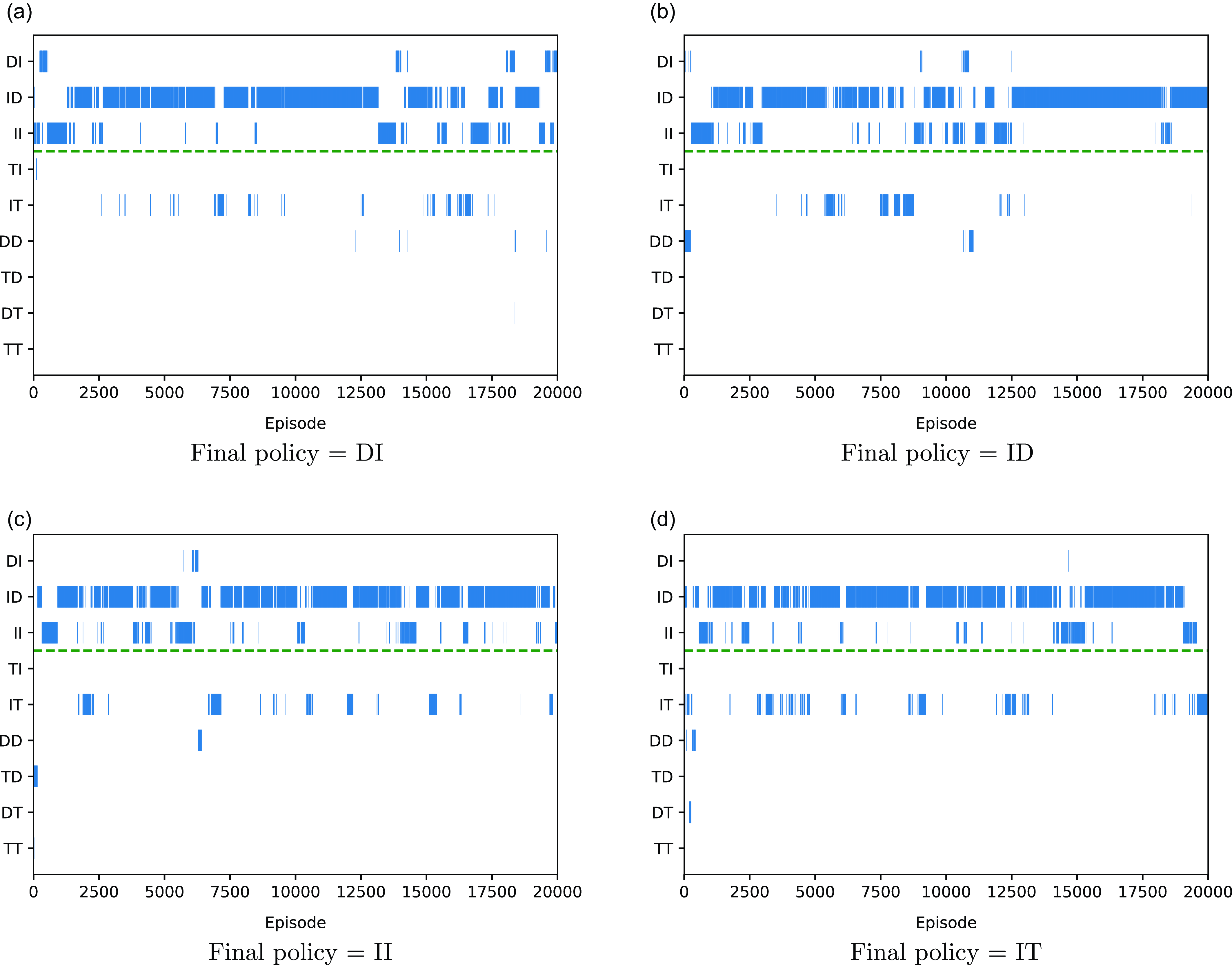
Figure 2. Policy charts showing the greedy policy produced by the baseline multi-objective Q-learning algorithm (Algorithm 1) on the Space Traders environment. Each chart shows the greedy policy identified by the agent at each episode of four different trials, culminating in different final policies. The dashed green line represents the threshold used for TLO, to highlight which policies meet this threshold
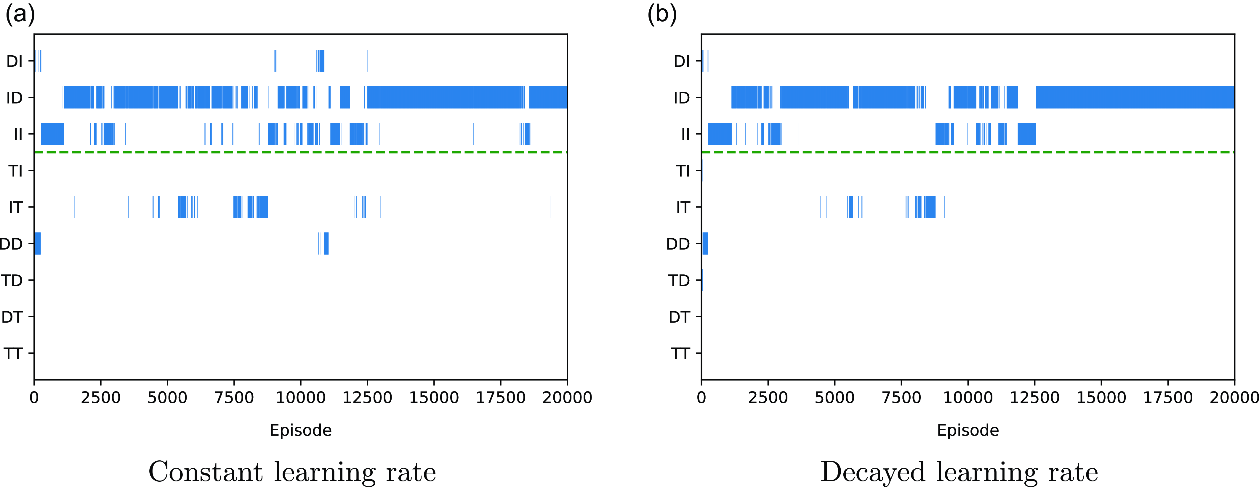
Figure 3. The Policy chart for baseline method with a decayed learning rate in the Space Traders Environment
As can be seen from Table 5, the decayed learning rate does indeed result in more stable and consistent learning behaviour, as the agent converges to the same final policy in all twenty trials, compared to the diverse set of final policies evident under a constant learning rate. The policy chart in Figure 3 also indicates that gradually decaying the learning rate reduces the influence of the environmental stochasticity. After 15 000 episodes, the agent converges to a single fixed greedy policy until the end of the experiment. So clearly the decayed learning rate helps to eliminate the impact of environmental stochasticity on this agent, allowing it to reliably converge to the same solution. However this also highlights the inability of the baseline method to learn SER-optimal behaviour, as it consistently converges to the suboptimal policy ID in all twenty trials, never finding the desired DI policy.
The results in this section of the study reveal two main findings:
-
• The baseline MOQ-learning algorithm fails to learn the SER-optimal policy in the majority of trials (confirming the findings of Vamplew et al., Reference Vamplew, Foale and Dazeley2022a).
-
• The noisy estimates arising from environmental stochasticity lead to instability in the greedy policy learned by MOQ-learning, with variations both within and between trials.
For clarity, the next two sections of the paper will focus on the first issue, by examining algorithmic modifications designed to allow learning of the SER-optimal policy. We will present results of these approaches in conjunction with the use of a decayed learning rate, so that the performance of each approach can be assessed relatively independently of the noisy estimates issue. We will return to the issue of noisy estimates in the latter half of Section 7. Results and discussion for the approaches covered in Sections 5 and 6 with a constant learning rate are available in Appendix A.
5. Reward engineering
In the remainder of the paper we examine various approaches for addressing the inability of the baseline MOQ-learning algorithm to reliably identify the SER-optimal policy for the Space Traders environment. The first approach we consider is to modify the reward structure of Space Traders, while retaining the same environmental dynamics. While the dynamics of state transitions is an intrinsic component of the environment, the reward function is generally specified by a human designer, with the aim of producing the desired behaviour from the agent. Therefore modifying the reward structure is within the designer’s control, and a better-designed reward signal may allow for improved performance by the agent. Therefore, the most simple and natural approach is to modify the reward structure first without actually changing the original MOQ-learning algorithm.
5.1 Modified reward structure and results
A version of Space Traders with a modified reward design is shown in Figure 4—we will refer to this as Space Traders MR. The agent will receive a -1 reward for the first objective when visiting one of the terminal states, receive +1 when reaching the goal state, and 0 for other intermediate transitions. The motivation here is to provide additional information to the agent at State A regarding the likelihood of any action leading to a terminal state. As can be seen from the top-half of Table 6, under the new reward design, the three actions from state A have differing mean immediate rewards for the first objective of 0, -0.1, and -0.15.
Table 6. The probability of success and reward values for each state-action pair in Space Traders MR
As a consequence, the threshold value of the utility function also needs to be updated, because the total rewards for the first element are now ranging from -1 to 1 instead of 0 to 1. Adjusting for this change in range results in a revised threshold equal to
 $0.88*1+0.12*(\!-1)=0.76$
. All other algorithmic settings remain the same as in Section 4.
$0.88*1+0.12*(\!-1)=0.76$
. All other algorithmic settings remain the same as in Section 4.
As shown in Table 7, the MOQ-learning agent using the modified reward signal and a decayed learning rate converges to the optimal DI policy in all 20 trials. The policy chart in Figure 5(a) shows the agent learns quite stably, settling on the optimal policy without deviation after about 16,000 episodes.
Table 7. The final greedy policies learned in twenty independent runs of the Algorithm 1 with a decayed learning rate for Space Traders MR environment, compared to the original Space Traders environment
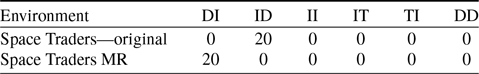

Figure 4. The Space Traders MR environment, which has the same state transition dynamics as the original Space Traders but with a modified reward design. The changed rewards have been highlighted in red
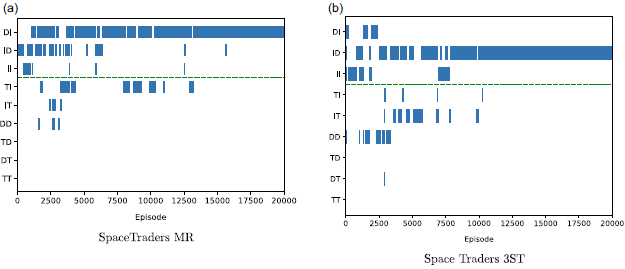
Figure 5. Policy charts for MOQ-learning on the Space Traders MR and 3ST environments. Chart (a) shows convergence to the SER-optimal DI policy on Space Traders MR, whereas (b) shows convergence to the suboptimal ID policy when applying the same algorithm and reward design to the Space Traders 3ST environment
5.2 Space Traders with modified state structure
The results in the previous section show that modifying the reward structure to explicitly provide a negative reward component on transitions to fatal terminal states allows for improved performance from the MOQ-learning algorithm on the SpaceTraders environment. However in order for this approach to be useful, we need to confirm that similar reward structures which capture relevant information about transitions to terminal states are possible regardless of the structure of the environment and its state dynamics.
To investigate this, we introduce a variant of the Space Traders environment with an additional state as shown in Figure 6—this will be referred to as Space Traders 3-State (3ST). It includes a new state C reached when the agent selects the direct action at state A. This introduces a delay between the selection of the direct action at A, and the ultimate reaching of the terminal state (and consequent negative reward for the first objective).
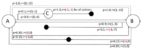
Figure 6. The Space Traders 3-State environment which adds an additional state C to the Space Traders MOMDP with a more complex state structure. All the changes have been highlighted in red color
The empirical results from twenty trials in Table 8 show that the desired optimal policy (DI) was not converged to in practice for the Space Traders 3-State environment. A closer examination of the behaviour of the agent on Space Traders MR shows that at state B the agent will have different accumulated expected reward for the first objective depending on which action was chosen at State A. For example, if the agent selects the Direct action and successfully reaches state B, the ideal accumulated expected reward for the first objective will be
 $0.9*0+0.1*(\!-1)=-0.1$
when the action values are learned with sufficient accuracy. This will lead the agent to select the indirect action in state B. But in the Space Traders 3-State variant environment, the accumulated expected reward will be zero when the agent reaches state B by taking direct action (as was also the case for the original Space Traders MOMDP). As a result, the agent converges to the suboptimal policy ID in practice again.
$0.9*0+0.1*(\!-1)=-0.1$
when the action values are learned with sufficient accuracy. This will lead the agent to select the indirect action in state B. But in the Space Traders 3-State variant environment, the accumulated expected reward will be zero when the agent reaches state B by taking direct action (as was also the case for the original Space Traders MOMDP). As a result, the agent converges to the suboptimal policy ID in practice again.
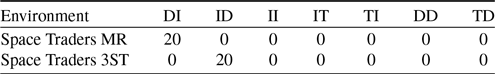
Table 8. The final greedy policies learned in twenty independent runs of the Algorithm 1 for Space Traders 3-State environment, compared to the Space Traders MR environment. All runs used a decayed learning rate
This example illustrates that while it may be possible in some cases to encourage SER-optimal behaviour via a careful designing of rewards, more generally the structure of the environment may make it difficult or impossible to identify a suitable reward design. The modified reward used for Space Traders MR was based on a simple principle of providing a -1 reward for the success objective on any transitions to a terminal state. For this particular environment structure, this reward signal essentially captures the required information such as the transition probabilities within the accumulated expected reward for the first objective. However, as shown by the Space Traders 3-State variant, this reward design principle is not sufficient in general. Therefore, relying on the reward designer being able to create a suitable reward structure is insufficient to provide a general means to address issues in stochastic environments under SER criteria.
6. Incorporation of global statistics
As identified previously, the main issue for applying MOQ-learning algorithm to stochastic environment is that the action selection at given state is purely based on local information (the Q values for the current state) and current episode information (accumulated expected reward) (Vamplew et al., Reference Vamplew, Foale and Dazeley2022a). This is the same issue previously identified for multi-objective planning algorithms by Bryce et al. (Reference Bryce, Cushing and Kambhampati2007). However, in order to maximise the expected utility over multiple episodes (SER criteria) the agent must also consider the expected return on other episodes where the current state is not reached. In other words, the agent must also have some level of knowledge about global statistics in order to maximise scalarised expected return (SER). Therefore, the second approach we examine is to include extra global information within the MOQ-learning algorithm.
Algorithm 2 The multi-objective stochastic state Q(
 $\lambda$
) algorithm (MOSS Q-learning). Highlighted text identifies the changes and extensions introduced relative to multi-objective Q(
$\lambda$
) algorithm (MOSS Q-learning). Highlighted text identifies the changes and extensions introduced relative to multi-objective Q(
 $\lambda$
) as previously described in Algorithm 1.
$\lambda$
) as previously described in Algorithm 1.
6.1 Multi-objective Stochastic State Q-learning (MOSS)
To support this idea, Multi-objective Stochastic State Q-learning (MOSS)(Algorithm 2) is introducedFootnote 3 . Here are the changes compared with previous MOQ-learning (Algorithm 1)
-
• The agent maintains two pieces of global information: the total number of episodes experienced (
$v_\pi$
), and an estimate of the average per-episode return (
$E_\pi$
)—implemented by lines 7, 8, 10, and 40 of Algorithm 2. -
• For every state, the agent maintains a counter of episodes in which this state was visited at least once (v(s) which is updated by line 2 of Algorithm 3), and the estimated average return in those episodes (E(s)—lines 41–43 of Algorithm 2)).
-
• Action selection is based on
$U(S^A_t)$
which for each action in the current augmented state, estimates the mean per-episode vector return for a policy which selects that action in this augmented state. Importantly the value of U is determined not just by the returns of episodes in which
$s^A_t$
arises, but also by the returns of episodes which do not encounter this augmented state. The calculations to achieve this are performed by Algorithm 3.


-
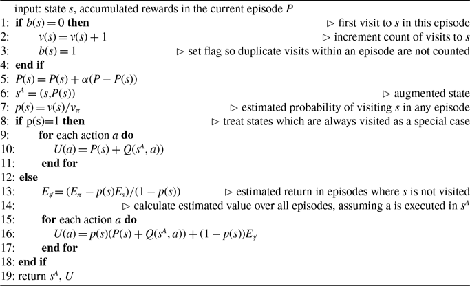
− Estimate the mean accumulated vector return when the current state is reached P(s) (line 5)
-
− Estimate the probability of encountering the current state in any episode p(s) (line 7)
-
− In the special case that
$p(s)=1$
(i.e. this state is always reached), U can be calculated directly as the sum of P(s) and
$Q(s^A,a)$
(line 10, which is equivalent to line 18 in Algorithm 1—the difference is that in the latter case, this process is used for all states). -
− In the more general case where
$p(s)\lt1$
(i.e. the state is only sometimes encountered, due to stochasticity), U is calculated in two steps:


-
* The mean vector return for episodes in which s does not occur (
$E_{\not{s}}$
) is estimated based on the estimated return over all episodes
$E_\pi$
, the estimated return in episodes in which s does occur
$E_s$
, and the probability of s occurring p(s) (line 13) -
* The estimated return vector of this action in episodes when state s does arise (P(s) +
$Q(s^A,a)$
) is combined with the estimated return vector for episodes in which s does not occur (
$E_{\not{s}}$
) via a probability-weighted average (lines 15–16).


Essentially U provides a holistic, non-local measure of the value for each action in each state. Using this value rather than the purely local measure (
 $P(s) + Q(s^A,a)$
) aims to make action-selection more compatible with the goal of finding the SER-optimal policy.
$P(s) + Q(s^A,a)$
) aims to make action-selection more compatible with the goal of finding the SER-optimal policy.
Algorithm 3 The update-statistics helper algorithm for MOSS Q-learning (Algorithm 2). Given a particular state s it updates the global variables which store statistics related to s. It will then return an augmented state formed from the concatenation of s with the estimated mean accumulated reward when s is reached, and a utility vector U which estimates the mean vector return over all episodes for each action available in s
6.2 MOSS Q-learning results
The results in Table 9 show that the MOSS algorithm performs successfully on the SpaceTraders environment when applied in conjunction with a decayed learning rate. The agent converges to the optimal DI policy in all twenty runs. The policy chart in Figure 7 is drawn from a representative run, and shows that MOSS stabilises on the desired optimal policy DI and doesn’t deviate from it after around 15 000 epsiodes.
Table 9. The final greedy policies learned in twenty independent runs of the MOSS algorithm with a decayed learning rate for both the Space Traders and Space Traders ID environments. Red text highlights the SER-optimal policy for each environment
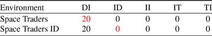
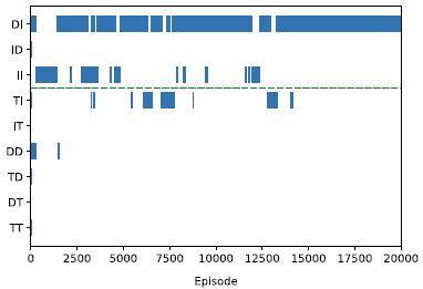
Figure 7. The Policy chart for the MOSS algorithm with the decayed learning rate in original Space Traders Environment
In order to further test the MOSS algorithm we introduce a further variant of the Space Traders Problem (Space Traders ID) as shown in Figure 8.
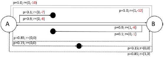
Figure 8. The Space Traders ID variant environment. All the changes compared with original have been highlighted in red. The changed rewards result in ID being the SER-optimal policy for this environment
All the changes compared with original one have been highlighted in red. The main difference is that the time penalty for each action has been swapped from state A to state B. The new probability of success and reward values for each state-action pair in the new variant Space Traders are shown in Table 10. The only difference between policies DI and ID in the original Space Traders Problem is the second objective—the time penalty. Therefore in this new variant of Space Traders problem, policy ID has become the desired SER-optimal policy as we can see from Table 11.
Table 10. The probability of success and reward values for each state-action pair in the new variant Space Traders ID environment
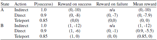
Table 11. Nine available deterministic policies mean return for Space Traders ID environment
A closer examination of the MOSS algorithm (Algorithm 2) reveals that the estimated values used for action-selection (
 $s_t$
,
$s_t$
,
 $P(s_t)$
,
$P(s_t)$
,
 $p(s_t)$
, and
$p(s_t)$
, and
 $E_{\not{s_{t+1}}}$
) should be based only on the trajectories produced during execution of the greedy policy, whereas in the current algorithm they are derived from all trajectories. As a result, the estimated probability of visiting state s in any episode
$E_{\not{s_{t+1}}}$
) should be based only on the trajectories produced during execution of the greedy policy, whereas in the current algorithm they are derived from all trajectories. As a result, the estimated probability of visiting state s in any episode
 $p(s_t)$
is below 1 because of exploratory actions. In turn, the U(a) values at state B for the direct and teleport actions are below threshold for first objective. So it can already be seen that this agent will not converge to the desired policy ID.Footnote
4
$p(s_t)$
is below 1 because of exploratory actions. In turn, the U(a) values at state B for the direct and teleport actions are below threshold for first objective. So it can already be seen that this agent will not converge to the desired policy ID.Footnote
4
The results in Table 9 show that, for the original Space Traders environment, the combination of the MOSS algorithm and a decayed learning rate does reliably converge to the correct SER-optimal policy DI. However when we apply them to Space Traders ID, the agent fails to learn the desired optimal policy ID. Therefore the MOSS algorithm is not an adequate solution to the problem of learning SER-optimal policies for stochastic MOMDPs.
7. Policy-options
7.1 Policy-options algorithm
The final approach we examine to address the issue of SER-optimality is inspired by the concept of options. An option is a temporally-extended action, consisting of a sequence of single-step actions which the agent commits to in advance, as opposed to selecting an action on each time-step (Sutton et al., Reference Sutton, Precup and Singh1999). The agent selects an option and executes the sequence of actions defined by it, while continuing to observe states and rewards on each time-step, and learning the Q-values associated with the fine-grained actions.
Algorithm 4 multi-objective Q(
 $\lambda$
) with policy-options.
$\lambda$
) with policy-options.
The use we make of options here differs from their usual application. The simplicity of the original Space Traders environment (2 states, 3 actions per state) means it is possible to define nine options corresponding to the nine deterministic policies which we know exist for this environment. At the start of each episode the agent selects one of these policy-options to perform, and pre-commits to following that policy for the entire episode. Therefore, rather than learning state-action values for all states, it is sufficient for the agent to just learn option values for the starting state (State A). Over time the state-option values the agent has learnt at state A should match the mean rewards for each of the nine deterministic policies in Table 2. This policy-options approach is detailed in Algorithm 4 Footnote 5 .
Performing action-selection in advance based on the estimated values of each policy eliminates the local decision-making at each state which has been identified as the cause of the issues which methods like multi-objective Q-learning have in learning SER-optimal policies (Bryce et al., Reference Bryce, Cushing and Kambhampati2007; Vamplew et al., Reference Vamplew, Foale and Dazeley2022a). Clearly such an approach is infeasible for more complex environments, as the number of deterministic policies will equal
 ${|A|}^{|S|}$
and so grows extremely rapidly as the number of actions and states extends beyond the 3 actions and 2 states which exist in SpaceTraders. However applying this approach to this simple environment provides a clear indication of the role which local action-selection plays in hampering attempts to learn SER-optimal behaviour.
${|A|}^{|S|}$
and so grows extremely rapidly as the number of actions and states extends beyond the 3 actions and 2 states which exist in SpaceTraders. However applying this approach to this simple environment provides a clear indication of the role which local action-selection plays in hampering attempts to learn SER-optimal behaviour.
7.2 Policy-options experimental results
The results in Table 12 demonstrate that, as expected, the policy-options approach is effective. Eliminating local decision-making by committing to the entire policy at the start of each episode enables this approach to converge to the optimal policy in all but one trial across all variants of the SpaceTraders environment. This shows that unlike the earlier approaches which failed on some of these variants, policy-options is a reliable approach across all of the tested environments.
Table 12. The final greedy policies learned in twenty independent runs of the policy-options MOQ-Learning algorithm for the variants of the Space Traders environment, with a decayed learning rate—red indicates the SER-optimal policy for each variant
When combined with decaying the learning rate, policy-options learning is able to address both the local decision-making issue and the problem of noisy Q-value estimates for stochastic environments. However this method suffers from a more fundamental problem—the curse of dimensionality. For problems with more states and actions, the number of pre-defined options are going to increase exponentially, and so this method is not able to scale up to solve more complex problems in real-life.
7.3 Policy-options and noisy estimates
As shown in the previous section, because the policy-options method eliminates any local decision-making, it nearly always converges to the SER-optimal policy when used in conjunction with a decayed learning rate. This provides an opportunity to more closely examine the effect of noisy estimates on the behaviour of an MORL agent. By re-applying the policy-options algorithm to each of the Space Traders environment but this time using a constant learning rate, we can isolate the impact of the noisy estimates induced by that form of learning rate.
Table 13 shows the distribution of the final policy learned under these settings on the original SpaceTraders environment and its variants. When compared against the performance of the same agent with a decayed learning rate from Table 12, it can be seen that the noise in the estimates caused by the large constant learning rate substantially hinders the agent, which converges to a non-optimal policy in multiple runs.
Table 13. A comparison of the final greedy policies learned in twenty independent runs of the policy-options MOQ-Learning algorithm for the Space Traders environment variants, with either a decayed or constant learning rate—red indicates the SER-optimal policy for each variant
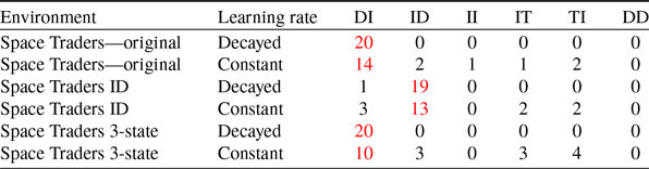
Figure 9 highlights the noisy estimates issue as it can be seen that the policy identified as being optimal fluctuates on a frequent basis during learning when the learning rate is constant, and quite often includes policies which fail to achieve the threshold on the first objective. Seeing as both the agent’s value estimates and action-selection are being performed at the level of complete policies, this can only arise due to errors in those estimated values arising from the stochastic nature of the environment.
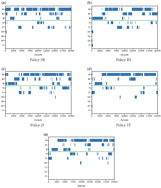
Figure 9. Policy charts for five sample runs of the policy-options MOQ-Learning algorithm with a constant learning rate on Space Traders
Figure 10 visualises a single trial of policy-options for the original Space Traders problem which eventually selects policy TI. The first layer is the normal policy chart where each policy has been assigned a unique colour for clarity. The middle layer indicates the Q-value at state A for the first objective, and the bottom layer shows the Q-value at state A for the second objective. As we can see from these three graphs, due to the combination of the stochastic environment, the constant learning rate, and the utility function’s hard threshold, the agent’s greedy policy never stabilised even though it stays on the desired optimal policy DI most of time. There is an extreme case just before 10 000 episodes and again at around 18 000 episodes, where the policy DD (in brown color) has several unlikely successes in a row, and its estimated value rises above the threshold. This means it is temporarily identified as the optimal policy in the policy chart at those times, despite in actuality being the least desirable policy—this indicates the extent of the impact of noisy estimates within a highly stochastic environment such as Space Traders.
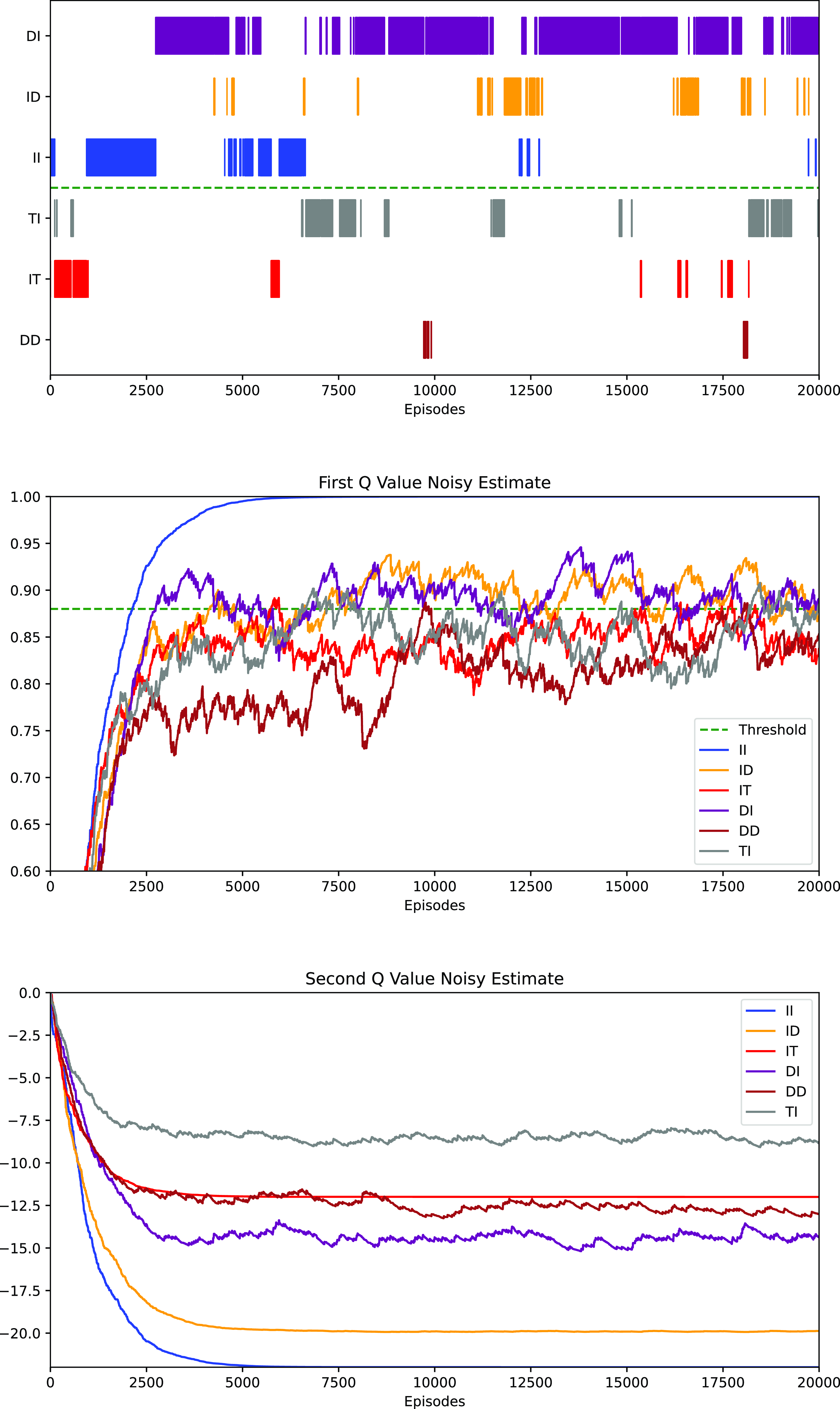
Figure 10. The Noisy Q Value Estimate issue in policy-options MOQ-learning with a constant learning rate. These graphs illustrate agent behaviour for a single run. The top graph shows which option/policy is viewed as optimal after each episode, while the lower graphs show the estimated Q-value for each objective for each option
8. Conclusion
Multi-objective Q-learning is an extension of scalar value Q-learning that has been widely used in the MORL literature. However it has been shown to have limitations in terms of finding the SER-optimal policy for environments with stochastic state transitions. This research has provided the first detailed investigation into the factors that influence the frequency with which value-based MORL Q-learning algorithms learn the SER-optimal policy under a non-linear scalarisation function for an environment with stochastic state transitions.
8.1 Major findings
This study explored three different approaches to address the issues identified by Vamplew et al. (Reference Vamplew, Foale and Dazeley2022a) regarding the inability of multi-objective Q-learning methods to reliably learn the SER-optimal policy for environments with stochastic state transitions. The first approach was to apply reward design methods to improve the MORL agent’s performance in stochastic environments. The second approach (MOSS) utilised global statistics to inform the agent’s action selection at each state. The final approach was to use policy-options (options defined at the level of complete policies).
The results for the first approach showed that with a new reward signal which provided additional information about the probability of transitioning to terminal states, standard MOQ-learning was able to find the desired optimal policy in the original Space Traders problem. However, using a slightly modified variant of Space Traders we demonstrated that in general it may be too hard or even impossible to design a suitable reward structure for any given MOMDP.
It was found in the second approach that the augmented state combined with use of global statistics in the MOSS algorithm clearly outperformed the baseline method for the Space Traders problem. However, the MOSS algorithm fails to find the correct policy for the Space Traders ID variation of the environment, and therefore does not provide a reliable solution to the task of finding SER-optimal policies.
The results for the third approach reveal that policy-option learning is able to identify the optimal policy for the SER criteria for a relatively small stochastic environment like Space Traders. However clearly this method still fails from a more fundamental problem—the curse of dimensionality means it is infeasible for environments containing more than a small number of states and actions.
The key contribution of this work is isolating the impact of noisy Q-estimates on the performance of MO Q-learning methods. The final experiments using policy-options clearly illustrated the extent to which noisy estimates can disrupt the performance of MO Q-learning agents. By learning Q-values and performing selection at the level of policies rather than at each individual state, this approach avoids the issues with local decision-making which are the primary cause of difficulty in learning SER-optimal policies (Bryce et al., Reference Bryce, Cushing and Kambhampati2007; Vamplew et al., Reference Vamplew, Foale and Dazeley2022a). However the empirical results showed that when used in conjunction with a constant learning rate, the variations in estimates introduced by the stochasticity in the environments lead to instability in the agent’s greedy policy. In many cases this meant the final greedy policy found at the end of learning was not the SER-optimal policy.
These results highlight that in order to address the problems of value-based MORL methods on stochastic environments, it will be essential to solve both the local decision-making issue and also the noisy estimates issue, and that a decaying learning rate may be valuable in addressing the latter.
8.2 Implications for MORL research and practice
The main implication of these findings is that value-based MORL algorithms may be unable to be effectively applied for the combination of optimising the SER-criteria with a non-linear utility in stochastic environments. This does not necessarily invalidate prior work on value-based MORL, as in many cases that research was not addressing this specific combination of factors. For example, many value-based MORL approaches assume linear utility (Abels et al., Reference Abels, Roijers, Lenaerts, Nowé and Steckelmacher2019; Yang et al., Reference Yang, Sun and Narasimhan2019; Xu et al., Reference Xu, Tian, Ma, Rus, Sueda and Matusik2020; Basaklar et al., Reference Basaklar, Gumussoy and Ogras2022; Alegre et al., Reference Alegre, Bazzan, Roijers, Nowé and da Silva2023). The approach of Cai et al. (Reference Cai, Zhang, Zhao, Bian, Sugiyama and Llorens2023) learns scalarised returns rather than vectors and so is targeting ESR-optimality. Similarly Tessler et al. (Reference Tessler, Mankowitz and Mannor2018) and Skalse et al. (Reference Skalse, Hammond, Griffin and Abate2022) address optimising a utility function akin to TLO, but in the context of ESR rather than SER. Meanwhile the Pareto-conditioned network of Reymond et al. (Reference Reymond, Bargiacchi and Nowé2022) is restricted to deterministic environments. However our findings have implications for possible extensions of these methods. For example, a seemingly obvious means of implementing multi-policy learning for non-linear SER utility might be to merge the augmented state and action-selection methods from MO Q-learning (Algorithm 1) with the conditioned network structure of Abels et al. (Reference Abels, Roijers, Lenaerts, Nowé and Steckelmacher2019), conditioning on the parameters of the utility function. However the results of our experiments indicate that this approach is likely to fail if applied to stochastic environments.
The issues identified in this research may have been previously unreported in part because of the limitations of MORL benchmarks, which have in the past had limited coverage of stochasticity. For example the first widely-adopted set of benchmark environments from Vamplew et al. (Reference Vamplew, Dazeley, Berry, Issabekov and Dekker2011) features three fully-deterministic environments (Deep Sea Treasure, MO-Puddleworld and MO-MountainCar) and one with just a single state with a stochastic transition and reward (Resource Gathering). The recent benchmark suite of MO-Gymnasium (Felten et al., Reference Felten, Alegre, Nowé, Bazzan, Talbi, Danoy and da Silva2023) improves this situation by introducing some environments featuring stochasticity, but even here this is often limited to adding noise to the starting states (as in Four Room, and the MuJoCo tasks).
While the Space Traders environment and the variants thereof were sufficient to demonstrate the limitations of the approaches tested in this study by providing counter-examples where these approaches failed, more broadly this is not a sufficient benchmark for future MORL studies. There is a need for a suite of MORL benchmark environments which exhibit a range of stochasticity in both rewards and state transitions, with a more challenging size of state and action spaces than exhibited by Space Traders. Ideally these will be implemented within the MO-Gymnasium framework so as to facilitate widespread adoption (Felten et al., Reference Felten, Alegre, Nowé, Bazzan, Talbi, Danoy and da Silva2023).
8.3 Future work
There are two issues existing for MO Q-learning in stochastic environments—the core stochastic SER issue caused by local decision-making and also the noisy Q value estimates. Therefore a successful algorithm must address both of those problems together. Due to the flaws in each investigated method, none of them could be directly applied into real-world applications, and so there is a need for further research to develop more reliable approaches for SER-optimal MORL.
The first recommendation for future research is to look at policy-based methods such as policy gradient RL. As these methods directly maximise the policy as a whole by defining a set of policy parameters, therefore they do not have the local decision-making issue faced by model-free value-based methods such as MOQ-learning. Several researchers have developed and assessed policy-based methods for multi-objective problems (Parisi et al., Reference Parisi, Pirotta, Smacchia, Bascetta and Restelli2014; Bai et al., Reference Bai, Agarwal and Aggarwal2021). In the work which inspired our study, Vamplew et al. (Reference Vamplew, Foale and Dazeley2022a) argued that most policy-based MORL methods produce stochastic policies, whereas in some applications deterministic policies may be required. However, recently Röpke et al. (Reference Röpke, Reymond, Mannion, Roijers and Nowé2024) reported that in practice the policy-gradient algorithms they applied to non-linear MORL typically converged toward deterministic policies during learning, and that determinism could be enforced at the policy execution stage.
A second promising research direction is to investigate distributional reinforcement learning (DRL). Conventional value-based RL learns a single value per state-action pair which represents the expected return. Distributional reinforcement learning on the other hand works directly with the full distribution of the returns instead. This can be beneficial for MORL, as shown by Hayes et al. (Reference Hayes, Roijers, Howley and Mannion2022a) who applied Distributional Multi-objective Value Iteration to find optimal policies for the ESR criteria. The additional information about the rewards captured by DRL algorithms could potentially prove useful in overcoming both the noisy estimates and stochastic SER issues.
We also note that while the specific form of policy-options used in Section 7 is not practical due to its poor scaling to larger state or actions spaces, more sophisticated forms of options may be applicable. In particular, approaches to options discovery based on successor representations and successor features (Kulkarni et al., Reference Kulkarni, Saeedi, Gautam and Gershman2016; Machado et al., Reference Machado, Barreto, Precup and Bowling2023) allow automated discovery of options without designer intervention, and may enable application of the approach described in Section 7 to larger real-world problems. We speculate that a dynamic options algorithm may be able to constrain the agent to only switch options when in a state which has only deterministic state transitions (this is not possible for Space Traders as both non-terminal states lead to stochastic transitions). For environments with a limited amount of stochasticity this may allow options-based algorithms to scale sufficiently to be practical for finding SER-optimal policies.
Data availability statement
The experimental data that supports the findings of this study are available in Figshare with the identifier https://doi.org/10.25955/24980382
Competing interests
The authors declare that they have no conflict of interest.
Appendix A. Additional Results with a Constant Learning Rate
Sections 5 and 6 presented experimental results for the reward engineering and MOSS approaches. Those experiments were based on a decayed learning rate, so as to allow the underlying capabilities of each approach to be assessed without the additional complication of noisy estimates. For completeness, this appendix reports results for these approaches using a constant learning rate, further illustrating the substantial impact of noisy estimates on the convergence stability of multi-objective Q-learning.
A.1. Reward engineering with noisy estimates
Table A1 presents the results of an MO Q-learning agent on each of the variants of the Space Traders environment from Section 5, with both a constant and a decayed learning rate. As discussed earlier in the paper, the constant learning rate tends to produce noisier and more variable value estimates than a decayed learning rate, so this table highlights the negative impact that this noise has on the agent’s performance.
As we can see from Table A1, for both variants of the environment, learning with a decayed learning rate results in consistent convergence to a single policy (for Space Traders MR this is the optimal DI policy, whereas for SpaceTraders 3ST it is a suboptimal policy, as previously discussed in Section 5). In contrast, when a constant learning rate is used, the resulting noisy estimates produce much less consistent outcomes.
Table A1. The final greedy policies learned in twenty independent runs of the Algorithm 1 for Space Traders 3-State environment, compared to the Space Traders MR environment

This is particularly problematic in the case of Space Traders MR runs, where the agent with a decayed learning rate converges to the optimal DI policy in all runs. The most common outcome for the agent using a constant learning rate is the desired DI policy. However this occurs in only 10 of 20 runs. The ID policy (5 repetitions) is the second most common outcome, and other policies also occur in some runs. From Figure A1, most of time across 20 000 episodes, the agent prefers policy DI which is the desired optimal policy. However the intermittent identification of the other policies as optimal means that overall this approach still only yields the correct policy 50% of the time. It is also worth noting that this reward structure results in an even greater variety of suboptimal solutions being found compared to the original reward design (see results for the baseline algorithm with constant learning rate in Table 4).

Figure A1. Policy charts for MOQ-learning with a constant learning rate on the Space Traders MR environment—each chart illustrates a sample run culminating in a different final policy
A.2. MOSS with noisy estimates
Table A2 presents the results of the MOSS Q-learning algorithm on each of the variants of the SpaceTraders environment from Section 6, with both a constant and a decayed learning rate.
As was the case for the agents discussed in the previous subsection, the MOSS agents with a decayed learning rate reliably converge to the same policy in all runs. In this case, MOSS always converges to policy DI—this is optimal for the original Space Traders environment, but not for Space Traders ID. Again, the use of a constant learning rate induces noisier Q-value estimates which in turn leads to variations in the policies to which the MOSS agent converges. On both of the variants of Space Traders, the agent occasionally converges to either the IT or TI policy rather than DI.
The policy charts in Figure A2 highlight the impact of the noisy estimates on learning stability and convergence. MOSS with a decayed learning rate successfully stabilises on the desired optimal policy DI after around 15 000 episodes, compared with the policy chart on the left where the constant learning rate agent is still struggling to stabilise the final policy right up to the end of the run.
Table A2. The final greedy policies learned in twenty independent runs of the MOSS algorithm with either a constant or decayed learning rate for both the Space Traders and Space Traders ID environments. Red text highlights the SER-optimal policy for each environment
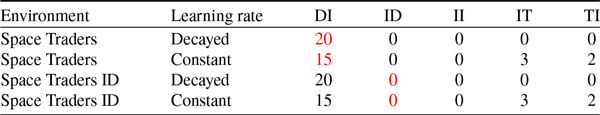
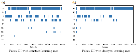
Figure A2. The Policy chart for the MOSS algorithm with either a constant or decayed learning rate in original Space Traders Environment


 Open access