2.1 Synaptic pruning in the nervous system

Biological neural networks are not engineered but self-organized, and they are able to adapt to form efficient computational structures (Johnson, Reference Johnson2001; Power and Schlaggar, Reference Power and Schlaggar2017; Yuste, Reference Yuste2015). Much of their developmental growth and adaptation depends upon pruning, where an initial overgrowth of neurons, axons, and synapses is followed by removal of inactive or inefficient components of the network (Low and Cheng, Reference Low and Cheng2006; Riccomagno and Kolodkin, Reference Riccomagno and Kolodkin2015; Sakai, Reference Sakai2020). In humans, this process begins shortly after birth; the neonatal brain contains approximately $10 \times 10^{10}$ neurons, which are pruned to $8.6 \times 10^{10}$ in the adult, a reduction of almost 15%. Similarly, the synaptic density between the neurons decreases by nearly 50% in the adult brain compared to that of a 1- to 2-year-old, following an initial growth after birth (Herculano-Houzel, Reference Herculano-Houzel2012; Sakai, Reference Sakai2020).

The cellular and molecular mechanisms underlying this pruning are numerous and highly complex, but at an abstract level they are hypothesized to be guided by certain constraints, namely metabolic energy and robustness to perturbation (Laughlin et al., Reference Laughlin, van Steveninck and Anderson1998; Herculano-Houzel, Reference Herculano-Houzel2012; Riccomagno and Kolodkin, Reference Riccomagno and Kolodkin2015; Aerts et al., Reference Aerts, Fias, Caeyenberghs and Marinazzo2016). Biological neural networks need to perform their computations with limited local and global pools of metabolic energy, which drive the networks to develop towards more efficient network topologies—that can be analyzed by means of computational tools and properties (Heiney et al., Reference Heiney, Huse Ramstad, Fiskum, Christiansen, Sandvig, Nichele and Sandvig2021)—and modes of computation and prune connections that do not contribute enough given their metabolic cost. Inversely, these networks also need to be robust against perturbations such as injury or degeneration, creating a need for redundancy and adaptability (Denève et al., Reference Denève, Alemi and Bourdoukan2017). These two constraints, working both in opposition and collectively, drive pruning in biological neural networks to network topologies that are highly efficient computational structures, such as small-world, hierarchical, and modular networks (Bassett & Sporns, Reference Bassett and Sporns2017; Sporns, Reference Sporns2013).

Moreover, these constraints differ across the brain’s many regions, which in turn drives development, including pruning, to form specialized network topologies (Sporns et al., Reference Sporns, Chialvo, Kaiser and Hilgetag2004). As different regions perform different computational tasks, the pruning mechanisms reflect this disparity by ensuring networks in, for example, sensory cortices are shaped with different inputs than those for executive or motor function. The network requirements for these computational tasks differ in terms of redundancy, parallelization, recurrency, and interregional signaling, therefore requiring different pruning targets and timescales (Meunier et al., Reference Meunier, Lambiotte and Bullmore2010; Schuldiner and Yaron, Reference Schuldiner and Yaron2015; Bordier et al., Reference Bordier, Nicolini and Bifone2017; Liao et al., Reference Liao, Vasilakos and He2017; Vézquez-Rodríguez et al., Reference Vézquez-Rodrguez, Liu, Hagmann and Misic2020). Importantly, this form of task-directed pruning stems from the same pruning mechanisms across the different regions. In general, neurons are pruned in an activity-dependent manner: low-activity neurons or synapses are marked for removal either by themselves or by microglia (glial immune cells) (Riccomagno and Kolodkin, Reference Riccomagno and Kolodkin2015; Schuldiner and Yaron, Reference Schuldiner and Yaron2015; Arcuri et al., Reference Arcuri, Mecca, Bianchi, Giambanco and Donato2017). Since the input to each region drives and shapes the activity of every neuron, the neurons and synapses which contribute to the output more often avoid pruning, allowing the region to both adapt to the input and retain the most efficient components of the network. By initially growing a large network, before pruning it down to fit the computational task, the human nervous system can adapt to multiple environments more easily than constructed or engineered networks.

Such biological findings raise questions in regards to ANN controllers for artificial agents, and in particular the identification of suitable network sizes and number of parameters needed to learn a given task. The possibility of optimizing the networks in regards to learning, robustness to noise, and other factors such as energetic cost remains still an open area of research. In the following sections, several pruning strategies for ANNs are reviewed.

2.2 Pruning in ANNs

The name ‘pruning’ is not specific to ANNs, being adapted from the decision trees, where it has been in use as early as 1984 (Breiman et al., Reference Breiman, Friedman, Stone and Olshen1984) to indicate methods of structural simplification, that is, branches pruning, of large trees having a tendency to overfit or badly generalize to unseen data. Generally, since its inception, pruning, or the top-down removal of excess pieces of architecture from a Machine Learning model, has been motivated as an aim towards simplicity, drawing parallels with Occam’s razor (Thodberg, Reference Thodberg1991; Zhang and Mühlenbein, Reference Zhang and Mühlenbein1993).

Pruning in the context of ANNs is a procedure encompassing many different techniques whose common goal is the sparsification of the network, that is, the removal of connections (synapses) between neurons, leading to a thinner subnetwork of the original model. The need for this removal can be driven by different factors: for instance, some pruning techniques have been shown to have a chance at decreasing the error committed by the model (LeCun et al., Reference LeCun, Denker, Solla, Howard and Jackel1989; Han et al., Reference Han, Pool, Tran, Dally, Cortes, Lawrence, Lee, Sugiyama and Garnett2015). It may also be of interest to shed off unnecessary structure from the ANN in order to reduce training and inference time. Additional drivers may include a better generalization capability (Bartoldson et al., Reference Bartoldson, Morcos, Barbu and Erlebacher2019) or an increased robustness (Ye et al., Reference Ye, Xu, Liu, Cheng, Lambrechts, Zhang, Zhou, Ma, Wang and Lin2019). Finally, it could be of interest to operate pruning in order to analyze symmetries between artificial and biological sparsification processes, the latter explained in Section 2.1.

ANN pruning can be subdivided in two major categories, structured or unstructured, depending upon which group(s) of connection(s) are targeted for the removal (Anwar et al., Reference Anwar, Hwang and Sung2017). Structured pruning targets well-defined formations of synapses: for example, all the connections entering one specific neuron, or, in the case of convolutional neural networks, one or more specific channels. This has immediate computational advantages as the removal of neurons or filters imply smaller parameters tensors, thus faster calculations. Conversely, unstructured pruning techniques remove connections without concern for the geometry of the deleted synapses. This leads to an irregular form of sparsity which does not directly impact the way the parameters tensors are stored in memory; thus, in order to take advantage of the smaller number of connections, specific software—like CUSPARSE (Naumov et al., Reference Naumov, Chien, Vandermersch and Kapasi2010)—or hardware—like Graphics Processing Units with dedicated sparsity support—are required (Liu et al., Reference Liu, Sun, Zhou, Huang and Darrell2019). Despite this, unstructured techniques usually lead to models performing better than the original ANN, even at high pruning rates (Frankle & Carbin, Reference Frankle and Carbin2019; Renda et al., Reference Renda, Frankle and Carbin2020), this being the reason why they can also be seen as powerful regularizers (Laurenti et al., Reference Laurenti, Patane, Wicker, Bortolussi, Cardelli and Kwiatkowska2019). In opposition to this, models pruned with structured techniques usually struggle to keep up with the performance of the unpruned network, although recent developments (Cai et al., Reference Cai, An, Yang and Xu2021) seem to have overcome this hurdle. It is to be noted, though, that even structured pruning techniques can be used as regularizers (Prakash et al., Reference Prakash, Storer, Florencio and Zhang2019), without necessarily removing the pruned parameters from the structure.

An additional categorization of pruning techniques for ANNs takes into consideration the heuristics used for the removal of connections. Hoefler et al. (Reference Hoefler, Alistarh, Ben-Nun, Dryden and Peste2021) distinguish between (a) data-free heuristics, which prune synapses based only on the state of the parameters, and (b) data-driven heuristics, which prune depending upon the evaluation of the model on a given batch of data. What sets these two heuristics apart is the fact that, while data-free heuristics lead to a fast enucleation of the connections to be pruned, data-driven techniques let a larger bunch of criteria be used for determining the weights to remove: for instance, information flow in the network (Thimm and Fiesler, Reference Thimm and Fiesler1995), gradient flow and hessian (LeCun et al., Reference LeCun, Denker, Solla, Howard and Jackel1989), etc.

In this study, we will be using both types of heuristic. Namely, we will be using least-magnitude pruning (LMP) (Bishop, Reference Bishop1995; Han et al., Reference Han, Pool, Tran, Dally, Cortes, Lawrence, Lee, Sugiyama and Garnett2015), a data-free technique which removes connections exhibiting a small magnitude, and variants of contribution variance pruning (CVP) (Thimm and Fiesler, Reference Thimm and Fiesler1995), a data-driven heuristic which deletes parameters having low variance (possibly re-integrating the average in the bias term corresponding to the same layer). In addition to that, we will also be employing further data-driven heuristics based on the value or magnitude of the signal passing through the synapse. Finally, we will consider random pruning as a further technique to construct a “control group” for the pruning heuristics. A more extensive overview of the selected techniques is presented in Section 4.

These pruning techniques are usually introduced within the realm of gradient-based ANN training, like (Stochastic) Gradient Descent (SGD). When the network is improved via iterative training procedures, we can further distinguish between in-training sparsification techniques and after-training ones (Hoefler et al., Reference Hoefler, Alistarh, Ben-Nun, Dryden and Peste2021). With reference to the former, maybe the most famous approach at in-training pruning is the LASSO, originally introduced in linear models (Santosa and Symes, Reference Santosa and Symes1986; Tibshirani, Reference Tibshirani1997); later its L1-norm-based penalty term was translated to ANNs (Bengio et al., Reference Bengio, Le Roux, Vincent, Delalleau and Marcotte2006). A more recent method (Lin et al., Reference Lin, Stich, Barba, Dmitriev and Jaggi2020) uses feedbacks to reactivate precociously deleted connections. Regarding after-training techniques, we can find here the vast majority of pruning schemes, both structured and unstructured, like the aforementioned LMP. In this case, these procedures require the ANN to be fully trained before pruning is applied. The immediate effect of pruning is possibly a loss of performance, which has to be recovered through a retraining of the now-sparser model (LeCun et al., Reference LeCun, Denker, Solla, Howard and Jackel1989). This can give rise to an iterative scheme where the network is trained, pruned, retrained, repruned, etc. Various methods differ on retraining schedules and there is still not a clear indication on which practice leads to better results. For instance, concerning LMP, it is debated whether full re-training (Frankle & Carbin, Reference Frankle and Carbin2019; Renda et al., Reference Renda, Frankle and Carbin2020) or fine-tuning (Liu et al., Reference Liu, Sun, Zhou, Huang and Darrell2019) or hybrid methods (You et al., Reference You, Li, Xu, Fu, Wang, Chen, Baraniuk, Wang and Lin2019; Zullich et al., Reference Zullich, Medvet, Pellegrino and Ansuini2021) obtain higher accuracy. In addition to this, it is a still matter of debate what are the effects of pruning and successive retraining schedules on the features learned by the pruned models (Ansuini et al $\int$ . Reference Ansuini, Medvet, Pellegrino and Zullich2020a,b). From a computational viewpoint, in-training procedures pose certainly an advantage as only one training pass is required, but, usually, after-training schemes are able to reach higher performance also at high sparsity, despite a recent work seem to have greatly reduced the gap: Liu et al. (Reference Liu, Chen, Chen, Atashgahi, Yin, Kou, Shen, Pechenizkiy, Wang and Mocanu2021) show that, by drawing inspiration from biological pruning, specifically from the concept of neuroreconstruction, that is, the ability of a biological neural network to reconstruct previously removed synapses, in-training pruning can lead to performance almost as high as the dense ANN. Concurrently, the same work also sets a new state-of-the art for the so called sparse-to-sparse training, which refers to the training of pruned ANNs whose parameters have been randomly re-initialized: indeed, all methods cited previously rely on either (a) retraining a pruned ANN while keeping the same parameters as the previous training, or (b) retraining a pruned ANN whose parameters have been rewound to the values they had before the unpruned network was trained.

2.3 Pruning ANNs in the context of neuroevolution

The concept of iterative pruning can hardly be fit to neuroevolution as it does not employ an iterative training strategy like SGD; instead, the parameters and the structure of the ANN are varied making use of evolutionary variation operators, like crossover or mutation (or both). There is no proper training phase; rather, ANNs are subject to random variations at each generation. For instance, the main staple of neuroevolution, NEAT (Stanley and Miikkulainen, Reference Stanley and Miikkulainen2002), incorporates both crossover and mutation, enabling structural growth in addition to the modification of the weight of synapses. This implies that, usually, when evolving an ANN with NEAT, the starting network is rather small and it grows as new generations are produced. This contrasts with the prevailing paradigm in Deep Learning, which consists in starting off with a very large, overparametrized ANN, as large models exhibit higher generalization capabilities (Neyshabur et al., Reference Neyshabur, Li, Bhojanapalli, LeCun and Srebro2019), especially in the Natural Language Processing domain (Brown et al., Reference Brown, Mann, Ryder, Subbiah, Kaplan, Dhariwal, Neelakantan, Shyam, Sastry, Askell, Agarwal, Herbert-Voss, Krueger, Henighan, Child, Ramesh, Ziegler, Wu, Winter, Hesse, Chen, Sigler, Litwin, Gray, Chess, Clark, Berner, McCandlish, Radford, Sutskever and Amodei2020).

This does not necessarily mean that pruning cannot be incorporated into the evolutionary process. For instance, Real et al. (Reference Real, Moore, Selle, Saxena, Suematsu, Tan, Le and Kurakin2017) incorporated a phase of parameter removal (which corresponds to pruning) in their evolutionary algorithm. Also EANT (Kassahun and Sommer, Reference Kassahun and Sommer2005), a NEAT variant, incorporates pruning as a structural modification of the ANN.

Pruning techniques do not necessarily need to be tied to a neuroevolution algorithm, as they are essentially oblivious to the training or evolutionary method, and can be decoupled from it, as we propose in this work. For example, Siebel et al. (Reference Siebel, Botel and Sommer2009) operate pruning on neural controllers employing a technique inspired from LeCun et al. (Reference LeCun, Denker, Solla, Howard and Jackel1989). More recently, Gerum et al. (Reference Gerum, Erpenbeck, Krauss and Schilling2020) operated random pruning on neural controllers, concluding that this practice improved generalization when these controllers were tasked with navigating agents through a maze. This work is maybe the closest example to ours, although our conclusions are different, having noticed that random pruning was detrimental in our observations.

2.4 Pruning biologically inspired ANNs

Spiking neural networks (SNNs) (Gerstner & Kistler, Reference Gerstner and Kistler2002) are a variant of ANNs in which (a) information (inputs and outputs) is encoded as a sequence of temporal spikes, and (b) a neuron activates when its membrane potential exceeds a given threshold. As such, SNNs have deeper biological inspiration with respect to regular ANNs. In addition to that, due to the discrete nature of the input, the loss function in SNNs is not differentiable with respect to the parameters, hence gradient-free techniques are used, like the unsupervised Hebbian neuroplasticity (Hebb, Reference Hebb2005). Moreover, due to the inapplicability of gradient-based optimization in SNNs, there exists a large body of works showing how the training of these models can be enhanced using various neuroevolution techniques (Floreano et al., Reference Floreano, Dürr and Mattiussi2008; Qiu et al., Reference Qiu, Garratt, Howard and Anavatti2018; Elbrecht & Schuman, Reference Elbrecht and Schuman2020), while Pontes-Filho and Nichele (Reference Pontes-Filho and Nichele2019) propose an approach to mix neuroevolution with Hebbian learning, thus highlighting that SNNs synergize well with neuroevolution.

Inspired by the discoveries on human brain connectivity introduced in Section 2.1, there exist works having applied pruning to SNNs. For example, Iglesias et al. (Reference Iglesias, Eriksson, Grize, Tomassini and Villa2005) pruned SNNs with a criterion similar to CVP in order to observe the connectivity patterns after various iterations of pruning. In addition to that, Shi et al. (Reference Shi, Nguyen, Oh, Liu and Kuzum2019) applied LMP to SNNs mid-training, without being able to recuperate the performance of the original, unpruned networks.

3.1 VSR morphology

The morphology of a VSR is a grid arrangement of voxels, that is, deformable squares in the 2D case that we consider in this study. Figure 1 displays two examples of VSR morphologies, both composed of 10 voxels.

Figure 1. Frames of the two VSR morphologies used in the experiments. The color of each voxel encodes the ratio between its current area and its rest area: red indicated contraction, yellow rest state, and green expansion. The circular sector drawn at the center of each voxel indicates the current sensed values: subsectors represent sensors and are, where appropriate, internally divided into slices according to the sensor dimensionality $\mathrm{m}$ . The rays of the vision sensors are shown in red.

To achieve movement, the size of each voxel varies over time, due to external forces, that is, forces caused by its interaction with other connected voxels and the ground, and to an actuation value that causes the voxel to actively contract or expand. Namely, at each simulation time step, the actuation value of each voxel is assigned by the controller and is defined in $[\!-1,1]$ , where $-1$ corresponds to maximum requested expansion and 1 corresponds to maximum requested contraction.

More precisely, the size variation mechanism depends on the mechanical model of the voxel, either physically implemented or simulated. In this study, we experiment with 2D-VSR-Sim (Medvet et al., Reference Medvet, Bartoli, De Lorenzo and Seriani2020), that models each voxel with four masses at the corners, some spring-damper systems, which confer softness, and ropes, which limit the maximum distance two bodies can have. In this simulator, actuation is modeled as a variation of the rest-length of the spring-damper systems which is linearly dependent on the actuation value.

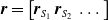
Moreover, a VSR can be equipped with sensors, that are located in its voxels. At each time step, the output of a sensor S, that is, the sensor reading, is $\boldsymbol{{r}}_S \in [0,1]^m$ , where m is the dimensionality of the sensor type. Here, we employ four types of sensors, which provide the VSR with information about its state and about the surrounding environment:

• Sensors of type area perceive the ratio between the current area of the voxel and its rest area ( $m=1$ ).

• Sensors of type touch sense if the voxel is in contact with the ground or not and output a value being 1 or 0, respectively ( $m=1$ ).

• Sensors of type velocity perceive the velocity of the center of mass of the voxel along the x- and y-axes ( $m=2$ ) of voxel itself.

• Sensors of type vision perceive the distance towards close objects, as the terrain or any obstacle, within some field of view, i.e., along a set of directions. For each direction, the corresponding element of the sensor reading $\boldsymbol{{r}}_S$ is the distance of the closest object, if any, from the voxel center of mass of the voxel along that direction. If the distance is greater than a threshold d, it is clipped to d. We use the vision sensor with the following directions with respect to the voxel positive x-axis: $-\dfrac{1}{4} \pi$ , $-\dfrac{1}{8} \pi$ , 0, $\dfrac{1}{8} \pi$ , $\dfrac{1}{4} \pi$ ; the dimensionality is hence $m=5$ .

Velocity and vision sensors employ a soft normalization of the outputs, using, respectively, the $\tanh$ function and rescaling, to ensure that the output is defined in $[0,1]^m$ .

3.2 VSR controller

The VSR controller is, in general, a parametric multivariate function, $f_{\boldsymbol{\theta}}$ , which computes the actuation value for each voxel given some inputs, for example, the sensor readings, at every simulation time step. Given a morphology and a parametric function, a VSR can be optimized for a given task by optimizing the controller parameters $\boldsymbol{\theta}$ .

In this study, we experiment with two architectures of neural controllers, that is, controllers based on ANNs, taking inspiration from (Talamini et al., Reference Talamini, Medvet, Bartoli and De Lorenzo2019) and (Medvet et al., Reference Medvet, Bartoli, De Lorenzo and Seriani2020).

3.2.1 Centralized neural controller

The first controller architecture we experiment with is the one proposed by Talamini et al. (Reference Talamini, Medvet, Bartoli and De Lorenzo2019). The controller function $f_{\boldsymbol{\theta}}$ is implemented by a fully connected feedforward ANN, also known as multilayer perceptron, where the number of input neurons corresponds to the overall number of sensor readings, and the number of outputs corresponds to the number of voxels in the VSR.

At each time step, this controller processes the concatenation $\boldsymbol{{r}}=\left[\boldsymbol{{r}}_{S_1} \; \boldsymbol{{r}}_{S_2} \; \dots \right]$ of the current sensor readings and uses its output $\boldsymbol{{a}} \in [\!-1,1]^n = f_{\boldsymbol{\theta}}(\boldsymbol{{r}})$ as actuation values for the n voxels composing the VSR. We use $\tanh$ as the activation function in the neurons of the ANN.

We call this variant a centralized controller as there is a single central ANN processing the sensory information coming from each voxel to compute all the actuation values of the VSR.

The centralized controller parameters coincide with the synaptic weights of the ANN, $\boldsymbol{\theta} \in \mathbb{R}^p$ , with p depending on the ANN topology, that is, the number and size of the ANN layers—we recall that the size of the input and output layers are determined by the sensors the VSR is equipped with and the number of voxels, respectively.

A schematic representation of a centralized controller for a simple VSR composed of three voxels is shown in Figure 2. In this example, each voxel is equipped with two sensors and the ANN has one hidden layer consisting of 5 neurons. As a result, this centralized controllers has $p=|\boldsymbol{\theta}|= (6+1) \cdot 5 + (5+1) \cdot 3=53$ parameters, the $+1$ being associated with the bias.

Figure 2. A schematic representation of the centralized controller for a $3 \times 1$ VSR with two sensors in each voxel. Blue and red curved arrows represent the connection of the ANN with inputs (sensors) and outputs (actuators), respectively.

3.2.2 Distributed neural controller

The second controller architecture we consider is the distributed controller developed by Medvet et al. (Reference Medvet, Bartoli, De Lorenzo and Seriani2020) to exploit the intrinsic modularity of VSRs. The key idea is that each voxel is equipped with an ANN, which processes local inputs to produce the actuation value for said voxel. Hence $f_{\boldsymbol{\theta}}$ is the ensemble of the functions $f^i_{\boldsymbol{\theta}_i}$ implemented by each ANN. In order to enable the transfer of information along the body of the VSR, neighboring voxels are connected by means of $n_c$ communication channels. Namely, each ANN reads the sensors values together with the $4 n_c$ values coming from adjacent voxels, and in turn outputs an actuation signal and $4 n_c$ values to feed to contiguous voxels. Note that this controller architecture results in an overall recurrent ANN, which is responsible for introducing an additional dynamics to the one deriving from the mechanical model of the VSR.

More in detail, each ANN takes as input a vector $ \boldsymbol{{x}}^i = \left[ \boldsymbol{{r}}_S^i \ \boldsymbol{{i}}_{N} \ \boldsymbol{{i}}_{E} \ \boldsymbol{{i}}_{S} \ \boldsymbol{{i}}_{W} \right]$ where $\boldsymbol{{r}}_S^i$ are the local sensor readings, and $\boldsymbol{{i}}_{N}^i$ , $\boldsymbol{{i}}_{E}^i$ , $\boldsymbol{{i}}_{S}^i$ , $\boldsymbol{{i}}_{W}^i$ (each one $\in \mathbb{R}^{n_c}$ ) are the input communication values coming from the adjacent voxel placed above, right, below, left—if the voxel is not connected to another voxel on a given side, the corresponding vector of communication values is the zero vector $\textbf{0} \in \mathbb{R}^{n_c}$ . Each ANN outputs a vector $\boldsymbol{{y}}^i = f^i_{\boldsymbol{\theta}_i}\left(\boldsymbol{{x}}^i\right) = \left[ a \ \boldsymbol{{o}}_{N}^i \ \boldsymbol{{o}}_{E}^i \ \boldsymbol{{o}}_{S}^i \ \boldsymbol{{o}}_{W}^i\right]$ where a is the local actuation value, and $\boldsymbol{{o}}_{N}^i$ , $\boldsymbol{{o}}_{E}^i$ , $\boldsymbol{{o}}_{S}^i$ , $\boldsymbol{{o}}_{W}^i$ are the vectors of $n_c$ output communication values going towards the adjacent voxel placed above, right, below, left of the voxel.

Figure 3 shows a scheme of a distributed neural controller for a $3\times1$ VSR.

Figure 3. A schematic representation of the distributed controller for a $3\times1$ VSR with two sensors in each voxel and $n_c=1$ communication channel per side. Blue and red curved arrows represent the connection of the ANN with inputs (sensors and input communication channels) and outputs (actuator and output communication channels), respectively.

Output communication values produced by the ANN of a voxel at time step $k-1$ are used by the adjacent voxels ANNs at k, which introduces some delay in the propagation of signals across the VSR body. Not only could such propagation delay be beneficial, as shown by Cheney et al. (Reference Cheney, Clune and Lipson2014), but it also has a biological foundation (Segev and Schneidman, Reference Segev and Schneidman1999).

Concerning the controller parameters, they consist of the concatenation of the parameters of each voxel ANN: 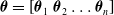$\boldsymbol{\theta}=\left[ \boldsymbol{\theta}_1 \ \boldsymbol{\theta}_2 \dots \boldsymbol{\theta}_n \right]$ , where n is the number of voxels composing the VSR.

The distributed controller in a VSR can be instantiated according to two design choices: (a) there could be an identical ANN in each voxel, both in terms of architecture and weights (homo-distributed), or (b) each voxel can have its own independent ANN that can differ from others in weights, hidden layers, and number of inputs and outputs (hetero-distributed). The main differences between the two proposed configurations regard the optimization process and the allowed sensor equipment of the VSRs. Namely, for a VSR controlled by a homo-distributed controller, each voxel needs to have the same amount of sensor readings to pass to the controller, to ensure the number of inputs fed to the ANN is the same. In addition, evolving a single ANN for each voxel requires less exploration, given the reduced number of parameters to optimize (all $\boldsymbol{\theta}_i$ are the same), but likely requires more fine-tuning to make it adequate for controlling each voxel and achieve a good global performance. On the contrary, the hetero-distributed architecture leaves more freedom, allowing any sensor configuration, but has a much larger search space in terms of number of parameters to optimize.

The distributed neural controllers for VSRs used in this work have a similarity with neural cellular automata (NCA) techniques (Nichele et al., Reference Nichele, Ose, Risi and Tufte2017; Mordvintsev et al., Reference Mordvintsev, Randazzo, Niklasson and Levin2020), in which the lookup table of each cellular automaton (CA) cell is replaced by an ANN. The ANN therefore defines the cell next state by processing the local information of its nearest neighbors. NCA have been successfully used to grow and replicate CA shapes and structures with neuroevolution (Nichele et al., Reference Nichele, Ose, Risi and Tufte2017) and with differentiable learning (Mordvintsev et al., Reference Mordvintsev, Randazzo, Niklasson and Levin2020), to produce self-organising textures (Niklasson et al., Reference Niklasson, Mordvintsev, Randazzo and Levin2021), to grow 3D artifacts (Sudhakaran et al., Reference Sudhakaran, Grbic, Li, Katona, Najarro, Glanois and Risi2021), for regenerating soft robots (Horibe et al., Reference Horibe, Walker and Risi2021), and for controlling reinforcement learning agents (Variengien et al., Reference Variengien, Nichele, Glover and Pontes-Filho2021).

5.1 Characterization of pruning variants in static and disembodied conditions

We aimed at evaluating the effect of different forms of pruning on ANNs in terms of how the output changes with respect to no pruning, given the same input. In order to make this evaluation significant with respect to the use case of this study, that is, ANNs employed as controllers for VSRs, we considered ANNs with topologies that resemble the ones used in the next experiments and fed them with inputs that resemble the readings of the sensors of a VSR doing locomotion.

In particular, for the ANN topology we considered three input sizes $n_{\textrm{input}} \in \{10,25,50\}$ and three depths $n_{\textrm{layers}} \in \{0,1,2\}$ , resulting in $3 \cdot 3 = 9$ topologies, all with a single output neuron. For the topologies with inner layers, we set the inner layer size to the size of the input layer. In terms of the dimensionality p of the vector $\boldsymbol{\theta}$ of the parameters of the ANN, the considered ANN topologies correspond to values ranging from $p=(10+1) \cdot 1=11$ , for $n_{\textrm{input}}=10$ and $n_{\textrm{layers}}=0$ , to $p=(50+1) \cdot (50+1) \cdot (50+1) \cdot 1 = 132\, 651$ , for $n_{\textrm{input}}=50$ and $n_{\textrm{layers}}=2$ , where the $+1$ is the bias. We instantiated 10 ANNs for each topology, setting $\boldsymbol{\theta}$ by sampling the multivariate uniform distribution $U(\!-1,1)^p$ of appropriate size, hence obtaining 90 ANNs.

Concerning the input, we fed the network with sinusoidal signals with different frequencies for each input, discretized in time with a time step of $\Delta t = {1/10}\ \mathrm{s}$ . Precisely, at each time step k, with $t=k\Delta t$ , we set the ANN input to $\boldsymbol{{x}}^{(k)}$ , with $x_i^{(k)} = \sin\left(\frac{k\Delta t}{i+1}\right)$ , and we read the single output $y^{(k)}=f_{\boldsymbol{\theta}}\left(\boldsymbol{{x}}^{(k)}\right)$ .

We considered the $3 \cdot 5$ pruning variants (scope and criteria) and 20 values for the pruning rate $\rho$ , evenly distributed in $[0,0.75]$ . We took each one of the 90 ANNs and each one of the 300 pruning variants, we applied the periodic input for 10 s, triggering the actual pruning at $t_p= 5\ \mathrm{s}$ , and we measured the mean absolute difference e between the output $f_{\boldsymbol{\theta}}\left(\boldsymbol{{x}}^{(k)}\right)$ during the last 5 s, that is, after pruning, and the output $f_{\hat{\boldsymbol{\theta}}}\left(\boldsymbol{{x}}^{(k)}\right)$ of the corresponding unpruned ANN:

(1) \begin{equation} e=\frac{1}{50}\sum_{k=50}^{k=100} \left\lVert f_{\boldsymbol{\theta}}\left(\boldsymbol{{x}}^{(k)}\right)-f_{\hat{\boldsymbol{\theta}}}\left(\boldsymbol{{x}}^{(k)}\right)\right\rVert.\end{equation}

Figure 4 summarizes the outcome of this experiment. It displays one plot for each ANN topology (i.e., combination of $n_{\textrm{layer}}$ and $n_{\textrm{input}}$ ) and one line showing the mean absolute difference e, averaged across the 10 ANNs with that topology, vs. the pruning rate $\rho$ for each pruning variant: the color of the line represents the criterion, the line type represents the context. Larger ANNs are shown in the bottom right of the matrix of plots.

Figure 4. Mean absolute difference e between the output of a pruned ANN and the output of the corresponding unpruned ANN vs. the pruning rate $\rho$ , for different ANN structures and with different pruning criteria (color) and scopes (linetype).

By looking at Figure 4, we can do the following observations. First, the factor that appears to have the largest impact on the output of the pruned ANN is the criterion (the color of the line in Figure 4). Weight and absolute signal mean criteria consistently result in lower values for the difference e, regardless of the scope and the pruning rate. On the other hand, with the signal mean criterion, e becomes large even with low pruning rates: for $\rho>0.1$ there seems to be no further increase in e. Interestingly, the random criterion appears to be less detrimental, in terms of e, than signal mean in the vast majority of cases. We explain this finding by the kind of input these ANNs have been fed with, that is, sinusoidal signals: the mean of periodic signals with a period shorter enough than the time before pruning is close to 0 and this results in connections actually carrying some information to be pruned. We recall that we chose to use sinusoidal signals because they are representative of the sensor readings a VSR doing locomotion could collect, in particular when exhibiting an effective gait, that likely consists of movements that are repeated over the time.

Second, apparently, there are no bold differences among the three values for the scope parameter. As expected, for the shallow ANNs (with $n_{\textrm{layers}}=0$ ), the scope parameter does not play any role, since there is one single layer and one single output neuron (being the same destination for all connections).

Third, the pruning rate $\rho$ impacts on e as expected: in general, the larger $\rho$ , the larger e. However, the way e changes by increasing $\rho$ seems to depend on the pruning criterion: for weight and absolute signal mean, Figure 4 suggests a linear dependency. For the other criteria, e quickly increases with $\rho$ and then remains stable, for signal mean, or increases more slowly, for signal variance and random.

Fourth and finally, the ANN topology appears to play a minor role in determining the impact of pruning. The ANN depth (i.e., $n_{\textrm{layers}}$ ) seems to impact slightly on the difference between pruning variants: the deeper the ANN, the fuzzier the difference. Concerning the number of inputs $n_{\textrm{input}}$ , by looking at Figure 4 we are not able to make any strong claim.

Based on the results of this experiment, summarized in Figure 4, we decided to consider only weight, absolute signal mean, and random criteria and only the network scope for the next experiments.

To better understand the actual impact of the chosen pruning variants on the output $y^{(k)}$ of an ANN, we show in Figure 5 the case of two ANNs. The figure shows the value of the output of the unpruned ANN (in gray), when fed with the input described above (up to $t= 20 \mathrm{s}$ ), and the outputs of the $3 \cdot 4$ pruned versions of the same ANN, according to the three chosen criteria and four values of $\rho$ .

Figure 5. Comparison of the output of pruned and unpruned versions of two ANNs of different structures: $n_{\mathrm{input}}=10$ , $n_{\mathrm{layers}}=0$ , above, and $n_{\mathrm{input}}=100$ , $n_{\mathrm{layers}}=2$ , below. Pruning occurs at $t_p= 5\ \mathrm{s}$ .

5.2 RQ1: impact on the evolution

In order to understand if the evolution of VSR controllers is hindered by pruning, we performed various experiments.

First, we evaluated the effect of pruning on different controller architectures and ANN topologies. To this extent, we evolved nine VSR controllers, resulting from the combination of three architectures and three ANN topologies, and one morphology.

We experimented with the three controller architectures presented in Section 3.2: centralized, homo-distributed, and hetero-distributed. We combined each of these with different ANN topologies, considering ANNs with $n_{\textrm{layers}} \in \{0,1,2\}$ . For the ANNs with hidden layers, we set the size of those layers to match the size of the input layer. Regarding the distributed controllers, we set $n_c=2$ , and for the hetero-distributed architecture we kept the amount of hidden layers homogeneous throughout the entire VSR.

Concerning the VSR morphology, we employed the biped, which consists of 10 voxels arranged in a $4\times 3$ grid, as shown in Figure 1a. We experimented with two different sensor configurations: uniform, where each voxel is equipped with velocity, touch, and area sensors; and spined-touch-sighted, with area sensors in each voxel, velocity sensors in the voxels in the top row, touch sensors in the voxels in the bottom row, and vision sensors in the voxels of the rightmost column. These two configurations resulted in 40 and 35 overall sensor readings, respectively.

We combined the spined-touch-sighted configuration with the centralized and the hetero-distributed controller architectures, whereas we used the uniform configuration in conjunction with the homo-distributed architecture due to its requirements of having the same amount of sensors in each voxel. Table 1 summarizes the number of parameters to be optimized for each VSR controller we evolved.

Table 1. Number of parameters to be optimized by the EA for each controller architecture and ANN topology

For each of the nine combinations of controller architecture and ANN topology, we used three different pruning criteria: weight, absolute signal mean, and random, all with network scope, as thoroughly described in Section 4. For each criterion, we employed the following pruning rates: $\rho \in \{0.125, 0.25, 0.5, 0.75\}$ . We remark that for distributed controllers, we applied pruning separately for each voxel ANN. Furthermore, we evolved, for each combination, a controller without pruning to have a baseline for meaningful comparisons.

To perform evolution, we used the simple evolutionary algorithm (EA) described in Algorithm 2, a form of evolutionary strategy. At first, $n_{\textrm{pop}}$ individuals, that is, numerical vectors $\boldsymbol{\theta}$ , are put in the initially empty population, all generated by assigning to each element of the vector a value sampled from the uniform distribution $U(\!-1,1)$ . Subsequently, $n_{\textrm{gen}}$ evolutionary iterations are performed. On every iteration, which corresponds to a generation, the fittest quarter of the population is chosen to generate $n_{\textrm{pop}}-1$ children, each obtained by adding values sampled from a normal distribution $N(0,\sigma)$ to each element of the element-wise mean $\boldsymbol{\mu}$ of all parents. The generated offspring, together with the fittest individual of the previous generation, end up forming the population of the next generation, which maintains the fixed size $n_{\textrm{pop}}$ .

We used the following EA parameters: $n_{\textrm{pop}}=48$ , $n_{\textrm{gen}}= 416$ (corresponding to 20 000 fitness evaluations), and $\sigma=0.35$ . We verified that, with these values, evolution was in general capable of converging to a solution, that is, longer evolutions would have resulted in negligible fitness improvements.

We optimized VSRs for the task of locomotion: the goal of the VSR is to travel as fast as possible on a terrain along the positive x-axis. We quantified the degree of achievement of the locomotion task of a VSR by performing a simulation of duration $t_f$ and measuring the VSR average velocity 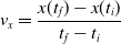$v_x=\dfrac{x(t_f)-x(t_i)}{t_f-t_i}$ , x(t) being the position of the robot center of mass at time t and $t_i$ being the initial time of assessment. In the EA of Algorithm 2, we hence used $v_x$ as fitness for selecting the best individuals. We set $t_f= 60\ \mathrm{s}$ and $t_i= 20\ \mathrm{s}$ to discard the initial transitory phase. For the controllers with pruning, we set the pruning time at $t_p= 20\ \mathrm{s}$ : this way the evaluation of the fitness of the VSR only takes into consideration the velocity after pruning. In section Section 5.4, instead, we investigate the effects of determining the VSR fitness considering both the pre- and the post-pruning velocities ( $t_i<t_p$ ).

We remark that the EA of Algorithm 2 constitutes a form of Darwinian evolution with respect to pruning: the effect of pruning on an individual does not impact on the genetic material that is passed to the offspring by that individual. More precisely, the element-wise mean $\boldsymbol{\mu}$ is computed by considering the parents $\boldsymbol{\theta}$ vectors before the pruning.

For favoring generalization, we evaluated each VSR on a different randomly generated hilly terrain, that is, a terrain with hills of variable heights and distances between each other. To avoid propagating VSRs that were fortunate in the random generation of the terrain, we re-evaluated, on a new terrain, the fittest individual of each generation before moving it to the population of the next generation.

For each of the $3 \cdot 3 \cdot (3 \cdot 4 + 1)$ combinations of controller architecture, ANN topology, pruning criterion, and pruning rate (the $+1$ being associated with no pruning), we performed 10 independent, that is, based on different random seeds, evolutionary optimizations of the controller with the aforementioned EA. We hence performed a total of 1170 evolutionary optimizations. We used 2D-VSR-Sim (Medvet et al., Reference Medvet, Bartoli, De Lorenzo and Seriani2020) for the simulation, setting all parameters to default values.

5.2.1 Impact of the controller architecture and the ANN topology

Figure 6 summarizes the findings of this experiment. In particular, the plots show how the pruning rate $\rho$ impacts the fitness of the best individual of the last generation, for the different controller architectures and ANN topologies employed in the experiment.

Figure 6. Fitness $v_x$ (median with lower and upper quartiles across the 10 repetitions) vs. pruning rate $\rho$ , for different pruning criteria (color), controller architectures (plot row), and ANN topologies(plot column).

The most remarkable trait of the plots is that individuals whose controllers have been pruned with weight or absolute signal mean criteria significantly outperform those who have undergone random pruning. This suggests that randomly pruning controllers at each fitness evaluation is detrimental to their evolution. In fact, individuals with a good genotype could perform poorly after the removal of important connections, while others could surpass them thanks to a luckier pruning, hence the choice of fittest individuals for survival and reproduction could be distorted. Moreover, Figure 6 confirms that the heuristics employed, based on weight and absolute signal mean criteria (Section 4), successfully choose connections that are less important for the controller to be removed, thus limiting the damage of connection removal.

In addition, comparing the subplots of Figure 6, there are no bold differences between the rows, which leads us to conclude that the architecture of the controller does not play a key role in determining the impact of pruning on the performance of the controller.

Similarly, different ANN topologies are not affected much diversely by pruning, as we notice no sharp distinctions between the columns of the plots. The first subplot, however, stands out from the others, as the trend of the lines seems to suggest that for the centralized controller architecture with no hidden layers pruning could have a beneficial effect. However, the upper and lower quartiles reveal that the distribution of the fitness $v_x$ is spread across a considerably large interval, hence it is difficult to draw any sharp conclusion on the possible benefits of pruning for such controller.

For all other subplots, we can note that a higher pruning rate $\rho$ leads to weaker performance of the controller. In this case, the result is in line with expectations, as an increasing $\rho$ means that we are removing more connections from the ANN, thus reducing its expressiveness. Nevertheless, controllers pruned with a proper heuristic have evolved to achieve results comparable to those who have not undergone pruning during their evolution, considered here as baseline. We performed a Mann–Whitney U test with the null hypothesis that, for each combination of controller architecture, ANN topology, pruning criterion, and pruning rate $\rho$ , the distribution of the best fitness is the same as obtained from the corresponding baseline controller, that is, with the same controller architecture and ANN topology, evolved without pruning, and we found that the p-value is greater than $0.05$ in 66 out of 108 cases.

5.2.2 Impact of the VSR morphology

Having noticed no significant difference between the centralized and distributed controller architectures, we decided to assess the impact of pruning on different VSR morphologies using only the centralized controller architecture. To do so, we performed the evolutionary optimization of three additional VSRs, combining the three ANN topologies employed in the previous experiment with the wormmorphology.

Such morphology consists of 10 voxels arranged in a $5\times2$ grid, as displayed in Figure 1b. We equipped the VSR with the spined-touch-sighted sensor configuration, similarly to what we have done in the previous experiment with the centralized controller architecture and the biped morphology. The amount of parameters to be optimized is the same as in the first column of Table 1, as the two VSR morphologies share the same amount of voxels and sensor readings, hence the number of inputs and outputs of the controller ANNs is the same in both cases.

We repeated the exact experimental pipeline as before, employing the same pruning criteria and pruning rates, without changing any hyper-parameter. For each of the $3\cdot(3\cdot4+1)$ combinations of ANN topology, pruning criterion, and pruning rate, we performed 10 independent evolutionary optimizations, for a total of 390 runs.

The results are displayed in Figure 7, together with the outcomes of the previous experiment for the centralized controller architecture for the biped morphology. The conclusions we can draw from this matrix of plots are rather similar to what we have observed for Figure 6, both in terms of pruning criteria and in terms of differences among the various ANN topologies employed. We can assess the effect of pruning on different VSR morphologies by comparing the rows of the figure, deducing that the biped and the worm are impacted in a substantially equal manner by pruning.

Figure 7. Fitness $v_x$ (median with lower and upper quartiles across the 10 repetitions) vs. pruning rate $\rho$ , for different pruning criteria (color), VSR morphologies (plot row), and ANN topologies (plot column).

As before, controllers pruned with a proper heuristic achieve results comparable to those who have not undergone pruning during their evolution. To confirm this, we performed a Mann–Whitney U test with the null hypothesis that, for each combination of VSR morphology, ANN topology, pruning criterion, and pruning rate $\rho$ , the distribution of the best fitness is the same as obtained from the corresponding baseline controller, that is, with the same VSR morphology and ANN topology, evolved without pruning, and we found that the p-value is greater than $0.05$ in 30 out of 72 cases.

5.2.3 Pruning after the evolution

Based on the results of Figure 6 and Figure 7, we speculate that controllers pruned with weight and absolute signal mean criteria look robust to pruning because they result from an evolution in which VSRs are subjected to pruning, rather than because those kinds of pruning are, per se, not particularly detrimental. To test this hypothesis, we carried out an additional experiment. We took the best individuals of the last generations for the centralized controller with the biped morphology and we re-assessed them (on a randomly generated hilly terrain similar to the one used in evolution). For the individuals that were evolved without pruning, we performed $3\cdot 4$ additional evaluations, introducing pruning after $t_p= 20\ \mathrm{s}$ with the previously mentioned 3 criteria and 4 rates $\rho$ .

Figure 8 shows the outcome of this experiment, that is, $v_x$ on the re-assessment plotted against the re-assessment pruning rate $\rho$ for both individuals evolved with (solid line) and without (dashed line) pruning. The foremost finding is that individuals who evolved with pruning visibly outperform the ones whose ancestors have not experienced pruning, for almost all pruning rates. This corroborates the explanation we provided above, that is, VSRs whose ancestors evolved experiencing pruning are more robust to pruning than VSRs that evolved without pruning.

Figure 8. Median, lower quartiles, and upper quartiles of re-assessment velocity $v_x$ vs. re-assessment pruning rate $\rho$ of individuals evolved with and without pruning for different ANN topologies for the centralized controller and biped morphology.

Besides analyzing the aggregate results, we also examined the behavior of a few evolved VSRs in a comparative way, that is, with and without pruning in re-assessment. We found that, interestingly, in some cases the VSR starts to move effectively only after pruning: this might suggest that pruning shaped the evolutionary path at the point that the lack of pruning becomes detrimental, similarly to what happens in the brain of complex animals (see Section 2). We provide videos of a few VSRs exhibiting a change in their behavior after pruning at https://youtu.be/-HCHDEb9azY, https://youtu.be/oOtJKri6vyw, and https://youtu.be/uwrtNezTrx8. We speculate that choosing $t_i=t_p$ might be a contributing cause to this neat behavioral shift, hence in Section 5.4 we investigate the effects of setting $t_i<t_p$ .

5.3 RQ2: impact on the adaptability

For the sake of this research question, we defined VSR controllers as adaptable if they are able to effectively accomplish locomotion on terrains that none of their ancestors ever experienced locomotion on. Hence, to assess the adaptability of evolved controllers, we measured the performance in locomotion of the best individuals of the last generations on a set of different terrains. We experimented with the following terrains: (a) flat, (b) hilly with 6 combinations of heights and distances between hills, (c) steppy with 6 combinations of steps heights and widths, (d) downhill with 2 different inclinations, and (e) uphill with 2 different inclinations (Figure 9). As a result, each individual was re-assessed on a total of 17 different terrains. Note that, in this experiment, controllers were not altered in between evolution and re-assessment, i.e., they were re-evaluated with the same pruning criterion, if any, and pruning rate $\rho$ as experienced during evolution.

Figure 9. Different types of terrains employed for measuring VSR adaptability.

Figure 10 displays the outcome of this experiment. Namely, for each of the different controller architectures, VSR morphologies, ANN topologies, and pruning criteria, the re-assessment velocity $v_x$ (averaged on the 17 terrains) is plotted against the pruning rate $\rho$ . The results in Figure 10 are coherent with the findings of Section 5.2: comparing the subplots, we can conclude that neither the controller architecture nor the morphology of the VSR are relevant in determining the effect of pruning on adaptability, whereas the ANN topology is somewhat of impact. More in details, for shallow networks, pruning seems to enhance adaptability for the centralized controller architecture, whereas it has a slightly detrimental effect in all other cases.

Figure 10. Median, lower quartiles, and upper quartiles of re-assessment velocity $v_x$ vs. pruning rate $\rho$ averaged across re-assessment terrains for different pruning criteria, VSR controller architectures, VSR morphologies, and ANN topologies.

Anyway, for controllers evolved employing weight or absolute signal mean pruning criteria, the re-assessment results are comparable to those of controllers evolved without pruning. We performed a Mann-Whitney U test with the null hypothesis that, for each combination of controller architecture, VSR morphology, ANN topology, pruning criterion, and pruning rate $\rho$ , the distribution of the average re-assessment velocities across all terrains is the same as the one obtained from the re-assessment of the corresponding baseline controller, i.e., with the same VSR morphology and ANN topology, evolved without pruning, and we found that the p-value is greater than $0.05$ in 79 out of 144 cases.

5.4 RQ3: life-long effectiveness

In the previous experiments, the behavior of the VSR before the pruning played no role in determining the fitness of the robot, hence in driving the evolution. To determine whether evolution could eventually find a path towards VSR controllers that are life-long effective, we repeated the experimental pipeline described for RQ1, setting $t_i= 5\ \mathrm{s}$ and $t_p= 20 \ \mathrm{s}$ for the velocity $v_x$ calculation—we still “discard” the first 5 s of each simulation to avoid considering transient behaviors. This way, the VSR fitness is computed by taking into account both phases of the life of the VSR, before and after the occurrence of pruning. Such procedure has stronger biological resemblance than discarding the pre-pruning life for fitness computation, as in nature the survival and mating likelihoods are estimated on the entire lifespan of an individual, and not only after full brain development.

Since for RQ1 and RQ2 we have noticed no significant differences between the different controller architectures, VSR morphologies, and ANN topologies, for this analysis we only experiment with the centralized controller architecture with an ANN with one hidden layer on the biped morphology. Again, we perform 10 independent evolutionary optimizations, each based on a different random seed.

Figure 11 displays the results for this experiment (right plot), paired with those obtained with the corresponding configuration for RQ1 (left plot). Namely, for each pruning criterion, the median and the quartiles of velocity at the end of evolution $v_x$ are plotted against the pruning rate. Observing the plots, we can answer affirmatively to RQ3: evolution has indeed managed to find a successful path towards controllers that can perform effectively both before and after pruning. Comparing the two plots of Figure 11, there are no outstanding differences, so we can draw similar conclusions as for RQ1, in the sense that pruning remains not significantly detrimental, provided that it is applied with proper heuristics and not randomly.

Figure 11. Fitness $v_x$ (median with lower and upper quartiles across the10 repetitions) vs. pruning rate $\rho$ , for controllers evolved with $t_i=t_p=20 \ \mathrm{s}$ (first column) and controllers evolved with $t_i=5\ \mathrm{s}$ and $t_p=20\ \mathrm{s}$ (second column). Both controllers share the centralized architecture, the ANN topology with $n_{\textrm{layers}}=1$ , and the biped morphology.

To gain further insights, we considered the velocity of the evolved VSRs separately for the two phases of life (before and after pruning). More in detail, we computed the pre-pruning velocity using $t_i=5\ \mathrm{s}$ and $t_f=20\ \mathrm{s}$ and the post-pruning velocity with $t_i=20\ \mathrm{s}$ and $t_f=60\ \mathrm{s}$ . The results are shown in Figure 12, where, similarly as before, the measured velocity is plotted against the pruning rate for each pruning criterion applied. In the plots, the solid line indicates the pre-pruning velocities, while the dashed line represents the post-pruning velocities. Comparing the two lines for each criterion, we can note that for the weight and absolute signal mean criteria, there is a small gap between the two lines, which indicates that most of the controllers abilities are retained after pruning. Contrarily, for the random criterion, there is a significant performance decrease after the occurrence of pruning, which is in line with the previous findings (Section 5.2). We explain this result as follows: since random pruning acts differently on individuals of the same evolutionary lineage, evolution is not able to “guarantee” good performance after pruning. However, since it is also driven by the performance before pruning, evolution produces controllers that are effective in terms of prepruning velocity. Put simply, with random pruning, only one of the two objective in a biobjective evolutionary optimization is actually improvable.

Figure 12. Median, lower quartiles, and upper quartiles of velocity $v_x$ vs. pruning rate $\rho$ of individuals before (solid line) and after (dashed line) pruning for different pruning criteria (color).

Having observed that, similarly to biological organisms, controllers can evolve to be effective both before and after pruning, we decided to investigate the performance of such controllers also in terms of adaptability. To this extent, we repeated the experimental pipeline described for RQ2.

Figure 13 shows the re-assessment velocities for this experiment (right plot), paired with those obtained with the corresponding configuration for RQ2 (left plot). From the comparison of the two subplots, individuals that were evolved in a more biologically plausible fashion, that is, taking into account both the pre- and postpruning velocities for fitness evaluation, seem to be slightly more adaptable than those whose evolution was carried out considering only the post pruning performance. However, the difference between the two plots is not significant, hence we cannot draw sharp conclusions on this.

Figure 13. Average re-assessment velocity $v_x$ (median with lower and upper quartiles across the 10 repetitions) vs. pruning rate $\rho$ , for controllers evolved with $t_i=t_p=20\ \mathrm{s}$ (first column) and controllers evolved with $t_i=5\ \mathrm{s}$ and $t_p=20 \ \mathrm{s}$ (second column). Both controllers share the centralized architecture, the ANN topology with $n_{\textrm{layers}}=1$ , and the biped morphology.

5.5 VSR behavior analysis

Having observed that pruning does not significantly affect the velocities of VSRs in locomotion, we decided to investigate its behavioral impact. Namely, we aimed at systematically evaluating whether the pre- and post-pruning behaviors of VSRs were substantially different. To this extent, we relied on a consolidated data analysis procedure consisting of 1. feature extraction, 2. dimensionality reduction, and 3. visualization.

The features we employed to capture a VSR behavior in locomotion (Medvet et al., Reference Medvet, Bartoli, Pigozzi and Rochelli2021) are based on the movement of the center of mass of the VSR over time and on the way the VSR touches the ground during gait, i.e., its footprints. Here we provide just a brief description of the feature extraction procedure—we refer the reader to (Medvet et al., Reference Medvet, Bartoli, Pigozzi and Rochelli2021) for further details.

Concerning the center of mass movement, we extracted its signals on the x- and y-axis from a sequence H of snapshots—a snapshot is the description of the spatial configuration of every voxel of the VSR at a given time step—and we computed the signals of their first differences. From these, we calculated the Fast Fourier Transforms (FFT), from which we took the magnitude and we filtered out frequency components not in the range $[0\ \mathrm{Hz}, 10\ \mathrm{Hz}]$ . Last, we re-sampled the obtained signals to have $n_{\textrm{freq}}=100$ components for each axis, constituting the final feature vector related to the center of mass movement.

Regarding the footprints, for each snapshot at each time step k, we projected the minimal bounding square of the VSR on the x-axis, that is, the smallest square parallel to the x-axis that completely contains the VSR, and we partitioned the projection in 8 equal sections, from which we built a binary vector (of size 8), the footprint, where each element was set to 1 iff the VSR was touching the ground for more than half of the corresponding segment. To extract some features from the footprints, we considered a sequence of snapshots H, which we processed in the following way:

1. 1. We split H in a sequence of non-overlapping subsequences, each corresponding to $\Delta t_{\textrm{footprint}}= 0.5\ \mathrm{s}$ .

2. 2. We computed the sequence M of footprints, where each element was obtained as the element-wise mode of the footprints in the corresponding subsequence;

3. 3. We considered all the non-overlapping n-grams of footprints in M, $2\leq n\leq 10$ occurring at least twice, we computed their overall duration and we selected the main n-gram $M^\star$ as the one with the longest overall duration.

4. 4. We processed $M^\star$ to obtain the following descriptors: average touch area of the footprints in $M^\star$ , overall duration of all $M^\star$ occurrences, length of the main n-gram $|M^\star|$ , mode of the intervals between consecutive occurrences of $M^\star$ , and rate of intervals that are equal to the mode.

We obtained the feature vector related to the footprints of the VSR through the concatenation of the features extracted from $M^\star$ .

Given the concatenation of the feature vectors of the center of mass movement and of the footprints, we performed dimensionality reduction using the principal component analysis (PCA) from 25 to 2 components, in order to visualize the results in scatter plots.

We exploited the aforementioned analysis pipeline to evaluate the impact of pruning on the behavior of a VSR. In addition, we investigated whether changing the beginning evaluation time $t_i$ with respect to the pruning time $t_p$ would result in more or less visible behavioral differences. To this extent, we focused on the VSR configuration we employed both in RQ1 and RQ3, namely, the biped morphology with the centralized controller architecture with an ANN with 1 hidden layer.

For each evolved VSR, we extracted the behavior features in a re-assessment performed on flat terrain, in order to minimize the impact of any terrain irregularities on the features. To distinguish pre- and post-pruning behaviors, we performed the feature extraction on two separate intervals of the VSR lifetime: before pruning, from $5\ \mathrm{s}$ to $20\ \mathrm{s}$ , and after pruning, from $20\ \mathrm{s}$ to $60\ \mathrm{s}$ .

The results are shown in the scatter plots of Figure 14 and Figure 15, for VSRs evolved with $t_i=t_p= 20\ \mathrm{s}$ (i.e., with the evolution driven only by post-pruning performance) and $t_i= 5\ \mathrm{s}$ and $t_p= 20\ \mathrm{s}$ (i.e., with the evolution driven by life-long performance), respectively. Each point in the scatter plot corresponds to a behavior defined by the aforementioned features, its size depends on the velocity achieved by the VSR in the evaluation interval.

Figure 14. Scatter plots of the first two components resulting from the PCA analysis of the features described in Section 5.5 for the biped VSR with a centralized controller. Each subplot corresponds to a pruning criterion (row) and a pruning rate $\rho$ (column); pruning is applied at $t_p=t_i=20\ \mathrm{s}$ . The color of the bubble indicates whether the evaluation of velocity and feature extraction were performed before or after the occurrence of pruning, while the size of the bubble is proportional to the achievedvelocity $v_x$ .

Figure 15. Scatter plots of the first two components resulting from the PCA analysis of the features described in Section 5.5 for the biped VSR with a centralized controller. Each subplot corresponds to a pruning criterion (row) and a pruning rate $\rho$ (column); pruning is applied at $t_p=20\ \mathrm{s}$ ( $t_i=5\ \mathrm{s}$ ). The color of the bubble indicates whether the evaluation of velocity and feature extraction were performed before or after the occurrence of pruning, while the size of the bubble is proportional to the achieved velocity $v_x$ .

Comparing the two figures, the most outstanding trait is that in Figure 14 the distributions of behaviors achieved after pruning seem to detach more from the pre pruning behaviors distributions, compared to Figure 15, where the two distributions show in general a greater overlap—this difference is particularly visible for small pruning rates. To give an explanation to this result, we recall that the VSRs of Figure 14 have been evolved with $t_i=t_p=20\ \mathrm{s}$ , hence the evaluation of fitness does not consider the prepruning behavior of the robot. We hypothesize that in these circumstances evolution pushes the VSR towards a reasonable postpruning behavior, but does not incentive prepruning effectiveness. Therefore, we can notice a significant shift between the pre- and postpruning behaviors. Contrarily, VSRs of Figure 15 have been evolved with $t_i=5\ \mathrm{s}$ , that is, driven by life-long performance. This explains the smaller shift in behaviors, since the VSRs are required to achieve successful locomotion both before and after pruning.

Focusing on Figure 15, it can be seen that for large pruning rates pre- and postpruning distributions seem to diverge more. Nevertheless, there is a small but non negligible behavior shift also for VSRs whose controllers do not undergo pruning (first column, $\rho=0$ ). Moreover, diversity among behaviors of different robots evolved and re-assessed in the same conditions (i.e. markers of the same color in the same plot) is itself quite large. Based on these considerations, we cannot spot any sharp general trend concerning the effect of pruning on the behavior of evolved VSRs.

Concerning the behavioral shifts induced by different pruning criteria, we cannot draw any sharp conclusion from the plots, either. Comparing the rows of Figure 15, we can notice that with $\rho\leq 0.25$ , the greatest deviation is induced by the absolute signal mean criterion, while the VSRs still retain most of their abilities. With a larger pruning rate, instead, the shifts caused by all criteria are comparable, but, while the VSRs pruned with a proper heuristic generally preserve their velocities, the randomly pruned ones suffer from a significant performance decrease.