

1. Introduction
This paper examines the role of monetary policy in mitigating stock market value procyclicality and promoting macroeconomic and financial stability in an economy able to generate stock market bubbles. The literature has brought different views on this matter over the decades. For a long time, the prevailing one was that central banks should abstain from intervening in the presence of stock market bubbles [see Galì (Reference Galì2014)] due to possible unintended consequences and to the difficulty of detecting actual bubble episodes [Bernanke and Gertler (Reference Bernanke and Gertler1999, Reference Bernanke and Gertler2001) and Greenspan (Reference Greenspan2002)]. Price and financial stability were perceived as complementary objectives, and monetary policy should have remained focused on inflation control [Taylor (Reference Taylor2008)], intervening only eventually to “clean up the mess” left by the bubble burst. A new conventional view arose after the 2008 financial crisis, assigning central banks the role of actively acting to curb bubbles by raising interest rates [see, among others, Miao et al. (Reference Miao, Shen and Wang2019) and Allen et al. (Reference Allen, Barlevy and Gale2018)]. This has been labeled the “leaning against the wind” (LAW) policy.
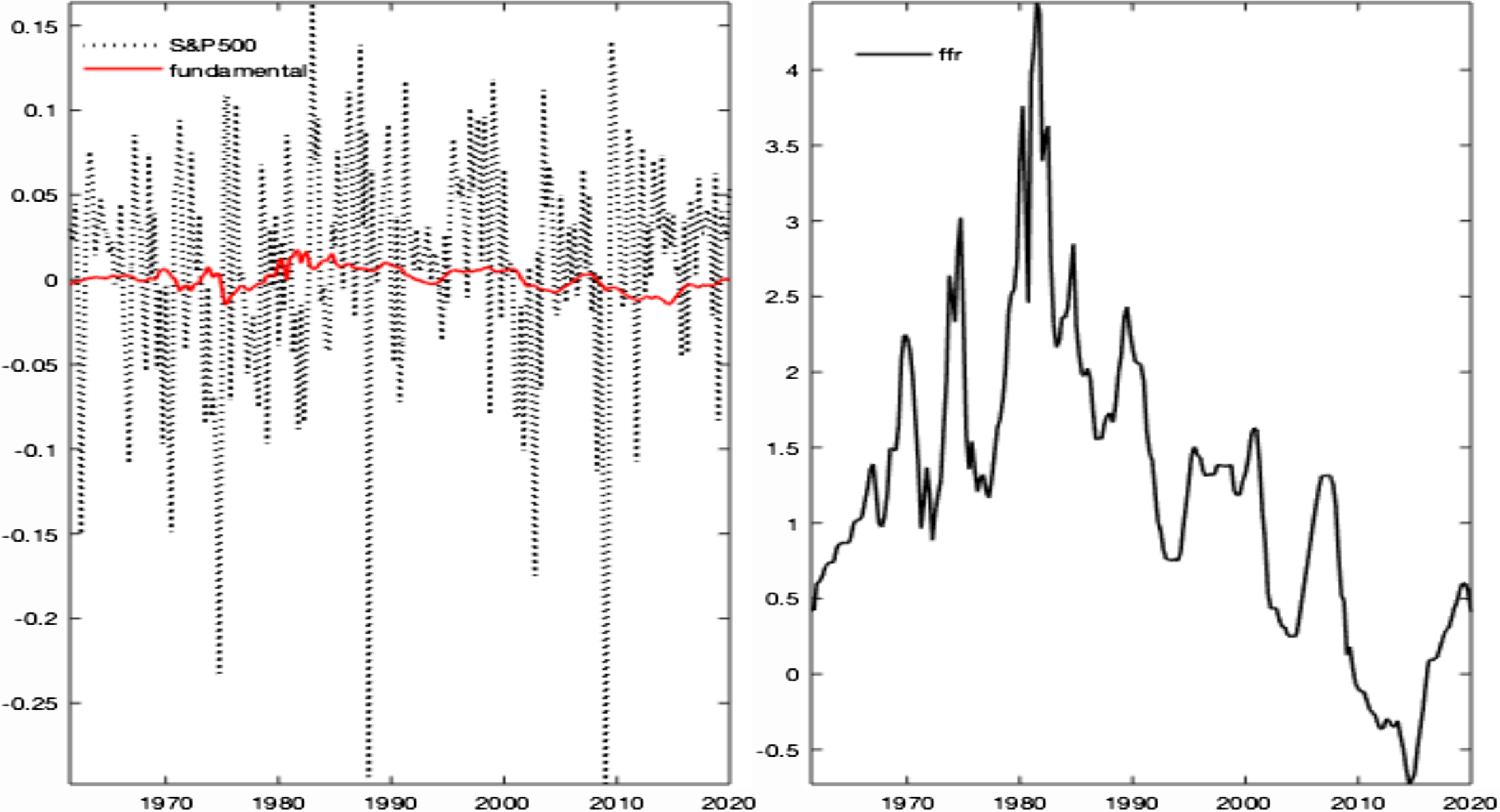
Figure 1. Data evidence: monetary and financial facts. Notes: The left plot shows the time series for the S&P500 stock price (black dotted line), and its fundamental component (red line), namely the present value of future dividend streams. The bubbly component results from the vertical distance between these two series. The right plot depicts the federal funds rate. US sample: 1960–2019.
Notwithstanding the fierce debate over the last decades, the literature on bubbles is still unable to: (i) agree on the effects of monetary policy on bubbles; (ii) assess the relevance of underlying macro-financial conditions to measure policy effectiveness on bubbles’ mitigation; and (iii) rationalize through theoretical channels the related existing evidence.Footnote 1
The aim of this paper is twofold. Since part of the debate builds on an empirical dilemma, we first use a Markov-switching structural vector autoregressive (MS-VAR) to provide new evidence on the effects of monetary policy shocks on asset prices and their bubble component. We consider the joint behavior of asset price and monetary policy cycles [see Corsi and Sornette (Reference Corsi and Sornette2014), Nneji (Reference Nneji2015), Bianchi et al. (Reference Bianchi, Lettau and Ludvigson2022), and Herwartz and Roestel (Reference Herwartz and Roestel2022)], generating monetary-financial regimes for stock market bubbles. Depending on the regime in place, a monetary policy tightening increases stock prices and enhances procyclicality. Then, an OLG model of asset price bubbles is used to study the monetary policy transmission mechanism in an economy with nominal rigidities and collateral-constrained borrowers. Consistently with the MS-VAR, the monetary policy rule is augmented to consider reactions to bubbles and is subject to regime changes jointly with the parameter governing the bubble size. Agents form their expectations based on empirically calibrated transition probabilities. Since their beliefs affect equilibrium outcomes, we perform credibility scenarios to show that policy announcements, agents’ expectations, and learning mechanisms play a crucial role in monetary policy transmission.
Our empirical and model-based findings relate to the long-debated bubble identification and measurement issue. Specifically, a financial bubble is defined as a temporary deviation of a stock price from its fundamental value, namely the present value of future dividend streams [Cochrane (Reference Cochrane2001)]. Using this convention, Figure 1 shows that most asset price fluctuations are described by periodically growing and collapsing bubble episodes, as also reported by the bubbles detection empirical literature [Driffill and Sola (Reference Driffill and Sola1998), Hall et al. (Reference Hall, Psaradakis and Sola1999), Brooks and Katsaris (Reference Brooks and Katsaris2005), Michaelides et al. (Reference Michaelides, Tsionasb and Konstantakis2016), and Chan and Santi (Reference Chan and Santi2021)]. However, this definition runs into the objection raised by Fama (Reference Fama1991)’s joint hypothesis problem, which questions the ability to reliably detect and evaluate asset price bubbles.Footnote 2 We address this criticism in light of Greenwood et al. (Reference Greenwood, Shleifer and You2019), showing that sharp increases in asset prices, while not necessarily predicting low future returns, can predict a heightened probability of a subsequent crash. As long as specific characteristics of acute price rises can help identify future asset price bubbles, monetary authorities may use empirically relevant theoretical models to inform data-driven policy making, considering asset price bubbles within the target variables.
Under these premises, we first empirically test the low-frequency relationship among monetary policy, bubbles, and asset prices by estimating a MS-SVAR on US 1960–2019 data. We characterize model dynamics by using data for real output, real dividends, output and commodity inflation, the federal funds rate, and the real stock price index. A standard recursive scheme identifies the model. We then select the regime-switching specification from a set of nonlinear candidate models. The optimal one, nonlinear in the interest rate and the stock price MS-VAR equations, is able to detect, date, and estimate bubbly regimes generated by the interaction of the monetary and financial dynamics.
The empirical analysis shows that recurrent regimes in the monetary and financial environment determine the effectiveness of monetary policy on asset prices. First, we extract recurrent regimes which align with historical monetary policy changes and financial deepening events. On this basis, we label the states in the stochastic model component as variance states, generating high, medium, and low shocks’ size, and those in the systematic component as monetary-financial states, generating regimes of “high” and “low finance”. The former emerge as periods with higher asset prices, equity returns, and real interest rates. Higher premia generate and inflate bubbles, whose size is, in turn, conditionally higher.
Second, state-dependent impulse responses show that a monetary tightening may be ineffective in reducing stock prices, further inflating their bubble component. This is more relevant in the high finance regime, when bubbles exist and are large, showing that the conditional stock price dynamics depend on the relative size of the bubble. Under the high finance regime, monetary policy tightening generates persistent increases in nominal and real interest rates, thus more sharply affecting output and real dividends. Deeper recession/deflation combines with a positive response of the stock price bubble component, which, when dominant over the fundamental component, is responsible for increased asset prices in the long run.
Equipped with this evidence, we present an OLG model incorporating financial frictions and capturing the interaction between monetary policy and bubble dynamics. We adopt a Markov-switching version of the model for bubbles presented in Ciccarone et al. (Reference Ciccarone, Giuli and Marchetti2019), which, in line with Galì (Reference Galì2014), Martin and Ventura (Reference Martin and Ventura2016), is rooted in a well-established tradition of models of macroeconomic equilibria under rational bubbles. They stem from the seminal work of Tirole (Reference Tirole1985) and Weil (Reference Weil1987).Footnote 3 Our model includes borrowers and lenders in the credit market, physical capital accumulation, and financial frictions. These credit market imperfections constrain the borrowing capacity of investors in productive capital to the collateral value they can pledge. Nominal frictions in the formation of final goods’ prices are also included and provide a role for monetary policy in fixing the nominal interest rate. Furthermore, bequests from old borrowers to young borrowers make it possible to adopt a realistic numerical version of the model.
In line with the MS-VAR evidence, Markov-switching nonlinearities [Farmer et al. (Reference Farmer, Waggoner and Zha2009)] affect the bubble size and the monetary policy rule.Footnote 4 Model calibration is obtained by matching the model- and VAR-based regime-dependent impulse responses, given the estimated transition probabilities. The calibration generates a first regime corresponding to the high finance MS-VAR state, where agents invest in bubbles, monetary policy is more persistent and less reactive to inflation but more reactive to the bubble. Under this regime, the bubble level can weaken the effect of financial frictions, allowing borrowers to demand more funds.Footnote 5 The calibration also generates a regime corresponding to the low finance VAR state, with no bubbles, stronger responsiveness to inflation, and lower interest rate persistence.
The model’s predictions align with the empirical evidence and suggest that a monetary tightening is ineffective in reducing stock prices and inflates bubbles, especially in a high finance regime. This pro-cyclical effect operates through the increase in the real interest rate, which, in addition to the demand channel favoring future consumption, generates two different results: (i) a reduction in the demand for credit through the price channel (increased cost of borrowed funds); (ii) an increase in the aggregate savings’ share allocated to non-productive assets, displacing investments from productive capital, through allocation channel. These recessive channels more than compensate for the expansionary effect of the increase in the bubble size through the collateral channel. Moreover, a bubbly regime of magnified recession/deflation is explained by the augmented regime-dependent monetary policy rule: following the exogenous increase in the policy rate, the increase in the real rate, driven by the fall in inflation, is partially offset by the central bank’s reaction to the increased bubble component. This result produces a more substantial persistence in the nominal interest rate response, higher real rates, and a more severe recession/deflation.
Agent’s expectations play a crucial role in this mechanism. We assess the role of announcements’ credibility by building scenarios where agents attach different probabilities to the occurrence of a regime change. We show that the credibility of announcing a different policy can significantly affect the efficacy of the current policy stance. For instance, in response to an announced shift toward a stabilizing regime (low finance) with no bubble creation, agents start disinvesting in the bubbly asset in anticipation, effectively raising the probability of switching to the no bubble scenario. Alternatively, if agents believe that the transition to a bubbly regime is more likely, a monetary shock’s effect is exacerbated by deeper recession/deflation and bubble inflation.
At last, since our analysis inherently assumes full information with respect to bubble identification and timing, we build counterfactual scenarios to test our results and evaluate the possibility that agents may face uncertainty about the duration of regimes, hence about the emergence of a bubble. We model this behavior as a learning mechanism, where agents cannot precisely infer whether the bubbles are a short- or long-lasting phenomenon [Bianchi et al. (Reference Bianchi, Lettau and Ludvigson2022)]. Investors’ learning leads to a gradual adjustment in the bubble valuation after the regime shift dates, until explaining an overreaction of the bubble to the monetary impulse once learning is complete. Hence, our results are confirmed even when agents face uncertainty about the bubble.
Moreover, if we assume no monetary policy response to the bubble, the recessionary/deflationary effects of a tightening would be dampened. Noteworthy, the theoretical framework adopted in the paper could be, in fact, envisioned as favorable to the LAW policies: we assume that the central banker has sufficient information to detect and—at least partially—evaluate a reference value (in steady state) for the bubble. Even in this favorable analytical framework, the risk of injecting additional instability into the economy would be substantial. This risk is particularly evident in the high finance regime. We interpret this result as offering an additional cautionary argument for central bank activism in contrasting (presumably) pathological bubbly episodes. Nevertheless, we acknowledge that the validity and generality of our main results are limited to the hypotheses specifying the measurability of a bubble, i.e., the evaluation of the fundamental component in asset prices out of other sources of variability (e.g., risk premium, noise, and market frictions).
The paper is structured as follows. In Section 2, we present the empirical strategy. We then discuss the emerging regimes and results from stochastic simulations. Section 3 describes the theoretical model, the monetary policy transmission channels, the policy credibility, and uncertainty scenarios. Section 4 concludes.
2. Empirical evidence
The empirical analysis considers a nonlinear multivariate time series model, specified as a MS-SVAR [Sims and Zha (Reference Sims and Zha2006) and Sims et al. (Reference Sims, Waggoner and Zha2008)], where we identify monetary policy shocks using a standard recursive strategy. Following Galì and Gambetti (Reference Galì and Gambetti2015), we derive the asset price bubble component as the difference between observed (real) stock prices and their fundamental component. The empirical novelty of our study relies on deriving bubbly regimes from the interplay between monetary and financial dynamics.Footnote 6 Then, by simulating a monetary policy tightening, we characterize the uneven transmission dynamics to asset prices—and to its bubble component—over different monetary-financial regimes.
2.1. Bubble derivation
Since Tirole (Reference Tirole1985), a bubble is defined as the difference between the asset price and its fundamental value, as follows:
 \begin{equation*}Q_t^B=Q_t-Q^F_t\end{equation*}
where $Q_t$
denotes the price of an infinite-lived asset,
$Q_t$
denotes the price of an infinite-lived asset, $Q_t^B$
and
$Q_t^B$
and $Q^F_t$
its bubbly and fundamental components.
$Q^F_t$
its bubbly and fundamental components.
A model for the asset fundamental value is required to test for the existence of bubbles.Footnote 7 We rely on the theory of rational asset price bubbles in a discrete-time setting [Giglio et al. (Reference Giglio, Maggiori and Stroebel2016)], such that a rational bubble is assumed to originate from the failure of the transversality condition in the rational asset pricing equation for stocks. According to this theory, a rational bubble grows at the real interest rate:
 \begin{equation*}Q^B_t=E_t\left (\frac {Q^B_{t+1}}{R_t}\right )\end{equation*}
where $R_t$
is the real interest rate factor. This result implies that the price behavior is explosive. The bubble tests developed by Diba and Grossman (Reference Diba and Grossman1988), Hall et al. (Reference Hall, Psaradakis and Sola1999), and Phillips et al. (Reference Phillips, Shi and Yu2015a, Reference Phillips, Shi and Yub) (among others), indeed, ascertain the existence of bubbles from the explosive dynamics in long time series of asset prices, by using unit root and cointegration analysis on the price-dividend relationship. Other approaches, instead, rely on the present-value literature—initiated by Campbell and Shiller (Reference Campbell and Shiller1988) and followed by many others [Balke and Wohar (Reference Balke and Wohar2009), Al-Anaswah and Wilfling (Reference Al-Anaswah and Wilfling2011), and Chan and Santi (Reference Chan and Santi2021)]—for which the fundamental price component is derived under risk neutrality as the present discounted value of future dividend flows [Cochrane (Reference Cochrane2001)], as follows:
$R_t$
is the real interest rate factor. This result implies that the price behavior is explosive. The bubble tests developed by Diba and Grossman (Reference Diba and Grossman1988), Hall et al. (Reference Hall, Psaradakis and Sola1999), and Phillips et al. (Reference Phillips, Shi and Yu2015a, Reference Phillips, Shi and Yub) (among others), indeed, ascertain the existence of bubbles from the explosive dynamics in long time series of asset prices, by using unit root and cointegration analysis on the price-dividend relationship. Other approaches, instead, rely on the present-value literature—initiated by Campbell and Shiller (Reference Campbell and Shiller1988) and followed by many others [Balke and Wohar (Reference Balke and Wohar2009), Al-Anaswah and Wilfling (Reference Al-Anaswah and Wilfling2011), and Chan and Santi (Reference Chan and Santi2021)]—for which the fundamental price component is derived under risk neutrality as the present discounted value of future dividend flows [Cochrane (Reference Cochrane2001)], as follows:
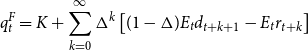 \begin{equation*}q_t^F=K+\sum _{k=0}^{\infty }\Delta ^k\left[(1-\Delta )E_t d_{t+k+1}-E_t r_{t+k}\right]\end{equation*}
where $d_t$
is the dividend stream of the asset price,
$d_t$
is the dividend stream of the asset price, $K=\log (1+Q/D)-\frac{Q/D}{1+Q/D}$
is a constant (where
$K=\log (1+Q/D)-\frac{Q/D}{1+Q/D}$
is a constant (where $Q/D$
the average price-dividend ratio), and
$Q/D$
the average price-dividend ratio), and $\Delta \lt 1$
is the mean difference between the gross rate of growth of dividends and the real rate.
$\Delta \lt 1$
is the mean difference between the gross rate of growth of dividends and the real rate.
We follow Galì and Gambetti (Reference Galì and Gambetti2015) for the derivation of the predicted response of the fundamental component of asset prices to an exogenous shock in the monetary policy rate $\epsilon ^m$
:
$\epsilon ^m$
:
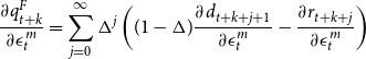 \begin{equation*}\frac {\partial q^F_{t+k}}{\partial \epsilon ^m_t}=\sum _{j=0}^{\infty } \Delta ^j\left ((1-\Delta )\frac {\partial d_{t+k+j+1}}{\partial \epsilon ^m_t}-\frac {\partial r_{t+k+j}}{\partial \epsilon ^m_t}\right )\end{equation*}
such that the response of the bubble component, $\partial q_t^B/\partial \epsilon ^m_t$
, is obtained as the asset price residual
$\partial q_t^B/\partial \epsilon ^m_t$
, is obtained as the asset price residual $q^B_t=q_t-q^F_t$
. Hence, the asset price response is defined as a weighted average of the two responses:
$q^B_t=q_t-q^F_t$
. Hence, the asset price response is defined as a weighted average of the two responses:
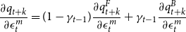 \begin{equation} \frac{\partial q_{t+k}}{\partial \epsilon ^m_t}=(1-\gamma _{t-1})\frac{\partial q_{t+k}^F}{\partial \epsilon ^m_t}+\gamma _{t-1}\frac{\partial q^B_{t+k}}{\partial \epsilon ^m_t} \end{equation}
where the weight $\gamma _t\equiv Q_t^B/Q_t$
denotes the share of the bubble in the observed price. The fundamental component contributes more to the asset price response in periods where its share in asset prices is lower and vice-versa when bubbles are dominant.
$\gamma _t\equiv Q_t^B/Q_t$
denotes the share of the bubble in the observed price. The fundamental component contributes more to the asset price response in periods where its share in asset prices is lower and vice-versa when bubbles are dominant.
A standard literature critique of the bubble theory is that risk attitudes can still explain the residual asset price component once discounted dividends are accounted for. These attitudes are reflected in risk premia, namely the covariance term between the stochastic discount factor and future payoffs. Two features of our approach mitigate this issue. First, we focus our analysis on rational bubbles, which impose restrictions on the dynamics of the bubble component. Second, we use a less restrictive model for fundamentals by allowing the whole asset price equation to switch across regimes—hence, also its fundamental component. Therefore, as argued in Chan and Santi (Reference Chan and Santi2021), the latter also embodies the role of time-varying discount rates and other latent factors driving regimes in fundamentals. Consequently, the residual—namely, our measure for the bubble—is orthogonal to asset price fundamentals and to factors generating shifts in fundamentals.Footnote 8
In Appendix D, we directly tackle this critique by allowing for a risk premium in the decomposition of the asset price response to the monetary shocks, as from the argument by Galì and Gambetti (Reference Galì and Gambetti2015). From this decomposition, the bubble is thus a residual risk premia component as in Jarrow and Lamichhane (Reference Jarrow and Lamichhane2022). We show that accounting for an endogenous response of the equity premium to monetary policy shocks tends to emphasize our primary evidence favoring a positive bubble response.
2.2. The MS-SVAR
The MS-SVAR is estimated with Bayesian methods using quarterly US data spanning from 1960 to 2019. Six variables are included in the model: the real GDP level $y_{t}$
, real dividends
$y_{t}$
, real dividends $d_{t}$
, the GDP inflation rate
$d_{t}$
, the GDP inflation rate $\pi _{t}^{y}$
, the inflation rate for non-energy commodities
$\pi _{t}^{y}$
, the inflation rate for non-energy commodities $\pi _{t}^{c}$
, the federal funds rate
$\pi _{t}^{c}$
, the federal funds rate $r_{t}$
, and the real S&P500 index
$r_{t}$
, and the real S&P500 index $q_{t}$
. All variables enter in logs except for inflation and policy rates. For the latter, we use the shadow interest rate by Wu and Xia (Reference Wu and Xia2016) over the 2009–2016 time interval, in order to consider the zero lower bound period.Footnote
9
$q_{t}$
. All variables enter in logs except for inflation and policy rates. For the latter, we use the shadow interest rate by Wu and Xia (Reference Wu and Xia2016) over the 2009–2016 time interval, in order to consider the zero lower bound period.Footnote
9
Nonlinear dynamics are introduced as Markov-switching state-dependency in the systematic and the stochastic model components. Hence, a Markov chain driving discrete coefficient states, $\xi _t^c$
, controls the former, whereas an independent Markov chain,
$\xi _t^c$
, controls the former, whereas an independent Markov chain, $\xi _t^v$
, controls the latter, capturing discrete states for shocks’ heteroskedasticity. The two chains are collected under a composite process
$\xi _t^v$
, controls the latter, capturing discrete states for shocks’ heteroskedasticity. The two chains are collected under a composite process $\xi _t=\{\xi _t^c, \xi _t^v\}$
, evolving according to the transition matrix
$\xi _t=\{\xi _t^c, \xi _t^v\}$
, evolving according to the transition matrix $Q=Q^{c}\otimes Q^{v}=(q_{i,j})_{(i,j)\in (H\times H)}\in \Re ^{h^{2}}$
, where
$Q=Q^{c}\otimes Q^{v}=(q_{i,j})_{(i,j)\in (H\times H)}\in \Re ^{h^{2}}$
, where $q_{i,j}$
is the transition probability from state
$q_{i,j}$
is the transition probability from state $i$
to state
$i$
to state $j$
and
$j$
and $H=\{1\ldots h\}$
is the set of possible regimes for
$H=\{1\ldots h\}$
is the set of possible regimes for $\xi _{t}$
.Footnote
10
$\xi _{t}$
.Footnote
10
The MS-SVAR model is as follows:
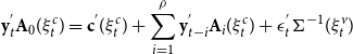 \begin{equation} \mathbf{y}_{t}^{^{\prime }}\mathbf{A}_{0}(\xi _{t}^{c})=\mathbf{c}^{^{\prime }}(\xi _{t}^{c})+\sum _{i=1}^{\rho }\mathbf{y}_{t-i}^{^{\prime }}\mathbf{A}_{i}(\xi _{t}^{c})+\mathbf{\epsilon }_{t}^{^{\prime }}\mathbf{\Sigma }^{-1}(\xi _{t}^{v}) \end{equation}
where $\mathbf{y}_{t}^{\prime }=\left [ \begin{array}{c@{\quad}c@{\quad}c@{\quad}c@{\quad}c@{\quad}c} y_{t} & d_{t} & \pi _{t}^{y} & \pi _{t}^{c} & r_{t} & q_{t}\end{array}\right ]$
,
$\mathbf{y}_{t}^{\prime }=\left [ \begin{array}{c@{\quad}c@{\quad}c@{\quad}c@{\quad}c@{\quad}c} y_{t} & d_{t} & \pi _{t}^{y} & \pi _{t}^{c} & r_{t} & q_{t}\end{array}\right ]$
, $\mathbf{c}(\xi _{t}^{c})$
is the vector of constants,
$\mathbf{c}(\xi _{t}^{c})$
is the vector of constants, $\mathbf{A}_{0}(\xi _{t}^{c})$
is the invertible contemporaneous correlations matrix,
$\mathbf{A}_{0}(\xi _{t}^{c})$
is the invertible contemporaneous correlations matrix, $\mathbf{A}_{i}(\xi _{t}^{c})$
denotes the dynamic cross-correlation matrices for each lag term
$\mathbf{A}_{i}(\xi _{t}^{c})$
denotes the dynamic cross-correlation matrices for each lag term $\rho$
, and
$\rho$
, and $\mathbf{\Sigma }$
is a diagonal matrix capturing structural shocks’ sizes. Following the standard practice in MS-VAR modeling [Sims and Zha (Reference Sims and Zha2006) and Sims et al. (Reference Sims, Waggoner and Zha2008)], we fix
$\mathbf{\Sigma }$
is a diagonal matrix capturing structural shocks’ sizes. Following the standard practice in MS-VAR modeling [Sims and Zha (Reference Sims and Zha2006) and Sims et al. (Reference Sims, Waggoner and Zha2008)], we fix $\rho =5$
(i.e., to the data frequency plus one), and adopt Litterman (Reference Litterman1986)’s random walk prior, consistently with the stochastic properties of the variables.Footnote
11
The calibration of priors follows Sims et al. (Reference Sims, Waggoner and Zha2008), which provide a benchmark for quarterly data MS-SVARs.Footnote
12
A multivariate normal distribution for the orthogonal structural shocks
$\rho =5$
(i.e., to the data frequency plus one), and adopt Litterman (Reference Litterman1986)’s random walk prior, consistently with the stochastic properties of the variables.Footnote
11
The calibration of priors follows Sims et al. (Reference Sims, Waggoner and Zha2008), which provide a benchmark for quarterly data MS-SVARs.Footnote
12
A multivariate normal distribution for the orthogonal structural shocks $\epsilon _{t}$
is assumed:
$\epsilon _{t}$
is assumed:
 \begin{equation} P\left(\mathbf{\epsilon }_{t}|\mathbf{Y}^{t-1},\mathbf{\Xi }_{t},\mathbf{\theta },q\right)=\mathcal{N}\left(\mathbf{\epsilon }_{t}|\mathbf{0}_{n},I_{n}\right) \end{equation}
where the structural shocks’ standard deviations are given by the diagonal elements of $\mathbf{\Sigma }^{-1}(\xi _{t}^{v})$
,
$\mathbf{\Sigma }^{-1}(\xi _{t}^{v})$
, $\mathbf{\theta }$
denotes the vector of the model’s structural parameters, and
$\mathbf{\theta }$
denotes the vector of the model’s structural parameters, and $\mathbf{\Xi }_{t}$
and
$\mathbf{\Xi }_{t}$
and $\mathbf{Y}^{t-1}$
collect past information on the latent processes and data, respectively.
$\mathbf{Y}^{t-1}$
collect past information on the latent processes and data, respectively.
In this framework, we identify the monetary policy shock by imposing the (lower triangular) recursive strategy adopted by Galì and Gambetti (Reference Galì and Gambetti2015)—inherited from Christiano et al. (Reference Christiano, Eichenbaum and Evans2005)—where we order the federal funds rate after GDP, dividends, and inflation but before asset prices. Hence, we assume that monetary policy cannot respond contemporaneously to changes in asset prices and is consistent with some other key features: (i) on impact, only stock prices respond contemporaneously to the federal funds rate shock and (ii) monetary policy can react contemporaneously to output, dividends, and inflation changes. In this vein, we rely on an “information-based” identification approach, according to which slow-moving (real sector) variables do not respond contemporaneously to fast-moving (financial sector) ones, embodying a forward-looking component with considerable predictive content for the real economy.
We then test the relevance and nature of regime switches by computing the marginal data density (MDD) over differently specified competing models. As shown in Appendix B, this analysis selects a best-fit model $\left(3\xi ^v2\xi ^c_{r,q}\right)$
with a three-state Markov chain in the stochastic model component (generating variance states) and a two-state Markov chain in the asset price and interest rate systematic model component (generating monetary-financial states). Therefore, we label
$\left(3\xi ^v2\xi ^c_{r,q}\right)$
with a three-state Markov chain in the stochastic model component (generating variance states) and a two-state Markov chain in the asset price and interest rate systematic model component (generating monetary-financial states). Therefore, we label $\xi ^c=\xi ^{mf}$
. The resulting regimes describe a story of state-dependent monetary policy and financial interaction.
$\xi ^c=\xi ^{mf}$
. The resulting regimes describe a story of state-dependent monetary policy and financial interaction.
Table 1. Descriptive statistics of states: moments
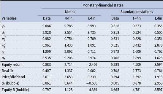
The table reports model variables’ means and standard deviations and some selected derivations, conditional on staying in each state. The equity return is computed as the growth rate of S&P500 stock prices; the real policy rate is the deviation of the federal funds rate from inflation (based on the GDP deflator); “ $q_{t}$
(bubble)” is the bubble component of S&P500 stock prices, as decomposed by Galì and Gambetti (Reference Galì and Gambetti2015), and “Equity return (bubble)” is the return rate of the bubble component of S&P500 stock prices.
$q_{t}$
(bubble)” is the bubble component of S&P500 stock prices, as decomposed by Galì and Gambetti (Reference Galì and Gambetti2015), and “Equity return (bubble)” is the return rate of the bubble component of S&P500 stock prices.
2.3. Monetary-financial regimes
Monetary-financial states reflect nonlinear regularities of structural relations and shocks’ transmission, describing the interaction of monetary and financial phenomena. Their occurrence defines two states: the “high finance state” (H-fin) and the “low finance state” (L-fin). As displayed in Table 1, summarizing some descriptive statistics conditional on states, the former characterizes periods of sustained and stable stock prices and equity returns, higher output, inflation, and higher interest rates; the latter, the low finance state, defines periods of lower stock prices and crushes in equity returns.Footnote 13 By decomposing the S&P500 stock price index in a fundamental and a bubbly component, as explained in Section 2.1, stock prices in the high finance state contain a sizeable bubble component, which explains the higher stock price levels under this regime. Stock returns are also explained (in levels and standard deviations) by their bubble component, which grows at higher and more stable rates. The price-dividend ratio is substantially higher in the high finance regime.
As for the US historical evolution of regimes, Figure 2 reports the smoothed probabilities evaluated at the posterior mode for the Markov chains emerging under the selected model in 1960–2019 quarterly sample. The top panel displays states’ probabilities for the variance, capturing high (dark gray area), medium (light gray area), and low (white area) shocks’ sizes. The bottom panel displays probabilities for the monetary-financial states, where the gray areas identify the high finance state and the white areas the low finance state. The red line tracks the evolution of the monetary policy rate over time to enhance regimes’ interpretation.
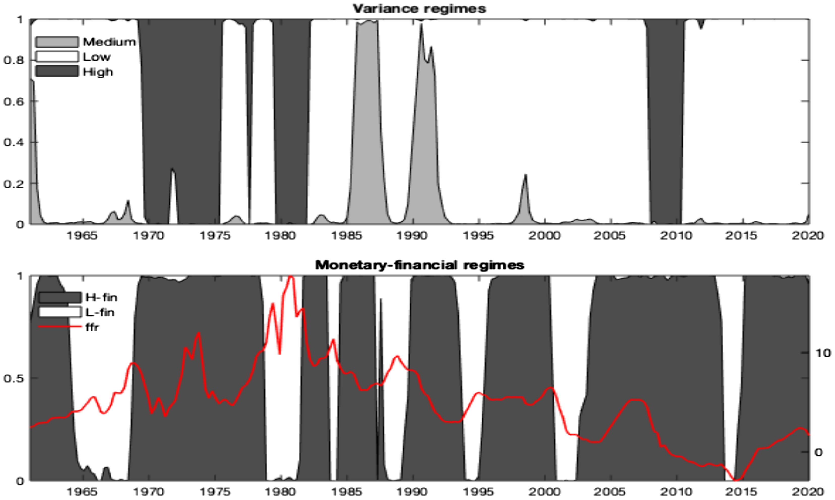
Figure 2. United States: variance and monetary-financial regimes. Notes: The figure shows the states’ smoothed probabilities at the posterior mode from the best-fit benchmark model, $3\xi ^v2\xi ^c_{r,q}$
. The upper plot displays the smoothed probabilities for the variance states. The bottom plot displays the smoothed probabilities for states emerging on the monetary policy and the asset price equations. The series for the interest rate is shown below the latter.
$3\xi ^v2\xi ^c_{r,q}$
. The upper plot displays the smoothed probabilities for the variance states. The bottom plot displays the smoothed probabilities for states emerging on the monetary policy and the asset price equations. The series for the interest rate is shown below the latter.
Variance and coefficient regime switches can be interpreted in terms of historical events. Regimes on shocks’ variances (low, medium, and high) detect high volatility during the two oil price turmoils in the 70s [as in Bianchi and Ilut (Reference Bianchi and Ilut2017)], the reserve targeting period of the early 80s, and the first stages of the global financial crisis in 2008–09. The medium variance regime materialized around the second half of the 80s, covering the stock market crash in 1987 and the recession due to the Gulf War I of the early 90s. The remaining periods, thus the pre-70s, the financial deepening era of the early 90s until 2008, and the post-2009, reflected conditions of relative stability and low variations in shocks (low variance state).
Monetary-financial states emerge as a result of the interaction of monetary and financial phenomena.Footnote 14 Consistent with Jarrow and Kwok (Reference Jarrow and Kwok2021), and Fusari et al. (Reference Fusari, Jarrow and Lamichhanne2022), high finance regimes closely track market performance. In contrast, switches towards low finance states are centered around stock price turning points and occurred in the late 60s, during the first half of the 80s (Volker era), the dot-com bubble (2001), and the 2015–16 stock market sell-off, including the Chinese stock market turbulence, the Greek debt default and the effects of the end of quantitative easing in the US.
2.4. Impulse responses
We evaluate the regime-specific conditional dynamics generated by an unexpected increase in the federal funds rate considering regime-dependent impulse response functions (IRFs).Footnote 15 To enhance the interpretation of results concerning the transmission dynamics across regimes, we condition the IRFs to a 1% contractionary monetary shock in all states.Footnote 16
In Figure 3, impulse responses are regime-dependent and display different channels of monetary transmission, depending on whether the high or low finance state is in place. Specifically, a 1% interest rate shock triggers a drop in real GDP and real dividends, which worsens expectations of future profitability and reduces stock price evaluations, as predicted by the traditional theory.Footnote 17 The high finance state, where the bubbly component of stock prices is higher, features more amplification and less policy effectiveness in stabilizing target variables, leading to more robust and more persistent drops in real activity and dividends and a further increase in real interest rates.
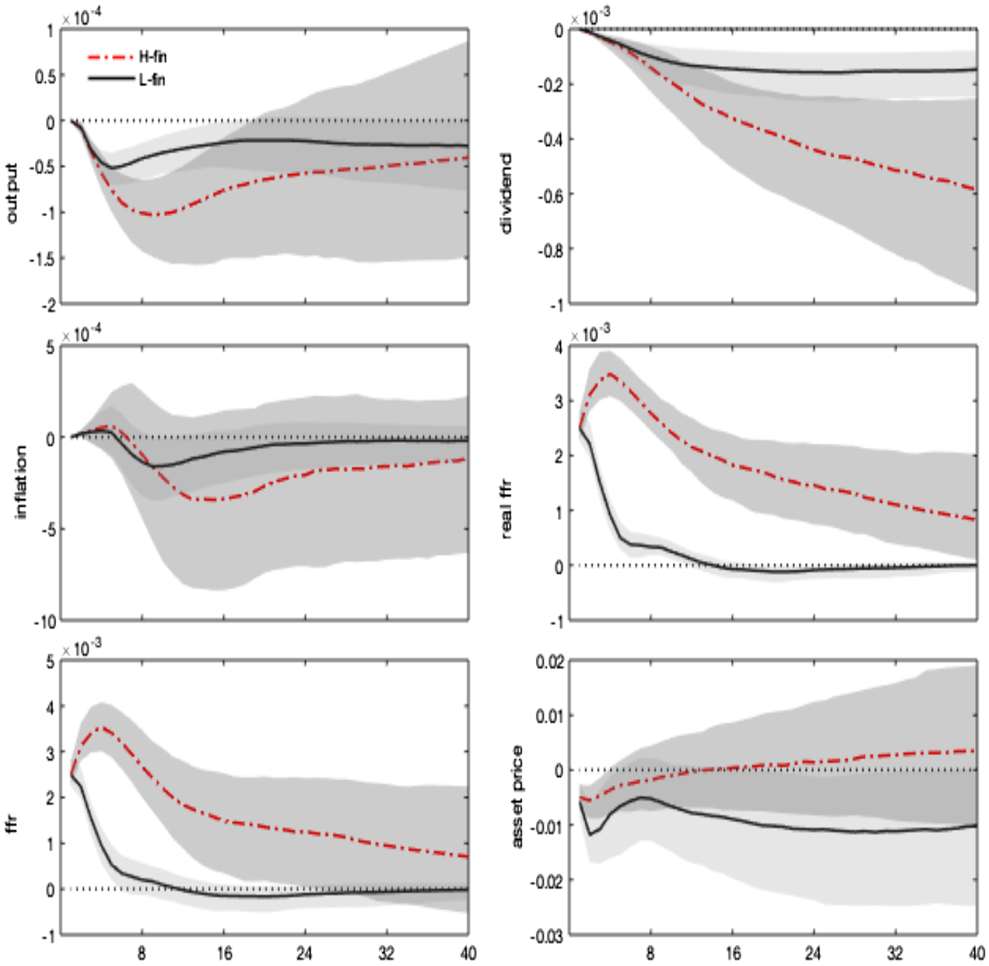
Figure 3. Monetary policy shock. Impulse responses. Notes: The figure shows the impulse responses to a 1% monetary policy shock. The difference across regimes only reflects nonlinearities in the monetary policy and asset price equations, driven by $\xi ^{mf}$
. Shaded areas denote 68% credibility sets.
$\xi ^{mf}$
. Shaded areas denote 68% credibility sets.
Notwithstanding the drop in expected dividends, the fall in stock price is lower under the high finance (bubbly) state and vanishes after 1 year. Indeed, asset prices do not only co-move with dividends but also embed an additional premium resulting from their bubbly component, growing with real rates. By decomposing the stock price impulse response in a fundamental and a bubble component (equation 1), Figure 4 shows that the rise in the real interest rate, combined with the decline in dividends, generates a drop in the asset price fundamental component (in line with the conventional wisdom and economic theory). Under the high finance regime, real rates and dividends respond more, and the bubbly component of asset prices increases. This result is explained by the larger relative size of the bubble, as shown in Table 1, and by the more persistent response of real interest rates.
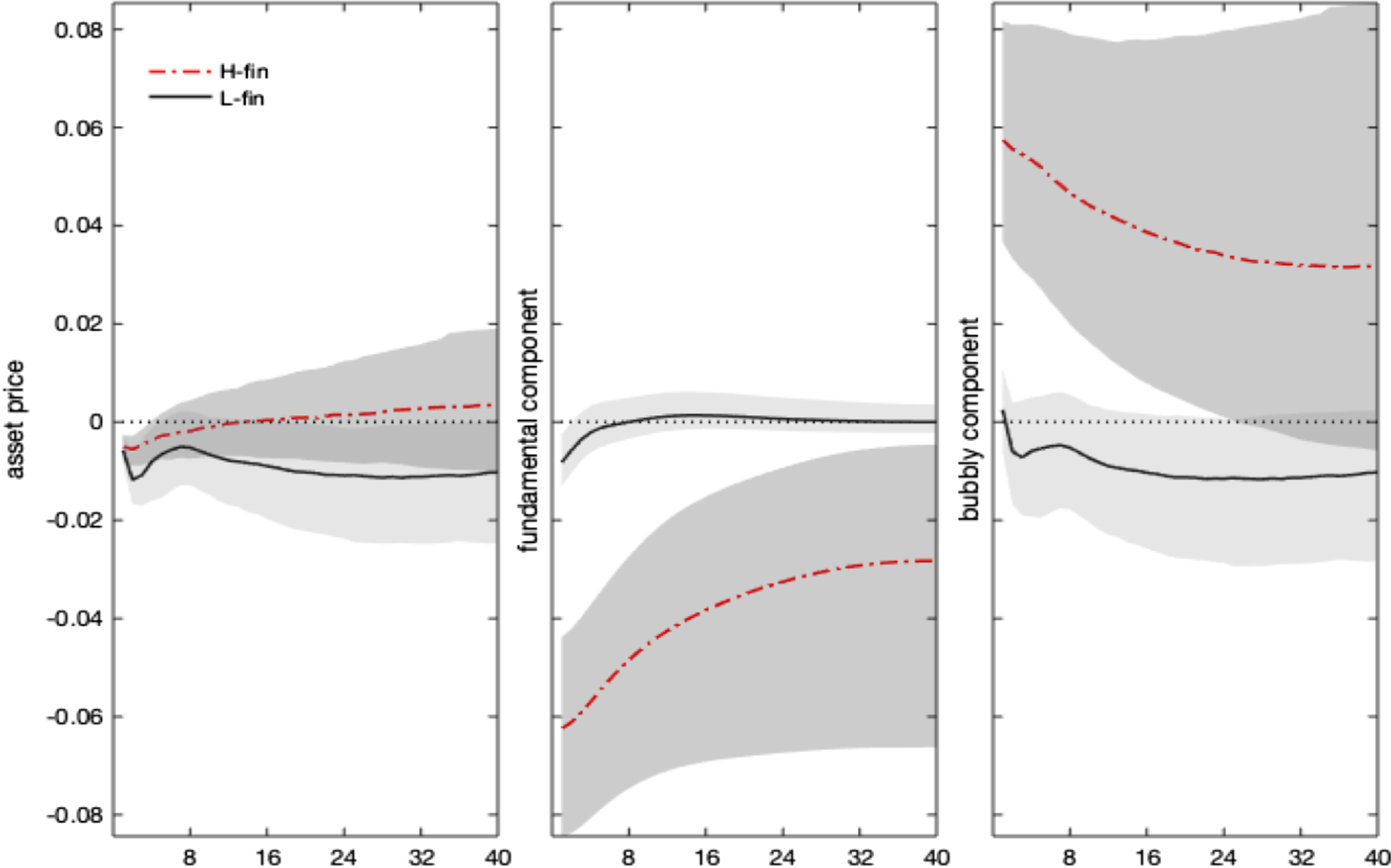
Figure 4. Monetary policy shock. Impulse responses: stock price decomposition. Notes: The figure shows the impulse responses of asset prices, and their decomposition in a fundamental and bubbly component, to a 1% monetary policy shock. Differences across regimes only reflect nonlinearities in the monetary policy and asset price equations, driven by $\xi ^{mf}$
. Shaded areas denote 68% credibility sets.
$\xi ^{mf}$
. Shaded areas denote 68% credibility sets.
Our evidence confirms the findings in Galì and Gambetti (Reference Galì and Gambetti2015), which—using a time-varying VAR—find that an exogenous monetary tightening inflates the bubble, amplifying financial instability, mainly after the 90s with the Great Moderation and the onset of financial deepening. We qualify that heightened monetary-financial interaction, resulting in high equity premia, real rates, and a high bubble share in the composition of asset prices, is the main determinant of their result. Policy ineffectiveness to dampen the emergence of rational bubbles depends on the (recurrent) joint determination of financial outcomes with the monetary policy behavior.
3. A MS-OLG model for bubbles
We introduce Markov-switching behavior in Ciccarone et al. (Reference Ciccarone, Giuli and Marchetti2019)’s analytical model, as described in Appendix G. The economy is populated by overlapping generations (OLG) of agents living for two periods; young and old agents coexist in equal and constant proportion within each period.
The OLG framework is characterized by three main elements: (i) frictional financial markets; (ii) physical capital accumulation; and (iii) sticky prices. Households are grouped in two types: borrowers and lenders in the credit market. Borrowers can invest in physical capital and can trade an additional asset which is modeled as a “pure” bubble, analogous to a pyramid scheme.Footnote 18 Due to asymmetric information between creditors and debtors and the absence of state-contingent securities, the amount of credit that borrowers can obtain varies with the amount of collateral that can be pledged, which also depends on the (expected) value of the bubbly asset.
The economy produces one intermediate good and a continuum of differentiated final goods. Using capital and labor traded in competitive markets, a representative firm produces the intermediate good, which is sold under perfect competition to a continuum of monopolistically competitive final producers. Final goods can be consumed or transformed into new physical capital, and are subject to price stickiness, through which monetary policy displays real effects.
Within each generation, the two classes of agents participate in the final goods market, the markets for productive inputs, and the financial markets. The savers work when young and save part of their labor income to purchase credit contracts paying the nominal interest. The firms producing the final output are owned by the old savers, who pass them on as a bequest at the end of their lives when young savers enter their old age. Profits and interest payments on credit contracts finance the consumption of old savers. Borrowers, who also consume the final good over their lifetime, invest, when young, in the productive (“fundamental”) and in the non-productive (“bubbly”) assets, and finance this expenditure by borrowing in the financial sector and using the resources left to them as a bequest by the borrowers of the previous generation.
Productive investments add to the capital stock, which the young borrowers buy from the old ones at the end of the period. The representative intermediate firm rents physical capital from borrowers and hands them the remuneration of capital when they become old. The bubbly assets are valued on the expectation of their resale value. Each generation of borrowers issues new bubbles with random initial values, which are traded in the market for bubbles alongside the old ones issued by previous generations and sold to the young ones.
In the credit market, identical and perfectly competitive banks accept the deposits demanded by savers and use them to supply the loans demanded by borrowers at the nominal loan rate. At the end of each period, loans and deposits (plus interest) are paid back, banks’ balance sheets clear, and banks shut down to open again at the beginning of the next period. Savers can hold two types of financial assets: money supplied by the central bank and bank deposits. The central bank sets the interest rate on deposits by following a dynamic rule targeting inflation and the bubbly asset.Footnote 19
Old borrowers supply the outstanding bubbles issued in the previous period and can issue new bubbles. Young borrowers demand both types of the bubble. Young savers, who supply labor inelastically, enter each period without previously accumulated cash holdings and deposits, receive money wage income, and deposit at banks. At the end of the period, deposits and interest earnings are repaid. A cash-in-advance constraint requires agents to allocate money balances and money wage income for consumption, net of the deposits they make at banks. The old savers receive the aggregate profits obtained from retailer firms and banks and are not interested in carrying financial assets to the future (bequest motive).
Credit market imperfections affect the behavior of banks, which may not always obtain the full repayment of the loans provided to the borrowers. To obtain loans, borrowers must then provide credit intermediaries with collateral. They can pledge only a fraction of their future resources but create and exchange a bubbly asset that can also be used as collateral. The overall guarantee provided by borrowers eliminates the need for banks to add a risk premium on top of the riskless rate.
The OLG model is Markov-switching in the bubble size and the monetary policy rule, according to a Markov process capturing monetary-financial regimes. This feature generates two states, namely the high finance and low finance states, in line with the empirical evidence. In this modeling framework, agents form expectations knowing that in each period the economy can switch to a different monetary-financial state of the economy, with a given transition probability.
3.1. The market for bubbles
The equilibrium between demand (by young borrowers) and supply (by old borrowers) of the bubble in every period is $B_{t+1}=B_{t}+B_{t+1}^{N}$
, where
$B_{t+1}=B_{t}+B_{t+1}^{N}$
, where $B_{t+1}\geq 0$
is the physical amount of the bubble supplied at
$B_{t+1}\geq 0$
is the physical amount of the bubble supplied at $ t+1$
and
$ t+1$
and $B_{t+1}^{N}$
represents newly issued bubbles. The bubble equilibrium equation can be expressed as
$B_{t+1}^{N}$
represents newly issued bubbles. The bubble equilibrium equation can be expressed as
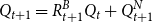 \begin{equation} Q_{t+1}=R_{t+1}^{B}Q_{t}+Q_{t+1}^{N} \end{equation}
where $R_{t+1}^{B}=P_{t+1}^{B}/P_{t}^{B}$
is the real factor of return on the bubble,
$R_{t+1}^{B}=P_{t+1}^{B}/P_{t}^{B}$
is the real factor of return on the bubble, $P_{t+1}^{B}$
and
$P_{t+1}^{B}$
and $Q_{t}=P_{t}^{B}B_{t}$
are the real price and the real value of the bubble, respectively. The new bubble creation process is linked to the economy’s size through the parameter
$Q_{t}=P_{t}^{B}B_{t}$
are the real price and the real value of the bubble, respectively. The new bubble creation process is linked to the economy’s size through the parameter $\omega \gt 0$
:
$\omega \gt 0$
: $q_{t}^{N}=\omega y=\omega Ak^{\alpha }$
, where
$q_{t}^{N}=\omega y=\omega Ak^{\alpha }$
, where $q_{t}^{N}=Q_{t}^{N}/g^t$
is the trend-less value of the new bubble and
$q_{t}^{N}=Q_{t}^{N}/g^t$
is the trend-less value of the new bubble and $y$
,
$y$
, $k$
are the stationary levels of output and capital, respectively; hence,
$k$
are the stationary levels of output and capital, respectively; hence, $\omega$
measures the bubble-to-output ratio.Footnote
20
If
$\omega$
measures the bubble-to-output ratio.Footnote
20
If $\omega =0$
, the economy sets itself into a “no bubble” stationary state in which the level of capital
$\omega =0$
, the economy sets itself into a “no bubble” stationary state in which the level of capital $k_{\text{NB}}$
is generally lower than that of a “bubbly” economy (
$k_{\text{NB}}$
is generally lower than that of a “bubbly” economy ( $\omega \gt 0$
).
$\omega \gt 0$
).
We assume the bubble share follows a two-state Markov process $\xi ^{mf}_t$
, capturing the financial side of the monetary-financial interaction we evidence in the MS-VAR. The Markov process produces two states: a bubbly and a no-bubbly scenario.Footnote
21
The monetary policy counterpart will be discussed in the next section.
$\xi ^{mf}_t$
, capturing the financial side of the monetary-financial interaction we evidence in the MS-VAR. The Markov process produces two states: a bubbly and a no-bubbly scenario.Footnote
21
The monetary policy counterpart will be discussed in the next section.
In order to understand the effects of $\bar{\omega }$
on the stationary value of capital
$\bar{\omega }$
on the stationary value of capital $k$
, and hence on
$k$
, and hence on $y$
, take the equilibrium relationship between
$y$
, take the equilibrium relationship between $k$
and the real interest factor
$k$
and the real interest factor $R$
in the credit market,
$R$
in the credit market, $Ak^{\alpha -1}=f_{B}\left ( R\right )$
from equation (G27), and solve it for
$Ak^{\alpha -1}=f_{B}\left ( R\right )$
from equation (G27), and solve it for $k$
. Then, compute the following derivative:
$k$
. Then, compute the following derivative:
 \begin{align*} \frac {dk(R)}{d\bar {\omega }} & =\frac {gk(R)^{2-\alpha }}{\left ( 1-\alpha \right )AR} \left [ \frac {\phi r^k-\frac {\varepsilon _{R,\bar {\omega }}}{\bar {\omega }}\left ( \frac {r^{k}}{\mu \alpha }\left ( \phi \mu \alpha +\bar {\omega } \right ) +\left ( 1-\delta _{K}\right ) \phi \right ) }{\frac {g}{R}( \phi \mu \alpha +\bar {\omega })} +\frac {\left ( 1-\phi \right ) \eta }{ \eta +\beta }\mu \alpha \right ]\\[4pt] \varepsilon _{R,\bar {\omega } } & =\frac {dR/R}{\frac {d\bar {\omega }}{\bar {\omega }} }\gt 0,\,\,\,\,r^{k}=\alpha \mu Ak^{\alpha -1}\end{align*}
The sign of $\frac{dk\left ( R\right ) }{d\bar{\omega } }$
defines two different regions for the effect on capital of an increase in the bubble share. We are in crowding-in (crowding-out) when an increase (decrease) in the bubble share ends up stimulating (dampening) the accumulation of capital:
$\frac{dk\left ( R\right ) }{d\bar{\omega } }$
defines two different regions for the effect on capital of an increase in the bubble share. We are in crowding-in (crowding-out) when an increase (decrease) in the bubble share ends up stimulating (dampening) the accumulation of capital:
 \begin{equation*} \bar {\omega } \phi r^{k}-\left [ \left ( r^{k}+1-\delta _{K}\right ) \phi +\frac {q^{N}}{k}\right ] \varepsilon _{R,\bar {\omega } }\gtrless 0 \end{equation*}
Therefore, the direction in which the bubble share $\bar{\omega }$
in the (locally unique) stationary state affects capital depends on three different channels acting on the three terms of the above inequality:
$\bar{\omega }$
in the (locally unique) stationary state affects capital depends on three different channels acting on the three terms of the above inequality:
-
Collateral channel: an increase in the bubbly asset (higher $\bar{\omega }$
) slackens the collateral constraint allowing borrowers to demand more funds and invest more. This yields a positive effect on
$k$
and
$y$
(crowding-in), through the term
$\bar{\omega } \phi r^{k}$
;
$\bar{\omega }$
) slackens the collateral constraint allowing borrowers to demand more funds and invest more. This yields a positive effect on
$k$
and
$y$
(crowding-in), through the term
$\bar{\omega } \phi r^{k}$
; -
Price channel: a higher
$\bar{\omega }$
increases the cost of borrowed funds, leading borrowers to demand fewer funds and to invest less. This result produces a negative effect on
$k$
and
$y$
(crowding-out), via the term
$\varepsilon _{R,\bar{\omega }}$
; -
Asset allocation channel: a higher
$\bar{\omega }$
increases the quantity of the bubbly asset to be purchased, crowding out productive investment expenditures. This effect increases with the total return on capital, and it yields a negative effect on
$k$
and
$y$
(crowding-out), through the term
$\left (r^{k}+1-\delta _{K}\right ) \phi +\frac{q^{N}}{k}$
.


The final effect of an exogenous increase of $\bar{\omega }$
on
$\bar{\omega }$
on $k$
(i.e., whether the economy is in a crowding-in or a crowding-out regime) is determined by the relative size of these three channels.
$k$
(i.e., whether the economy is in a crowding-in or a crowding-out regime) is determined by the relative size of these three channels.
3.2. Monetary policy
In order to simulate an exogenous shock to the policy rate, we assume the following monetary rule:Footnote 22
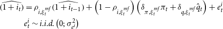 \begin{align} \widehat{\left ( 1+i_{t}\right ) } &=\rho _{i,\xi ^{mf}_t}\widehat{\left ( 1+i_{t-1}\right ) }+\left ( 1-\rho _{i,\xi ^{mf}_t}\right ) \left ( \delta _{\pi,\xi ^{mf}_t}\pi _{t}+\delta _{q,\xi ^{mf}_t}\hat{q}_{t}\right ) +e_{t}^{i} \\ &e_{t}^{i}\sim i.i.d.\left ( 0;\,\sigma _{e^i}^{2}\right ) \notag \end{align}
where $\widehat{\left ( 1+i_{t}\right ) }$
is the deviation of the monetary policy factor from its steady-state value,
$\widehat{\left ( 1+i_{t}\right ) }$
is the deviation of the monetary policy factor from its steady-state value, $\delta _{\pi }\gt 1$
and
$\delta _{\pi }\gt 1$
and $\delta _{q}\geq 0$
denote the policy reaction parameters to inflation and the bubble (
$\delta _{q}\geq 0$
denote the policy reaction parameters to inflation and the bubble ( $\delta _{q}\gt 0$
indicates a LAW policy), and
$\delta _{q}\gt 0$
indicates a LAW policy), and $\rho _{i}$
captures the persistence of the policy rate.Footnote
23
We set the policy reaction to inflation and the bubble and the policy persistence as functions of the two-state Markov process,
$\rho _{i}$
captures the persistence of the policy rate.Footnote
23
We set the policy reaction to inflation and the bubble and the policy persistence as functions of the two-state Markov process, $\xi ^{mf}_t\in \{\text{H-fin},\text{L-fin}\}$
, which jointly affects the steady-state bubble-to-output ratio. This process evolves according to a transition matrix,
$\xi ^{mf}_t\in \{\text{H-fin},\text{L-fin}\}$
, which jointly affects the steady-state bubble-to-output ratio. This process evolves according to a transition matrix, $H^{mf}$
, whose calibration is given by the VAR estimates, and which delivers monetary-financial regimes.
$H^{mf}$
, whose calibration is given by the VAR estimates, and which delivers monetary-financial regimes.
3.3. Solution method
We solve the model using the efficient perturbation methods applied to Markov-switching models elaborated by Maih (Reference Maih2015) and Foerster et al. (Reference Foerster, Rubio-Ramirez, Waggoner and Zha2016).Footnote 24 A detailed description of the solution method is reported in Appendix H. The model’s first-order approximated solution can be written in the following form:
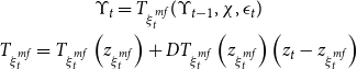 \begin{gather} \Upsilon _t=T_{\xi _t^{mf}}(\Upsilon _{t-1},\chi,\epsilon _t)\\ T_{\xi _t^{mf}}=T_{\xi _t^{mf}}\left (z_{\xi _t^{mf}}\right )+DT_{\xi _t^{mf}}\left (z_{\xi _t^{mf}}\right )\left (z_t-z_{\xi _t^{mf}}\right ) \notag \end{gather}
where $\Upsilon _t$
is the vector of model variables,
$\Upsilon _t$
is the vector of model variables, $T_{\xi _t^{mf}}$
the Taylor first-order expansion,
$T_{\xi _t^{mf}}$
the Taylor first-order expansion, $\chi$
defines the perturbation parameter,
$\chi$
defines the perturbation parameter, $\epsilon _t$
the vector of structural shocks, and
$\epsilon _t$
the vector of structural shocks, and $DT$
the matrix of first-order derivatives. The expansion point,
$DT$
the matrix of first-order derivatives. The expansion point, $z_{\xi _t^{mf}}=(\Upsilon,0,0)$
, is the vector of the steady states of the state variables,
$z_{\xi _t^{mf}}=(\Upsilon,0,0)$
, is the vector of the steady states of the state variables, $z_t=(\Upsilon _{t-1},\sigma,\epsilon _t)$
. As in Aruoba et al. (Reference Aruoba, Cuba-Borda and Shorfeide2018), where both a targeted-inflation steady state and a deflationary steady state are considered, we expand around two steady states per regime.
$z_t=(\Upsilon _{t-1},\sigma,\epsilon _t)$
. As in Aruoba et al. (Reference Aruoba, Cuba-Borda and Shorfeide2018), where both a targeted-inflation steady state and a deflationary steady state are considered, we expand around two steady states per regime.
3.4. Model-based impulse responses
We compute the impulse response functions to the monetary policy shock. We calibrate the model at the annual frequency by fixing $\beta =0.96$
,
$\beta =0.96$
, $\alpha =0.33$
,
$\alpha =0.33$
, $\gamma _b=1$
,
$\gamma _b=1$
, $g_s=1.02$
,
$g_s=1.02$
, $\gamma _s=0.2$
,
$\gamma _s=0.2$
, $\mu =1-1/42$
,
$\mu =1-1/42$
, $\delta _k=0.1$
,
$\delta _k=0.1$
, $\beta _{\text{beq}}=42$
,
$\beta _{\text{beq}}=42$
, $\phi =0.03$
,
$\phi =0.03$
, $A_2=0.3$
,
$A_2=0.3$
, $\sigma _i=0.01$
. The transition probabilities are fixed at the annual counterparts of the MS-VAR quarterly estimates: the probability of moving from the high to the low finance regime is thus 0.1834 and that from the low to the high 0.4205.
$\sigma _i=0.01$
. The transition probabilities are fixed at the annual counterparts of the MS-VAR quarterly estimates: the probability of moving from the high to the low finance regime is thus 0.1834 and that from the low to the high 0.4205.
The Markov-switching parameters, $\omega$
,
$\omega$
, $\rho _i$
,
$\rho _i$
, $\delta _\pi$
, and
$\delta _\pi$
, and $\delta _q$
, are estimated using a novel regime-dependent impulse response matching algorithm, mapping model-implied impulse responses to VAR results. More specifically, we match four regime-dependent VAR impulse responses: output, inflation, interest rate, and the bubble component of asset prices. Table 2 reports the results.
$\delta _q$
, are estimated using a novel regime-dependent impulse response matching algorithm, mapping model-implied impulse responses to VAR results. More specifically, we match four regime-dependent VAR impulse responses: output, inflation, interest rate, and the bubble component of asset prices. Table 2 reports the results.
Table 2. Model calibration based on impulse response-matching
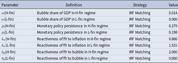
The estimated values are generated by matching the regime-dependent impulse responses of output, inflation, interest rate, and the asset price bubble component. Weights are based on their confidence intervals.
The estimation leads to a regime of high finance corresponding to a bubbly economy with a more persistent and less reactive monetary policy rule for inflation and displaying a LAW monetary policy rule ( $\delta _q\gt 0$
). Under this regime, the stationary level of the bubble is high enough to locate the economy in a crowding-in mode, with higher stationary levels of real rates, capital, and output. Instead, the L-fin regime corresponds to a no-bubbly economy, with policy rates targeting more actively inflation and lower interest rate persistence. This result provides further insight into Galì and Gambetti (Reference Galì and Gambetti2015)’s main conclusion.
$\delta _q\gt 0$
). Under this regime, the stationary level of the bubble is high enough to locate the economy in a crowding-in mode, with higher stationary levels of real rates, capital, and output. Instead, the L-fin regime corresponds to a no-bubbly economy, with policy rates targeting more actively inflation and lower interest rate persistence. This result provides further insight into Galì and Gambetti (Reference Galì and Gambetti2015)’s main conclusion.
Given the above calibration for the two states, Figure 5 shows the model-based impulse responses in the two regimes compared to the VAR counterparts. Following a positive shock to the nominal interest rate, the model predicts a recession/deflation and an increase in the real rate.Footnote 25 More importantly, in a bubble economy (H-fin regime) the contractionary monetary policy inflates bubbles’ valuation, in line with our empirical evidence in Section 2.
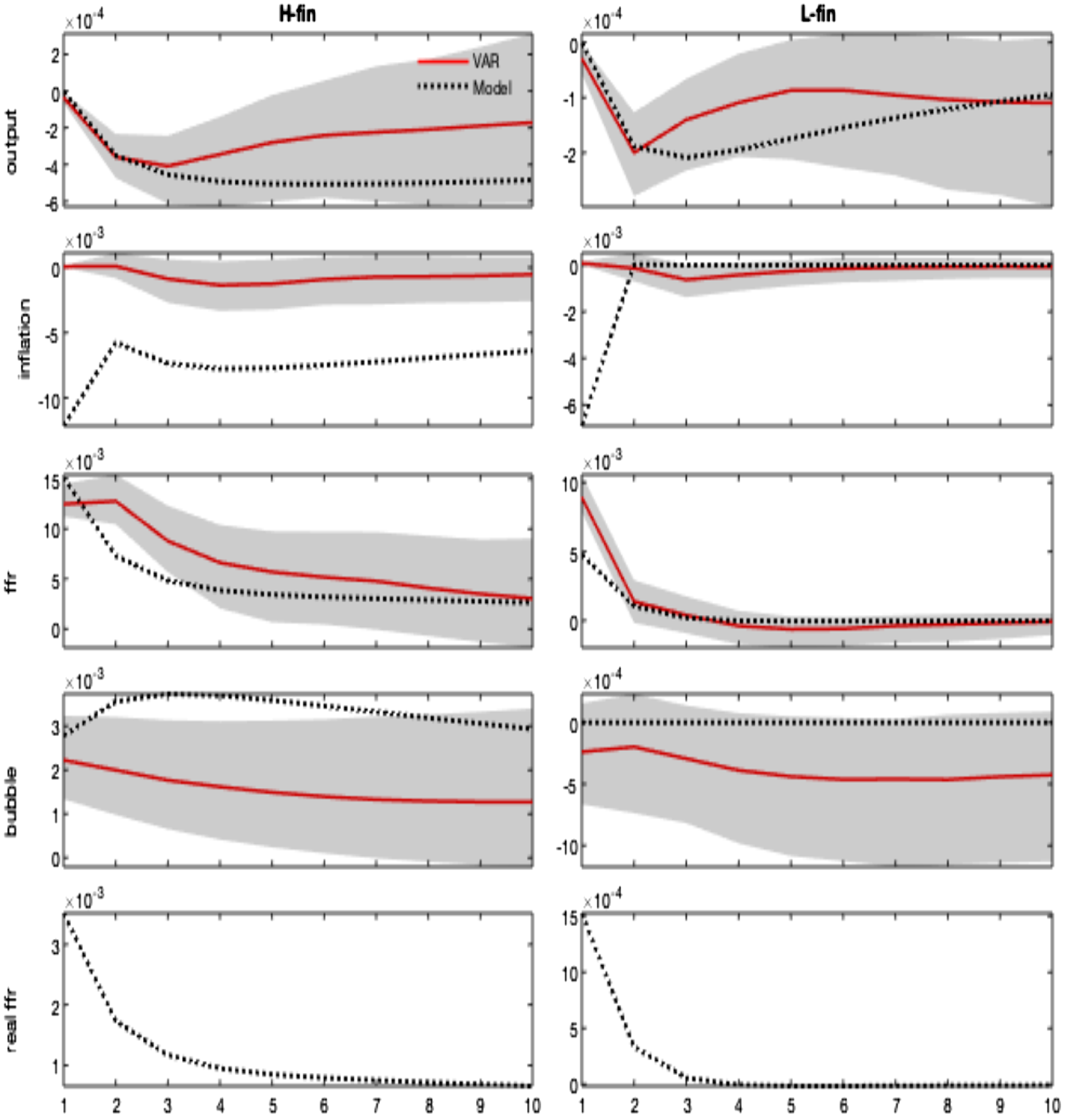
Figure 5. Monetary policy shock. Regime-dependent impulse responses. Notes: The figure shows the model-implied versus VAR-based impulse responses of selected variables (output, inflation, nominal interest rate, bubble, and the real interest rate) to a 1% monetary policy shock. Regimes affect the steady state parameter $\omega$
and the monetary policy rule, namely
$\omega$
and the monetary policy rule, namely $\rho _i$
,
$\rho _i$
, $\delta _{\pi }$
and
$\delta _{\pi }$
and $\delta _q$
. The impulse response matching is based on the following grid:
$\delta _q$
. The impulse response matching is based on the following grid: $\omega (\text{H-fin})\in [0,0.018]$
,
$\omega (\text{H-fin})\in [0,0.018]$
, $\omega (\text{L-fin})\in [0,0.01]$
,
$\omega (\text{L-fin})\in [0,0.01]$
, $\rho _i(\text{H-fin})\in [0.3,0.6]$
,
$\rho _i(\text{H-fin})\in [0.3,0.6]$
, $\rho _i(\text{L-fin})\in [0.1,0.3]$
,
$\rho _i(\text{L-fin})\in [0.1,0.3]$
, $\delta _q(\text{H-fin})\in [0,0.2]$
,
$\delta _q(\text{H-fin})\in [0,0.2]$
, $\delta _q(\text{L-fin})\in [0,2]$
,
$\delta _q(\text{L-fin})\in [0,2]$
, $\delta _\pi (\text{H-fin})\in [0.8,2]$
,
$\delta _\pi (\text{H-fin})\in [0.8,2]$
, $\delta _\pi (\text{L-fin})\in [1.25,2]$
. The corresponding loss function, computed on the distance between VAR and model-based impulse responses at the estimates, is equal to 0.1438. Shaded areas denote 68% credibility sets.
$\delta _\pi (\text{L-fin})\in [1.25,2]$
. The corresponding loss function, computed on the distance between VAR and model-based impulse responses at the estimates, is equal to 0.1438. Shaded areas denote 68% credibility sets.
The economic mechanism underlying these results is as follows: the monetary policy shock has a direct impact on the real interest rate, due to the nominal rigidity. In addition to the demand channel acting through the Euler equation and favoring future consumption, the increase in the real interest rate generates two additional effects: the demand for credit is reduced due to a price channel (the increased cost of borrowed funds); the value of the bubble rises, and an allocation channel redirects more resources toward the purchase of the bubble. These recessive channels more than compensate for the effect of the increase in the bubble size on credit demand due to the slackening of the collateral constraint, which allows borrowers to demand more funds (collateral channel). The outcome is a recession/deflation coupled with a rise in the bubble value. The policy reaction to the fall in inflation tends to mitigate the recessionary effects of the shock by reducing the amplitude of the downturn of output and inflation.
The recession/deflation and the increase in the real rate (and hence in the bubble component) are magnified when $\rho _{i}\gt 0$
and/or
$\rho _{i}\gt 0$
and/or $\delta _{q}\gt 0$
, namely under the high finance regime. The reason is that, following the exogenous interest rate shock, the policy reaction is dampened by the higher policy persistence and by the response to the bubble. Under LAW, the signal sent from the fall of inflation, which calls for a reduction of the real rate, is partially offset by the increase in the bubble component. The response of the central bank results in an effort that is too feeble in stabilizing the real interest rate. This result explains more persistence in the nominal interest rate response, higher real rates, and more severe recession/deflation compared to the L-finance regime. In a no-bubbly economy, interest rates respond to inflation only (and more than in H-fin), dampening the initial effects of the shock.
$\delta _{q}\gt 0$
, namely under the high finance regime. The reason is that, following the exogenous interest rate shock, the policy reaction is dampened by the higher policy persistence and by the response to the bubble. Under LAW, the signal sent from the fall of inflation, which calls for a reduction of the real rate, is partially offset by the increase in the bubble component. The response of the central bank results in an effort that is too feeble in stabilizing the real interest rate. This result explains more persistence in the nominal interest rate response, higher real rates, and more severe recession/deflation compared to the L-finance regime. In a no-bubbly economy, interest rates respond to inflation only (and more than in H-fin), dampening the initial effects of the shock.
3.5. Policy credibility and uncertainty scenarios
Our empirical and theoretical results are obtained under the hypothesis that stock market bubbles exist and can be measured, at least indirectly. A recent macro-finance literature [e.g., Jarrow (Reference Jarrow2016), Jarrow et al. (Reference Jarrow, Kchia and Protter2011a, Reference Jarrow, Kchia and Protterb), Jarrow and Kwok (Reference Jarrow and Kwok2021), Fusari et al. (Reference Fusari, Jarrow and Lamichhanne2022)] provides several convincing contributions on the existence of bubbles. However, the proliferating bubble detection methods testify that measurement issues are far from being solved. Uncertainty about the empirical reliability of specific bubble component’s evaluation methods is a pervading limitation our analysis shares with previous contributions. To widen its validity domain, we test the robustness of our results against alternative assumptions regarding the monetary-financial regimes and the agents’ capacity to observe them.
In the first set of counterfactual scenarios, we assess the role of agents’ beliefs on macroeconomic dynamics under the two regimes, by comparing the benchmark impulse responses to scenarios built by varying the probability distribution of regimes. Being part of their information set, they may depend on policy credibility. A second set of counterfactuals is used to consider the role of uncertainty around the realization of regimes, hence the existence and valuation of a bubble. In this case, we depart from the standard rational expectations assumption that agents can observe the true transition matrix for monetary-financial regime shifts and assume that they are uncertain about how long any observed regime shift will last and hence must learn about its duration. We do so by comparing the benchmark impulse responses to those built under learning, passing from the perception of a short-lived to a long-lived high finance regime. To complement the analysis, we evaluate the same counterfactuals for the case of a monetary authority setting the interest rate disregarding bubbles, even when they exist.
More specifically, in the first set of scenarios in Figure 6, the transition matrix is modified such that agents attach different probabilities to the occurrence of a regime change. We label as “H-fin credible” the scenario where we set to zero the probability of going from H-fin to L-fin and increase by 50% that of transitioning from L-fin to H-fin (from 0.1834 to 0.2751). We label as “L-fin credible” the scenario where we set to 0.01 the probability to go from L-fin to H-fin and increase by 50% that of transitioning from H-fin to L-fin (from 0.4205 to 0.6307).
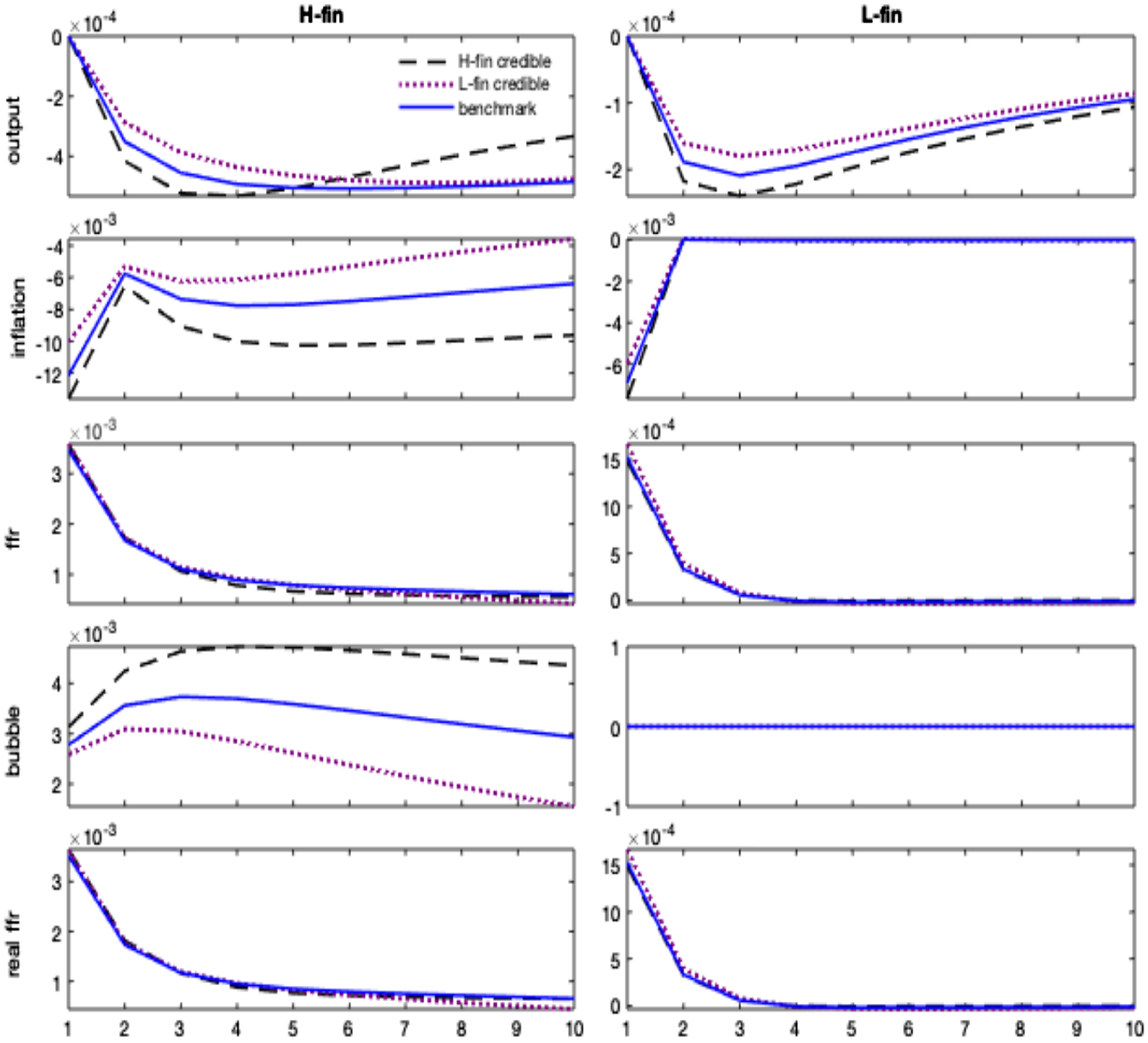
Figure 6. Impulse responses to monetary policy shock. Counterfactual scenarios on policy credibility. Notes: The figure compares the impulse responses extracted from the estimated model to those from counterfactual scenarios defined as follows: an H-fin credible scenario increases the probability of switching from L-fin to H-fin and decreases the probability from H-fin to L-fin; an L-fin credible scenario increases the probability to switch from H-fin to L-fin and decrease the probability from L-fin to H-fin.
The credibility of announcing a different policy can significantly affect the efficacy of the current policy stance. When agents expect the high finance policy ( $\rho _i\gt 0$
,
$\rho _i\gt 0$
, $\delta _q\gt 0$
) to last longer (H-fin credible), the effect of a monetary policy shock is exacerbated both in terms of deeper recession/deflation and bubble’s inflation. In the long run, the increase in asset valuation boosts the borrowing capacity and favors a faster exit from the crisis. Suppose, instead, that in response to an announced shift toward a stabilizing regime (low finance), agents assign a higher probability to switch to the low finance regime (L-fin credible). In that case, they also assign a higher probability to the belief that the policy rule will be more stabilizing in the future. Hence, they may start disinvesting in the bubbly asset in anticipation, effectively raising the probability of switching to the no-bubble scenario. This result makes the deflationary and recessive effects of the monetary policy shock smoother. In a nutshell, in a bubbly world, the impact of monetary tightening depends on how agents form their beliefs on the credibility of the monetary policy and the state of the bubble.
$\delta _q\gt 0$
) to last longer (H-fin credible), the effect of a monetary policy shock is exacerbated both in terms of deeper recession/deflation and bubble’s inflation. In the long run, the increase in asset valuation boosts the borrowing capacity and favors a faster exit from the crisis. Suppose, instead, that in response to an announced shift toward a stabilizing regime (low finance), agents assign a higher probability to switch to the low finance regime (L-fin credible). In that case, they also assign a higher probability to the belief that the policy rule will be more stabilizing in the future. Hence, they may start disinvesting in the bubbly asset in anticipation, effectively raising the probability of switching to the no-bubble scenario. This result makes the deflationary and recessive effects of the monetary policy shock smoother. In a nutshell, in a bubbly world, the impact of monetary tightening depends on how agents form their beliefs on the credibility of the monetary policy and the state of the bubble.
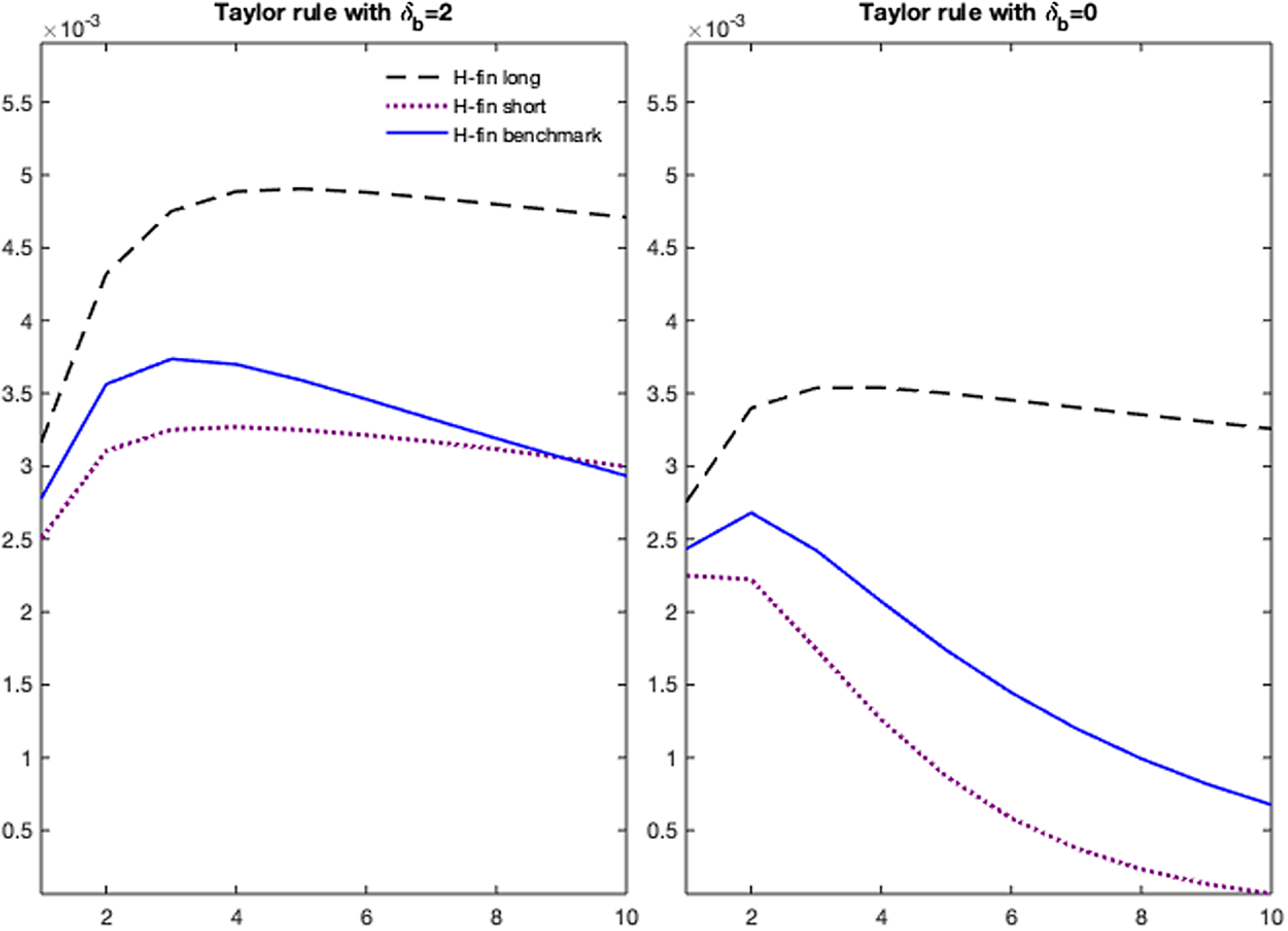
Figure 7. Impulse responses of the bubble to a monetary policy shock in high finance regime. Counterfactual scenarios on regime uncertainty. Notes: The figure compares the benchmark impulse response of the bubble to the monetary policy shock in the high finance regime to those from two counterfactual scenarios defined as follows: an H-fin long scenario where the probability of going from H-fin to H-fin long-lasting is 0.99, and the probability of going from H-fin temporary to the L-fin regime is 0.01; an H-fin short scenario where the probability of going from H-fin temporary to H-fin long-lasting is 0.01, and the probability of going from H-fin temporary to the L-fin regime is 0.4205. The left panel performs the counterfactual scenarios with a monetary policy rule targeting the bubble, as from the impulse response matching, $\delta _b=2$
. The right panel assumes the monetary authority does not respond to the bubble,
$\delta _b=2$
. The right panel assumes the monetary authority does not respond to the bubble, $\delta _b=0$
.
$\delta _b=0$
.
In the second set of counterfactual scenarios, we model the idea that agents can still observe the regime in place at each point in time. However, they face uncertainty about the nature of deviations from the low finance regime. Namely, they are unsure if the central bank is engaging in a short or long-lasting high finance regime. This simulation introduces a learning mechanism on the persistence of regime changes [Bianchi et al. (Reference Bianchi, Lettau and Ludvigson2022)], by expanding the number of regimes to account for short- or long-lasting perceived high finance regimes.Footnote
26
We use three states: a low finance regime, a short-lasting, and a long-lasting high finance regime. Uncertainty arises because the two high finance regimes share the same parameter values governed by $\xi ^{mf}$
, which agents recognize as belonging to a high finance regime. However, they cannot precisely infer whether it is a short- or long-lasting high finance regime. This is something they learn after switching to the new regime. After the switch to high finance, agents initially perceive it as a temporary deviation while adjusting only afterward to persistent changes.
$\xi ^{mf}$
, which agents recognize as belonging to a high finance regime. However, they cannot precisely infer whether it is a short- or long-lasting high finance regime. This is something they learn after switching to the new regime. After the switch to high finance, agents initially perceive it as a temporary deviation while adjusting only afterward to persistent changes.
In Figure 7, we compare the bubble impulse response to a monetary tightening in the high finance regime (blue line), under the estimated VAR-based calibration, to those when it is perceived as temporary (purple dotted) and long lasting (black dashed). In the first case, we assume a transition matrix where the probability of going from the temporary to the long-lasting high finance regime is 0.01, and the probability of going from short-lasting high finance to the low finance regime is 0.4205. We denote this as the “H-fin short scenario”. In the second case, we assume the probability of going from H-fin temporary to H-fin long-lasting is 0.99, and the probability of going from H-fin temporary to the L-fin regime is 0.01. We denote this scenario as an “H-fin long scenario”.
Learning about the persistence of the high finance regime implies that bubbles in the model respond to shifts to the high finance regime by initially underreacting to the monetary policy shock (short-lasting scenario) compared to the benchmark high finance response. Then, when they realize the shift is more persistent, they tend to overreact. We run the same counterfactual scenarios on a model where the central bank does not target the financial cycle and disregards bubble dynamics ( $\delta _b=0$
). Both in the benchmark VAR-based version of the transition matrix and in the counterfactual scenarios on the duration of the high finance regime, the bubble response to a monetary policy shock is lower and less persistent, thus reinforcing our argument against the LAW policy.
$\delta _b=0$
). Both in the benchmark VAR-based version of the transition matrix and in the counterfactual scenarios on the duration of the high finance regime, the bubble response to a monetary policy shock is lower and less persistent, thus reinforcing our argument against the LAW policy.
4. Conclusions
This paper contributes to the empirical evidence showing that an unexpected monetary tightening determines an increase in the stock price’s bubble component. By estimating a Markov-switching structural vector autoregressive model over U.S. data, we find that regimes of high stock prices and equity returns are those in which a monetary policy tightening leads to higher fluctuations in real macroeconomic variables and inflation, together with an increase in the bubbly component of the stock price. That more than offsets the decline in the fundamental component in the medium to long term. This result is described over identified regime-shift events in the history of the U.S. monetary and financial facts.
We then use a model for rational bubbles to match and rationalize the empirical findings. The model predicts that a monetary tightening proves ineffective in reducing stock prices in a bubbly economy, increasing real rates. Under this state, monetary policy is less reactive to inflation, favoring more persistent recession/deflation. The outcome is a more severe recession/deflation coupled with a rise in the bubble value.
Counterfactual scenarios on policy credibility show that if agents believe that the transition to a bubbly regime is more likely, a monetary policy shock is exacerbated in terms of deeper recession/deflation and bubble inflation. Instead, if agents face uncertainty about the duration of regimes, a gradual adjustment in the bubble valuation is observed after the regime shift dates, until explaining an overreaction of the bubble to the monetary impulse. Despite the limitations of the analysis coming from the unresolved empirical issue on bubble detection, these additional checks help interpreting our findings in the context of a realistic policy making.
Appendices
A. Data
We use quarterly US data spanning the period 1960–2019. The six variables included in the MS-SVAR are: log-real GDP $y_{t}$
, log-real dividends
$y_{t}$
, log-real dividends $d_{t}$
, the GDP deflator inflation
$d_{t}$
, the GDP deflator inflation $\pi _{t}^{y}$
, the inflation rate for non-energy commodities
$\pi _{t}^{y}$
, the inflation rate for non-energy commodities $\pi _{t}^{c}$
, the federal funds rate
$\pi _{t}^{c}$
, the federal funds rate $r_{t}$
, and the log-real S&P500 index
$r_{t}$
, and the log-real S&P500 index $q_{t}$
. For the policy rate, we control for non-conventional measures by taking the Wu and Xia (Reference Wu and Xia2016) shadow interest rate over the 2009–2016 time interval. Table A1 below summarizes the variable’s data sources and their transformations in the estimates.
$q_{t}$
. For the policy rate, we control for non-conventional measures by taking the Wu and Xia (Reference Wu and Xia2016) shadow interest rate over the 2009–2016 time interval. Table A1 below summarizes the variable’s data sources and their transformations in the estimates.
Table A1. Data sources and their transformations
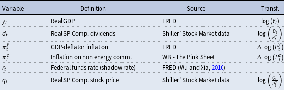
B. MS-SBVAR. Model selection
We select the best-fit model by comparing the fit of several Markov-switching SVARs through marginal data densities (MDD), namely the probability of the data after integrating out the parameters in the model:
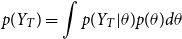 \begin{equation*} p(Y_T)=\int p(Y_T|\theta )p(\theta )d\theta \end{equation*}
where $\theta$
is the vector of the SVAR parameters,
$\theta$
is the vector of the SVAR parameters, $p(Y_T|\theta )$
is the likelihood function, and
$p(Y_T|\theta )$
is the likelihood function, and $p(\theta )$
is the priors. The modified harmonic mean (MHM) method of Gelfand and Dey (Reference Gelfand and Dey1994) is based on the following theoreom:
$p(\theta )$
is the priors. The modified harmonic mean (MHM) method of Gelfand and Dey (Reference Gelfand and Dey1994) is based on the following theoreom:
 \begin{equation*} p(Y_T)^{-1}=\int \frac {h(\theta )}{p(Y_T|\theta )p(\theta )}p(\theta |Y_T)d\theta \end{equation*}
where $p(\theta |Y_T)$
is the posterior distribution, and
$p(\theta |Y_T)$
is the posterior distribution, and $h(\theta )$
is a weighting function chosen to deliver the following Monte Carlo integration:
$h(\theta )$
is a weighting function chosen to deliver the following Monte Carlo integration:
 \begin{equation*} p(Y_T)^{-1}=\frac {1}{N} \sum _{i=1}^{N}\frac {h(\theta )}{p(Y_T|\theta )p(\theta )} \end{equation*}
Alternative methods to compute the MDD differ in the weighting function used for this numerical approximation since, in Markov-switching models, the posterior is highly multimodal and contains zeros in the interior points of the parameter space. In Table B1, we, therefore, evaluate MDDs over three metrics: the new modified harmonic mean method (MHM) suggested by Sims and Zha (Reference Sims and Zha2006), Meng and Wong (Reference Meng and Wong1996)’s bridge sampling method, and the Muller’s method [Liu et al. (Reference Liu, Waggoner and Zha2011)]. They are compared to the fit of a constant-coefficient model using the Chib (Reference Chib1995)’s method.Footnote 27
Table B1. Marginal Data Densities for model selection
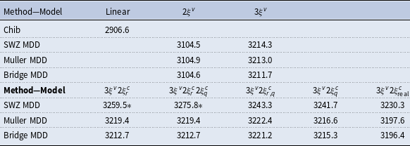
The table reports the log MDDs associated with different models under the new modified harmonic mean, the bridge, and Müller methods. The Markov-switching models under assessment are defined as follows: a two-state Markov chain on all shock variances ( $2\xi ^{v}$
); a three-state chain on all shock variances
$2\xi ^{v}$
); a three-state chain on all shock variances $\left(3\xi ^{v}\right)$
; two independent Markov chains, one three-state chain on all shock variances and a two-state chain on the interest rate equation (
$\left(3\xi ^{v}\right)$
; two independent Markov chains, one three-state chain on all shock variances and a two-state chain on the interest rate equation ( $3\xi ^{v},2\xi ^{c}_r$
); three independent Markov chains, one three-state chain on all shock variances, a two-state chain on the interest rate equation and one chain governing asset price equation (
$3\xi ^{v},2\xi ^{c}_r$
); three independent Markov chains, one three-state chain on all shock variances, a two-state chain on the interest rate equation and one chain governing asset price equation ( $3\xi ^{v}2\xi ^c_{r}2\xi ^c_{q}$
); two independent Markov chains, one three-state chain on all shock variances and a two-state chain jointly on the interest rate and the asset price equations (
$3\xi ^{v}2\xi ^c_{r}2\xi ^c_{q}$
); two independent Markov chains, one three-state chain on all shock variances and a two-state chain jointly on the interest rate and the asset price equations ( $3\xi ^{v},2\xi ^c_{r,q}$
); two independent Markov chains, one three-state chain on all shock variances and a two-state chain on the asset price equation (
$3\xi ^{v},2\xi ^c_{r,q}$
); two independent Markov chains, one three-state chain on all shock variances and a two-state chain on the asset price equation ( $3\xi ^{v},2\xi ^c_{r}$
); two independent Markov chains, one three-state chain on all shock variances and a two-state chain on the equations defining the real-sector variables
$3\xi ^{v},2\xi ^c_{r}$
); two independent Markov chains, one three-state chain on all shock variances and a two-state chain on the equations defining the real-sector variables $\left(3\xi ^{v},2\xi ^c_{\text{real}}\right)$
.
$\left(3\xi ^{v},2\xi ^c_{\text{real}}\right)$
.
A set of results can be extracted. First, all models with time-varying properties outperform the linear model. Second, a model with regime-switching variances with up to three states ( $3\xi ^v$
) improves substantially over the linear case but is dominated by models with regime switches in both the systematic and stochastic components. Third, introducing MS dynamics in the systematic model component featuring the real sector only worsens model fit when compared to the model with variance regimes only while introducing nonlinearities in the monetary policy or the asset price equations improves model performance
$3\xi ^v$
) improves substantially over the linear case but is dominated by models with regime switches in both the systematic and stochastic components. Third, introducing MS dynamics in the systematic model component featuring the real sector only worsens model fit when compared to the model with variance regimes only while introducing nonlinearities in the monetary policy or the asset price equations improves model performance $\left(3\xi ^v2\xi ^c_{r}, 3\xi ^v2\xi ^c_{q}\right)$
. Finally, it is the interaction of monetary and financial structural dynamics
$\left(3\xi ^v2\xi ^c_{r}, 3\xi ^v2\xi ^c_{q}\right)$
. Finally, it is the interaction of monetary and financial structural dynamics $\left(3\xi ^v2\xi ^c_{r,q}\right)$
that best describes our data, outperforming the independent alternative
$\left(3\xi ^v2\xi ^c_{r,q}\right)$
that best describes our data, outperforming the independent alternative $\left(3\xi ^v2\xi ^c_{r}2\xi ^c_{q}\right)$
.
$\left(3\xi ^v2\xi ^c_{r}2\xi ^c_{q}\right)$
.
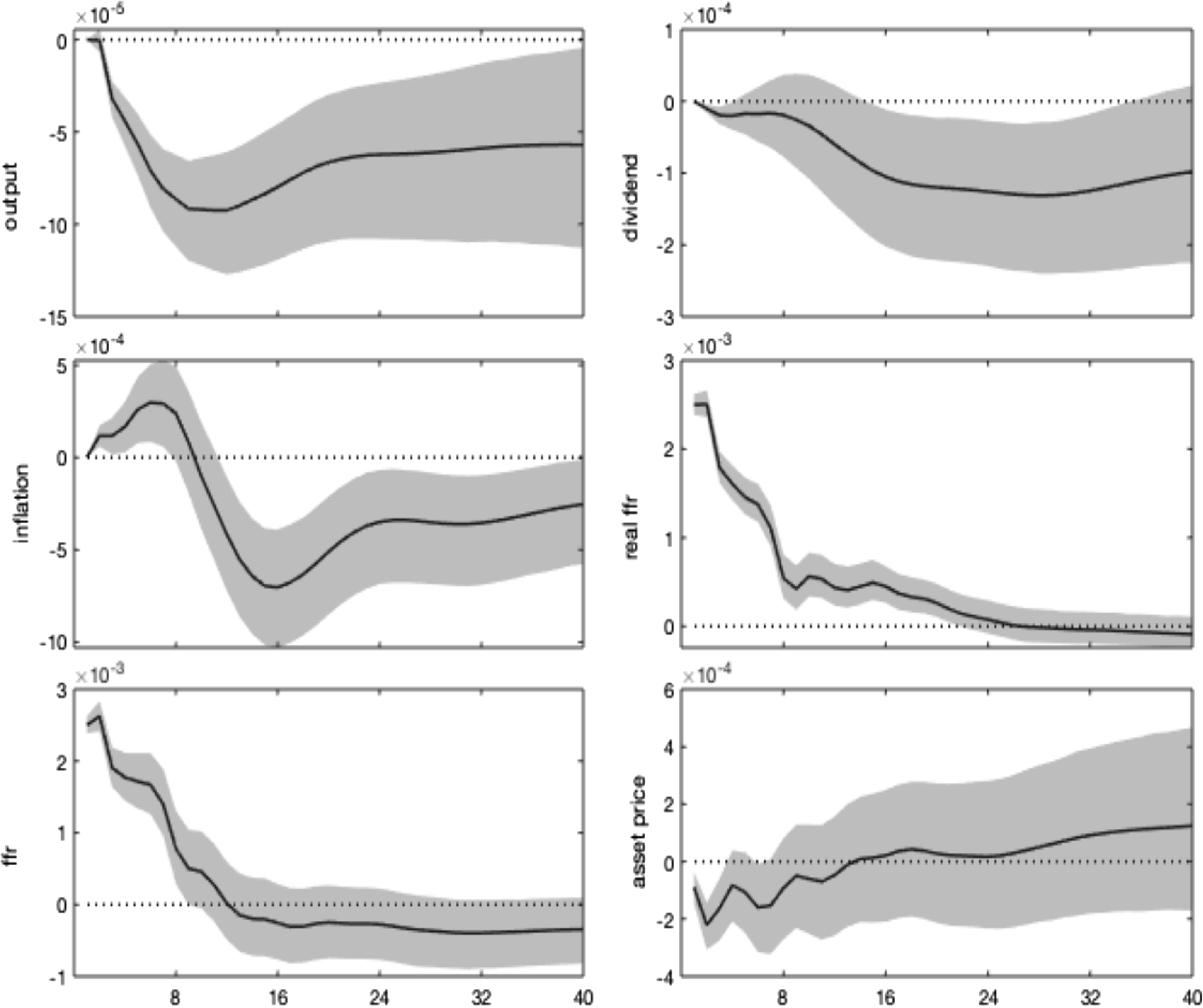
Figure C1. Monetary policy shock. Impulse responses. Notes: The figure shows the impulse responses to a 1% monetary policy shock. Shaded areas denote 68% credibility sets.
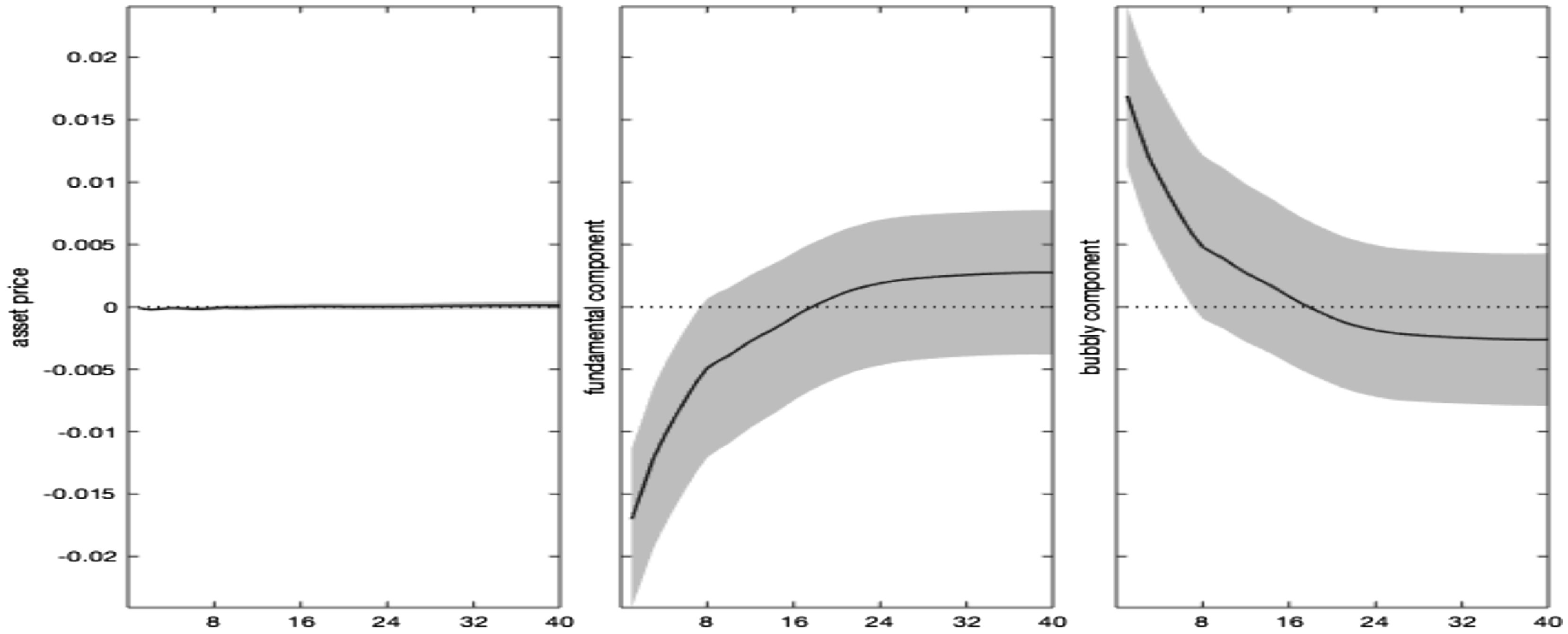
Figure C2. Monetary policy shock. Impulse responses: stock price decomposition. Notes: The figure shows the impulse responses of asset prices, and their decomposition in a fundamental and bubbly component, to a 1% monetary policy shock. Shaded areas denote 68% credibility sets.
C. MS-SBVAR. Linear model
We estimate a linear BVAR using the same data and identification strategy as in the Markov-switching model. In Figures C1 and C2 we simulate a 1% monetary policy shock and show that asset price fundamentals (dividends, real rates) react more weakly in a linear world, displaying moderate and less persistent responses. Moreover, the overall S&P500 response is negligible, leading to a residual bubble response completely offsetting the fundamental one. These results highlight that introducing regime changes amplifies the contribution of the fundamental asset price component to the build-up of the bubble.
D. MS-SBVAR. Time-varying equity premium
This section examines how our estimated deviation between observed stock prices and the measured fundamental component should be interpreted compared to the one resulting from considering a time-varying equity premium.
By computing the log-linearized excess stock returns as
 \begin{equation*}z_{t+1}=\Delta q_{t+1} + (1-\Delta )d_{t+1}-q_t-r_t\end{equation*}
Galì and Gambetti (Reference Galì and Gambetti2015) show that the dynamic response of the stock prices to an exogenous monetary policy shock as comprising the response of the equity premium:
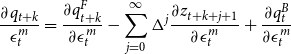 \begin{equation*}\frac {\partial q_{t+k}}{\epsilon ^m_t}=\frac {\partial q^F_{t+k}}{\partial \epsilon ^m_t}-\sum ^{\infty }_{j=0}\Delta ^j \frac {\partial z_{t+k+j+1}}{\partial \epsilon ^m_t} + \frac {\partial q^B_t}{\partial \epsilon ^m_t}\end{equation*}
where $\partial q^F_{t+k}/\partial \epsilon ^m_t= \sum _{j=0}^{\infty }\Delta ^j(1-\Delta )\partial d_{t+k+j+1}/\partial \epsilon ^m_t$
. The bubble response and the excess stock returns explain the gap between the observed asset price and its fundamental component. If excess returns respond positively to the monetary policy shock, the bubble response is higher than the one computed under the assumption of risk neutrality. Hence, the presence of a risk premium downplays the bubble evidence only if it declines substantially and persistently in response to a tightening of monetary conditions.
$\partial q^F_{t+k}/\partial \epsilon ^m_t= \sum _{j=0}^{\infty }\Delta ^j(1-\Delta )\partial d_{t+k+j+1}/\partial \epsilon ^m_t$
. The bubble response and the excess stock returns explain the gap between the observed asset price and its fundamental component. If excess returns respond positively to the monetary policy shock, the bubble response is higher than the one computed under the assumption of risk neutrality. Hence, the presence of a risk premium downplays the bubble evidence only if it declines substantially and persistently in response to a tightening of monetary conditions.
In line with the existing evidence [Bernanke and Kuttner (Reference Bernanke and Kuttner2005) and Caldara and Herbst (Reference Caldara and Herbst2019)], Figure D1 documents a positive response of the excess S&P500 stock return to the monetary policy shock. This result reflects the premium agents require for the higher risk they carry by investing in risky assets due to bonds becoming more attractive relative to stocks. Under the high finance regime, the positive response of the bubble more than offsets the positive risk premium response, which in turn enters negatively into the asset price response derivation. Hence, our evidence is emphasized in the presence of a risk premium component.
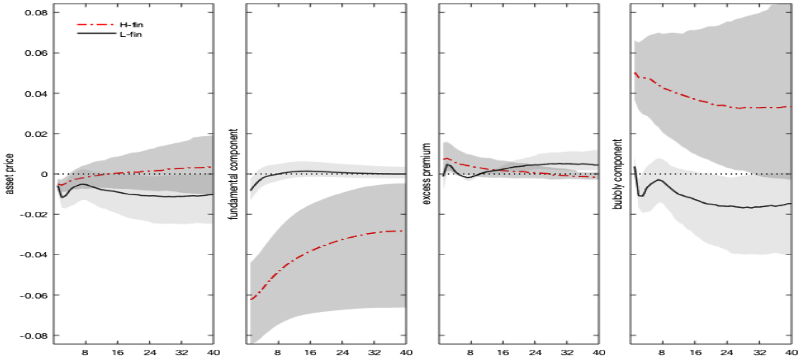
Figure D1. Monetary policy shock. Impulse responses: stock price decomposition. Notes: The figure shows the impulse responses of asset prices, and their decomposition in a fundamental and bubbly component, to a 1% monetary policy shock. Differences across regimes only reflect nonlinearities in the monetary policy and asset price equations, driven by $\xi ^{mf}$
. Shaded areas denote 68% credibility sets.
$\xi ^{mf}$
. Shaded areas denote 68% credibility sets.
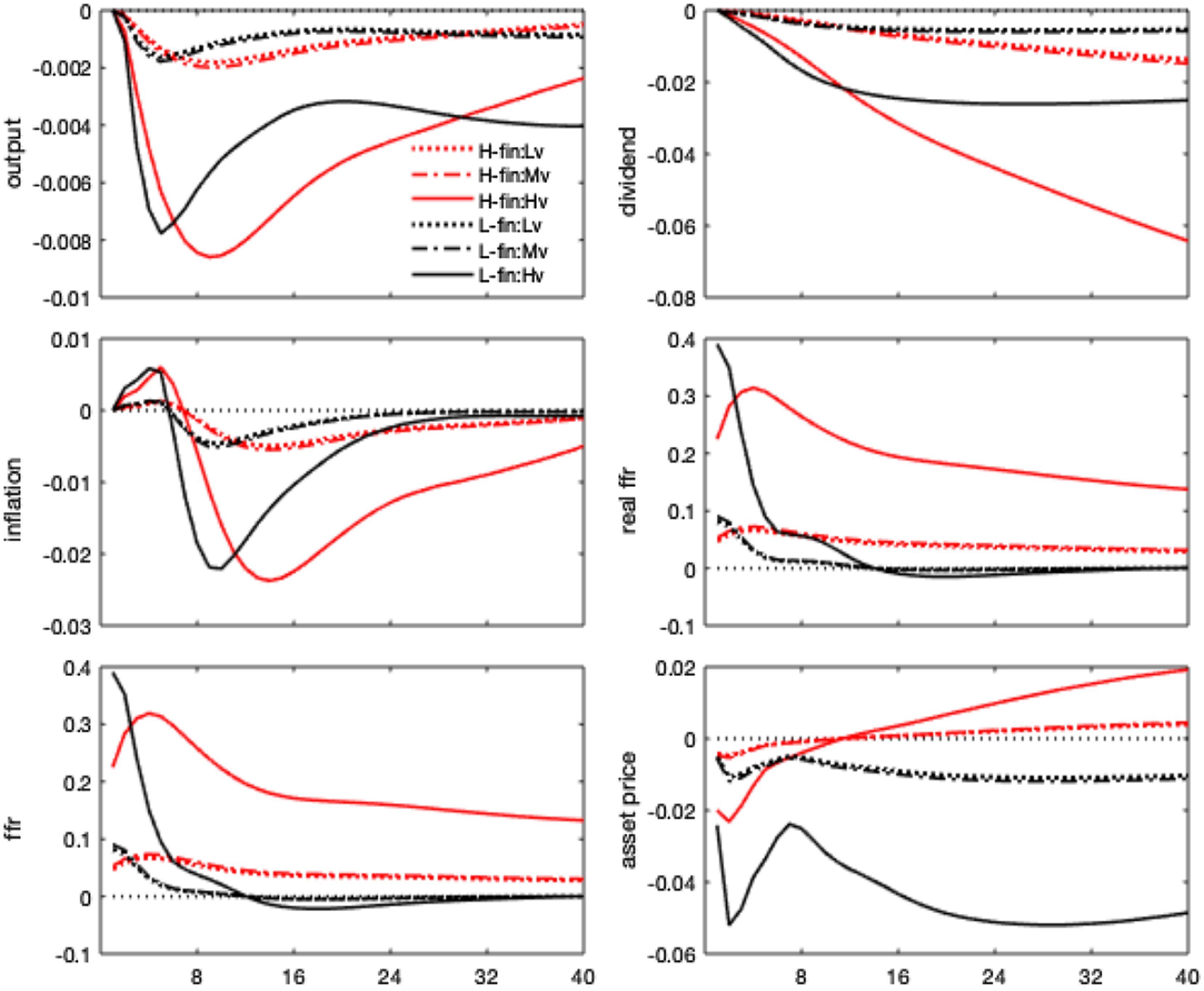
Figure E1. Monetary policy shock. Impulse responses. Notes: The figure shows the impulse responses to a monetary policy shock in the six combinations of regimes, hence driven by the composite Markov process $\xi =\{\xi ^{mf},\xi ^v\}\in \{\text{H-finance: L-variance, H-finance: M-variance, H-finance: H-variance}$
,
$\xi =\{\xi ^{mf},\xi ^v\}\in \{\text{H-finance: L-variance, H-finance: M-variance, H-finance: H-variance}$
, $\text{L-finance: L-variance,}$ $\text{L-finance: L-variance, L-finance: L-variance}\}$
.
$\text{L-finance: L-variance, L-finance: L-variance}\}$
.
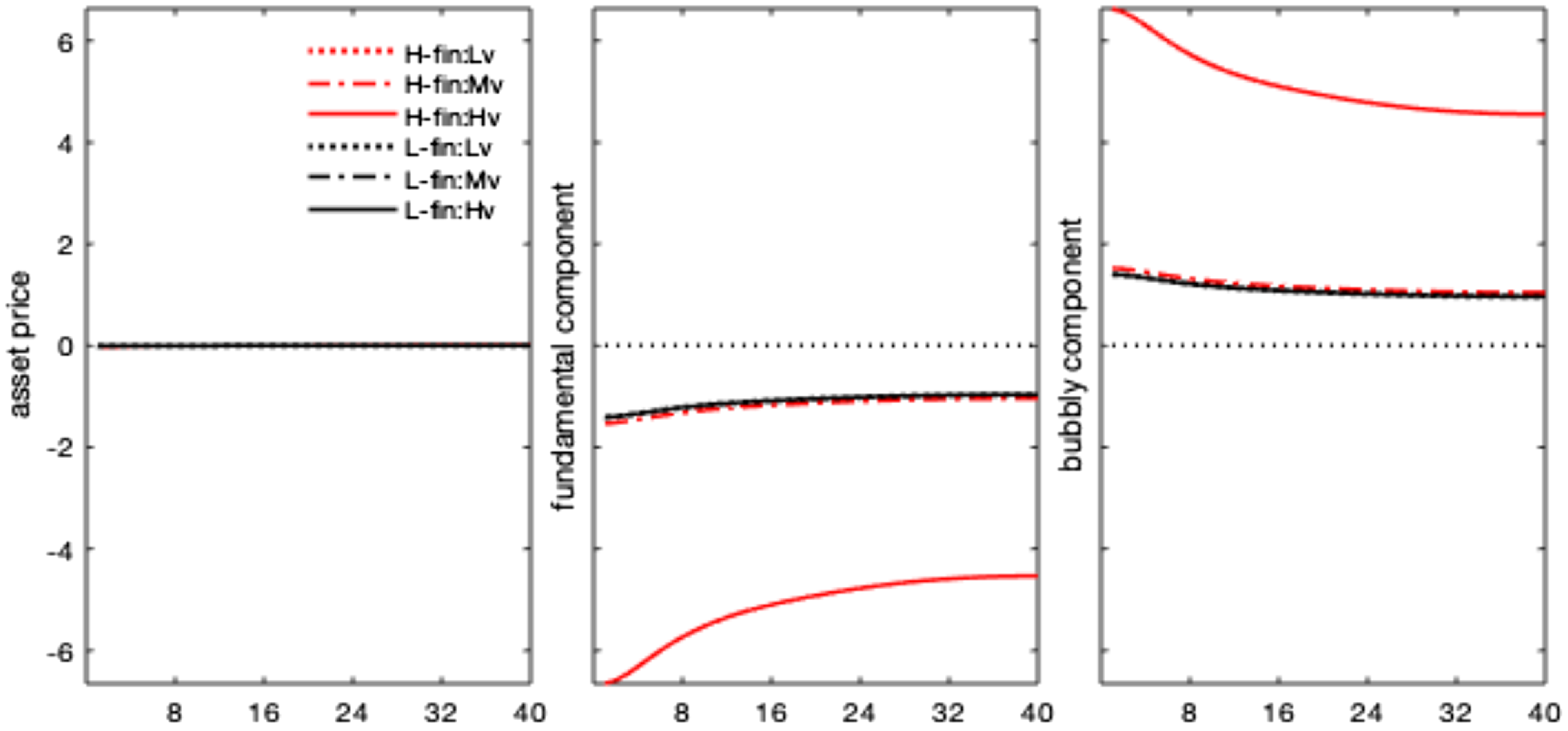
Figure E2. Monetary policy shock. Impulse responses: stock price decomposition. Notes: The figure shows the impulse responses of asset prices and their decomposition in a fundamental and bubbly component, to a monetary policy shock, in the six combinations of regimes, hence driven by the composite Markov process $\xi =\{\xi ^{mf},\xi ^v\}\in \{\text{H-finance: L-variance, H-finance: M-variance, H-finance: H-variance, L-finance: L-variance, L-finance: }$ $\text{L-variance, L-finance: L-variance}\}$
.
$\text{L-variance, L-finance: L-variance}\}$
.
E. MS-SBVAR. Impulse responses with variance regimes
In the VAR, regimes characterize the shocks’ size and their transmission mechanism, thus affecting both quantitatively and qualitatively model dynamics. Section 2.4 shows impulse responses to a 1% monetary policy shock in all regimes. This normalization rules out the impact of variance regimes and allows us to focus on systematic nonlinearities, namely the monetary-financial regimes. However, the combination of variance and coefficient regimes identifies six regions over the history of the data sample. Figures E1 and E2 display impulse responses accounting for each state.
Table F1. Forecast error variance decomposition—monetary policy shock. Low-variance state
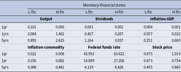
The table presents the fraction of variances (computed from the posterior median) of model variables explained by the monetary policy shock at various horizons under each regime. The results are for the low-variance state.
The state of high shocks’ variance vastly amplifies the size of impulse responses, both under the high finance and low finance regimes. However, the high finance-high variance state—prevailing in the 1970–1975 and 2008–2009 periods—adds persistence dynamics to the amplification, resulting in significant reversals in the fundamental/bubbly composition of the asset price response.
F. MS-SBVAR. Forecast error variance decomposition
Table F1 reports the forecast error variance decomposition for each state in the model systematic component, indicating the fraction of variance of model variables explained by the monetary policy shocks on impact at the 1-year and 5-year time horizons. The displayed results are for the low variance state only. The FEVDs show that the relevance of the policy shock is higher under the high finance state in the long term, being around 3% after 5 years when a monetary shock is more persistent, generates amplified effects, and stock prices contain an higher bubble share.
G. A model for bubbles
G.1. Savers/lenders
The following specifies the preferences of the representative saver utility function:Footnote 28
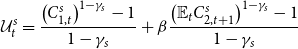 \begin{equation} \mathcal{U}_{t}^{s}=\frac{\left ( C_{1,t}^{s}\right ) ^{1-\gamma _{s}}-1}{1-\gamma _{s}}+\beta \frac{\left ( \mathbb{E}_{t}C_{2,t+1}^{s}\right ) ^{1-\gamma _{s}}-1}{1-\gamma _{s}} \end{equation}
where $\gamma _{s}\in \lbrack 0;1)$
is the inverse of the intertemporal elasticity of substitution,
$\gamma _{s}\in \lbrack 0;1)$
is the inverse of the intertemporal elasticity of substitution, $\beta \in \left ( 0;\,1\right )$
is the subjective discount factor, and
$\beta \in \left ( 0;\,1\right )$
is the subjective discount factor, and $\mathbb{E}_{t}$
represents the (conditional) expectation operator.
$\mathbb{E}_{t}$
represents the (conditional) expectation operator. $C_{1,2}^{s}$
is an index of the saver’s aggregate consumption of the final goods in the two periods:
$C_{1,2}^{s}$
is an index of the saver’s aggregate consumption of the final goods in the two periods:
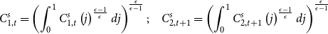 \begin{equation} C_{1,t}^{s}=\left ( \int _{0}^{1}C_{1,t}^{s}\left ( j\right ) ^{\frac{\epsilon -1}{\epsilon }}dj\right ) ^{\frac{\epsilon }{\epsilon -1}};\quad C_{2,t+1}^{s}=\left ( \int _{0}^{1}C_{2,t+1}^{s}\left ( j\right ) ^{\frac{\epsilon -1}{\epsilon }}dj\right ) ^{\frac{\epsilon }{\epsilon -1}} \end{equation}
where $\epsilon$
is the elasticity of substitution between the
$\epsilon$
is the elasticity of substitution between the $j$
-types of final goods.
$j$
-types of final goods.
The budget constraints are
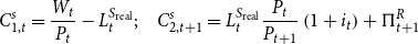 \begin{equation} C_{1,t}^{s}=\frac{W_{t}}{P_{t}}-L_{t}^{S_{\text{real}}};\quad C_{2,t+1}^{s}=L_{t}^{S_{\text{real}}}\frac{P_{t}}{P_{t+1}}\left ( 1+i_{t}\right ) +\Pi _{t+1}^{R} \end{equation}
where $L_{t}^{S_{\text{real}}}$
is the amount of savings,
$L_{t}^{S_{\text{real}}}$
is the amount of savings, $\frac{W_{t}}{P_{t}}$
is the real wage, and
$\frac{W_{t}}{P_{t}}$
is the real wage, and $\Pi _{t+1}^{R}$
are real profits.
$\Pi _{t+1}^{R}$
are real profits.
The optimization problem of savers is then:
 \begin{equation*} \max _{C_{1,t}^{s},C_{2,t+1}^{s},L_{t}^{S_{\text{real}}}}\mathcal {U}_{t}^{s}\,\text{s.t. (G9)} \end{equation*}
from the first-order conditions of this problem, the supply of funds (expressed in real terms) can be obtained:
 \begin{equation} L_{t}^{S_{\text{real}}}=\frac{\beta ^{\frac{1}{\gamma _{s}}}}{\beta ^{\frac{1}{\gamma _{s}}}+\left ( \mathbb{E}_{t}R_{t+1}\right ) ^{1-\frac{1}{\gamma _{s}}}}\left ( \frac{W_{t}}{P_{t}}-\frac{\mathbb{E}_{t}\left ( \Pi _{t+1}^{R}\right ) }{\beta ^{\frac{1}{\gamma _{s}}}\left ( \mathbb{E}_{t}R_{t+1}\right ) ^{\frac{1}{\gamma _{s}}}}\right ) \end{equation}
where $R_t=\frac{P_{t}}{P_{t+1}}\left ( 1+i_{t}\right )$
is the real interest rate.
$R_t=\frac{P_{t}}{P_{t+1}}\left ( 1+i_{t}\right )$
is the real interest rate.
G.2. Borrowers/investors
We assume that, differently from savers, borrowers leave resources $S_{t+1}\geq 0$
to the next generation:Footnote
29
$S_{t+1}\geq 0$
to the next generation:Footnote
29
 \begin{equation} \mathcal{U}_{t}^{b}=\frac{\left ( C_{1,t}^{b}\right ) ^{1-\gamma _{b}}-1}{1-\gamma _{b}}+\beta \frac{\left ( \mathbb{E}_{t}C_{2,t+1}^{b}\right ) ^{1-\gamma _{b}}-1}{1-\gamma _{b}}+\eta \frac{\left ( \mathbb{E}_{t}S_{t+1}\right ) ^{^{1-\gamma _{b}}}-1}{1-\gamma _{b}} \end{equation}
where $\gamma _{b}\in \left ( 0;\,1\right )$
can be different from
$\gamma _{b}\in \left ( 0;\,1\right )$
can be different from $\gamma _{s}$
and
$\gamma _{s}$
and $\eta \gt 0$
. The young borrower can also use part of his/her resources to buy investment goods whose aggregate index is
$\eta \gt 0$
. The young borrower can also use part of his/her resources to buy investment goods whose aggregate index is $I_{t}=\left ( \int _{0}^{1}I_{t}\left ( j\right ) ^{\frac{\epsilon -1}{\epsilon }}dj\right ) ^{\frac{\epsilon }{\epsilon -1}}$
:
$I_{t}=\left ( \int _{0}^{1}I_{t}\left ( j\right ) ^{\frac{\epsilon -1}{\epsilon }}dj\right ) ^{\frac{\epsilon }{\epsilon -1}}$
:
The borrowers’ budget constraints can be written as
 \begin{equation} C_{1,t}^{b} =\frac{L_{t}^{D}}{P_{t}}+S_{t}-Q_{t}-I_{t}-\left ( 1-\delta _{K}\right ) K_{t};\end{equation}
 \begin{equation} C_{2,t+1}^{b} =r_{t+1}^{k}K_{t+1}+\left ( 1-\delta _{K}\right ) K_{t+1}-S_{t+1}+R_{t+1}^{B}Q_{t}+Q_{t+1}^{N}-\frac{1+i_{t}^{L}}{P_{t+1}}L_{t}^{D} \end{equation}
where $L_{t}^{D}$
is the agents’ demand for funds;
$L_{t}^{D}$
is the agents’ demand for funds; $\frac{1+i_{t}^{L}}{P_{t+1}}L_{t}^{D}$
is the amount to be repaid when old;
$\frac{1+i_{t}^{L}}{P_{t+1}}L_{t}^{D}$
is the amount to be repaid when old; $Q_{t}$
is the amount of the bubble purchased when young and
$Q_{t}$
is the amount of the bubble purchased when young and $R_{t+1}^{B}Q_{t}+Q_{t+1}^{N}$
represents the accruals from selling the bubble when old, i.e., the bubble purchased when young, augmented with its factor of return, plus the value of the newly created (and sold) bubble. The rate
$R_{t+1}^{B}Q_{t}+Q_{t+1}^{N}$
represents the accruals from selling the bubble when old, i.e., the bubble purchased when young, augmented with its factor of return, plus the value of the newly created (and sold) bubble. The rate $r_{t+1}^{k}$
is the rental rate of physical capital, so that
$r_{t+1}^{k}$
is the rental rate of physical capital, so that $r_{t+1}^{k}K_{t+1}$
is the physical capital income obtained by the old agent. The amount
$r_{t+1}^{k}K_{t+1}$
is the physical capital income obtained by the old agent. The amount $\left ( 1-\delta _{K}\right ) K_{t+1}$
represents the value of the remaining capital stock [net of depreciation
$\left ( 1-\delta _{K}\right ) K_{t+1}$
represents the value of the remaining capital stock [net of depreciation $\delta _{K}\in \left (0;\,1\right )$
] that old agents sell to young agents.
$\delta _{K}\in \left (0;\,1\right )$
] that old agents sell to young agents.
Finally, the following capital accumulation constraint holds:
 \begin{equation} K_{t+1}=I_{t}+\left ( 1-\delta _{K}\right ) K_{t} \end{equation}
Credit market imperfections. Credit market imperfections affect the behavior of banks, which may not always obtain the full repayment of the loans (capital plus interest) provided to the borrowers, $L_{t}^{D}\left ( 1+i_{t}^{L}\right )$
, due, e.g., to a risk of bankruptcy leading to default or forms of misbehavior by the borrowers. Consequently, borrowers cannot obtain loans without providing credit intermediaries with collaterals given by the sum of a fraction
$L_{t}^{D}\left ( 1+i_{t}^{L}\right )$
, due, e.g., to a risk of bankruptcy leading to default or forms of misbehavior by the borrowers. Consequently, borrowers cannot obtain loans without providing credit intermediaries with collaterals given by the sum of a fraction $\phi \in \left ( 0;\,1\right )$
of their future resources and the re-sell value of their bubbly asset
$\phi \in \left ( 0;\,1\right )$
of their future resources and the re-sell value of their bubbly asset $B_{t}$
.
$B_{t}$
.
The banks’ problem can then be written as
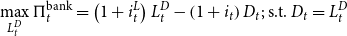 \begin{equation*} \max _{L_{t}^{D}}\Pi _{t}^{\text{bank}}=\left ( 1+i_{t}^{L}\right ) L_{t}^{D}-\left ( 1+i_{t}\right ) D_{t};\ \text {s.t. }D_{t}=L_{t}^{D} \end{equation*}
and the optimality condition implies: $i_{t}^{L}=i_{t}$
.
$i_{t}^{L}=i_{t}$
.
Being $D_{t}=L_{t}^{D}=L_{t}^{S}$
, it follows that the borrowing constraint—which we here assume to hold with equality—can be written as
$D_{t}=L_{t}^{D}=L_{t}^{S}$
, it follows that the borrowing constraint—which we here assume to hold with equality—can be written as
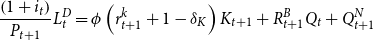 \begin{equation} \frac{\left ( 1+i_{t}\right ) }{P_{t+1}}L_{t}^{D}=\phi \left ( r_{t+1}^{k}+1-\delta _{K}\right ) K_{t+1}+R_{t+1}^{B}Q_{t}+Q_{t+1}^{N} \end{equation}
The optimization problem of the borrowers is
 \begin{equation} \max _{I_{t},L_{t}^{D_{\text{real}}},Q_{t},Q_{t+1}^{N},S_{t+1}}\mathcal{U}^{b}\,\text{s.t. (G12), (G13), (G15)} \end{equation}
If the collateral constraint always holds, by using equation (G15) the demand for credit funds, rewritten with the appropriate expectation operators, will be:
 \begin{equation} L_{t}^{D_{\text{real}}}=\frac{1}{\mathbb{E}_{t}R_{t+1}}\left [ \phi \mathbb{E}_{t}\left ( r_{t+1}^{k}K_{t+1}\right ) +\phi \left ( 1-\delta _{K}\right ) K_{t+1}+\mathbb{E}_{t}Q_{t+1}\right ] \end{equation}
Then, the first-order conditions of equation (G16) deliver the equilibrium condition in asset (and credit) markets:
 \begin{equation} \mathbb{E}_{t}R_{t+1}^{B}=\mathbb{E}_{t}R_{t+1} \end{equation}
and in investments:
 \begin{equation} K_{t+1}=\frac{\beta ^{\frac{1}{\gamma _{b}}}\left ( L_{t}^{D_{\text{real}}}-Q_{t}+S_{t}\right ) +\left [ \left ( 1-\phi \right ) \left ( \mathbb{E}_{t}R_{t}^{K}\right ) \right ] ^{-\frac{1}{\gamma _{b}}}S_{t+1}}{\beta ^{\frac{1}{\gamma _{b}}}+\left [ \left ( 1-\phi \right ) \left ( \mathbb{E}_{t}R_{t}^{K}\right ) \right ] ^{1-\frac{1}{\gamma _{b}}}} \end{equation}
where the return factor is $R_{t}^{K}=r_{t}^{k}+1-\delta _{K}$
. The latter implies that:
$R_{t}^{K}=r_{t}^{k}+1-\delta _{K}$
. The latter implies that:
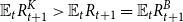 \begin{equation*} \mathbb {E}_{t}R_{t+1}^{K}\gt \mathbb {E}_{t}R_{t+1}=\mathbb {E}_{t}R_{t+1}^{B} \end{equation*}
which must be satisfied in equilibrium.Footnote 30
Finally, the first-order condition of (G16) with respect to $S_{t+1}$
(recall that
$S_{t+1}$
(recall that $S_{t}$
is predetermined for the young agent) leads to:
$S_{t}$
is predetermined for the young agent) leads to:
 \begin{equation*} S_{t}=\left ( 1-\phi \right ) \left [ 1+\left ( \frac {\beta }{\eta }\right ) ^{\frac {1}{\gamma _{b}}}\right ] ^{-1}R_{t}^{K}K_{t} \end{equation*}
that is, the amount of the bequest is proportional to the net resources $R_{t}^{K}K_{t}$
deriving from capital ownership.
$R_{t}^{K}K_{t}$
deriving from capital ownership.
G.3. Intermediate and final firms
Intermediate firm. The firm’s production technology is of the Cobb–Douglas type:
 \begin{equation} X_{t}=F\left ( K_{t};\,N_{t}\right ) =AK_{t}^{\alpha }\left ( g^{t}N_{t}\right ) ^{1-\alpha };\quad \alpha \in \left ( 0;\,1\right ) \end{equation}
where $A\gt 0$
is a scale factor. We assume that the economy grows at rate
$A\gt 0$
is a scale factor. We assume that the economy grows at rate $g\gt 1$
, according to an exogenous (Harrod-neutral) technical progress. The intermediate firm profit, expressed in real terms, is
$g\gt 1$
, according to an exogenous (Harrod-neutral) technical progress. The intermediate firm profit, expressed in real terms, is
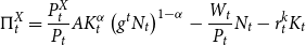 \begin{equation*} \Pi _{t}^{X}=\frac {P_{t}^{X}}{P_{t}}AK_{t}^{\alpha }\left ( g^{t}N_{t}\right ) ^{1-\alpha }-\frac {W_{t}}{P_{t}}N_{t}-r_{t}^{k}K_{t} \end{equation*}
where $P_{t}^{X}/P_{t}$
is the real price of the intermediate good. The demand functions for inputs stemming from profit maximization (with
$P_{t}^{X}/P_{t}$
is the real price of the intermediate good. The demand functions for inputs stemming from profit maximization (with $N_{t}=1$
) are as follows:
$N_{t}=1$
) are as follows:
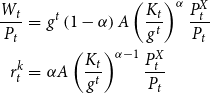 \begin{eqnarray*} \frac{W_{t}}{P_{t}} &=&g^{t}\left ( 1-\alpha \right ) A\left ( \frac{K_{t}}{g^{t}}\right ) ^{\alpha }\frac{P_{t}^{X}}{P_{t}} \\ r_{t}^{k} &=&\alpha A\left ( \frac{K_{t}}{g^{t}}\right ) ^{\alpha -1}\frac{P_{t}^{X}}{P_{t}} \end{eqnarray*}
Final goods producers. The production function of the $j\text{th}$
producer is linear in the input
$j\text{th}$
producer is linear in the input $X_{t}\left ( j\right )$
:
$X_{t}\left ( j\right )$
:
 \begin{equation} Y_{t}\left ( j\right ) =X_{t}\left ( j\right ) \end{equation}
and the monopolist faces a demand:
 \begin{equation} Y_{t}\left ( j\right ) =\left ( \frac{P_{t}\left ( j\right ) }{P_{t}}\right ) ^{-\epsilon }\left ( C_{t}+I_{t}\right ), \quad \text{where }C_{t}\equiv C_{1,t}^{b}+C_{2,t}^{b}+C_{1,t}^{s}+C_{2,t}^{s} \end{equation}
The final producer’s real profit is $\Pi ^{R}\left ( j\right ) _{t}=\frac{P_{t}\left ( j\right ) }{P_{t}}Y_{t}\left ( j\right ) -\frac{P_{t}^{X}}{P_{t}}X_{t}\left ( j\right )$
, where
$\Pi ^{R}\left ( j\right ) _{t}=\frac{P_{t}\left ( j\right ) }{P_{t}}Y_{t}\left ( j\right ) -\frac{P_{t}^{X}}{P_{t}}X_{t}\left ( j\right )$
, where $\frac{P_{t}^{X}}{P_{t}}X_{t}\left ( j\right )$
is the real cost of production. Hence, the firm’s marginal cost is
$\frac{P_{t}^{X}}{P_{t}}X_{t}\left ( j\right )$
is the real cost of production. Hence, the firm’s marginal cost is $mc_{t}=\frac{P_{t}^{X}}{P_{t}}$
. The monopolist sets the price
$mc_{t}=\frac{P_{t}^{X}}{P_{t}}$
. The monopolist sets the price $P_{t}^{o}\left ( j\right )$
so as to solve the problem:
$P_{t}^{o}\left ( j\right )$
so as to solve the problem:
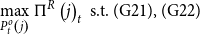 \begin{equation*} \max _{P_{t}^{o}\left ( j\right ) }\Pi ^{R}\left ( j\right ) _{t} \text{ s.t. (G21), (G22)} \end{equation*}
Hence, the real price of the individual good $j$
writes:
$j$
writes:
 \begin{equation} \frac{P_{t}^{o}\left ( j\right ) }{P_{t}}=\left ( \frac{\epsilon }{\epsilon -1}\right ) mc_{t}. \end{equation}
As we assume nominal rigidities, in every $t$
, some of the prices
$t$
, some of the prices $P_{t}^{o}\left ( j\right )$
can be equal to a value set some period in the past. We may hence assume that the average price index
$P_{t}^{o}\left ( j\right )$
can be equal to a value set some period in the past. We may hence assume that the average price index $P_{t}$
is a function not only of the current
$P_{t}$
is a function not only of the current $mc_{t}$
but also of the level of prices and marginal cost that were expected in the past:Footnote
31
$mc_{t}$
but also of the level of prices and marginal cost that were expected in the past:Footnote
31
 \begin{equation} P_{t}=P\left ( mc_{t};\,\mathbb{E}_{t-1-s}P_{t};\,\mathbb{E}_{t-1-s}mc_{t}\right ) _{s=0,1,2\ldots,\infty } \end{equation}
Under a flexible price regime in which $P_{t}^{o}\left ( j\right ) =P_{t}$
, equation (G23) univocally sets the value of the marginal cost
$P_{t}^{o}\left ( j\right ) =P_{t}$
, equation (G23) univocally sets the value of the marginal cost $mc_{t}=\mu =1-\frac{1}{\epsilon }\in \left ( 0;\,1\right )$
,
$mc_{t}=\mu =1-\frac{1}{\epsilon }\in \left ( 0;\,1\right )$
, $\forall t$
, where
$\forall t$
, where $\frac{1}{\mu }$
is the mark-up over production costs.
$\frac{1}{\mu }$
is the mark-up over production costs.
G.4. Monetary policy
In order to calculate the predicted dynamic responses of the model economy to an exogenous shock to the nominal interest rate ( $i_{t}$
), we assume that the monetary authority sets the policy rate according to equation (5), discussed in the main text.
$i_{t}$
), we assume that the monetary authority sets the policy rate according to equation (5), discussed in the main text.
G.5. Stationary state
The economy converges to one unique steady state, where the endogenous model variables are constant through time, and prices are fully flexible, so that $P\left ( j\right ) =P,$ $mc=\mu$
and
$mc=\mu$
and $y\left ( j\right ) =y=\int _{0}^{1}y\left ( j\right ) dj=\bar{y}=x$
, zero trend inflation is assumed:
$y\left ( j\right ) =y=\int _{0}^{1}y\left ( j\right ) dj=\bar{y}=x$
, zero trend inflation is assumed: $\pi =0$
, and the bubble-to-output share is at its ergodic level,
$\pi =0$
, and the bubble-to-output share is at its ergodic level, $\omega =\bar{\omega }$
.Footnote
32
The latter is equal to the weighted average of the two state-specific shares
$\omega =\bar{\omega }$
.Footnote
32
The latter is equal to the weighted average of the two state-specific shares $\omega ^{mf}$
, where the weights are the ergodic states’ probabilities.
$\omega ^{mf}$
, where the weights are the ergodic states’ probabilities.
The equilibrium system can be reduced to the following set of equations:
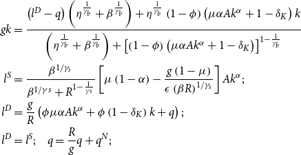 \begin{align} gk &=\frac{\left ( l^{D}-q\right ) \left ( \eta ^{\frac{1}{\gamma _{b}}}+\beta ^{\frac{1}{\gamma _{b}}}\right ) +\eta ^{\frac{1}{\gamma _{b}}}\left ( 1-\phi \right ) \left ( \mu \alpha Ak^{\alpha }+1-\delta _{K}\right ) k}{\left ( \eta ^{\frac{1}{\gamma _{b}}}+\beta ^{\frac{1}{\gamma _{b}}}\right ) +\left [ \left ( 1-\phi \right ) \left ( \mu \alpha Ak^{\alpha }+1-\delta _{K}\right ) \right ] ^{1-\frac{1}{\gamma _{b}}}} \\ l^{S} &=\frac{\beta ^{1/\gamma _{s}}}{\beta ^{1/\gamma s}+R^{1-\frac{1}{\gamma s}}}\left [ \mu \left ( 1-\alpha \right ) -\frac{g\left ( 1-\mu \right ) }{\epsilon \left ( \beta R\right ) ^{1/\gamma _{s}}}\right ] Ak^{\alpha }; \notag \\ l^{D} &=\frac{g}{R}\left ( \phi \mu \alpha Ak^{\alpha }+\phi \left ( 1-\delta _{K}\right ) k+q\right ) ; \notag \\ l^{D} &=l^{S}; \quad q=\frac{R}{g}q+q^{N}; \notag \end{align}
By assuming $\bar{\omega }\gt 0$
, which requires
$\bar{\omega }\gt 0$
, which requires $\omega ^{mf}\neq 0$
at least in one state, the economy is in a bubbly stationary equilibrium, i.e., a vector
$\omega ^{mf}\neq 0$
at least in one state, the economy is in a bubbly stationary equilibrium, i.e., a vector $\left ( l^{D},l^{S},k,R,q\right )$
solves (G25) under
$\left ( l^{D},l^{S},k,R,q\right )$
solves (G25) under $q^{N}\gt 0$
, where the bubble market
$q^{N}\gt 0$
, where the bubble market $q=\left ( \frac{g}{g-R}\right ) q^{N}$
poses a constraint: given
$q=\left ( \frac{g}{g-R}\right ) q^{N}$
poses a constraint: given $q^{N}\geq 0$
, the interest rate on the credit (and the bubble) market must be small enough:
$q^{N}\geq 0$
, the interest rate on the credit (and the bubble) market must be small enough: $g\gt R=R^{B}$
. This condition is necessary for the young agents to be able to buy the bubble (using their resources and the lent funds).
$g\gt R=R^{B}$
. This condition is necessary for the young agents to be able to buy the bubble (using their resources and the lent funds).
From the equilibrium $l^{D}=l^{S}$
we obtain:
$l^{D}=l^{S}$
we obtain:
 \begin{align} \phi \left ( 1-\delta _{K}\right ) =\left \{ \frac{\beta ^{1/\gamma _{s}}}{\beta ^{1/\gamma s}/R+R^{-\frac{1}{\gamma s}}}\left [ \frac{\mu \left (1-\alpha \right ) }{g}-\frac{1}{\epsilon \left ( \beta R\right ) ^{1/\gamma _{s}}}\right ] -\phi \mu \alpha -\frac{\bar{\omega } g}{g-R}\right \} Ak^{\alpha -1} \end{align}
Furthermore, as we also assume that $\gamma _{b}=1$
, the borrowers’ accumulation equation is
$\gamma _{b}=1$
, the borrowers’ accumulation equation is
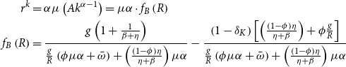 \begin{align} r^{k} &=\alpha \mu \left ( Ak^{\alpha -1}\right ) =\mu \alpha \cdot f_{B}\left ( R\right ) \\ f_{B}\left ( R\right ) &=\frac{g\left ( 1+\frac{1}{\beta +\eta }\right ) }{\frac{g}{R}\left ( \phi \mu \alpha +\bar{\omega } \right ) +\left ( \frac{\left ( 1-\phi \right ) \eta }{\eta +\beta }\right ) \mu \alpha }-\frac{\left ( 1-\delta _{K}\right ) \left [ \left ( \frac{\left ( 1-\phi \right ) \eta }{\eta +\beta }\right ) +\phi \frac{g}{R}\right ] }{\frac{g}{R}\left ( \phi \mu \alpha +\bar{\omega } \right ) +\left ( \frac{\left ( 1-\phi \right ) \eta }{\eta +\beta }\right ) \mu \alpha } \notag \end{align}
H. Model solution method
The Markov-switching OLG model is solved using the perturbation method of Foerster et al. (Reference Foerster, Rubio-Ramirez, Waggoner and Zha2016). They develop an iterative procedure that approximates the model’s solution by guessing a set of approximations under each regime; on this basis, each regime’s approximation follows standard perturbation techniques. The iterative algorithm stops when obtained approximations equal the guesses.
We stack the vector of model variables $\Upsilon _t$
into a group of predetermined variables,
$\Upsilon _t$
into a group of predetermined variables, $\textbf{x}_{t}\in \mathbb{R}^{n_x}$
, and a group of control variables,
$\textbf{x}_{t}\in \mathbb{R}^{n_x}$
, and a group of control variables, $\textbf{y}_t\in \mathbb{R}^{n_y}$
. Then, we define the vector of independent and identically distributed innovations to the exogenous predetermined variables as
$\textbf{y}_t\in \mathbb{R}^{n_y}$
. Then, we define the vector of independent and identically distributed innovations to the exogenous predetermined variables as $\epsilon _t\in \mathbb{R}^{n_\epsilon }$
and the vector of switching parameters as
$\epsilon _t\in \mathbb{R}^{n_\epsilon }$
and the vector of switching parameters as $\theta \left(\xi _t^{mf}\right)\in \mathbb{R}^{n_\theta }$
.
$\theta \left(\xi _t^{mf}\right)\in \mathbb{R}^{n_\theta }$
.
The equilibrium conditions have the following general form:
 \begin{equation*} \mathbb {E}_t\textbf {f}\left(\textbf {y}_{t+1}, \textbf {y}_t, \textbf {x}_t, \textbf {x}_{t-1}, \epsilon _{t+1},\epsilon _t, \theta \left(\xi _{t+1}^{mf}\right), \theta \left(\xi _t^{mf}\right) \right)=0_{n_y+n_x} \end{equation*}
where $\textbf{f}$
is a nonlinear function. Then, the algorithm works as an extension of conventional perturbation methods [Judd (Reference Judd1998) and Schmitt-Grohé and Uribe (Reference Schmitt-Grohé and Uribe2004)], where not only
$\textbf{f}$
is a nonlinear function. Then, the algorithm works as an extension of conventional perturbation methods [Judd (Reference Judd1998) and Schmitt-Grohé and Uribe (Reference Schmitt-Grohé and Uribe2004)], where not only $\epsilon _{t+1}$
is perturbed but also the switching parameters,
$\epsilon _{t+1}$
is perturbed but also the switching parameters, $\theta \left(\xi _{t+1}^{mf}\right)$
,
$\theta \left(\xi _{t+1}^{mf}\right)$
, $\theta \left(\xi _t^{mf}\right)$
. Since in our model, the steady state is affected by the policy regime in place, the perturbation function for
$\theta \left(\xi _t^{mf}\right)$
. Since in our model, the steady state is affected by the policy regime in place, the perturbation function for $\theta \left(\xi _t^{mf}\right)$
is
$\theta \left(\xi _t^{mf}\right)$
is $\theta (k,\chi )=\chi \theta (k)+(1-\chi )\bar{\theta }$
, where
$\theta (k,\chi )=\chi \theta (k)+(1-\chi )\bar{\theta }$
, where $\chi \in \mathbb{R}$
is the perturbation parameter,
$\chi \in \mathbb{R}$
is the perturbation parameter, $k$
indicates a generic regime, and
$k$
indicates a generic regime, and $\bar{\theta }=[\theta (1)\ldots \theta (n_\xi )]\bar{p}$
is the ergodic mean of
$\bar{\theta }=[\theta (1)\ldots \theta (n_\xi )]\bar{p}$
is the ergodic mean of $\theta \left(\xi _t^{mf}\right)$
.
$\theta \left(\xi _t^{mf}\right)$
.
Stacking the regime-dependent solutions for $\textbf{y}_t$
and
$\textbf{y}_t$
and $\textbf{x}_t$
, the algorithm assumes they are of the form:
$\textbf{x}_t$
, the algorithm assumes they are of the form:
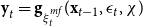 \begin{equation*}\textbf {y}_t=\textbf {g}_{\xi _t^{mf}}(\textbf {x}_{t-1}, \epsilon _t, \chi )\end{equation*}
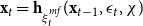 \begin{equation*}\textbf {x}_t=\textbf {h}_{\xi _t^{mf}}(\textbf {x}_{t-1}, \epsilon _t, \chi )\end{equation*}
for all $\xi ^{mf}_t$
, where
$\xi ^{mf}_t$
, where $\textbf{g}_{\xi _t^{mf}}\,:\,\mathbb{R}^{n_x+n_\epsilon +1}\rightarrow \mathbb{R}^{n_y}$
and
$\textbf{g}_{\xi _t^{mf}}\,:\,\mathbb{R}^{n_x+n_\epsilon +1}\rightarrow \mathbb{R}^{n_y}$
and $\textbf{h}_{\xi _t^{mf}}\,:\,\mathbb{R}^{n_x+n_\epsilon +1}\rightarrow \mathbb{R}^{n_x}$
are continuously differentiable regime-dependent functions. Then,
$\textbf{h}_{\xi _t^{mf}}\,:\,\mathbb{R}^{n_x+n_\epsilon +1}\rightarrow \mathbb{R}^{n_x}$
are continuously differentiable regime-dependent functions. Then, $\textbf{Y}_t=y_t\left(\textbf{e}^{T}_{\xi ^{mf}_t}\otimes \textbf{I}_{n_y}\right)^{-1}$
and
$\textbf{Y}_t=y_t\left(\textbf{e}^{T}_{\xi ^{mf}_t}\otimes \textbf{I}_{n_y}\right)^{-1}$
and $\textbf{X}_t=x_t\left(\textbf{e}^{T}_{\xi ^{mf}_t}\otimes \textbf{I}_{n_x}\right)^{-1}$
, such that approximating a solution to
$\textbf{X}_t=x_t\left(\textbf{e}^{T}_{\xi ^{mf}_t}\otimes \textbf{I}_{n_x}\right)^{-1}$
, such that approximating a solution to $\textbf{y}_t$
and
$\textbf{y}_t$
and $\textbf{x}_t$
is equivalent to approximating to:
$\textbf{x}_t$
is equivalent to approximating to:
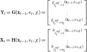 \begin{gather*} \textbf{Y}_t=\textbf{G}(\textbf{x}_{t-1},\epsilon _t,\chi )=\left [ \begin{smallmatrix} g_{\xi _t^{mf}=1}(\textbf{x}_{t-1},\epsilon _t,\chi ) \\[3pt] \vdots \\[3pt] g_{\xi _t^{mf}=n_\xi }(\textbf{x}_{t-1},\epsilon _t,\chi ) \end{smallmatrix}\right ]\\[3pt] \textbf{X}_t=\textbf{H}(\textbf{x}_{t-1},\epsilon _t,\chi )=\left [ \begin{smallmatrix} h_{\xi _t^{mf}=1}(\textbf{x}_{t-1},\epsilon _t,\chi ) \\[3pt] \vdots \\ h_{\xi _t^{mf}=n_\xi }(\textbf{x}_{t-1},\epsilon _t,\chi ) \end{smallmatrix}\right ] \end{gather*}
Given the vector of states $z_t=({x}_{t-1}$
,
$z_t=({x}_{t-1}$
, $\epsilon _t$
,
$\epsilon _t$
, $\xi _t^{mf}$
) of dimension
$\xi _t^{mf}$
) of dimension $n_x+n_{\epsilon }+1$
, the first-order approximation of
$n_x+n_{\epsilon }+1$
, the first-order approximation of $G(z_t)$
and
$G(z_t)$
and $H(z_t)$
is:
$H(z_t)$
is:
 \begin{gather*} \textbf{G}(\textbf{z}_{t})\approx Y+D\textbf{G}\left (\textbf{z}_{\xi ^{mf}_t}\right )\left (\textbf{z}_t-\textbf{z}_{\xi ^{mf}_t}\right )\\ \textbf{H}(\textbf{z}_{t})\approx X+D\textbf{H}\left (\textbf{z}_{\xi ^{mf}_t}\right )\left (\textbf{z}_t-\textbf{z}_{\xi ^{mf}_t}\right )\end{gather*}
where $D\textbf{G}\left (\textbf{z}_{\xi ^{mf}_t}\right )$
and
$D\textbf{G}\left (\textbf{z}_{\xi ^{mf}_t}\right )$
and $D\textbf{H}\left (\textbf{z}_{\xi ^{mf}_t}\right )$
can be obtained by solving a system of quadratic polynomial equations and two systems of linear equations.
$D\textbf{H}\left (\textbf{z}_{\xi ^{mf}_t}\right )$
can be obtained by solving a system of quadratic polynomial equations and two systems of linear equations.


 Open access