


1. Introduction
The motivation behind this paper is the following question: what are the measures $\mu$
on the Heisenberg group
$\mu$
on the Heisenberg group ${\mathbb{H}}^n$
which guarantee that the (correct notion of) Riesz transform is bounded from
${\mathbb{H}}^n$
which guarantee that the (correct notion of) Riesz transform is bounded from $L^{2}(\mu)$
to itself? This question (or some variant of it) with
$L^{2}(\mu)$
to itself? This question (or some variant of it) with $\mathbb{R}^n$
instead of
$\mathbb{R}^n$
instead of ${\mathbb{H}}^n$
, was one of the major starting points of the theory that came to be known as quantitative rectifiability. This area of geometric measure theory has seen an impressive development in the past thirty years, starting with the landmark works of Peter Jones [
Reference JonesJon90
] and David and Semmes [
Reference David and SemmesDS91
], [
Reference David and SemmesDS93
], through the solution of fundamental questions in complex analysis, such as the Painlevé problem (see [
Reference Mattila, Melnikov and VerderaMMV96
], [
Reference DavidDav98
], [
Reference TolsaTol03
]), to more recent applications to harmonic analysis, see for example [
Reference Nazarov, Tolsa and VolbergNTV14
] and [
Reference Azzam, Hofmann, Martell, Mourgoglou and TolsaAHM+19
].
${\mathbb{H}}^n$
, was one of the major starting points of the theory that came to be known as quantitative rectifiability. This area of geometric measure theory has seen an impressive development in the past thirty years, starting with the landmark works of Peter Jones [
Reference JonesJon90
] and David and Semmes [
Reference David and SemmesDS91
], [
Reference David and SemmesDS93
], through the solution of fundamental questions in complex analysis, such as the Painlevé problem (see [
Reference Mattila, Melnikov and VerderaMMV96
], [
Reference DavidDav98
], [
Reference TolsaTol03
]), to more recent applications to harmonic analysis, see for example [
Reference Nazarov, Tolsa and VolbergNTV14
] and [
Reference Azzam, Hofmann, Martell, Mourgoglou and TolsaAHM+19
].
In the last years, there has been an increasing interest in developing such a quantitative theory in different contexts than that of Euclidean spaces; examples of these are parabolic spaces and Heisenberg groups, or, more generally, Carnot groups. The former appear in the study of caloric measure. The latter arise naturally in the study of certain hypoelliptic operators, in the sense that the natural translations and dilations for these operators are those characterising the spaces; the Heisenberg group is the most important prototypical example, and the related operator is the so-called Kohn Laplacian; see [ Reference Bonfiglioli, Lanconelli and UguzzoniBLU07 ] for a comprehensive study of stratified Lie groups and the corresponding operators.
We should mention that the study of Heisenberg geometry can be approached from different perspectives and with different applications in mind; for example, see [ Reference Naor and YoungNY18 ] for a connection with theoretical computer science.
To be a little more specific: the starting motivation to develop a theory of quantitative rectifiability connected to our initial question, is to understand basic issues such as the removable sets for harmonic functions (with respect to the relevant sub-Laplacian), or to give a characterisation of those domains where the Dirichlet problem (again, for the relevant sub-Laplacian) is well-posed. We want to underline, however, that a theory of quantitative rectifiability in the Heisenberg setting has its own, purely geometric, intrinsic appeal.
In the last couple of years, there has been some progress towards an answer to our initial question; see for example [
Reference Chousionis, Fässler and OrponenCFO19
], [
Reference Fässler and OrponenFO18
] and [
Reference OrponenOrp18
]. In this note we give a necessary condition to be imposed on a Radon measure $\mu$
on
$\mu$
on ${\mathbb{H}}^n$
for the Riesz transform to be
${\mathbb{H}}^n$
for the Riesz transform to be $L^2(\mu)$
bounded. Here
$L^2(\mu)$
bounded. Here $R_{\mu}$
is the singular integral operator whose kernel is the horizontal gradient of the fundamental solution of the Heisenberg sub-Laplacian, as defined in [
Reference Chousionis and MattilaCM12
]. See Section 2 for precise definitions.
$R_{\mu}$
is the singular integral operator whose kernel is the horizontal gradient of the fundamental solution of the Heisenberg sub-Laplacian, as defined in [
Reference Chousionis and MattilaCM12
]. See Section 2 for precise definitions.
Theorem 1·1.
Let $\mu$
be a Radon measure on
$\mu$
be a Radon measure on ${\mathbb{H}}^n$
such that
${\mathbb{H}}^n$
such that $R_\mu$
is bounded on
$R_\mu$
is bounded on $L^2(\mu)$
with norm
$L^2(\mu)$
with norm $C_1$
, and such that
$C_1$
, and such that $\mu(F) = 0$
whenever
$\mu(F) = 0$
whenever $\text{dim}_H(F) \leq 2$
. Then there exists a constant
$\text{dim}_H(F) \leq 2$
. Then there exists a constant $C_2$
such that for all balls
$C_2$
such that for all balls $B(x,r) \subset {\mathbb{H}}^n$
, we have
$B(x,r) \subset {\mathbb{H}}^n$
, we have
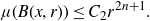 \begin{align} \mu(B(x,r)) \leq C_2 r^{2n +1}.\end{align}
Here $C_2$
depends only on n and
$C_2$
depends only on n and $C_1$
, and the ball B(x,r) is defined with respect to the Korányi metric, see Section 2.
$C_1$
, and the ball B(x,r) is defined with respect to the Korányi metric, see Section 2.
A corresponding statement holds in the Euclidean setting, and is a result of David, [
Reference DavidDav91
part III, proposition 1·4]. See [
Reference OrponenOrp17
, proposition 6·9] for a more detailed proof. Let $\mathcal{R}^{d}_\mu$
denote the standard d-dimensional Riesz transform in
$\mathcal{R}^{d}_\mu$
denote the standard d-dimensional Riesz transform in $\mathbb{R}^n$
.
$\mathbb{R}^n$
.
Theorem 1·2.
Assume that $\mu$
is a non-atomic Radon measure on
$\mu$
is a non-atomic Radon measure on $\mathbb{R}^n$
such that
$\mathbb{R}^n$
such that $\mathcal{R}^{d}_\mu$
is bounded on
$\mathcal{R}^{d}_\mu$
is bounded on $L^2(\mu)$
with norm
$L^2(\mu)$
with norm $C_1$
. Then, for all Euclidean balls
$C_1$
. Then, for all Euclidean balls $B_{\mathbb{R}^n}(x,r)\subset\mathbb{R}^n$
we have
$B_{\mathbb{R}^n}(x,r)\subset\mathbb{R}^n$
we have
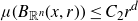 \begin{align}\mu (B_{\mathbb{R}^n}(x,r)) \leq C_2 r^d\end{align}
Here $C_2$
depends only on
$C_2$
depends only on $C_1$
, n, and d.
$C_1$
, n, and d.
A measure satisfying (1·2) (or (1·1)) is said to have polynomial growth. Let us give a couple of remarks.
Remark 1·3. Although the result itself (both in the Euclidean and Heisenberg case) is neither hard nor deep, it is nevertheless very useful. For example, most tools developed in the last two decades that take quantitative rectifiability beyond Ahlfors regular measures still need polynomial growthFootnote 1 (see for example the book by Tolsa [ Reference TolsaTol14 ]). Thus, we expect that our result will be quite useful, too.
Remark 1·4. While the two results above look similar, there is actually a difference, in the sense that, in the Heisenberg case, there actually exist lower dimensional measures which give a bounded Riesz transform, but are not atomic.
This is not a byproduct of the proof, but rather a fact of the Heisenberg geometry. Indeed, the 2-dimensional t-axis (or any Heisenberg translate of it) gives a bounded $(2n+1)$
-dimensional Riesz transform; this is simply because on these sets the kernel vanishes identically, see (2·4).
$(2n+1)$
-dimensional Riesz transform; this is simply because on these sets the kernel vanishes identically, see (2·4).
One can construct a more interesting example in the vertical plane of the one dimensional Heisenberg group ${\mathbb{H}}$
, say. Consider a tube of height 1 and radius
${\mathbb{H}}$
, say. Consider a tube of height 1 and radius $\varepsilon_1^2$
around the t-axis, and take the intersection with the vertical plane. Call the resulting rectangle
$\varepsilon_1^2$
around the t-axis, and take the intersection with the vertical plane. Call the resulting rectangle $R_{1,1}$
. Cut out from
$R_{1,1}$
. Cut out from $R_1$
two smaller rectangles
$R_1$
two smaller rectangles $R_{2,1}$
and
$R_{2,1}$
and $R_{2,2}$
, one in the top right corner and one in the bottom left corner, both of height
$R_{2,2}$
, one in the top right corner and one in the bottom left corner, both of height $\varepsilon_2$
and width
$\varepsilon_2$
and width $\varepsilon_2^2$
, for some
$\varepsilon_2^2$
, for some $\varepsilon_2\le \varepsilon_1/4$
. We proceed in this way, so that after k steps we have
$\varepsilon_2\le \varepsilon_1/4$
. We proceed in this way, so that after k steps we have $2^{k-1}$
disjoint rectangles
$2^{k-1}$
disjoint rectangles $\{R_{k,i}\}_i$
of height
$\{R_{k,i}\}_i$
of height $\varepsilon_k$
and width
$\varepsilon_k$
and width $\varepsilon_k^2$
. Consider the natural probability measure
$\varepsilon_k^2$
. Consider the natural probability measure $\mu$
on the Cantor-like set
$\mu$
on the Cantor-like set $C=\bigcap_k\bigcup_i R_{k,i}$
. It is not difficult to show that, if
$C=\bigcap_k\bigcup_i R_{k,i}$
. It is not difficult to show that, if $\varepsilon_k\to 0$
are small enough, the Heisenberg Riesz transform is bounded on
$\varepsilon_k\to 0$
are small enough, the Heisenberg Riesz transform is bounded on $L^2(\mu)$
; the idea is that the set is concentrated along the t-axis, and thus the kernel is very small (see (2·4) below). Depending on the choice of
$L^2(\mu)$
; the idea is that the set is concentrated along the t-axis, and thus the kernel is very small (see (2·4) below). Depending on the choice of $(\varepsilon_k)$
we have
$(\varepsilon_k)$
we have $\text{dim}_H(C)\in [0,2].$
Organisation of the paper. In Section 2 we briefly recall basic facts about Heisenberg groups and the Riesz transform. We also introduce a family of “dyadic cubes” suitable to our setting.
Section 3 is dedicated to Lemma 3·1, our main technical lemma. Roughly speaking, we show that if a measure $\mu$
is such that
$\mu$
is such that $R_{\mu}$
is bounded on
$R_{\mu}$
is bounded on $L^2(\mu)$
, and there is some cube
$L^2(\mu)$
, and there is some cube $Q_0$
with a very high concentration of
$Q_0$
with a very high concentration of $\mu$
(i.e.
$\mu$
(i.e. $\mu(Q_0)\gg \ell(Q_0)^{2n+1}$
), then we can find a family
$\mu(Q_0)\gg \ell(Q_0)^{2n+1}$
), then we can find a family ${\mathsf{HD}}(Q_0)$
of much smaller cubes, contained in
${\mathsf{HD}}(Q_0)$
of much smaller cubes, contained in $Q_0$
, such that:
$Q_0$
, such that:
-
(a) a very large portion of measure $\mu$
on
$Q_0$
is concentrated on the cubes from
${\mathsf{HD}}(Q_0)$
;
$\mu$
on
$Q_0$
is concentrated on the cubes from
${\mathsf{HD}}(Q_0)$
; -
(b) the family
${\mathsf{HD}}(Q_0)$
is relatively small, in the sense that it consists of few cubes.


In Section 4 we show that if the polynomial growth condition (1·1) is not satisfied, then we can find a cube satisfying the assumptions of our main lemma. This in turn allows us to start an iteration algorithm, consisting of using the main lemma countably many times, that results in constructing a set Z with $\mu(Z)>0$
and
$\mu(Z)>0$
and $\text{dim}_H(Z)\le 2.$
This completes the proof of Theorem 1·1.
$\text{dim}_H(Z)\le 2.$
This completes the proof of Theorem 1·1.
2. Preliminaries
In our estimates we will often use the notation $f\lesssim g$
which means that there exists some absolute constant C for which
$f\lesssim g$
which means that there exists some absolute constant C for which $f\le Cg.$
If the constant C depends on some parameter t, we will write
$f\le Cg.$
If the constant C depends on some parameter t, we will write $f\lesssim_t g.$
Notation
$f\lesssim_t g.$
Notation $f\approx g$
will stand for
$f\approx g$
will stand for $f\lesssim g\lesssim f,$
and
$f\lesssim g\lesssim f,$
and $f\approx_t g$
is defined analogously. For simplicity, in our estimates we will suppress the dependence on dimension n and on absolute constant
$f\approx_t g$
is defined analogously. For simplicity, in our estimates we will suppress the dependence on dimension n and on absolute constant $\lambda,\ \Lambda$
(see (2·7)).
$\lambda,\ \Lambda$
(see (2·7)).
2·1. Heisenberg group
In this paper we consider the nth Heisenberg group with exponential coordinates (see [
Reference Capogna, Danielli, Pauls and TysonCDPT07
] or [
Reference FässlerFas19
] for a swift introduction to the Heisenberg group in a context close to ours). In practice, we will denote a point $p \in {\mathbb{H}}^n$
as
$p \in {\mathbb{H}}^n$
as $(z,t) \in \mathbb{R}^{2n} \times \mathbb{R}$
, and
$(z,t) \in \mathbb{R}^{2n} \times \mathbb{R}$
, and $z=(x_1,...,x_n,y_1,...,y_n)$
. In these coordinates the group law in
$z=(x_1,...,x_n,y_1,...,y_n)$
. In these coordinates the group law in ${\mathbb{H}}^n$
takes the form
${\mathbb{H}}^n$
takes the form
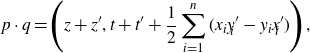 \begin{align*} p \cdot q = \left( z + z', t+t' + \frac{1}{2} \sum_{i=1}^n (x_i y'_{\!\!i} - y_i x'_{\!\!i}) \right),\end{align*}
where $p=(z,t)$
and
$p=(z,t)$
and $q=(z',t')$
. The identity element is the origin (0,0) and the inverse is given by
$q=(z',t')$
. The identity element is the origin (0,0) and the inverse is given by $p^{-1}=(\!-\!z,-t)$
. We make
$p^{-1}=(\!-\!z,-t)$
. We make ${\mathbb{H}}^n$
into a metric space by setting
${\mathbb{H}}^n$
into a metric space by setting $ d(p,q) \;:\!=\; \|q^{-1}\cdot p\|_{\mathbb{H}}$
, where
$ d(p,q) \;:\!=\; \|q^{-1}\cdot p\|_{\mathbb{H}}$
, where
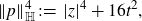 \begin{align} \|p\|_{\mathbb{H}}^4 \;:\!=\; |z|^4 + 16t^2,\end{align}
and $|z|$
denotes the Euclidean norm of
$|z|$
denotes the Euclidean norm of $z\in\mathbb{R}^{2n}$
.
$z\in\mathbb{R}^{2n}$
.
Note that $\|\!\cdot\!\|_{\mathbb{H}}$
is 1-homogeneous with respect to the anisotropic dilation
$\|\!\cdot\!\|_{\mathbb{H}}$
is 1-homogeneous with respect to the anisotropic dilation $p \mapsto \lambda p = (\lambda z, \lambda^2 t)$
,
$p \mapsto \lambda p = (\lambda z, \lambda^2 t)$
, $\lambda >0$
. The metric d is sometimes called the Korányi metric.
$\lambda >0$
. The metric d is sometimes called the Korányi metric.
Given $p\in{\mathbb{H}}^n$
and
$p\in{\mathbb{H}}^n$
and $r>0$
we set
$r>0$
we set
 \begin{equation*} B(p,r)=\left\{q\ |\ d(p,q)\le r \right\},\quad U(p,r) = \left\{q\ |\ d(p,q)< r \right\}.\end{equation*}
For $\alpha>0$
we will write
$\alpha>0$
we will write $\mathcal{H}^{\alpha}$
to denote the usual
$\mathcal{H}^{\alpha}$
to denote the usual $\alpha$
-dimensional Hausdorff measure with respect to metric d. For
$\alpha$
-dimensional Hausdorff measure with respect to metric d. For $A\subset{\mathbb{H}}^n$
we set
$A\subset{\mathbb{H}}^n$
we set $\text{dim}_H(A)$
to be the Hausdorff dimension of A.
$\text{dim}_H(A)$
to be the Hausdorff dimension of A.
It follows easily from the definition of the Korányi metric that for all $p\in{\mathbb{H}}^n$
and
$p\in{\mathbb{H}}^n$
and $r>0$
we have
$r>0$
we have
 \begin{equation} \mathcal{H}^{2n+2}(B(p,r)) = \mathcal{H}^{2n+2}(B(0,1))\, r^{2n+2}.\end{equation}
Thus, even though the topological dimension of ${\mathbb{H}}^n$
is
${\mathbb{H}}^n$
is $2n+1$
, the Hausdorff dimension of
$2n+1$
, the Hausdorff dimension of ${\mathbb{H}}^n$
is equal to
${\mathbb{H}}^n$
is equal to $2n+2$
. For the sake of brevity we set
$2n+2$
. For the sake of brevity we set $D\;:\!=\;2n+2.$
Usually one denotes the Hausdorff dimension of
$D\;:\!=\;2n+2.$
Usually one denotes the Hausdorff dimension of ${\mathbb{H}}^n$
by Q, but we have decided to save that letter for cubes; hence the non-standard notation.
${\mathbb{H}}^n$
by Q, but we have decided to save that letter for cubes; hence the non-standard notation.
It is also easy to check that if $\mathcal{L}^{2n+1}$
denotes the usual Lebesgue measure on
$\mathcal{L}^{2n+1}$
denotes the usual Lebesgue measure on $\mathbb{R}^{2n+1}\simeq {\mathbb{H}}^n,$
then we have a constant
$\mathbb{R}^{2n+1}\simeq {\mathbb{H}}^n,$
then we have a constant $C>0$
such that
$C>0$
such that
 \begin{equation} \mathcal{L}^{2n+1}=C\mathcal{H}^{D}.\end{equation}
2·2. Heisenberg Riesz transform
Recall that, for a function $u \;:\; {\mathbb{H}}^n \to \mathbb{R}$
, the horizontal gradient of u is given by
$u \;:\; {\mathbb{H}}^n \to \mathbb{R}$
, the horizontal gradient of u is given by
 \begin{align*} \nabla_{\mathbb{H}} u \;:\!=\; \left( X_1 u,...,X_n u, Y_1 u, ..., Y_n u \right),\end{align*}
where the vector fields $X_1,\dots,X_n,Y_1,\dots, Y_n$
and
$X_1,\dots,X_n,Y_1,\dots, Y_n$
and ${\partial}/{\partial t}$
represent the left invariant translates of the canonical basis at the identity. In particular,
${\partial}/{\partial t}$
represent the left invariant translates of the canonical basis at the identity. In particular, $X_1,\dots,X_n,Y_1,\dots, Y_n$
span the horizontal distribution in
$X_1,\dots,X_n,Y_1,\dots, Y_n$
span the horizontal distribution in ${\mathbb{H}}^n$
.
${\mathbb{H}}^n$
.
The Heisenberg sublaplacian $\Delta_{\mathbb{H}}$
is given by
$\Delta_{\mathbb{H}}$
is given by $\sum_{i=1}^n X_i^2 + Y_i^2$
, and its fundamental solution is
$\sum_{i=1}^n X_i^2 + Y_i^2$
, and its fundamental solution is
 \begin{align*} G(p) \;:\!=\; c_n \|p\|_{\mathbb{H}}^{2-D}.\end{align*}
The $(D-1)$
-dimensional Riesz kernel in
$(D-1)$
-dimensional Riesz kernel in ${\mathbb{H}}^n$
, first considered in [
Reference Chousionis and MattilaCM12
], is given by
${\mathbb{H}}^n$
, first considered in [
Reference Chousionis and MattilaCM12
], is given by $K(p)=\nabla_{{\mathbb{H}}} G(p).$
The Riesz transform is formally defined as
$K(p)=\nabla_{{\mathbb{H}}} G(p).$
The Riesz transform is formally defined as
 \begin{align*} R_\mu f (p) = \int_{\mathbb{H}^n} K(q^{-1}\cdot p)f(q) \, d\mu(q).\end{align*}
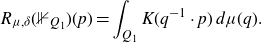
Since it is not clear whether the integral above converges, one considers the truncated Riesz transform given by the formula
 \begin{align*} R_{\mu, \delta}f(p)= \int_{{\mathbb{H}}^n \setminus B(p,\delta)} K(q^{-1}\cdot p)f(q)\ d\mu(q),\end{align*}
for $\delta>0$
. We say that
$\delta>0$
. We say that $R_{\mu}$
is bounded on
$R_{\mu}$
is bounded on $L^2(\mu)$
if the truncated operators
$L^2(\mu)$
if the truncated operators $R_{\mu, \delta}$
are bounded on
$R_{\mu, \delta}$
are bounded on $L^2(\mu)$
uniformly in
$L^2(\mu)$
uniformly in $\delta>0.$
One can easily check that the Riesz kernel is actually equal to
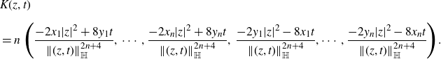 \begin{align*} & K(z, t) \\[5pt] & = n\, \left( \frac{ -2x_1 |z|^2 + 8y_1 t }{\|(z,t)\|_{\mathbb{H}}^{2n+4 }}, \,\cdots , \frac{ -2x_n |z|^2 + 8y_n t }{\|(z,t)\|_{\mathbb{H}}^{2n+4 }}, \, \frac{ -2y_1 |z|^2 - 8x_1 t }{\|(z,t)\|_{\mathbb{H}}^{2n+4}}, \cdots , \frac{ -2y_n |z|^2 - 8x_n t }{\|(z,t)\|_{\mathbb{H}}^{2n+4}} \right).\end{align*}
Hence,
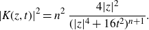 \begin{align} |K(z,t)|^2 = n^2 \, \frac{ 4 |z|^2 }{(|z|^4 + 16t^2)^{n+1}}.\end{align}
This implies the curious fact that $|K(z,t)| \leq C$
whenever
$|K(z,t)| \leq C$
whenever
 \begin{align} |z| \leq \, 16 |t|^{n+1},\end{align}
which is a ‘paraboloidal’ double cone around t-axis with vertex at the origin. This fact will play a key role in the subsequent analysis.
Chousionis and Mattila showed in [
Reference Chousionis and MattilaCM12
, proposition 3·11] that the Riesz kernel is a standard kernel. In particular, it satisfies the following continuity property: whenever $q_1, q_2\neq p\in {\mathbb{H}}^n$
, we have
$q_1, q_2\neq p\in {\mathbb{H}}^n$
, we have
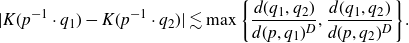 \begin{equation*} |K(p^{-1}\cdot q_1) - K(p^{-1}\cdot q_2)| \lesssim \max\bigg\{\frac{d(q_1,q_2)}{d(p,q_1)^{D}},\frac{d(q_1,q_2)}{d(p,q_2)^{D}} \bigg\}.\end{equation*}
Taking $p=0$
and
$p=0$
and $q_1 = \tilde{q_1}^{-1}\cdot \tilde{p},\ q_2 = \tilde{q_2}^{-1}\cdot \tilde{p},$
one gets immediately that for all
$q_1 = \tilde{q_1}^{-1}\cdot \tilde{p},\ q_2 = \tilde{q_2}^{-1}\cdot \tilde{p},$
one gets immediately that for all $\tilde{q_1}, \tilde{q_2}\neq \tilde{p}\in {\mathbb{H}}^n$
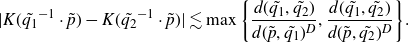 \begin{equation} |K(\tilde{q_1}^{-1}\cdot \tilde{p}) - K(\tilde{q_2}^{-1}\cdot \tilde{p})| \lesssim \max\bigg\{\frac{d(\tilde{q_1},\tilde{q_2})}{d(\tilde{p},\tilde{q_1})^{D}},\frac{d(\tilde{q_1},\tilde{q_2})}{d(\tilde{p},\tilde{q_2})^{D}} \bigg\}.\end{equation}
2·3. Dyadic cubes
We are going to use a family of decompositions of ${\mathbb{H}}^n$
into subsets that share many properties with the standard dyadic cubes from
${\mathbb{H}}^n$
into subsets that share many properties with the standard dyadic cubes from $\mathbb{R}^n$
. The most classical constructions of this kind are due to Christ [
Reference ChristChr90
] and David [
Reference DavidDav88
], but for us it will be more convenient to use the “cubes” constructed in [
Reference Käenmäki, Rajala and SuomalaKRS12
].
$\mathbb{R}^n$
. The most classical constructions of this kind are due to Christ [
Reference ChristChr90
] and David [
Reference DavidDav88
], but for us it will be more convenient to use the “cubes” constructed in [
Reference Käenmäki, Rajala and SuomalaKRS12
].
First, note that given any ball B(p, 2r), one may use the 5r-covering lemma and the property (2·2) to conclude that there exists some absolute constant m such that B(p, 2r) may be covered by m balls $B(p_i,r)$
, where
$B(p_i,r)$
, where $\left\{p_i \right\}_{i=1}^m$
are points in B(p, 2r). That is,
$\left\{p_i \right\}_{i=1}^m$
are points in B(p, 2r). That is, ${\mathbb{H}}^n$
is geometrically doubling. In particular, we can use [
Reference Käenmäki, Rajala and SuomalaKRS12
, theorem 2·1, remark 2·2].
${\mathbb{H}}^n$
is geometrically doubling. In particular, we can use [
Reference Käenmäki, Rajala and SuomalaKRS12
, theorem 2·1, remark 2·2].
Lemma 2·1 ([
Reference Käenmäki, Rajala and SuomalaKRS12
]). For all $k\in\mathbb{Z}$
there exists a family of subsets of
$k\in\mathbb{Z}$
there exists a family of subsets of ${\mathbb{H}}^n$
, denoted by
${\mathbb{H}}^n$
, denoted by $\mathcal{D}_k$
, such that:
$\mathcal{D}_k$
, such that:
-
(i)
${\mathbb{H}}^n = \bigcup_{Q\in\mathcal{D}_k}Q$
; -
(ii) if
$k\ge l$
, and
$Q\in \mathcal{D}_k,\ P\in\mathcal{D}_l$
, then either
$Q\cap P=\varnothing$
or
$Q\subset P$
; -
(iii) for every
$Q\in \mathcal{D}_k$
there exists
$p_Q\in Q$
such that
(2·7)for some absolute constants
\begin{equation} U(p_Q,\lambda2^{-k})\subset Q\subset B(p_Q,\Lambda2^{-k}) \end{equation}
$\lambda,\Lambda>0$
.


Let us stress once more that we will not keep track of how various parameters appearing in the proof depend on $\lambda$
and
$\lambda$
and $\Lambda$
.
$\Lambda$
.
We set $\mathcal{D} = \bigcup_k \mathcal{D}_k$
. For
$\mathcal{D} = \bigcup_k \mathcal{D}_k$
. For $Q\in\mathcal{D}_k$
we define the sidelength of Q as
$Q\in\mathcal{D}_k$
we define the sidelength of Q as $\ell(Q)=2^{-k}$
. Clearly, by (2·2) and (2·7), for
$\ell(Q)=2^{-k}$
. Clearly, by (2·2) and (2·7), for $Q\in\mathcal{D}$
we have
$Q\in\mathcal{D}$
we have
 \begin{equation*} \mathcal{H}^{{D}}(Q) \approx \ell(Q)^{{D}}.\end{equation*}
It follows that if $Q\in\mathcal{D}$
, then for
$Q\in\mathcal{D}$
, then for $k\ge 0$
 \begin{equation}\#\left\{P\in\mathcal{D}\ |\ P\subset Q,\ \ell(P)=2^{-k}\ell(Q) \right\}\approx 2^{kD}.\end{equation}
Given a Radon measure $\mu$
and
$\mu$
and $Q\in\mathcal{D}$
we will denote the
$Q\in\mathcal{D}$
we will denote the $(D-1)$
-dimensional density of
$(D-1)$
-dimensional density of $\mu$
in Q by
$\mu$
in Q by
 \begin{equation*} \Theta_{\mu}(Q) = \frac{\mu(Q)}{\ell(Q)^{D-1}}.\end{equation*}
For simplicity, we will suppress the dependence on $\mu$
and simply write
$\mu$
and simply write $\Theta(Q)$
.
$\Theta(Q)$
.
3. Main lemma
Our main tool in the proof of Theorem 1·1 is the following lemma.
Lemma 3·1.
Let $\mu$
be a Radon measure on
$\mu$
be a Radon measure on ${\mathbb{H}}^n$
such that
${\mathbb{H}}^n$
such that $R_{\mu}$
is bounded on
$R_{\mu}$
is bounded on $L^2(\mu)$
with norm
$L^2(\mu)$
with norm $C_1$
. There exist constants
$C_1$
. There exist constants $A=A(n)>1,\ s=s(A,n)\in (0,1/2)$
and
$A=A(n)>1,\ s=s(A,n)\in (0,1/2)$
and $M=M(C_1,n)>100$
such that the following holds.
$M=M(C_1,n)>100$
such that the following holds.
Suppose that $Q_0\in\mathcal{D}$
satisfies
$Q_0\in\mathcal{D}$
satisfies
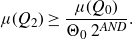
 $\Theta(Q_0)\ge M$
. Set
Footnote
2
$\Theta(Q_0)\ge M$
. Set
Footnote
2 $N = \left\lfloor A^{-2} \log\!(\Theta(Q_0)) \right\rfloor$
. Then, the family of high density cubes
$N = \left\lfloor A^{-2} \log\!(\Theta(Q_0)) \right\rfloor$
. Then, the family of high density cubes
satisfies
 \begin{equation} \sum_{Q\in{\mathsf{HD}}(Q_0)}\mu(Q) \ge (1-\Theta(Q_0)^{-s})\mu(Q_0). \end{equation}
Moreover, we have
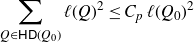 \begin{equation} \sum_{Q\in{\mathsf{HD}}(Q_0)}\ell(Q)^2\le C_p\, \ell(Q_0)^2 \end{equation}
for some dimensional constant $C_p$
(“p” stands for “packing”).
$C_p$
(“p” stands for “packing”).
The rest of this section is dedicated to proving the lemma above. For brevity of notation, we set $\Theta_0=\Theta(Q_0)$
. Observe that the integer N was chosen in such a way that
$\Theta_0=\Theta(Q_0)$
. Observe that the integer N was chosen in such a way that
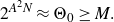 \begin{equation} 2^{A^2N}\approx \Theta_0\ge M. \end{equation}
In particular, we have $N\ge N_0$
for some very big
$N\ge N_0$
for some very big $N_0$
depending on M and A.
$N_0$
depending on M and A.
We split the proof of Lemma 3·1 into several steps.
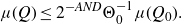
First, note that by the pigeonhole principle and (2·8), we can find a cube $Q_1 \in \mathcal{D}$
with sidelength
$Q_1 \in \mathcal{D}$
with sidelength $\ell(Q_1) = 2^{-AN} \ell(Q_0)$
,
$\ell(Q_1) = 2^{-AN} \ell(Q_0)$
, $Q_1 \subset Q_0$
, and such that
$Q_1 \subset Q_0$
, and such that
 \begin{align} \mu(Q_1) \gtrsim \frac{\mu(Q_0)}{2^{AND}}. \end{align}
Without loss of generality, by applying the appropriate translation, we can assume that $Q_1$
is centred at the origin, i.e.
$Q_1$
is centred at the origin, i.e. $p_{Q_1}=0$
. Set
$p_{Q_1}=0$
. Set
 \begin{align*} T\;:\!=\;\left\{ (z,t) \in Q_0 \, |\, |z| \leq 2^{-N} \ell(Q_0) \right\} \end{align*}
and for any $\kappa>0$
set
$\kappa>0$
set
 \begin{equation*} { T_{\kappa}}\;:\!=\;\left\{ (z,t) \in Q_0 \, |\, |z| \leq \kappa\, 2^{-N} \ell(Q_0) \right\}. \end{equation*}
Observe that $Q_1\subset T.$
In a sense, T can be seen as a tube with vertical axis passing through
$Q_1\subset T.$
In a sense, T can be seen as a tube with vertical axis passing through $p_{Q_1}=0$
. Note also that for any cube
$p_{Q_1}=0$
. Note also that for any cube $Q\subset Q_0 \setminus T$
we have
$Q\subset Q_0 \setminus T$
we have $\text{dist}(Q,Q_1)\gtrsim 2^{-N}\ell(Q_0).$
We start by proving a few preliminary results.
Lemma 3·2.
There are at most $C(\kappa)\, 2^{2N}$
cubes of sidelength
$C(\kappa)\, 2^{2N}$
cubes of sidelength $2^{-N}\ell(Q_0)$
contained in
$2^{-N}\ell(Q_0)$
contained in $T_\kappa$
.
$T_\kappa$
.
Proof. Observe that since $0\in Q_0$
, and by (2·7)
$0\in Q_0$
, and by (2·7) $Q_0\subset B(p_{Q_0},\Lambda\ell(Q_0))$
, we have
$Q_0\subset B(p_{Q_0},\Lambda\ell(Q_0))$
, we have $Q_0\subset B(0,2\Lambda\ell(Q_0)).$
Hence,
$Q_0\subset B(0,2\Lambda\ell(Q_0)).$
Hence,
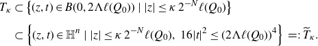 \begin{align*} T_{\kappa} &\subset \left\{ (z,t)\in B(0,2\Lambda\ell(Q_0))\ |\ |z|\le \kappa\, 2^{-N} \ell(Q_0) \right\}\\[5pt] &\subset \left\{ (z,t)\in {\mathbb{H}}^n\ |\ |z|\le \kappa\, 2^{-N} \ell(Q_0),\ 16|t|^2\le (2\Lambda \ell(Q_0))^4 \right\}\;=\!:\; \widetilde{T}_{\kappa}. \end{align*}
By (2·3),
 \begin{equation*} \mathcal{H}^{D}(\widetilde{T}_{\kappa}) = C\mathcal{L}^{2n+1}(\widetilde{T}_{\kappa}) \approx (\kappa 2^{-N} \ell(Q_0))^{2n}(2\Lambda \ell(Q_0))^2 \approx_{\kappa} 2^{-2nN}\ell(Q_0)^{D}. \end{equation*}
It follows that $\mathcal{H}^{D}(T_{\kappa})\lesssim_{\kappa}2^{-2nN}\ell(Q_0)^{D}.$
On the other hand, recall that for any cube Q with sidelength
$\mathcal{H}^{D}(T_{\kappa})\lesssim_{\kappa}2^{-2nN}\ell(Q_0)^{D}.$
On the other hand, recall that for any cube Q with sidelength $\ell(Q)=2^{-N}\ell(Q_0)$
we have
$\ell(Q)=2^{-N}\ell(Q_0)$
we have $\mathcal{H}^{D}(Q)\approx 2^{-ND}\ell(Q_0)^{D}$
. Since all such cubes are pairwise disjoint, we get
$\mathcal{H}^{D}(Q)\approx 2^{-ND}\ell(Q_0)^{D}$
. Since all such cubes are pairwise disjoint, we get
 \begin{equation*} \#\left\{Q\in\mathcal{D}\ |\ \ell(Q)=2^{-N}\ell(Q_0),\ Q\subset T_{\kappa} \right\} \lesssim \frac{\mathcal{H}^{D}(T_{\kappa})}{2^{-ND}\ell(Q_0)^{D}}\lesssim_{\kappa} \frac{2^{-2nN}\ell(Q_0)^{D}}{2^{-N(2n+2)}\ell(Q_0)^{D}}=2^{2N}. \end{equation*}
Lemma 3·3.
Let $Q\in\mathcal{D}$
satisfy
$Q\in\mathcal{D}$
satisfy $Q \subset Q_0 \setminus T$
and
$Q \subset Q_0 \setminus T$
and $\ell(Q) = \ell(Q_1)=2^{-AN}\ell(Q_0)$
. Then
$\ell(Q) = \ell(Q_1)=2^{-AN}\ell(Q_0)$
. Then
 \begin{equation} \mu(Q) \le \frac{\mu(Q_0)}{\Theta_0 \, 2^{AND}}. \end{equation}
Proof. We argue by contradiction. To this end, let us assume that there exists a cube $Q_2 \subset Q_0 \setminus T$
with
$Q_2 \subset Q_0 \setminus T$
with $\ell(Q_2)=2^{-AN}\ell(Q_0)$
such that (3·5) does not hold - that is
$\ell(Q_2)=2^{-AN}\ell(Q_0)$
such that (3·5) does not hold - that is
 \begin{equation} \mu(Q_2) \geq \frac{\mu(Q_0)}{\Theta_0 \,2^{AND}}. \end{equation}
Let $0< \delta < \text{dist}(Q_1, Q_2)$
, let
$0< \delta < \text{dist}(Q_1, Q_2)$
, let $p\in Q_2$
be arbitrary, and consider
$p\in Q_2$
be arbitrary, and consider
 \begin{equation*} R_{\mu,\delta}(\unicode{x1d7d9}_{Q_1})(p) = \int_{Q_1} K(q^{-1} \cdot p) \, d\mu(q). \end{equation*}
By triangle inequality,
 \begin{equation} |R_{\mu,\delta}(\unicode{x1d7d9}_{Q_1})(p)| \geq \left| \int_{Q_1} K(p) \, d\mu(q) \right| - \left| \int_{Q_1} K(q^{-1}\cdot p) - K(p) \, d\mu(q) \right|. \end{equation}
We estimate the first term as follows. Note that, since $p \in Q_2$
and
$p \in Q_2$
and $Q_2$
lies outside T, then, writing
$Q_2$
lies outside T, then, writing $p=(z, t)$
and using (2·4), we have
$p=(z, t)$
and using (2·4), we have
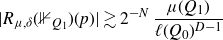
 \begin{align*} |K(p)|^2 \approx \frac{|z|^2}{(|z|^4 + 16t^2)^{n+1}} \gtrsim \frac{|z|^2}{\ell(Q_0)^{4(n+1)}} \geq 2^{-2N}\ell(Q_0)^{-4n-2} = 2^{-2N}\ell(Q_0)^{-2D+2}. \end{align*}
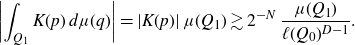
And thus we also have
 \begin{equation} \left| \int_{Q_1} K(p)\, d\mu(q) \right| = \left| K(p) \right|\mu(Q_1) \gtrsim 2^{-N} \, \frac{\mu(Q_1)}{\ell(Q_0)^{D-1}}. \end{equation}
For the second term in (3·7) we use the continuity of the kernel K (2·6) and the fact that $d(p,q) \approx \|p\|_{{\mathbb{H}}}\ge 2^{-N}\ell(Q_0)$
(because
$d(p,q) \approx \|p\|_{{\mathbb{H}}}\ge 2^{-N}\ell(Q_0)$
(because $p\in Q_2\subset Q_0\setminus T$
):
$p\in Q_2\subset Q_0\setminus T$
):
 \begin{align} |K(q^{-1} \cdot p) - K(p)| \lesssim \frac{\|q\|}{\min(\|p\|_{{\mathbb{H}}}, d(p,q))^{D}}\lesssim \frac{2^{-AN}\ell(Q_0)}{(2^{-N}\ell(Q_0))^{D}} = \frac{2^{-AN+DN}}{\ell(Q_0)^{D-1}}. \end{align}
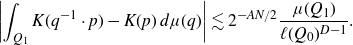
Taking $A\ge 2D$
we get
$A\ge 2D$
we get
 \begin{equation*} \left| \int_{Q_1} K(q^{-1} \cdot p) - K(p) \, d\mu(q) \right|\lesssim 2^{-AN/2}\frac{\mu(Q_1)}{\ell(Q_0)^{D-1}}. \end{equation*}
Together with (3·8) and (3·7), assuming $N_0$
bigger than some absolute constant (recall that
$N_0$
bigger than some absolute constant (recall that $N\ge N_0$
), this gives
$N\ge N_0$
), this gives
 \begin{equation*} |R_{\mu,\delta}(\unicode{x1d7d9}_{Q_1})(p)|\gtrsim 2^{-N} \, \frac{\mu(Q_1)}{\ell(Q_0)^{D-1}} \end{equation*}
for all $p\in Q_2$
.
$p\in Q_2$
.
Now, we use the estimate above and the $L^2(\mu)$
boundedness of
$L^2(\mu)$
boundedness of $R_{\mu}$
to get
$R_{\mu}$
to get
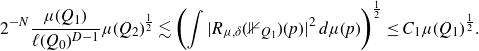 \begin{equation*} 2^{-N}\frac{\mu(Q_1)}{\ell(Q_0)^{D-1}}\mu(Q_2)^{\frac{1}{2}} \lesssim \left( \int |R_{\mu,\delta}(\unicode{x1d7d9}_{Q_1})(p)|^2 \, d\mu(p) \right)^{\frac{1}{2}} \leq C_1 \mu(Q_1)^{\frac{1}{2}}. \end{equation*}
Our assumptions on $Q_1$
(3·4) and
$Q_1$
(3·4) and $Q_2$
(3·6) yield
$Q_2$
(3·6) yield
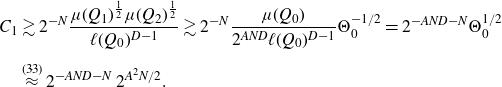 \begin{align*} C_1 & \gtrsim 2^{-N}\frac{\mu(Q_1)^{\frac{1}{2}}\mu(Q_2)^{\frac{1}{2}}}{\ell(Q_0)^{D-1}}\gtrsim 2^{-N}\frac{\mu(Q_0)}{2^{AND}\ell(Q_0)^{D-1}}\Theta_0^{-1/2} = 2^{-AND-N}\Theta_0^{1/2} \notag\\[5pt] & \overset{\scriptsize{({3\!\cdot\!3})}}{\approx} 2^{-AND-N}\, 2^{A^2 N/2}. \end{align*}
Taking $A\ge 5D$
we can bound the last term from below in the following way:
$A\ge 5D$
we can bound the last term from below in the following way:
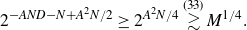 \begin{equation*} 2^{-AND-N+A^2 N/2}\ge 2^{A^2N/4}\overset{\scriptsize{({3\!\cdot\!3})}}{\gtrsim} M^{1/4}. \end{equation*}
Putting together the estimates above gives $C_1\gtrsim M^{1/4}$
, which is a contradiction for
$C_1\gtrsim M^{1/4}$
, which is a contradiction for $M=M(C_1,n)$
big enough.
$M=M(C_1,n)$
big enough.
We immediately get the following corollary.
Corollary 3·4. We have
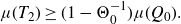 \begin{equation} \mu({T_2})\ge (1-\Theta_0^{-1})\mu(Q_0). \end{equation}
Proof. Observe that if $Q\in\mathcal{D}$
satisfies
$Q\in\mathcal{D}$
satisfies $\ell(Q) = \ell(Q_1) = 2^{-AN}\ell(Q_0)$
and
$\ell(Q) = \ell(Q_1) = 2^{-AN}\ell(Q_0)$
and $Q\not\subset T_2$
, then we have
$Q\not\subset T_2$
, then we have $Q\cap T=\varnothing$
(assuming A large enough with respect to
$Q\cap T=\varnothing$
(assuming A large enough with respect to $\Lambda$
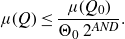
). It follows that Q satisfies the assumptions of Lemma 3·3, and so
$\Lambda$
). It follows that Q satisfies the assumptions of Lemma 3·3, and so
 \begin{equation*} \mu(Q)\le2^{-AND}\Theta_0^{-1}\mu(Q_0). \end{equation*}
Summing over all such Q and using (2·8) yields
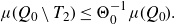 \begin{equation*} \mu(Q_0\setminus T_2) \le \Theta_0^{-1}\mu(Q_0). \end{equation*}
Recall that
 \begin{equation*} {\mathsf{HD}}(Q_0) = \left\{Q\in \mathcal{D}\ |\ Q\subset Q_0,\ \ell(Q)=2^{-N}\ell(Q_0),\ \Theta(Q)\ge;2\Theta_0 \right\}, \end{equation*}
and that $\Lambda$
is the absolute constant such that
$\Lambda$
is the absolute constant such that $Q\subset B(p_Q,\Lambda\ell(Q)).$
Without loss of generality, we may assume
$Q\subset B(p_Q,\Lambda\ell(Q)).$
Without loss of generality, we may assume $\Lambda>2$
.
$\Lambda>2$
.
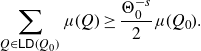
We are ready to prove the first part of Lemma 3·1, the estimate (3·1).
Lemma 3·5.
There exists $s=s(A,n)\in (0,1/2)$
such that
$s=s(A,n)\in (0,1/2)$
such that
 \begin{equation} \sum_{Q\in{\mathsf{HD}}(Q_0)}\mu(Q) \ge (1-\Theta_0^{-s})\mu(Q_0). \end{equation}
Proof. We will prove (3·11) by contradiction. Suppose that
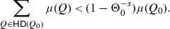 \begin{equation} \sum_{Q\in{\mathsf{HD}}(Q_0)}\mu(Q) < (1-\Theta_0^{-s})\mu(Q_0). \end{equation}
Set
 \begin{equation*} {\mathsf{LD}}(Q_0) = \left\{Q\in\mathcal{D}\ |\ Q\subset T_{2\Lambda},\ \ell(Q)=2^{-N}\ell(Q_0),\ \Theta(Q)\le 2\Theta_0 \right\}. \end{equation*}
It is easy to see that the cubes from ${\mathsf{HD}}(Q_0)\cup {\mathsf{LD}}(Q_0)$
cover
${\mathsf{HD}}(Q_0)\cup {\mathsf{LD}}(Q_0)$
cover $T_{2}$
. If we assume
$T_{2}$
. If we assume $\Theta_0\ge M>100$
, and
$\Theta_0\ge M>100$
, and $s<1/2$
, then
$s<1/2$
, then $\Theta_0^{-s}/2\ge \Theta_0^{-1}$
, and so by (3·10) and (3·12) we get
$\Theta_0^{-s}/2\ge \Theta_0^{-1}$
, and so by (3·10) and (3·12) we get
 \begin{equation} \sum_{Q\in{\mathsf{LD}}(Q_0)}\mu(Q) \ge \frac{\Theta_0^{-s}}{2}\mu(Q_0). \end{equation}
On the other hand, recall from Lemma 3·2 that there are at most $C2^{2N}$
cubes of sidelength
$C2^{2N}$
cubes of sidelength $2^{-N}\ell(Q_0)$
contained in
$2^{-N}\ell(Q_0)$
contained in $T_{2\Lambda}$
, where
$T_{2\Lambda}$
, where $C=C(\Lambda,n)$
. Moreover, for any
$C=C(\Lambda,n)$
. Moreover, for any $Q\in {\mathsf{LD}}(Q_0)$
we have
$Q\in {\mathsf{LD}}(Q_0)$
we have
 \begin{equation*} \mu(Q)\le 2 \Theta_0 \ell(Q)^{D-1}= 2\, \mu(Q_0)\frac{\ell(Q)^{D-1}}{\ell(Q_0)^{D-1}} =2^{-N(D-1)+1}\mu(Q_0). \end{equation*}
In consequence,
 \begin{equation*} \sum_{Q\in{\mathsf{LD}}(Q_0)}\mu(Q) \le C 2^{2N} 2^{-N(D-1)+1}\mu(Q_0). \end{equation*}
This contradicts (3·13) because
 \begin{equation*} C\, 2^{-ND+3N+1} = 2\, C\, (2^{-A^2N})^{(-D+3)A^{-2}} \overset{\scriptsize{({3\!\cdot\!3})}}{\le}\widetilde{C}(n)\Theta_0^{(-D+3)A^{-2}}\le \frac{\Theta_0^{-s}}{2}, \end{equation*}
choosing $s=s(A,n)$
small enough.
$s=s(A,n)$
small enough.
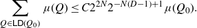
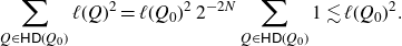
We move on to the second part of Lemma 3·1, i.e. the packing estimate (3·2).
Lemma 3·6. We have
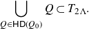 \begin{equation} \bigcup_{Q\in{\mathsf{HD}}(Q_0)}Q\subset T_{2\Lambda}. \end{equation}
In consequence,
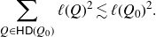 \begin{equation} \sum_{Q\in{\mathsf{HD}}(Q_0)}\ell(Q)^2\lesssim \ell(Q_0)^2. \end{equation}
Proof. We will prove that for $Q\in{\mathsf{HD}}(Q_0)$
we have
$Q\in{\mathsf{HD}}(Q_0)$
we have $Q\cap T_2\neq\varnothing.$
Then, since
$Q\cap T_2\neq\varnothing.$
Then, since $\ell(Q)=2^{-N}\ell(Q_0)$
, it follows easily from (2·7) that indeed
$\ell(Q)=2^{-N}\ell(Q_0)$
, it follows easily from (2·7) that indeed $Q\subset T_{\Lambda+2}(Q_0)\subset T_{2\Lambda}(Q_0)$
.
$Q\subset T_{\Lambda+2}(Q_0)\subset T_{2\Lambda}(Q_0)$
.
We argue by contradiction. Suppose that $Q\in {\mathsf{HD}}(Q_0)$
and
$Q\in {\mathsf{HD}}(Q_0)$
and $Q\cap T_2=\varnothing$
. Consider the cubes
$Q\cap T_2=\varnothing$
. Consider the cubes $\{P_i\}_{i\in I}$
with
$\{P_i\}_{i\in I}$
with $\ell(P_i)=2^{-AN}\ell(Q_0) = 2^{-(A-1)N}\ell(Q)$
and
$\ell(P_i)=2^{-AN}\ell(Q_0) = 2^{-(A-1)N}\ell(Q)$
and $P_i\subset Q$
. Then,
$P_i\subset Q$
. Then, $Q=\bigcup_i P_i,$
for all
$Q=\bigcup_i P_i,$
for all $i\in I$
we have
$i\in I$
we have $P_i\cap T_2=\varnothing,$
and
$P_i\cap T_2=\varnothing,$
and $\# I\approx 2^{(A-1)ND}$
by (2·8).
$\# I\approx 2^{(A-1)ND}$
by (2·8).
We use Lemma 3·3 to conclude that for all $i\in I$
 \begin{equation*} \mu(P_i) \le \frac{\mu(Q_0)}{\Theta_0 \, 2^{AND}}. \end{equation*}
Summing over $i\in I$
yields
$i\in I$
yields
 \begin{equation*} \mu(Q) = \sum_{i\in I}\mu(P_i)\le \# I\cdot \frac{\mu(Q_0)}{\Theta_0 \, 2^{AND}} \approx 2^{(A-1)ND} \frac{\mu(Q_0)}{\Theta_0 \, 2^{AND}} = \frac{\mu(Q_0)}{\Theta_0 \, 2^{ND}}, \end{equation*}
so that
 \begin{equation*} \Theta(Q) = \frac{\mu(Q)}{(2^{-N}\ell(Q_0))^{D-1}} \lesssim \frac{\mu(Q_0)}{\Theta_0 \, 2^{ND}}\cdot \frac{1}{2^{-N(D-1)}\ell(Q_0)^{D-1}} = \frac{\Theta_0}{\Theta_0 \, 2^{N}}=2^{-N}\le 1. \end{equation*}
But this contradicts the assumption $Q\in {\mathsf{HD}}(Q_0)$
:
$Q\in {\mathsf{HD}}(Q_0)$
:
 \begin{equation*} \Theta(Q)\ge 2\Theta_0\ge 2M>1, \end{equation*}
and so the proof of (3·14) is finished.
Concerning (3·15), note that by (3·14) and Lemma 3·2 we have
 \begin{equation} \# {\mathsf{HD}}(Q_0) \lesssim 2^{2N}. \end{equation}
Hence,
 \begin{align*} \sum_{Q \in {\mathsf{HD}}(Q_0)} \ell(Q)^2 = \ell(Q_0)^2\, 2^{-2N} \sum_{Q \in {\mathsf{HD}}(Q_0)} 1 \lesssim \ell(Q_0)^2. \end{align*}
4. Iteration argument
To complete the proof of Theorem 1·1, we assume that the measure $\mu$
does not satisfy the polynomial growth condition (1·1). Then we will use Lemma 3·1 countably many times to construct a set Z with positive
$\mu$
does not satisfy the polynomial growth condition (1·1). Then we will use Lemma 3·1 countably many times to construct a set Z with positive $\mu$
-measure and with Hausdorff dimension at most 2.
$\mu$
-measure and with Hausdorff dimension at most 2.
Suppose that there exists a ball B(x, r) with $\mu(B(x,r)) \geq C_2 r^{2n+1}$
; if
$\mu(B(x,r)) \geq C_2 r^{2n+1}$
; if $C_2$
is big enough, we can find a cube
$C_2$
is big enough, we can find a cube $Q_0 \in \mathcal{D},\ Q\subset B(x,r)$
such that
$Q_0 \in \mathcal{D},\ Q\subset B(x,r)$
such that
 \begin{align*} \Theta(Q_0) \ge M, \end{align*}
where M is the constant from Lemma 3·1.
Let $A>1$
be as in Lemma 3·1. Following the notation of Lemma 3·1, for an arbitrary cube
$A>1$
be as in Lemma 3·1. Following the notation of Lemma 3·1, for an arbitrary cube $Q\in\mathcal{D}$
with
$Q\in\mathcal{D}$
with $\Theta(Q)\ge M$
, set
$\Theta(Q)\ge M$
, set
 \begin{equation*} N(Q) \;:\!=\; \left\lfloor A^{-2} \log\!(\Theta(Q)) \right\rfloor\end{equation*}
and
 \begin{equation*} {\mathsf{HD}}(Q)\;:\!=\;\left\{ P \in \mathcal{D} \, |\, P\subset Q,\, \ell(P) =2^{-N(Q)}\ell(Q), \, \Theta(P) > 2 \Theta(Q) \right\}.\end{equation*}
Put $Z_{0}\;:\!=\;Q_0,\ {\mathsf{HD}}_0\;:\!=\;\{Q_0\},\ {\mathsf{HD}}_1\;:\!=\;{\mathsf{HD}}(Q_0),$
and
$Z_{0}\;:\!=\;Q_0,\ {\mathsf{HD}}_0\;:\!=\;\{Q_0\},\ {\mathsf{HD}}_1\;:\!=\;{\mathsf{HD}}(Q_0),$
and $Z_1\;:\!=\;\bigcup_{Q\in{\mathsf{HD}}_1} Q$
. Proceeding inductively, for all
$Z_1\;:\!=\;\bigcup_{Q\in{\mathsf{HD}}_1} Q$
. Proceeding inductively, for all $j\ge 2$
we define
$j\ge 2$
we define
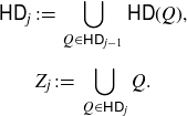 \begin{gather*} {\mathsf{HD}}_{j} \;:\!=\; \bigcup_{Q \in {\mathsf{HD}}_{j-1}} {\mathsf{HD}}(Q),\\[5pt] Z_{j} \;:\!=\; \bigcup_{Q\in{\mathsf{HD}}_j} Q.\end{gather*}
Note that for each j the cubes in ${\mathsf{HD}}_j$
form a disjoint family. Moreover,
${\mathsf{HD}}_j$
form a disjoint family. Moreover, $\{Z_j\}_{j\ge 0}$
form a decreasing sequence of sets, that is
$\{Z_j\}_{j\ge 0}$
form a decreasing sequence of sets, that is $Z_{j+1}\subset Z_j.$
Define
$Z_{j+1}\subset Z_j.$
Define
 \begin{equation*} Z \;:\!=\; \bigcap_{j \geq 0} Z_j.\end{equation*}
Claim 4·1. We have
 \begin{equation*} \mu(Z)\gtrsim_{M,s}\mu(Q_0).\end{equation*}
Proof. Observe that for $Q\in{\mathsf{HD}}_j$
we have
$Q\in{\mathsf{HD}}_j$
we have
 \begin{equation} \Theta(Q)\ge 2^{j}\Theta(Q_0)\ge 2^{j}M.\end{equation}
In particular, $\Theta(Q)\ge M$
and so we may apply Lemma 3·1 to Q. It follows that for any
$\Theta(Q)\ge M$
and so we may apply Lemma 3·1 to Q. It follows that for any $j \geq 0$
we have
$j \geq 0$
we have
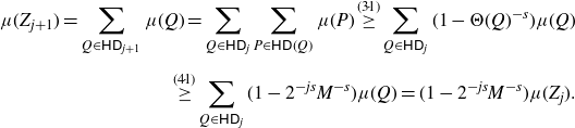 \begin{align*} \mu(Z_{j+1})=\sum_{Q \in {\mathsf{HD}}_{j+1}} \mu(Q) = \sum_{Q \in {\mathsf{HD}}_{j}} \sum_{P \in {\mathsf{HD}}(Q)} \mu(P) \stackrel{\scriptsize{({3\!\cdot\!1})}}{\geq} \sum_{Q \in {\mathsf{HD}}_{j}} (1-\Theta(Q)^{-s})\mu(Q)\\[5pt] \overset{\scriptsize{({4\!\cdot\!1})}}{\ge} \sum_{Q \in {\mathsf{HD}}_{j}} (1-2^{-js}M^{-s})\mu(Q) = (1-2^{-js}M^{-s}) \mu(Z_{j}).\end{align*}
Using this estimate $(j+1)$
times we arrive at
$(j+1)$
times we arrive at
 \begin{equation} \mu(Z_{j+1}) \geq \prod_{i=0}^{j}(1-2^{-is}M^{-s}) \mu(Q_0).\end{equation}
Since $Z_j$
form a sequence of decreasing sets, we get by the continuity of measure
$Z_j$
form a sequence of decreasing sets, we get by the continuity of measure
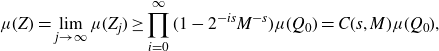 \begin{equation*} \mu(Z) = \lim_{j\to\infty} \mu(Z_j)\ge \prod_{i=0}^{\infty}(1-2^{-is}M^{-s}) \mu(Q_0) = C(s,M)\mu(Q_0),\end{equation*}
where C(s, M) is positive and finite because $\sum_{i=0}^{\infty} 2^{-is}<\infty$
.
$\sum_{i=0}^{\infty} 2^{-is}<\infty$
.
Claim 4·2. We have
 \begin{equation*} \textstyle{\text{dim}_H\!(Z)} \leq 2.\end{equation*}
Proof. Recall that $N(Q) = \left\lfloor A^{-2} \log\!(\Theta(Q)) \right\rfloor$
. It follows from (4·1) that for
$N(Q) = \left\lfloor A^{-2} \log\!(\Theta(Q)) \right\rfloor$
. It follows from (4·1) that for $Q\in{\mathsf{HD}}_j$
we have
$Q\in{\mathsf{HD}}_j$
we have $N(Q)\ge C_3jA^{-2}$
for some absolute constant
$N(Q)\ge C_3jA^{-2}$
for some absolute constant $C_3>0$
. Thus, for
$C_3>0$
. Thus, for $Q\in{\mathsf{HD}}_j$
and
$Q\in{\mathsf{HD}}_j$
and $P\in{\mathsf{HD}}(Q)$
 \begin{equation*} \ell(P)=2^{-N(Q)}\ell(Q)\le 2^{-C_3jA^{-2}}\ell(Q).\end{equation*}
Using this observation j times we get that for $P\in{\mathsf{HD}}_{j+1}$
 \begin{equation*} \ell(P)\le 2^{-C_4 j(j+1)A^{-2}}\ell(Q_0),\end{equation*}
where $C_4=C_3/2.$
Hence, the cubes from
$C_4=C_3/2.$
Hence, the cubes from ${\mathsf{HD}}_j$
form coverings of Z with decreasing diameters, well suited for estimating the Hausdorff measure of Z.
${\mathsf{HD}}_j$
form coverings of Z with decreasing diameters, well suited for estimating the Hausdorff measure of Z.
Let $0<\varepsilon<1,\ 0<\delta<1$
be small. Let
$0<\varepsilon<1,\ 0<\delta<1$
be small. Let $j\ge 0$
be so big that for
$j\ge 0$
be so big that for $Q\in{\mathsf{HD}}_{j}$
we have
$Q\in{\mathsf{HD}}_{j}$
we have $diam(Q)\le\Lambda\ell(Q)\le\delta$
. Then,
$diam(Q)\le\Lambda\ell(Q)\le\delta$
. Then,
 \begin{equation} \mathcal{H}_{\delta}^{2+\epsilon}(Z) \le \Lambda^{2+\varepsilon}\sum_{Q\in{\mathsf{HD}}_j}\ell(Q)^{2+\varepsilon}\le \Lambda^{2+\varepsilon}(2^{-C_4j(j-1)A^{-2}}\ell(Q_0))^{\varepsilon}\sum_{Q\in{\mathsf{HD}}_j}\ell(Q)^{2}.\end{equation}
It follows by (3·2) that
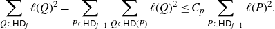 \begin{equation*} \sum_{Q\in{\mathsf{HD}}_j}\ell(Q)^{2} = \sum_{P\in{\mathsf{HD}}_{j-1}}\sum_{Q\in{\mathsf{HD}}(P)}\ell(Q)^{2}\le C_p\sum_{P\in{\mathsf{HD}}_{j-1}}\ell(P)^{2}.\end{equation*}
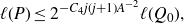
Using the estimate above j times, and putting it together with (4·3) we arrive at
 \begin{equation*} \mathcal{H}_{\delta}^{2+\epsilon}(Z) \le \Lambda^{2+\varepsilon} (C_p)^j\, \,2^{-\varepsilon C_4 j(j-1)A^{-2}}\, \ell(Q_0)^{2+\varepsilon}.\end{equation*}
The right hand side above converges to 0 as $j\to\infty$
(just note that the exponent at
$j\to\infty$
(just note that the exponent at $C_p$
is linear in j while the exponent at 2 is quadratic in j). Hence,
$C_p$
is linear in j while the exponent at 2 is quadratic in j). Hence, $\mathcal{H}_{\delta}^{2+\epsilon}(Z)=0.$
Letting
$\mathcal{H}_{\delta}^{2+\epsilon}(Z)=0.$
Letting $\delta\to 0$
we get
$\delta\to 0$
we get $\mathcal{H}^{2+\epsilon}(Z)=0.$
Since this is true for arbitrarily small
$\mathcal{H}^{2+\epsilon}(Z)=0.$
Since this is true for arbitrarily small $\epsilon>0$
, it follows that
$\epsilon>0$
, it follows that
 \begin{equation*} \textstyle{\text{dim}_H(Z)} = \inf\{t\ge 0\ :\ \mathcal{H}^t(Z)=0\} \le 2.\end{equation*}
Proof of Theorem
1·1. We have found a set $Z \subset \mathbb{H}^{n}$
of dimension smaller than or equal to 2 (Claim ) but which nevertheless has positive
$Z \subset \mathbb{H}^{n}$
of dimension smaller than or equal to 2 (Claim ) but which nevertheless has positive $\mu$
-measure (Claim ). This contradicts the assumptions of Theorem 1·1. Thus, there exists
$\mu$
-measure (Claim ). This contradicts the assumptions of Theorem 1·1. Thus, there exists $C_2=C_2(n,C_1)$
such that
$C_2=C_2(n,C_1)$
such that $\mu(B(x,r)) \leq C_2 r^{2n+1}$
for all
$\mu(B(x,r)) \leq C_2 r^{2n+1}$
for all $x\in{\mathbb{H}}^n$
and
$x\in{\mathbb{H}}^n$
and $r>0$
.
$r>0$
.
Acknowledgements
We thank Katrin Fässler and Tuomas Orponen for introducing us to the Heisenberg group and for suggesting the problem.
The bulk of this work was done while the two authors were attending the Simons Semester in Geometric Analysis at IMPAN in the Autumn 2019. We thank Tomasz Adamowicz and the staff at the institute for their hospitality.


