


1. Introduction
The study of algebraic theories and their role in modelling computing systems (Behrisch et al. Reference Behrisch, Kerkhoff and Power2012; Hyland and Power Reference Hyland and Power2007) is a recurring theme of John Power’s research, and the subject of some of his most influential contributions. In a series of articles (Garner and Power Reference Garner and Power2018; Lack and Power Reference Lack and Power2009; Power Reference Power1999, Reference Power2005), he and his coauthors developed an enriched category theoretic generalisation of Lawvere theories and explored their applications, particularly in the study of computational effects of programming languages. Whereas monads provide a powerful theory for principled and compositional definitions of denotational semantics, as pioneered by Moggi (Reference Moggi1991), algebraic theories are particularly useful (Power Reference Power2004; Power 2006 a;b) in the development of formal and principled approaches to operational semantics, as shown in a series of articles as part of a long running and productive collaboration with Gordon Plotkin (Hyland et al. Reference Hyland, Plotkin and Power2002; Reference Plotkin and PowerPlotkin and Power 2001a,b, 2002, 2003, 2004).
There have been several efforts to generalise the notion of algebraic theory in general, and that of Lawvere theory in particular. Especially after the work of Lack (Reference Lack2004), the theory of PROPs (Mac Lane Reference Mac Lane1965) – a particularly simple family of symmetric strict monoidal categories – has been advanced as a categorical tool for the study of algebraic theories, and PROPs have been applied in several parts of computer science (Baez and Erbele Reference Baez and Erbele2015; Bonchi et al. 2017 d; Bonchi et al. 2017 b; Bonchi et al. Reference Bonchi, Piedeleu, SobociŃski and Zanasi2019; Coecke and Duncan Reference Coecke and Duncan2011; Coecke and Kissinger Reference Coecke and Kissinger2017; Ghica et al. Reference Ghica, Jung and Lopez2017; Jacobs et al. Reference Jacobs, Kissinger and Zanasi2019; Sadrzadeh et al. Reference Sadrzadeh, Clark and Coecke2013; Zanasi Reference Zanasi2015). The notion of algebraic theory here is that of symmetric monoidal theory (SMT), with the essential difference being that the underlying assumption of Cartesianity is discarded. Indeed, PROPs generalise Lawvere theories, since the latter are nothing but Cartesian PROPs. The correspondence is well-behaved enough to extend to presentations of theories: indeed, it has been since long understood (Fox Reference Fox1976) that any presentation of a Lawvere theory can be seen as a presentation of a SMT (Bonchi et al. 2018 b). PROPs are more general and can be used to capture partial and relational theories (Bonchi et al. 2017 c; Corradini and Gadducci Reference Corradini and Gadducci2002; Liberti et al. Reference Liberti, Loregian, Nester and SobociŃski2021; Zanasi Reference Zanasi2016). Overall, it appears that symmetric monoidal structure is the axiomatic baseline for many pertinent examples.
One of the driving motivations for the development of rewriting theory has been the desire to implement aspects of algebraic theories. For example, the word problem for a (presentation of an) algebraic theory is decidable if one can orient the equations $l=r$
, obtaining rewriting rules
$l=r$
, obtaining rewriting rules $l\rightarrow r$
, and prove confluence and termination of the resulting rewriting system. In this way, one obtains normal forms. To decide whether two terms are judged equal by such an algebraic theory, it suffices to rewrite both until no more redexes are found, then compare the results: they are equal precisely when they rewrite to the same normal form. However, classical rewriting theory has been developed for ordinary terms, which are intimately connected with classical algebraic theories.
$l\rightarrow r$
, and prove confluence and termination of the resulting rewriting system. In this way, one obtains normal forms. To decide whether two terms are judged equal by such an algebraic theory, it suffices to rewrite both until no more redexes are found, then compare the results: they are equal precisely when they rewrite to the same normal form. However, classical rewriting theory has been developed for ordinary terms, which are intimately connected with classical algebraic theories.
The big question driving the theoretical contributions of this paper is ‘how does one implement algebraic theories captured by PROPs?’. If we take rewriting as an answer, then the rewriting has to be done up-to the axioms of symmetric strict monoidal categories.
Traditional terms enjoy a pleasantly simple structure: their syntactic decomposition may be represented as trees. Analogously, the structure of terms of symmetric monoidal categories may be represented as a particular family of string diagrams. However, there is an underlying problem: trees are combinatorial objects that are elements of a classical, inductive data type, with well-understood and efficient algorithms that are exploited for rewriting. On the other hand, string diagrams have traditionally been considered as topological entities (Joyal and Street Reference Joyal and Street1991). Our first task is therefore to understand string diagrams as combinatorial objects. In the prequel (Bonchi et al. Reference Bonchi, Gadducci, Kissinger, SobociŃski and Zanasi2022) to this paper, we showed a close connection between string diagrams over a signature $\Sigma$
and the category of discrete cospans of hypergraphs with
$\Sigma$
and the category of discrete cospans of hypergraphs with $\Sigma$
-typed edges. Nevertheless, the correspondence is not an isomorphism: for isomorphic cospans to be equated as string diagrams, they must be considered up to an underlying special Frobenius structure. While examples of such theories abound, here we consider mere symmetric monoidal structure. In Theorem 25, we characterise those cospans that arise via this correspondence, and in Proposition 27 we extend this characterisation to the multi-coloured case. The cospans of interest are those whose underlying hypergraph is acyclic and satisfies an additional technical condition that we refer to as monogamy. Checking both is algorithmically simple enough.
$\Sigma$
-typed edges. Nevertheless, the correspondence is not an isomorphism: for isomorphic cospans to be equated as string diagrams, they must be considered up to an underlying special Frobenius structure. While examples of such theories abound, here we consider mere symmetric monoidal structure. In Theorem 25, we characterise those cospans that arise via this correspondence, and in Proposition 27 we extend this characterisation to the multi-coloured case. The cospans of interest are those whose underlying hypergraph is acyclic and satisfies an additional technical condition that we refer to as monogamy. Checking both is algorithmically simple enough.
Having identified a satisfactory combinatorial representation leads us to the actual mechanism of rewriting, which is an adaptation of the DPO approach (Corradini et al. Reference Corradini, Montanari, Rossi, Ehrig, Heckel and LÖwe1997). The first modification of classical DPO is forced on us by the fact that we are rewriting cospans of hypergraphs, hence the rewriting has to be done in a way that respects the interfaces. Similar approaches have been considered previously in the literature on graph rewriting, though, the most notable example being Ehrig and KÖnig (Reference Ehrig and KÖnig2004). Second, and more seriously, the general mechanism of DPO rewriting is not sound for mere symmetric monoidal structure. The reason for this has already been highlighted in the previous paragraph: the correspondence between string diagrams and cospans of hypergraphs works when string diagrams are considered modulo the axioms of symmetric monoidal categories as well as those of the Frobenius structure. Given that we do not want to assume the presence of Frobenius, we must suitably restrict the DPO mechanism. We introduce two technical modifications: first, legal pushout complements are restricted to a variant we call boundary complements in order to preserve monogamy and acyclicity of the resulting cospan, and second, matches have to be restricted to convex matches, which have a topologically intuitive explanation. We call the resulting variant convex DPO rewriting and show that it is a sound and complete mechanism for rewriting modulo symmetric monoidal structure in Theorem 35.
To illustrate the framework, we study two examples of symmetric monoidal theories (SMTs): Frobenius semi-algebras and bialgebras. For both theories, we demonstrate straightforward proofs of termination making explicit use of the graph-theoretic structure. We furthermore show that the theory of Frobenius semi-algebras is not confluent using a surprising property of convex rewriting: namely that non-overlapping rewriting rule applications can interfere with each other. Our counter-example to confluence is adapted from an example due to Power (Reference Power1991), which was originally given in the context of pasting diagrams for 3-categories. Incidentally, Power’s example also occurred in a festschrift, in honour of Max Kelly’s 60th birthday in 1991.
This paper is based on previous conference articles (Bonchi et al. Reference Bonchi, Gadducci, Kissinger, SobociŃski and Zanasi2016; Bonchi et al. 2017 a 2018 a), and it is the second in the series, following Bonchi et al. (Reference Bonchi, Gadducci, Kissinger, SobociŃski and Zanasi2022), that collects these results in a coherent and comprehensive narrative. The formulation of our characterisation for coloured props, as well as the case studies of Frobenius semi-algebras (Section 13) and bialgebras (Section 5.2), is novel with respect to the conference papers.
Structure of the paper. Although the material in this paper is a prosecution of Bonchi et al. (Reference Bonchi, Gadducci, Kissinger, SobociŃski and Zanasi2022), we have tried to make the presentation self-contained. We give the background material in Section 2. In Section 3, we give the characterisation of string diagrams for PROPS as discrete cospans of hypergraphs that are acyclic and monogamous. In Section 7, we develop convex DPO rewriting, the mechanism that correctly implements rewriting modulo symmetric monoidal structure. Finally, in Section 13, we consider two case studies: Frobenius semi-algebras and bialgebras.
2. Background
2.1 Symmetric monoidal theories and PROPs
In this section, we recall some basic notions and fix notation. We confine ourselves to the definitions that are strictly necessary for our developments and refer the reader to the first part of this exposition (Bonchi et al. Reference Bonchi, Gadducci, Kissinger, SobociŃski and Zanasi2022) for a gentler introduction to the same notions.
A SMT is a pair $(\Sigma, \mathcal E)$
. Here,
$(\Sigma, \mathcal E)$
. Here, $\Sigma$
is a monoidal signature, consisting of operations
$\Sigma$
is a monoidal signature, consisting of operations $o \colon n \to m$
of a fixed arity n and coarity m, for
$o \colon n \to m$
of a fixed arity n and coarity m, for $n,m \in {\mathbb{N}}$
. The second element
$n,m \in {\mathbb{N}}$
. The second element $\mathcal E$
is a set of equations, namely pairs of
$\mathcal E$
is a set of equations, namely pairs of $\Sigma$
-terms
$\Sigma$
-terms $l,r \colon v \to w$
with the same arity and coarity. Recall that
$l,r \colon v \to w$
with the same arity and coarity. Recall that $\Sigma$
-terms are constructed by combining the operations in
$\Sigma$
-terms are constructed by combining the operations in $\Sigma$
, identities
$\Sigma$
, identities $\mathrm{id}_n \colon n\to n$
and symmetries
$\mathrm{id}_n \colon n\to n$
and symmetries $\sigma_{m,n} \colon m+n\to n+m$
for each
$\sigma_{m,n} \colon m+n\to n+m$
for each $m,n\in \mathbb{N}$
, by sequential (
$m,n\in \mathbb{N}$
, by sequential ( $;$
) and parallel (
$;$
) and parallel ( $\oplus$
) composition.
$\oplus$
) composition.
SMTs have a categorical rendition as PROPs (Mac Lane Reference Mac Lane1965) (monoidal product and permutation categories).
Definition 1. (PROP). A PROP is a symmetric strict monoidal category with objects the natural numbers, where the product on objects, denoted $\oplus$
, is addition. Morphisms are identity-on-objects symmetric strict monoidal functors. PROPs and their morphisms form the category
$\oplus$
, is addition. Morphisms are identity-on-objects symmetric strict monoidal functors. PROPs and their morphisms form the category ${\mathsf{PROP}}$
.
${\mathsf{PROP}}$
.
An SMT $(\Sigma, \mathcal E)$
gives raise to a PROP
$(\Sigma, \mathcal E)$
gives raise to a PROP $\mathbf{S}_{\Sigma, \mathcal E}$
by letting the arrows
$\mathbf{S}_{\Sigma, \mathcal E}$
by letting the arrows $u\to v$
of
$u\to v$
of $\mathbf{S}_{\Sigma, \mathcal E}$
be the
$\mathbf{S}_{\Sigma, \mathcal E}$
be the $\Sigma$
-terms
$\Sigma$
-terms $u\to v$
modulo the laws of symmetric monoidal categories (Figure 1) and the smallest congruence containing the equations
$u\to v$
modulo the laws of symmetric monoidal categories (Figure 1) and the smallest congruence containing the equations $t=t'$
for any
$t=t'$
for any $(t,t') \in \mathcal E$
. We are going to represent these arrows by using the graphical language of string diagrams (Selinger Reference Selinger2011). When
$(t,t') \in \mathcal E$
. We are going to represent these arrows by using the graphical language of string diagrams (Selinger Reference Selinger2011). When $\mathcal E$
is empty, we shall use notation
$\mathcal E$
is empty, we shall use notation $\mathbf{S}_{\Sigma}$
for the PROP presented by
$\mathbf{S}_{\Sigma}$
for the PROP presented by $(\Sigma, \mathcal E)$
.
$(\Sigma, \mathcal E)$
.

Figure 1. Laws of symmetric monoidal categories instantiated to a PROP ( ${\mathbb{C}}$
,
${\mathbb{C}}$
, $\oplus$
, 0), with
$\oplus$
, 0), with $m,n,p \in \mathbb{N}$
objects of
$m,n,p \in \mathbb{N}$
objects of ${\mathbb{C}}$
and s,t,u,v morphisms of
${\mathbb{C}}$
and s,t,u,v morphisms of ${\mathbb{C}}$
of the appropriate (co)arity. The laws express associativity of
${\mathbb{C}}$
of the appropriate (co)arity. The laws express associativity of $\,{;}\,$
and
$\,{;}\,$
and $\oplus$
, and how they interact with each other and with the identities. Also, they express that symmetries are natural and involutive.
$\oplus$
, and how they interact with each other and with the identities. Also, they express that symmetries are natural and involutive.
The SMT of special commutative Frobenius algebras (which we shall usually refer to simply as Frobenius algebras, for brevity) plays a special role in our developments.
Example 2 (Frobenius Algebras). Consider the SMT $(\Sigma_{\textbf{Frob}}, {\mathcal E}_{\textbf{frob}})$
, where
$(\Sigma_{\textbf{Frob}}, {\mathcal E}_{\textbf{frob}})$
, where
and ${\mathcal E}_{\textbf{frob}}$
is the set consisting of the following three equations
${\mathcal E}_{\textbf{frob}}$
is the set consisting of the following three equations
We use ${{\mathbf{Frob}}}$
to abbreviate the PROP
${{\mathbf{Frob}}}$
to abbreviate the PROP $\mathbf{S}_{(\Sigma_{{{\mathbf{Frob}}}}, {\mathcal E}_{\textbf{frob}})}$
presented by
$\mathbf{S}_{(\Sigma_{{{\mathbf{Frob}}}}, {\mathcal E}_{\textbf{frob}})}$
presented by $(\Sigma_{{{\mathbf{Frob}}}}, {\mathcal E}_{{{\mathbf{Frob}}}})$
.
$(\Sigma_{{{\mathbf{Frob}}}}, {\mathcal E}_{{{\mathbf{Frob}}}})$
.
As for regular algebraic theories, one may consider multi-coloured versions of SMTs and PROPs. What changes is the notion of signature, which is now a pair $(C, \Sigma)$
consisting of a set C of colours and a set
$(C, \Sigma)$
consisting of a set C of colours and a set $\Sigma$
of operations
$\Sigma$
of operations $o \colon w \to v$
, with
$o \colon w \to v$
, with $w, v \in C^{\star}$
words over C.
$w, v \in C^{\star}$
words over C.
Definition 3. (Coloured Prop) Given a finite set C of colours, a C-coloured PROP ${\mathbb{A}}$
is a symmetric strict monoidal category where the set of objects
${\mathbb{A}}$
is a symmetric strict monoidal category where the set of objects $C^{\star}$
is the set of the finite words over C and the monoidal product on objects is word concatenation. A morphism from a C-coloured PROP
$C^{\star}$
is the set of the finite words over C and the monoidal product on objects is word concatenation. A morphism from a C-coloured PROP ${\mathbb{A}}$
to a C’-coloured PROP
${\mathbb{A}}$
to a C’-coloured PROP ${\mathbb{A}}'$
is a symmetric strict monoidal functor
${\mathbb{A}}'$
is a symmetric strict monoidal functor $H \colon {\mathbb{A}}\rightarrow {\mathbb{A}}'$
acting on objects as a monoid homomorphism generated by a function
$H \colon {\mathbb{A}}\rightarrow {\mathbb{A}}'$
acting on objects as a monoid homomorphism generated by a function $C \to C'$
. Coloured PROPs and their morphisms form the category
$C \to C'$
. Coloured PROPs and their morphisms form the category ${\mathsf{CPROP}}$
.
${\mathsf{CPROP}}$
.
As expected, ${\mathsf{PROP}}$
is the full sub-category of
${\mathsf{PROP}}$
is the full sub-category of ${\mathsf{CPROP}}$
given by restricting to
${\mathsf{CPROP}}$
given by restricting to $\{c\}$
-coloured PROPs, for a fixed colour c.
$\{c\}$
-coloured PROPs, for a fixed colour c.
Example 4. For later use, we recall the multi-coloured analogous of Example 2, which is the theory of Frobenius algebras over a set C of colours. Its monoidal signature includes operations
(where $\varepsilon \in C^{\star}$
denotes the empty word) and equations as in Example 2 for each colour
$\varepsilon \in C^{\star}$
denotes the empty word) and equations as in Example 2 for each colour $c \in C$
. We write
$c \in C$
. We write ${{\mathbf{Frob}}}_{C}$
for the C-coloured PROP presented by this SMT.
${{\mathbf{Frob}}}_{C}$
for the C-coloured PROP presented by this SMT.
Remark 5. As observed in Bonchi et al. (2022), coproducts in ${\mathsf{CPROP}}$
work a bit differently than in
${\mathsf{CPROP}}$
work a bit differently than in ${\mathsf{PROP}}$
. Intuitively, a coproduct
${\mathsf{PROP}}$
. Intuitively, a coproduct ${\mathbb{C}} + {\mathbb{C}}'$
in
${\mathbb{C}} + {\mathbb{C}}'$
in ${\mathsf{PROP}}$
will identify the common core of the two PROPs, i.e. the set of objects
${\mathsf{PROP}}$
will identify the common core of the two PROPs, i.e. the set of objects ${\mathbb{N}}$
and the symmetrical monoidal structure on these objects. Instead, a coproduct in
${\mathbb{N}}$
and the symmetrical monoidal structure on these objects. Instead, a coproduct in ${\mathsf{CPROP}}$
will not make such identification, as the involved PROPs, say
${\mathsf{CPROP}}$
will not make such identification, as the involved PROPs, say ${\mathbb{D}}$
and
${\mathbb{D}}$
and ${\mathbb{D}}'$
, may be based on different sets of colours. However, if
${\mathbb{D}}'$
, may be based on different sets of colours. However, if ${\mathbb{D}}$
and
${\mathbb{D}}$
and ${\mathbb{D}}'$
happen to be coloured from the same set C, we may still identify their common structure. Formally, this takes the form of a pushout, which we write
${\mathbb{D}}'$
happen to be coloured from the same set C, we may still identify their common structure. Formally, this takes the form of a pushout, which we write ${\mathbb{D}} +_{\scriptscriptstyle C} {\mathbb{D}}'$
. Such pushout is obtained from the span of the inclusion morphisms
${\mathbb{D}} +_{\scriptscriptstyle C} {\mathbb{D}}'$
. Such pushout is obtained from the span of the inclusion morphisms
 $$ {\mathbb{D}}\to {{\bf{P}}_C} \to {\mathbb{D}}'$$
, where
$$ {\mathbb{D}}\to {{\bf{P}}_C} \to {\mathbb{D}}'$$
, where ${\mathbf{P}_{\scriptscriptstyle {C}}}$
is the C-coloured PROP presented by the theory with an empty signature
${\mathbf{P}_{\scriptscriptstyle {C}}}$
is the C-coloured PROP presented by the theory with an empty signature $(C, \varnothing)$
and no equations. One may think of
$(C, \varnothing)$
and no equations. One may think of ${\mathbf{P}_{\scriptscriptstyle {C}}}$
as having arrows
${\mathbf{P}_{\scriptscriptstyle {C}}}$
as having arrows $w \to v$
the permutations of w into v (thus arrows exist only when the word v is an anagram of the word w).
$w \to v$
the permutations of w into v (thus arrows exist only when the word v is an anagram of the word w).
2.2 Syntactic rewriting for PROPs
Definition 6. A rewriting rule in a PROP ${\mathbb{A}}$
consists of a pair of arrows
${\mathbb{A}}$
consists of a pair of arrows $l, r \colon i \to j$
in
$l, r \colon i \to j$
in ${\mathbb{A}}$
with the same arities and coarities, which we write as
${\mathbb{A}}$
with the same arities and coarities, which we write as ${\left\langle l,r \right\rangle}$
. Given
${\left\langle l,r \right\rangle}$
. Given $a,b \colon m \to n$
in
$a,b \colon m \to n$
in ${\mathbb{A}}$
, a rewrites into b via
${\mathbb{A}}$
, a rewrites into b via ${\mathcal{R}}$
, written
${\mathcal{R}}$
, written $a \Rightarrow_{\scriptscriptstyle {{\left\langle l,r \right\rangle}}} b$
, if they are decomposable as follows
$a \Rightarrow_{\scriptscriptstyle {{\left\langle l,r \right\rangle}}} b$
, if they are decomposable as follows
In this situation, we say that a contains a redex for ${\left\langle l,r \right\rangle}$
. A rewriting system
${\left\langle l,r \right\rangle}$
. A rewriting system ${\mathcal{R}}$
is a set of rewriting rules, where we write
${\mathcal{R}}$
is a set of rewriting rules, where we write $a \Rightarrow_{\scriptscriptstyle {{\mathcal{R}}}} b$
to mean there exists
$a \Rightarrow_{\scriptscriptstyle {{\mathcal{R}}}} b$
to mean there exists ${\left\langle l,r \right\rangle} \in {\mathcal{R}}$
such that
${\left\langle l,r \right\rangle} \in {\mathcal{R}}$
such that $a \Rightarrow_{\scriptscriptstyle {{\left\langle l,r \right\rangle}}} b$
.
$a \Rightarrow_{\scriptscriptstyle {{\left\langle l,r \right\rangle}}} b$
.
The equations $\mathcal{E}$
associated with an SMT
$\mathcal{E}$
associated with an SMT $(\Sigma,\mathcal{E})$
can be oriented as rewriting rules. They give rise to a rewriting system, in the PROP
$(\Sigma,\mathcal{E})$
can be oriented as rewriting rules. They give rise to a rewriting system, in the PROP $\mathbf{S}_{\Sigma}$
presented by
$\mathbf{S}_{\Sigma}$
presented by $(\Sigma,\varnothing)$
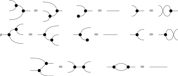
. Note that the decompositions (1) are equalities modulo the laws of Symmetric Monoidal Category (SMCs) (Figure 1). Thus, rewriting in a PROP always happens modulo these laws.
$(\Sigma,\varnothing)$
. Note that the decompositions (1) are equalities modulo the laws of Symmetric Monoidal Category (SMCs) (Figure 1). Thus, rewriting in a PROP always happens modulo these laws.
Notation 7. Note that we write generic pairs and tuples using parentheses and reserve the notation ${\left\langle l,r \right\rangle}$
specifically for the case when the pair (l,r) forms a rewriting rule.
${\left\langle l,r \right\rangle}$
specifically for the case when the pair (l,r) forms a rewriting rule.
2.3 Hypergraphs with interfaces
String diagrams in PROPs are interpreted as hypergraphs with interfaces, which we recall below.
Definition 8. (Hypergraphs). A hypergraph G consists of a set $G_\star$
of nodes and, for each
$G_\star$
of nodes and, for each $k,l \in {\mathbb{N}}$
, a (possibly empty) set of hyperedges
$k,l \in {\mathbb{N}}$
, a (possibly empty) set of hyperedges $G_{k,l}$
with k (ordered) sources and l (ordered) targets of elements in
$G_{k,l}$
with k (ordered) sources and l (ordered) targets of elements in $G_\star$
, while a hypergraph morphisms
$G_\star$
, while a hypergraph morphisms $f: G \rightarrow H$
is a family of functions
$f: G \rightarrow H$
is a family of functions $\{f_\star, f_n \mid n \in {\mathbb{N}}\}$
satisfying the expected constraints.
$\{f_\star, f_n \mid n \in {\mathbb{N}}\}$
satisfying the expected constraints.
We denote by $\mathbf{Hyp}$
the category of (finite) hypergraphs and hypergraph homomorphisms.
$\mathbf{Hyp}$
the category of (finite) hypergraphs and hypergraph homomorphisms.
Alternatively, and the characterisation will become useful later on, Hyp is the functor category ${\mathbb F}^{\mathbf{I}}$
, where
${\mathbb F}^{\mathbf{I}}$
, where ${\mathbf{I}}$
has as objects pairs of natural numbers
${\mathbf{I}}$
has as objects pairs of natural numbers $(k,l) \in {\mathbb{N}} \times {\mathbb{N}}$
together with one extra object
$(k,l) \in {\mathbb{N}} \times {\mathbb{N}}$
together with one extra object $\star$
, and, for each
$\star$
, and, for each $k,l\in{\mathbb{N}}$
, there are
$k,l\in{\mathbb{N}}$
, there are $k+l$
arrows from (k,l) to
$k+l$
arrows from (k,l) to $\star$
.odes will be drawn as dots and a (k,l) hyperedge h will be drawn as a rounded box, whose connections on the left represent the list
$\star$
.odes will be drawn as dots and a (k,l) hyperedge h will be drawn as a rounded box, whose connections on the left represent the list $[s_1(h), \ldots, s_k(h)]$
, ordered from top to bottom, and whose connections on the right represent the list
$[s_1(h), \ldots, s_k(h)]$
, ordered from top to bottom, and whose connections on the right represent the list $[t_1(h), \ldots, t_l(h)]$
.
$[t_1(h), \ldots, t_l(h)]$
.
We now introduce hypergraphs with hyperedges typed in a monoidal signature $\Sigma$
. First, define
$\Sigma$
. First, define $G_{\Sigma}$
as the hypergraph with just one node and for each
$G_{\Sigma}$
as the hypergraph with just one node and for each $k,l \in {\mathbb{N}}$
the set of
$k,l \in {\mathbb{N}}$
the set of $\Sigma$
-operations of arity k and coarity l as set of hyperedges with k sources and l targets. The category
$\Sigma$
-operations of arity k and coarity l as set of hyperedges with k sources and l targets. The category $\mathbf{Hyp}_{\Sigma}$
of
$\mathbf{Hyp}_{\Sigma}$
of $\Sigma$
-labelled hypergraphs is the category whose objects consists of an hypergraph G together with a graph homomorphism
$\Sigma$
-labelled hypergraphs is the category whose objects consists of an hypergraph G together with a graph homomorphism $\lambda: G \to G_{\Sigma}$
, which intuitively labels each hyperedge with an operation in
$\lambda: G \to G_{\Sigma}$
, which intuitively labels each hyperedge with an operation in $\Sigma$
, while labelled graph homomorphisms are defined accordingly. We call such objects
$\Sigma$
, while labelled graph homomorphisms are defined accordingly. We call such objects $\Sigma$
-hypergraphs and we visualise them as hypergraphs whose hyperedges h are labelled by
$\Sigma$
-hypergraphs and we visualise them as hypergraphs whose hyperedges h are labelled by $\lambda(h)$
. Observe that this definition ensures that a
$\lambda(h)$
. Observe that this definition ensures that a $\Sigma$
-operation
$\Sigma$
-operation $o \colon n \to m$
labels a hyperedge only when it has n (resp. m) ordered input (resp. output) nodes.
$o \colon n \to m$
labels a hyperedge only when it has n (resp. m) ordered input (resp. output) nodes.
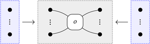
Example 9. We show our notational conventions for labelled hypergraphs with the aid of an example. The hypergraph G has nodes $\{ n_1, \ldots, n_8 \}$
, a (3,3)-hyperedge
$\{ n_1, \ldots, n_8 \}$
, a (3,3)-hyperedge $h_1$
, a (2,1)-hyperedge
$h_1$
, a (2,1)-hyperedge $h_2$
and a (1,0)-hyperedge
$h_2$
and a (1,0)-hyperedge $h_3$
, and the following source and target maps
$h_3$
, and the following source and target maps
 \begin{equation*}\begin{array}{l}s_1(h_1) := v_1 \\s_2(h_1) := v_2 \\s_3(h_1) := v_3 \\\end{array}\quad\begin{array}{l}t_1(h_1) := v_5 \\t_2(h_1) := v_6 \\t_3(h_1) := v_6\end{array}\qquad , \qquad\begin{array}{l}s_1(h_2) := v_3 \\s_2(h_2) := v_4 \\t_1(h_2) := v_8 \\\end{array}\qquad , \qquad\begin{array}{l}s_1(h_3) := v_6 \\\end{array}\end{equation*}
Also, suppose $\Sigma = \{ o_1 \colon 3 \to 3, o_2 \colon 1 \to 0, o_3 \colon 2 \to 1\}$
is a monoidal signature and
$\Sigma = \{ o_1 \colon 3 \to 3, o_2 \colon 1 \to 0, o_3 \colon 2 \to 1\}$
is a monoidal signature and $o_1$
,
$o_1$
, $o_2$
,
$o_2$
, $o_3$
label the hyperedges of G of the matching type. Then G is drawn as follows
$o_3$
label the hyperedges of G of the matching type. Then G is drawn as follows

Arrows of a PROP will receive an interpretation as labelled hyergraphs with interfaces. The notion of interface is modelled using certain cospans in $\mathbf{Hyp}_{\Sigma}$
.
$\mathbf{Hyp}_{\Sigma}$
.
Definition 10. (Hypergraphs with Interfaces). A cospan from G to G’ in $\mathbf{Hyp}_{\Sigma}$
is a pair of arrows
$\mathbf{Hyp}_{\Sigma}$
is a pair of arrows $G \xrightarrow{f} G'' \xleftarrow{g} G'$
in
$G \xrightarrow{f} G'' \xleftarrow{g} G'$
in $\mathbf{Hyp}_{\Sigma}$
, where G” is called the carrier of the cospan and G, G’ are the interfaces of G”. Two cospans
$\mathbf{Hyp}_{\Sigma}$
, where G” is called the carrier of the cospan and G, G’ are the interfaces of G”. Two cospans $G \xrightarrow{f1} G_1 \xleftarrow{g1} G'$
and
$G \xrightarrow{f1} G_1 \xleftarrow{g1} G'$
and $G \xrightarrow{f2} G_2 \xleftarrow{g2} G'$
are isomorphic when there is an isomorphism
$G \xrightarrow{f2} G_2 \xleftarrow{g2} G'$
are isomorphic when there is an isomorphism $\alpha \colon G_1 \to G_2$
in
$\alpha \colon G_1 \to G_2$
in $\mathbf{Hyp}_{\Sigma}$
making the following diagram commute
$\mathbf{Hyp}_{\Sigma}$
making the following diagram commute
We define $\mathsf{Csp}({\mathbf{Hyp}_{\Sigma}})$
as the category with the same objects as
$\mathsf{Csp}({\mathbf{Hyp}_{\Sigma}})$
as the category with the same objects as $\mathbf{Hyp}_{\Sigma}$
and arrows
$\mathbf{Hyp}_{\Sigma}$
and arrows $G \to G'$
the cospans from G to G’, up-to cospan isomorphism. Composition of
$G \to G'$
the cospans from G to G’, up-to cospan isomorphism. Composition of $G\to H \xleftarrow{f} G'$
and
$G\to H \xleftarrow{f} G'$
and $G'\xrightarrow{g} H' \leftarrow G''$
is
$G'\xrightarrow{g} H' \leftarrow G''$
is $G\to H+_{f,g}H' \leftarrow G''$
, obtained by taking the pushout of f and g.
Footnote 1
$G\to H+_{f,g}H' \leftarrow G''$
, obtained by taking the pushout of f and g.
Footnote 1
We define $\mathsf{Csp}_{D}({\mathbf{Hyp}_{\Sigma}})$
as the full subcategory of the category of cospans in
$\mathsf{Csp}_{D}({\mathbf{Hyp}_{\Sigma}})$
as the full subcategory of the category of cospans in $\mathsf{Csp}({\mathbf{Hyp}_{\Sigma}})$
with objects the discrete hypergraphs (i.e. hypergraphs with empty set of hyperedges).
$\mathsf{Csp}({\mathbf{Hyp}_{\Sigma}})$
with objects the discrete hypergraphs (i.e. hypergraphs with empty set of hyperedges).
Notation in Definition 10 follows the one introduced in Bonchi et al. (Reference Bonchi, Gadducci, Kissinger, SobociŃski and Zanasi2022), where $\mathsf{Csp}_{D}({\mathbf{Hyp}_{\Sigma}})$
is presented as an instance of a more general construction
$\mathsf{Csp}_{D}({\mathbf{Hyp}_{\Sigma}})$
is presented as an instance of a more general construction $\mathsf{Csp}_{H}({{\mathbb{C}}})$
, for a given functor H and a category
$\mathsf{Csp}_{H}({{\mathbb{C}}})$
, for a given functor H and a category ${\mathbb{C}}$
. Without going in full details, in the case of
${\mathbb{C}}$
. Without going in full details, in the case of $\mathsf{Csp}_{D}({\mathbf{Hyp}_{\Sigma}})$
, the subscript D is a functor with the role of selecting those cospans whose source and target (the interfaces) are discrete hypergraphs. This means that the objects of
$\mathsf{Csp}_{D}({\mathbf{Hyp}_{\Sigma}})$
, the subscript D is a functor with the role of selecting those cospans whose source and target (the interfaces) are discrete hypergraphs. This means that the objects of $\mathsf{Csp}_{D}({\mathbf{Hyp}_{\Sigma}})$
are natural numbers, and it is in fact a PROP.
$\mathsf{Csp}_{D}({\mathbf{Hyp}_{\Sigma}})$
are natural numbers, and it is in fact a PROP.
As with PROPs, we shall also consider the multi-coloured case of hypergraphs with interfaces. Given a set C of colours, a (multi-coloured) signature $(C, \Sigma)$
can be encoded as an hypergraph
$(C, \Sigma)$
can be encoded as an hypergraph $G_{C,\Sigma}$
: the set of nodes is C and each operation
$G_{C,\Sigma}$
: the set of nodes is C and each operation $o \colon u \to v$
yields an hyperedge, with ordered input nodes forming the word
$o \colon u \to v$
yields an hyperedge, with ordered input nodes forming the word $u \in C^{\star}$
and ordered output nodes forming the word
$u \in C^{\star}$
and ordered output nodes forming the word $v \in C^{\star}$
. We then define the category
$v \in C^{\star}$
. We then define the category $\mathbf{Hyp}_{C,\Sigma}$
of
$\mathbf{Hyp}_{C,\Sigma}$
of $(C, \Sigma)$
-labelled hypergraphs as the slice category
$(C, \Sigma)$
-labelled hypergraphs as the slice category $\mathbf{Hyp}_{} \downarrow G_{C,\Sigma}$
. Objects of
$\mathbf{Hyp}_{} \downarrow G_{C,\Sigma}$
. Objects of $\mathbf{Hyp}_{C,\Sigma}$
can be visualised as hypergraphs with nodes labelled in C and hyperedges labelled in
$\mathbf{Hyp}_{C,\Sigma}$
can be visualised as hypergraphs with nodes labelled in C and hyperedges labelled in $\Sigma$
, in a way that is compatible with the arity and coarity of operations in
$\Sigma$
, in a way that is compatible with the arity and coarity of operations in $\Sigma$
.
$\Sigma$
.
Analogously to the one-coloured case, we can form the category $\mathsf{Csp}({\mathbf{Hyp}_{C,\Sigma}})$
of cospans in
$\mathsf{Csp}({\mathbf{Hyp}_{C,\Sigma}})$
of cospans in $\mathbf{Hyp}_{C,\Sigma}$
. We will work in
$\mathbf{Hyp}_{C,\Sigma}$
. We will work in $\mathsf{Csp}_{D_C}({\mathbf{Hyp}_{C,\Sigma}})$
, the full subcategory of
$\mathsf{Csp}_{D_C}({\mathbf{Hyp}_{C,\Sigma}})$
, the full subcategory of $\mathsf{Csp}({\mathbf{Hyp}_{C,\Sigma}})$
with objects the discrete hypergraphs. Note that
$\mathsf{Csp}({\mathbf{Hyp}_{C,\Sigma}})$
with objects the discrete hypergraphs. Note that $\mathsf{Csp}_{{D_C}}({\mathbf{Hyp}_{C,\Sigma}})$
is a C-coloured PROP.
$\mathsf{Csp}_{{D_C}}({\mathbf{Hyp}_{C,\Sigma}})$
is a C-coloured PROP.
2.4 Double-pushout rewriting of hypergraphs
Double-pushout (DPO) rewriting (Corradini et al. Reference Corradini, Montanari, Rossi, Ehrig, Heckel and LÖwe1997) is an algebraic approach to rewriting that, originally given for the category of graphs, can be defined in categories whose pushouts obey certain well-behavedness conditions, called adhesive categories (Lack and SobociŃski Reference Lack and SobociŃski2005). Now, note that $\mathbf{Hyp}_{\Sigma}$
of Definition 8 can be abstractly characterised as
$\mathbf{Hyp}_{\Sigma}$
of Definition 8 can be abstractly characterised as $\mathbf{Hyp}_{} \downarrow G_{\Sigma}$
, i.e. the coslice of a presheaf category: this guarantees that it is adhesive (Bonchi et al. Reference Bonchi, Gadducci, Kissinger, SobociŃski and Zanasi2022), and thus we may apply DPO rewriting therein. In fact, in order to properly interpret string diagram rewriting, we will need a variation of DPO rewriting that takes into account interfaces. This variation, which we call DPO rewriting with interfaces (DPOI), has appeared in different guises in the literature, see e.g. Ehrig and KÖnig (Reference Ehrig and KÖnig2004), Gadducci (Reference Gadducci2007), Bonchi et al. (Reference Bonchi, Gadducci and KÖnig2009), Gadducci and Heckel (Reference Gadducci and Heckel1998), Sassone and SobociŃski (Reference Sassone and SobociŃski2005). DPOI provides a notion of rewriting for arrows
$\mathbf{Hyp}_{} \downarrow G_{\Sigma}$
, i.e. the coslice of a presheaf category: this guarantees that it is adhesive (Bonchi et al. Reference Bonchi, Gadducci, Kissinger, SobociŃski and Zanasi2022), and thus we may apply DPO rewriting therein. In fact, in order to properly interpret string diagram rewriting, we will need a variation of DPO rewriting that takes into account interfaces. This variation, which we call DPO rewriting with interfaces (DPOI), has appeared in different guises in the literature, see e.g. Ehrig and KÖnig (Reference Ehrig and KÖnig2004), Gadducci (Reference Gadducci2007), Bonchi et al. (Reference Bonchi, Gadducci and KÖnig2009), Gadducci and Heckel (Reference Gadducci and Heckel1998), Sassone and SobociŃski (Reference Sassone and SobociŃski2005). DPOI provides a notion of rewriting for arrows ${G \leftarrow J}$
in
${G \leftarrow J}$
in $\mathbf{Hyp}_{\Sigma}$
, which we write this way to emphasise that J acts as the interface of the hypergraph G, allowing G to be “glued” to a context. We now recall the definition of DPOI rewriting step.
$\mathbf{Hyp}_{\Sigma}$
, which we write this way to emphasise that J acts as the interface of the hypergraph G, allowing G to be “glued” to a context. We now recall the definition of DPOI rewriting step.
Definition 11. (DPOI Rewriting). Given $G \leftarrow J$
and
$G \leftarrow J$
and $H \leftarrow J$
in
$H \leftarrow J$
in $\mathbf{Hyp}_{\Sigma}$
, G rewrites into H with interface J — notation
$\mathbf{Hyp}_{\Sigma}$
, G rewrites into H with interface J — notation $(G \leftarrow J) \rightsquigarrow_{\scriptscriptstyle{\mathcal{R}}} (H \leftarrow J)$
— if there exist rule
$(G \leftarrow J) \rightsquigarrow_{\scriptscriptstyle{\mathcal{R}}} (H \leftarrow J)$
— if there exist rule $L \leftarrow K \rightarrow R$
in
$L \leftarrow K \rightarrow R$
in $\mathcal{R}$
and object C and cospan of arrows
$\mathcal{R}$
and object C and cospan of arrows $K \rightarrow C \leftarrow J$
in
$K \rightarrow C \leftarrow J$
in $\mathbf{Hyp}_{\Sigma}$
such that the diagram below commutes and its marked squares are pushouts
$\mathbf{Hyp}_{\Sigma}$
such that the diagram below commutes and its marked squares are pushouts
Typically, DPOI rewriting takes two distinct steps: first one computes from $K \rightarrow L \xrightarrow{m} G$
the object C and the arrows
$K \rightarrow L \xrightarrow{m} G$
the object C and the arrows $K \rightarrow C \rightarrow G$
(called a pushout complement), then one pushes out the span
$K \rightarrow C \rightarrow G$
(called a pushout complement), then one pushes out the span $C \leftarrow K \rightarrow R$
to produce the rewritten object H, preserving the interface J.
$C \leftarrow K \rightarrow R$
to produce the rewritten object H, preserving the interface J.
Pushout complements always exist in $\mathbf{Hyp}_{\Sigma}$
, but they are not necessarily unique. They are so if the rule is left-linear, that is, if
$\mathbf{Hyp}_{\Sigma}$
, but they are not necessarily unique. They are so if the rule is left-linear, that is, if $K \rightarrow L$
is monic. We will come back to this point in Section 7, as it plays an important role in giving a sound interpretation of string diagram rewriting as DPOI rewriting. For more details on the properties of pushout complements in
$K \rightarrow L$
is monic. We will come back to this point in Section 7, as it plays an important role in giving a sound interpretation of string diagram rewriting as DPOI rewriting. For more details on the properties of pushout complements in $\mathbf{Hyp}_{\Sigma}$
, we refer to Part I of this work Bonchi et al. (Reference Bonchi, Gadducci, Kissinger, SobociŃski and Zanasi2022, Section 4).
$\mathbf{Hyp}_{\Sigma}$
, we refer to Part I of this work Bonchi et al. (Reference Bonchi, Gadducci, Kissinger, SobociŃski and Zanasi2022, Section 4).
3. Combinatorial Characterisation of String Diagrams
Let us fix a monoidal signature $\Sigma$
. In Bonchi et al. (Reference Bonchi, Gadducci, Kissinger, SobociŃski and Zanasi2022), we gave an interpretation of the arrows of the PROP
$\Sigma$
. In Bonchi et al. (Reference Bonchi, Gadducci, Kissinger, SobociŃski and Zanasi2022), we gave an interpretation of the arrows of the PROP $\mathbf{S}_{\Sigma}$
in terms of cospans in
$\mathbf{S}_{\Sigma}$
in terms of cospans in $\mathbf{Hyp}_{\Sigma}$
. We also saw that to make this interpretation an isomorphism, one needs to augment
$\mathbf{Hyp}_{\Sigma}$
. We also saw that to make this interpretation an isomorphism, one needs to augment $\mathbf{S}_{\Sigma}$
with the structure of a Frobenius algebra. Formally, there are PROP morphisms
$\mathbf{S}_{\Sigma}$
with the structure of a Frobenius algebra. Formally, there are PROP morphisms
such that their copairing ${\langle\! \langle {\cdot} \rangle \! \rangle} \colon \mathbf{S}_{\Sigma} + {{\mathbf{Frob}}} \to \mathsf{Csp}_{{D}}({\mathbf{Hyp}_{\Sigma}})$
is an isomorphism of PROPs Bonchi et al. (Reference Bonchi, Gadducci, Kissinger, SobociŃski and Zanasi2022, Theorem 3.9). For the purpose of this paper, it is convenient to recall the definition of both morphisms: it suffices to define how they act on the generators, as for arbitrary arrows their action is given by induction on the structure of PROPs. The morphism
${\langle\! \langle {\cdot} \rangle \! \rangle} \colon \mathbf{S}_{\Sigma} + {{\mathbf{Frob}}} \to \mathsf{Csp}_{{D}}({\mathbf{Hyp}_{\Sigma}})$
is an isomorphism of PROPs Bonchi et al. (Reference Bonchi, Gadducci, Kissinger, SobociŃski and Zanasi2022, Theorem 3.9). For the purpose of this paper, it is convenient to recall the definition of both morphisms: it suffices to define how they act on the generators, as for arbitrary arrows their action is given by induction on the structure of PROPs. The morphism $[\!\![\cdot]\!\!] \colon \mathbf{S}_{\Sigma} \to \mathsf{Csp}_{D}({\mathbf{Hyp}_{\Sigma}})$
maps a generator
$[\!\![\cdot]\!\!] \colon \mathbf{S}_{\Sigma} \to \mathsf{Csp}_{D}({\mathbf{Hyp}_{\Sigma}})$
maps a generator $o \in \Sigma$
into the following cospan
$o \in \Sigma$
into the following cospan
where the inputs (outputs) of the edge labelled o are in bijective correspondence with the nodes of the discrete graph on the left (on the right, respectively).
For the generators of $ {{\mathbf{Frob}}}$
, the morphism
$ {{\mathbf{Frob}}}$
, the morphism ${[{\cdot]}}\colon {{\mathbf{Frob}}} \to \mathsf{Csp}_{D}({\mathbf{Hyp}_{\Sigma}})$
is defined as follows
${[{\cdot]}}\colon {{\mathbf{Frob}}} \to \mathsf{Csp}_{D}({\mathbf{Hyp}_{\Sigma}})$
is defined as follows

Note that ${\langle\! \langle {\cdot} \rangle \! \rangle} \colon \mathbf{S}_{\Sigma} + {{\mathbf{Frob}}} \to \mathsf{Csp}_{D}({\mathbf{Hyp}_{\Sigma}})$
is defined on the generators of
${\langle\! \langle {\cdot} \rangle \! \rangle} \colon \mathbf{S}_{\Sigma} + {{\mathbf{Frob}}} \to \mathsf{Csp}_{D}({\mathbf{Hyp}_{\Sigma}})$
is defined on the generators of $\mathbf{S}_{\Sigma} + {{\mathbf{Frob}}}$
, but it respects the laws of symmetric monoidal categories (Figure 1) and of Frobenius algebras (Example 2). Indeed, a major payoff of the combinatorial interpretation is that equivalent string diagrams are all interpreted as the same hypergraph with interfaces. We refer to Bonchi et al. (Reference Bonchi, Gadducci, Kissinger, SobociŃski and Zanasi2022) for more discussion on this aspect.
$\mathbf{S}_{\Sigma} + {{\mathbf{Frob}}}$
, but it respects the laws of symmetric monoidal categories (Figure 1) and of Frobenius algebras (Example 2). Indeed, a major payoff of the combinatorial interpretation is that equivalent string diagrams are all interpreted as the same hypergraph with interfaces. We refer to Bonchi et al. (Reference Bonchi, Gadducci, Kissinger, SobociŃski and Zanasi2022) for more discussion on this aspect.
In this paper, we plan to exploit $\mathsf{Csp}_{D}({\mathbf{Hyp}_{{\scriptscriptstyle {\Sigma}}}})$
as a combinatorial domain where to interpret rewriting in
$\mathsf{Csp}_{D}({\mathbf{Hyp}_{{\scriptscriptstyle {\Sigma}}}})$
as a combinatorial domain where to interpret rewriting in $\mathbf{S}_{\Sigma}$
. In the remainder of this section, we thus focus on
$\mathbf{S}_{\Sigma}$
. In the remainder of this section, we thus focus on $[\!\![\cdot]\!\!] \colon \mathbf{S}_{\Sigma} \to \mathsf{Csp}_{D}({\mathbf{Hyp}_{\Sigma}})$
and provide a combinatorial characterization of its image. A preliminary series of definitions introduces the relevant hypergraph notions: monogamy and acyclicity.
$[\!\![\cdot]\!\!] \colon \mathbf{S}_{\Sigma} \to \mathsf{Csp}_{D}({\mathbf{Hyp}_{\Sigma}})$
and provide a combinatorial characterization of its image. A preliminary series of definitions introduces the relevant hypergraph notions: monogamy and acyclicity.
Definition 12. (Degree of a node) The in-degree of a node v in hypergraph G is the number of pairs (h,i) where h is an hyperedge with v as its ith target. Similarly, the out-degree of v is the number of pairs (h,j) where h is an hyperedge with v as its jth source.
Definition 13. (Monogamy). Given $m \xrightarrow{f} G \xleftarrow{g} n$
in
$m \xrightarrow{f} G \xleftarrow{g} n$
in $\mathsf{Csp}_{D}({\mathbf{Hyp}_{{\scriptscriptstyle {\Sigma}}}})$
, let
$\mathsf{Csp}_{D}({\mathbf{Hyp}_{{\scriptscriptstyle {\Sigma}}}})$
, let $\mathsf{in}({G})$
be the image of f and
$\mathsf{in}({G})$
be the image of f and $\mathsf{out}({G})$
the image of g. We say that the cospan is monogamous if f and g are mono and for all nodes v of G
$\mathsf{out}({G})$
the image of g. We say that the cospan is monogamous if f and g are mono and for all nodes v of G
 \begin{align*}\textrm{the in-degree of {v} is } & \begin{cases} 0 &\mbox{if } v \in \mathsf{in}({G}) \\[3pt]1 & \mbox{otherwise.} \end{cases} \\[3pt]\textrm{the out-degree of {v} is } & \begin{cases} 0 &\mbox{if } v \in \mathsf{out}({G}) \\[3pt]1 & \mbox{otherwise} \end{cases}\end{align*}
We refer to the nodes in $\mathsf{in}({G})$
and
$\mathsf{in}({G})$
and $\mathsf{out}(G)$
as the inputs and the outputs of G and abusing notation we may say that G is monogamous. The cospan in (3) is clearly monogamous: all the nodes on the left are inputs and they have in-degree 0 and out-degree 1, while all the nodes on the right are outputs and they have in-degree 1 and out degree 0.
$\mathsf{out}(G)$
as the inputs and the outputs of G and abusing notation we may say that G is monogamous. The cospan in (3) is clearly monogamous: all the nodes on the left are inputs and they have in-degree 0 and out-degree 1, while all the nodes on the right are outputs and they have in-degree 1 and out degree 0.
Example 14. Four examples of cospans that are not monogamous are displayed below. In here and the reminder of the paper, we use numeric labels when we wish to specify how the cospan legs are defined on the nodes.

Lemma 15. Identities and symmetries in $ \mathsf{Csp}_{D}({\mathbf{Hyp}_{\Sigma}})$
are monogamous.
$ \mathsf{Csp}_{D}({\mathbf{Hyp}_{\Sigma}})$
are monogamous.
Proof. The cospans identifying identities and symmetries involve discrete graphs, so the in-degree and the out-degree of all nodes are 0. Moreover, all these nodes are both inputs and outputs.
Lemma 16. Let $m \rightarrow G \leftarrow n$
and
$m \rightarrow G \leftarrow n$
and $n \rightarrow H \leftarrow o$
be arrows in
$n \rightarrow H \leftarrow o$
be arrows in $ \mathsf{Csp}_{D}({\mathbf{Hyp}_{\Sigma}})$
. If both are monogamous cospans, then
$ \mathsf{Csp}_{D}({\mathbf{Hyp}_{\Sigma}})$
. If both are monogamous cospans, then $(m \rightarrow G \leftarrow n) \, ; \, (n \rightarrow H \leftarrow o)$
is monogamous.
$(m \rightarrow G \leftarrow n) \, ; \, (n \rightarrow H \leftarrow o)$
is monogamous.
Proof. Since pushouts along monos in $\mathbf{Hyp}_{\Sigma}$
are mono, the morphisms of the cospans resulting from the composition
$\mathbf{Hyp}_{\Sigma}$
are mono, the morphisms of the cospans resulting from the composition $(m \rightarrow G \leftarrow n) \, ; \, (n \rightarrow H \leftarrow o)$
are also mono. The condition on degrees is trivially preserved since
$(m \rightarrow G \leftarrow n) \, ; \, (n \rightarrow H \leftarrow o)$
are also mono. The condition on degrees is trivially preserved since $(m \rightarrow G \leftarrow n) \, ; \, (n \rightarrow H \leftarrow o)$
is obtained by gluing together G with H along the nodes in n. This means that each of the nodes in
$(m \rightarrow G \leftarrow n) \, ; \, (n \rightarrow H \leftarrow o)$
is obtained by gluing together G with H along the nodes in n. This means that each of the nodes in $\mathsf{out}(G)$
is identified with exactly one of the node in
$\mathsf{out}(G)$
is identified with exactly one of the node in $\mathsf{in}({H})$
.
$\mathsf{in}({H})$
. ![]()
Lemma 17. Let $m_1 \rightarrow G_1 \leftarrow n_1$
and
$m_1 \rightarrow G_1 \leftarrow n_1$
and $m_2 \rightarrow G_2 \leftarrow n_2$
be arrows in
$m_2 \rightarrow G_2 \leftarrow n_2$
be arrows in $\mathsf{Csp}_{D}({\mathbf{Hyp}_{\Sigma}})$
. If both are monogamous cospans, then
$\mathsf{Csp}_{D}({\mathbf{Hyp}_{\Sigma}})$
. If both are monogamous cospans, then $(m_1 \rightarrow G_1 \leftarrow n_1) \, {\oplus} \, (m_2 \rightarrow G_2 \leftarrow n_2)$
is monogamous.
$(m_1 \rightarrow G_1 \leftarrow n_1) \, {\oplus} \, (m_2 \rightarrow G_2 \leftarrow n_2)$
is monogamous.
Proof. By definition $(m_1 \rightarrow G_1 \leftarrow n_1) \, {\oplus} \, (m_2 \rightarrow G_2 \leftarrow n_2)$
is obtained by coproduct and therefore the degree of each node is the same as in the original graphs
$(m_1 \rightarrow G_1 \leftarrow n_1) \, {\oplus} \, (m_2 \rightarrow G_2 \leftarrow n_2)$
is obtained by coproduct and therefore the degree of each node is the same as in the original graphs $G_1$
and
$G_1$
and $G_2$
. Moreover, each node is an input iff it is an input in
$G_2$
. Moreover, each node is an input iff it is an input in $G_1$
or in
$G_1$
or in $G_2$
and it is an output iff it is an output in
$G_2$
and it is an output iff it is an output in $G_1$
or
$G_1$
or $G_2$
.
$G_2$
. ![]()
The notions of acyclicity and (directed) path between two nodes in a (directed) graph generalises to (directed) hypergraphs in the obvious way.
Definition 18. For a pair of hyperedges h,h’, we call h a predecessor of h’ and h’ a successor of h if there exists a node v in the target of h and in the source of h’.
Definition 19. (Path) For a hypergraph G and hyperedges h,h’, a path p from h to h’ is a sequence of hyperedges $[h_1, \ldots, h_n]$
such that
$[h_1, \ldots, h_n]$
such that $h_1 = h$
,
$h_1 = h$
, $h_n = h'$
, and for
$h_n = h'$
, and for $i < n$
,
$i < n$
, $h_{i+1}$
is a successor of
$h_{i+1}$
is a successor of $h_i$
. We say p starts at a subgraph H if H contains a node in the source of h, and terminates at a subgraph H’ if H’ contains a node in the target of h’.
$h_i$
. We say p starts at a subgraph H if H contains a node in the source of h, and terminates at a subgraph H’ if H’ contains a node in the target of h’.
By regarding nodes as single-node subgraphs, it clearly makes sense to talk about paths from/to nodes as well.
Definition 20. (Acyclicity) A hypergraph G is acyclic if there exists no path from a node to itself. We also call a cospan $m \rightarrow G \leftarrow n$
acyclic if the property holds for G.
$m \rightarrow G \leftarrow n$
acyclic if the property holds for G.
Like for monogamy, it is easy to see that identities and symmetries are acyclic and that the monoidal product of acyclic cospans is acyclic. Unfortunately, the composition of two acyclic cospans might be cyclic: for instance by composing the following two acyclic cospans

one obtains the cyclic cospan

This issue can be avoided by additionally requiring the cospans to be monogamous.
Proposition 21. Let $m \rightarrow G \leftarrow n$
,
$m \rightarrow G \leftarrow n$
, $n \rightarrow H \leftarrow o$
,
$n \rightarrow H \leftarrow o$
, $m_1 \rightarrow G_1 \leftarrow n_1$
and
$m_1 \rightarrow G_1 \leftarrow n_1$
and $m_2 \rightarrow G_2 \leftarrow n_2$
be monogamous acyclic cospans.
$m_2 \rightarrow G_2 \leftarrow n_2$
be monogamous acyclic cospans.
-
(1). Identities and symmetries in $\mathsf{Csp}_{D}({\mathbf{Hyp}_{\Sigma}})$
are monogamous acyclic.
$\mathsf{Csp}_{D}({\mathbf{Hyp}_{\Sigma}})$
are monogamous acyclic. -
(2).
$(m \rightarrow G \leftarrow n) \, ; \, (n \rightarrow H \leftarrow o)$
is monogamous acyclic. -
(3).
$(m_1 \rightarrow G_1 \leftarrow n_1) \, {\oplus} \, (m_2 \rightarrow G_2 \leftarrow n_2)$
is monogamous acyclic.


Proof. The first and the third points follow from what we discussed so far. The second point is the most interesting one. From Lemma 16, it follows immediately that $(m \rightarrow G \leftarrow n) \, ; \, (n \rightarrow H \leftarrow o)$
is monogamous, so we only need to show that this is acyclic. Since both
$(m \rightarrow G \leftarrow n) \, ; \, (n \rightarrow H \leftarrow o)$
is monogamous, so we only need to show that this is acyclic. Since both $m \rightarrow G \leftarrow n$
and
$m \rightarrow G \leftarrow n$
and $n \rightarrow H \leftarrow o$
are monogamous, their composition just identifies each of the nodes in
$n \rightarrow H \leftarrow o$
are monogamous, their composition just identifies each of the nodes in $\mathsf{out}(G)$
with exactly one node in
$\mathsf{out}(G)$
with exactly one node in $\mathsf{in}({H})$
. The identification of these nodes cannot create any cycle since there is no path in G starting with one of these nodes (since their out-degree in G is 0) and there is no path in H arriving in one of these nodes (since their in-degree in H is 0).
$\mathsf{in}({H})$
. The identification of these nodes cannot create any cycle since there is no path in G starting with one of these nodes (since their out-degree in G is 0) and there is no path in H arriving in one of these nodes (since their in-degree in H is 0). ![]()
The above proposition informs us that monogamous acyclic cospans form a sub-PROP of $\mathsf{Csp}_{D}({\mathbf{Hyp}_{\Sigma}})$
, which we call hereafter
$\mathsf{Csp}_{D}({\mathbf{Hyp}_{\Sigma}})$
, which we call hereafter $\mathsf{MACsp}_{{D}}({\mathbf{Hyp}_{\Sigma}})$
. The main result of this section (Theorem 25) shows that
$\mathsf{MACsp}_{{D}}({\mathbf{Hyp}_{\Sigma}})$
. The main result of this section (Theorem 25) shows that $\mathsf{MACsp}_{D}({\mathbf{Hyp}_{\Sigma}})$
is exactly the image of
$\mathsf{MACsp}_{D}({\mathbf{Hyp}_{\Sigma}})$
is exactly the image of $\mathbf{S}_{\Sigma}$
through
$\mathbf{S}_{\Sigma}$
through $[\!\![\cdot]\!\!]$
. Its proof relies on an additional definition and a decomposition lemma.
$[\!\![\cdot]\!\!]$
. Its proof relies on an additional definition and a decomposition lemma.
Definition 22. (Convex sub-hypergraph) A sub-hypergraph $H \subseteq G$
is convex if, for any nodes v, v’ in H and any path p from v to v’ in G, every hyperedge in p is also in H.
$H \subseteq G$
is convex if, for any nodes v, v’ in H and any path p from v to v’ in G, every hyperedge in p is also in H.
Example 23. Consider the following hypergraph

Below on the left and on the right are illustrated a convex and a non-convex sub-hypergraph

Lemma 24. (Decomposition) Let $m \rightarrow G \leftarrow n$
be a monogamous acyclic cospan and L a convex sub-hypergraph of G. Then there exist
$m \rightarrow G \leftarrow n$
be a monogamous acyclic cospan and L a convex sub-hypergraph of G. Then there exist $k\in{\mathbb{N}}$
and a unique cospan
$k\in{\mathbb{N}}$
and a unique cospan $i \rightarrow L \leftarrow j$
such that G factors as
$i \rightarrow L \leftarrow j$
such that G factors as

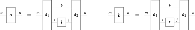
where all cospans in (4) are monogamous acyclic.
Proof. Let $C_1$
be the smallest sub-hypergraph containing the inputs of G and every hyperedge h that is not in L, but has a path to it. Let
$C_1$
be the smallest sub-hypergraph containing the inputs of G and every hyperedge h that is not in L, but has a path to it. Let $C_2$
then be the smallest sub-hypergraph containing the outputs of G such that
$C_2$
then be the smallest sub-hypergraph containing the outputs of G such that $C_1 \cup L \cup C_2 = G$
. By construction,
$C_1 \cup L \cup C_2 = G$
. By construction, $C_1$
and L share no hyperedges. Should
$C_1$
and L share no hyperedges. Should $C_2$
share a hyperedge with
$C_2$
share a hyperedge with $C_1$
or L, then a smaller
$C_1$
or L, then a smaller $C_2'$
would exist such that
$C_2'$
would exist such that $C_1 \cup L \cup C_2' = G$
, so
$C_1 \cup L \cup C_2' = G$
, so $C_2$
shares no hyperedges with either
$C_2$
shares no hyperedges with either $C_1$
or L. Hence, the three sub-hypergraphs only overlap on nodes. Now let
$C_1$
or L. Hence, the three sub-hypergraphs only overlap on nodes. Now let
 \begin{align*} i & := {C_1}_\ast \cap L_\ast \\[2pt] j & := {C_2}_\ast \cap L_\ast \\[2pt] k & := ({C_1}_\ast \cap {C_2}_\ast) \backslash L_\ast \end{align*}
where $L_\ast$
are the nodes of hypergraph L and the same for
$L_\ast$
are the nodes of hypergraph L and the same for $C_1$
and
$C_1$
and $C_2$
. Pictorially, these sub-hypergraphs are defined as follows
$C_2$
. Pictorially, these sub-hypergraphs are defined as follows

Now, define the following cospans, where arrows are all inclusions
 \begin{align*} m \rightarrow C_1 \leftarrow k + i\\[3pt] i \rightarrow L \leftarrow j\\[3pt] k + j \rightarrow C_2 \leftarrow n \end{align*}
Then (4) is computed as the colimit of the following diagram
 \begin{equation*} m \rightarrow C_1 \leftarrow k + i \rightarrow k + L \leftarrow k + j \rightarrow C_2 \leftarrow n \end{equation*}
The two spans identify precisely those nodes from G that occur in more than one sub-hypergraph, so this amounts to simply taking the union
 \begin{equation*} m \rightarrow C_1 \cup L \cup C_2 \leftarrow n \ =\ m \rightarrow G \leftarrow n \end{equation*}
Now $C_1, C_2$
and L are acyclic because G is, so it only remains to show that each of these cospans is monogamous. For
$C_1, C_2$
and L are acyclic because G is, so it only remains to show that each of these cospans is monogamous. For $C_1$
and
$C_1$
and $C_2$
it follows straightforwardly from the observation that, by construction,
$C_2$
it follows straightforwardly from the observation that, by construction, $C_1$
is closed under predecessors and
$C_1$
is closed under predecessors and $C_2$
under successors. The interesting case is L, which relies on convexity. Suppose v has no in-hyperedge in L. Then either v is an input or there exists a hyperedge with a path to v. One of these two is true precisely when
$C_2$
under successors. The interesting case is L, which relies on convexity. Suppose v has no in-hyperedge in L. Then either v is an input or there exists a hyperedge with a path to v. One of these two is true precisely when $v \in i$
. Suppose v has no out-hyperedge in L. Then, either v is an ouput or it has an out-hyperedge in
$v \in i$
. Suppose v has no out-hyperedge in L. Then, either v is an ouput or it has an out-hyperedge in $C_1$
or
$C_1$
or $C_2$
. But if it has an out-hyperedge h in
$C_2$
. But if it has an out-hyperedge h in $C_1$
, then there is a path from v to another node v’, going through h. By convexity, h must then be in L, which is a contradiction. Hence,
$C_1$
, then there is a path from v to another node v’, going through h. By convexity, h must then be in L, which is a contradiction. Hence, $v \in C_2$
, which is true if and only if
$v \in C_2$
, which is true if and only if $v \in j$
.
$v \in j$
. ![]()
Theorem 25. A cospan $n \rightarrow G \leftarrow m$
is in the image of
$n \rightarrow G \leftarrow m$
is in the image of $[\!\![\cdot]\!\!]\colon \mathbf{S}_{\Sigma} \to \mathsf{Csp}_{{D}}({\mathbf{Hyp}_{\Sigma}})$
if and only if
$[\!\![\cdot]\!\!]\colon \mathbf{S}_{\Sigma} \to \mathsf{Csp}_{{D}}({\mathbf{Hyp}_{\Sigma}})$
if and only if $n \rightarrow G \leftarrow m$
is monogamous acyclic.
$n \rightarrow G \leftarrow m$
is monogamous acyclic.
Proof. The only if direction follows by induction on the arrows of $\mathbf{S}_{\Sigma}$
: for the base case, it is immediate to check that (3) is monogamous acyclic, while the inductive cases follow from Proposition 21.
$\mathbf{S}_{\Sigma}$
: for the base case, it is immediate to check that (3) is monogamous acyclic, while the inductive cases follow from Proposition 21.
For the converse direction, we can reason by induction on the number of hyperedges in G. If G does not contain any, then monogamy and acyclicity imply that $n\rightarrow G$
and
$n\rightarrow G$
and $m\rightarrow G$
are bijections, so that
$m\rightarrow G$
are bijections, so that $n \rightarrow G \leftarrow m$
is in the image of an arrow only consisting of identities and symmetries. For the inductive step, pick any hyperedge e of G. Recall that e has a label
$n \rightarrow G \leftarrow m$
is in the image of an arrow only consisting of identities and symmetries. For the inductive step, pick any hyperedge e of G. Recall that e has a label $l(e)\in \Sigma$
and that l(e) is an arrow of
$l(e)\in \Sigma$
and that l(e) is an arrow of $\mathbf{S}_{\Sigma}$
. By monogamy and acyclicity,
$\mathbf{S}_{\Sigma}$
. By monogamy and acyclicity, $[\!\![1(e)]\!\!]$
is a convex sub-hypergraph of G. Hence, by Lemma 24,
$[\!\![1(e)]\!\!]$
is a convex sub-hypergraph of G. Hence, by Lemma 24, $n \rightarrow G \leftarrow m$
factors as (4), with L being
$n \rightarrow G \leftarrow m$
factors as (4), with L being $[\!\![1(e)]\!\!]$
. The lemma guarantees that all the above cospans are monogamous acyclic. Therefore, by the inductive hypothesis they are in the image of
$[\!\![1(e)]\!\!]$
. The lemma guarantees that all the above cospans are monogamous acyclic. Therefore, by the inductive hypothesis they are in the image of $[\!\![\cdot]\!\!]$
, and so the same holds for
$[\!\![\cdot]\!\!]$
, and so the same holds for $n \rightarrow G \leftarrow m$
.
$n \rightarrow G \leftarrow m$
. ![]()
The following result (Corollary 3.11 in Bonchi et al. Reference Bonchi, Gadducci, Kissinger, SobociŃski and Zanasi2022) proves that $[\!\![\cdot]\!\!]\colon \mathbf{S}_{\Sigma} \to \mathsf{Csp}_{D}({\mathbf{Hyp}_{\Sigma}})$
is faithful, so an immediate consequence of the above theorem is that
$[\!\![\cdot]\!\!]\colon \mathbf{S}_{\Sigma} \to \mathsf{Csp}_{D}({\mathbf{Hyp}_{\Sigma}})$
is faithful, so an immediate consequence of the above theorem is that $ \mathbf{S}_{\Sigma}$
is isomorphic to the sub-PROP of
$ \mathbf{S}_{\Sigma}$
is isomorphic to the sub-PROP of $\mathsf{Csp}_{D}({\mathbf{Hyp}_{\Sigma}})$
of monogamous acyclic cospans.
$\mathsf{Csp}_{D}({\mathbf{Hyp}_{\Sigma}})$
of monogamous acyclic cospans.
Corollary 26. $ \mathbf{S}_{\Sigma} \cong \mathsf{MACsp}_{{D}}({\mathbf{Hyp}_{\Sigma}})$
.
$ \mathbf{S}_{\Sigma} \cong \mathsf{MACsp}_{{D}}({\mathbf{Hyp}_{\Sigma}})$
.
3.1 Characterisation for coloured PROPs
At the beginning of this section, we recalled from Bonchi et al. (Reference Bonchi, Gadducci, Kissinger, SobociŃski and Zanasi2022) that $\mathsf{Csp}_{D}({\mathbf{Hyp}_{\Sigma}})$
is isomorphic to
$\mathsf{Csp}_{D}({\mathbf{Hyp}_{\Sigma}})$
is isomorphic to $\mathbf{S}_{\Sigma} + {{\mathbf{Frob}}} $
. The isomorphism extends in the obvious way to the coloured case: Proposition 3.12 in Bonchi et al. (Reference Bonchi, Gadducci, Kissinger, SobociŃski and Zanasi2022) states that
$\mathbf{S}_{\Sigma} + {{\mathbf{Frob}}} $
. The isomorphism extends in the obvious way to the coloured case: Proposition 3.12 in Bonchi et al. (Reference Bonchi, Gadducci, Kissinger, SobociŃski and Zanasi2022) states that $\mathsf{Csp}_{D_C}({\mathbf{Hyp}_{C,\Sigma}})$
is isomorphic to
$\mathsf{Csp}_{D_C}({\mathbf{Hyp}_{C,\Sigma}})$
is isomorphic to $\mathbf{S}_{C,\Sigma} +_C {{\mathbf{Frob}_{C}}}$
(where
$\mathbf{S}_{C,\Sigma} +_C {{\mathbf{Frob}_{C}}}$
(where $+_C$
and
$+_C$
and ${{\mathbf{Frob}_{C}}}$
are defined as in Example 4 and Remark 5). The same holds for Theorem 25. The definition of
${{\mathbf{Frob}_{C}}}$
are defined as in Example 4 and Remark 5). The same holds for Theorem 25. The definition of $[\!\![\cdot]\!\!]_C$
given in Bonchi et al. (Reference Bonchi, Gadducci, Kissinger, SobociŃski and Zanasi2022) is the same as the one in (3), but with the proper interpretation of colours as labels of nodes. The definition of monogamous acyclic cospans (Definitions 13 and 20) does not change: the notions of degree and path are exactly the same in coloured and non coloured hypergraphs. All the results proved above hold straightforwardly by following the same proofs. In particular, we have the following.
$[\!\![\cdot]\!\!]_C$
given in Bonchi et al. (Reference Bonchi, Gadducci, Kissinger, SobociŃski and Zanasi2022) is the same as the one in (3), but with the proper interpretation of colours as labels of nodes. The definition of monogamous acyclic cospans (Definitions 13 and 20) does not change: the notions of degree and path are exactly the same in coloured and non coloured hypergraphs. All the results proved above hold straightforwardly by following the same proofs. In particular, we have the following.
Theorem 27. A cospan $w \rightarrow G \leftarrow v$
is in the image of
$w \rightarrow G \leftarrow v$
is in the image of $[\!\![\cdot]\!\!]_C \colon \mathbf{S}_{C, \Sigma} \to \mathsf{Csp}_{{D_C}}({\mathbf{Hyp}_{C, \Sigma}})$
if and only if
$[\!\![\cdot]\!\!]_C \colon \mathbf{S}_{C, \Sigma} \to \mathsf{Csp}_{{D_C}}({\mathbf{Hyp}_{C, \Sigma}})$
if and only if $w \rightarrow G \leftarrow v$
is monogamous acyclic.
$w \rightarrow G \leftarrow v$
is monogamous acyclic.
4. A Sound and Complete Interpretation for String Diagram Rewriting
In this section, we develop a version of DPOI rewriting that is sound and complete for symmetric monoidal categories that do not come with a chosen Frobenius algebra on each object. Recall that, as shown in Bonchi et al. (Reference Bonchi, Gadducci, Kissinger, SobociŃski and Zanasi2022), DPOI rewriting for hypergraphs (Definition 11) corresponds exactly to the rewriting for a SMT $\Sigma$
, modulo Frobenius structure.
$\Sigma$
, modulo Frobenius structure.
Before formally stating this correspondence (Theorem 28 below), we recall from Bonchi et al. (Reference Bonchi, Gadducci, Kissinger, SobociŃski and Zanasi2022) the notation ${\ulcorner {d} \urcorner}$
, which refers to the ‘rewiring’ of a syntactic term d, turning all of the inputs into outputs
${\ulcorner {d} \urcorner}$
, which refers to the ‘rewiring’ of a syntactic term d, turning all of the inputs into outputs

Working with ‘rewired’ graphs is equivalent to working with the original ones, in the sense that $d \Rightarrow_{\scriptscriptstyle {{\left\langle l,r \right\rangle}}} e$
if and only if
$d \Rightarrow_{\scriptscriptstyle {{\left\langle l,r \right\rangle}}} e$
if and only if ${\ulcorner {d} \urcorner} \Rightarrow_{\scriptscriptstyle {{\left\langle {{\ulcorner {l} \urcorner}},{{\ulcorner {r} \urcorner}} \right\rangle}}} {\ulcorner {e} \urcorner}$
. However, since the rewired rules have only one boundary, they are readily interpreted as hypergraphs with interfaces. That is, if d corresponds to a cospan
${\ulcorner {d} \urcorner} \Rightarrow_{\scriptscriptstyle {{\left\langle {{\ulcorner {l} \urcorner}},{{\ulcorner {r} \urcorner}} \right\rangle}}} {\ulcorner {e} \urcorner}$
. However, since the rewired rules have only one boundary, they are readily interpreted as hypergraphs with interfaces. That is, if d corresponds to a cospan $i \rightarrow G \leftarrow j$
, then
$i \rightarrow G \leftarrow j$
, then ${\ulcorner {d} \urcorner}$
corresponds to
${\ulcorner {d} \urcorner}$
corresponds to $0 \rightarrow G \leftarrow i + j$
, or simply
$0 \rightarrow G \leftarrow i + j$
, or simply $G \leftarrow i + j$
.
$G \leftarrow i + j$
.
Similarly, a syntactic rewriting rule ${\left\langle {{\ulcorner {l} \urcorner}},{{\ulcorner {r} \urcorner}} \right\rangle}$
corresponds to a pair of hypergraphs with the same interface,
${\left\langle {{\ulcorner {l} \urcorner}},{{\ulcorner {r} \urcorner}} \right\rangle}$
corresponds to a pair of hypergraphs with the same interface, $L \leftarrow i+j$
and
$L \leftarrow i+j$
and $R \leftarrow i+j$
, i.e. a span
$R \leftarrow i+j$
, i.e. a span $L \leftarrow i + j \rightarrow R$
. Hence, we can extend the definition of
$L \leftarrow i + j \rightarrow R$
. Hence, we can extend the definition of ${\langle\! \langle {\cdot} \rangle \! \rangle} \colon \mathbf{S}_{\Sigma} + {{\mathbf{Frob}}} \to \mathsf{Csp}_{D}({\mathbf{Hyp}_{\Sigma}})$
(cf. Section 3) to rewriting rules by letting
${\langle\! \langle {\cdot} \rangle \! \rangle} \colon \mathbf{S}_{\Sigma} + {{\mathbf{Frob}}} \to \mathsf{Csp}_{D}({\mathbf{Hyp}_{\Sigma}})$
(cf. Section 3) to rewriting rules by letting ${\langle\! \langle {{\left\langle {{\ulcorner {l} \urcorner}},{{\ulcorner {r} \urcorner}} \right\rangle}} \rangle \! \rangle} := L \leftarrow i+j \rightarrow R$
. We now have all the ingredients to recall the correspondence theorem between (syntactic) rewriting modulo Frobenius relation
${\langle\! \langle {{\left\langle {{\ulcorner {l} \urcorner}},{{\ulcorner {r} \urcorner}} \right\rangle}} \rangle \! \rangle} := L \leftarrow i+j \rightarrow R$
. We now have all the ingredients to recall the correspondence theorem between (syntactic) rewriting modulo Frobenius relation $\Rightarrow$
and the DPOI rewriting relation
$\Rightarrow$
and the DPOI rewriting relation $\rightsquigarrow_{\scriptscriptstyle}$
.
$\rightsquigarrow_{\scriptscriptstyle}$
.
Theorem 28
(
Reference Bonchi, Gadducci, Kissinger, SobociŃski and Zanasi
Bonchi et al. 2022
) Let ${\left\langle l,r \right\rangle}$
be a rewriting rule on
${\left\langle l,r \right\rangle}$
be a rewriting rule on $\mathbf{S}_{\Sigma}+{{\mathbf{Frob}}}$
. Then
$\mathbf{S}_{\Sigma}+{{\mathbf{Frob}}}$
. Then
 \begin{equation*}d \Rightarrow_{\scriptscriptstyle {{\left\langle l,r \right\rangle}}} e \quad \mathrm{ iff } \quad {\langle\! \langle {{\ulcorner {d} \urcorner}} \rangle \! \rangle} \rightsquigarrow_{\scriptscriptstyle{{\langle\! \langle {{\left\langle {{\ulcorner {l} \urcorner}},{{\ulcorner {r} \urcorner}} \right\rangle}} \rangle \! \rangle}}} {\langle\! \langle {{\ulcorner {e} \urcorner}} \rangle \! \rangle}\mathrm{ .}\end{equation*}
In this section, we will see that the full DPOI relation $\rightsquigarrow_{\scriptscriptstyle}$
is not sound for rewriting in the absence of Frobenius structure. To fix this problem, we will put a restriction on which pushout complements (i.e. contexts) are allowed in a rewriting step. If a rule is not left-linear, there could be many different pushout complements for a given match, each one yielding a different result. It was shown in Bonchi et al. (Reference Bonchi, Gadducci, Kissinger, SobociŃski and Zanasi2022) that this makes perfect sense when rewriting modulo Frobenius structure. However, without this structure not all results can be interpreted in a symmetric monoidal category.
$\rightsquigarrow_{\scriptscriptstyle}$
is not sound for rewriting in the absence of Frobenius structure. To fix this problem, we will put a restriction on which pushout complements (i.e. contexts) are allowed in a rewriting step. If a rule is not left-linear, there could be many different pushout complements for a given match, each one yielding a different result. It was shown in Bonchi et al. (Reference Bonchi, Gadducci, Kissinger, SobociŃski and Zanasi2022) that this makes perfect sense when rewriting modulo Frobenius structure. However, without this structure not all results can be interpreted in a symmetric monoidal category.
Example 29. Consider $\Sigma = \{ \alpha_1 \colon 0 \to 1, \alpha_2 \colon 1\to 0, \alpha_3 \colon 1 \to 1\}$
and the PROP rewriting system
$\Sigma = \{ \alpha_1 \colon 0 \to 1, \alpha_2 \colon 1\to 0, \alpha_3 \colon 1 \to 1\}$
and the PROP rewriting system $\mathbf{S}_{\Sigma}$
. Its interpretation in
$\mathbf{S}_{\Sigma}$
. Its interpretation in $\mathsf{Csp}_{D}({\mathbf{Hyp}_{{\scriptscriptstyle {\Sigma}}}})$
is given by the rule
$\mathsf{Csp}_{D}({\mathbf{Hyp}_{{\scriptscriptstyle {\Sigma}}}})$
is given by the rule

The rule is not left-linear and therefore pushout complements are not necessarily unique for the application of this rule. For example, the following pushout complement yields a rewritten graph that can be interpreted as an arrow in an SMC

On the other hand, if we choose a different pushout complement, we obtain a rewritten graph that does not look like an SMC morphism

The different outcome is due to the fact that f maps 0 to the leftmost and 1 to the rightmost node, whereas g swaps the assignments. Even though both rewriting steps could be mimicked at the syntactic level in $\mathbf{S}_{\Sigma} + {{\mathbf{Frob}}}$
, the second hypergraph rewrite yields a hypergraph that is not in the image of any morphism of
$\mathbf{S}_{\Sigma} + {{\mathbf{Frob}}}$
, the second hypergraph rewrite yields a hypergraph that is not in the image of any morphism of $\mathbf{S}_{\Sigma}$
. In particular, the rewritten graph in the second derivation is not monogamous: the outputs of
$\mathbf{S}_{\Sigma}$
. In particular, the rewritten graph in the second derivation is not monogamous: the outputs of $\alpha_1$
and
$\alpha_1$
and $\alpha_3$
and the inputs of
$\alpha_3$
and the inputs of $\alpha_2$
and
$\alpha_2$
and $\alpha_3$
have been glued together by the right pushout.
$\alpha_3$
have been glued together by the right pushout.
To rule out ‘bad’ pushout complements, i.e. those not yielding monogamous acyclic hypergraphs after rewriting, we introduce the notion of boundary complement, which requires that inputs only ever get glued to outputs (and vice-versa) in the two pushout squares of a DPO diagram.
Definition 30. (Boundary complement) For monogamous cospans $i \xrightarrow{a_1} L \xleftarrow{a_2} j$
and
$i \xrightarrow{a_1} L \xleftarrow{a_2} j$
and $n \xrightarrow{b_1} G \xleftarrow{b_2} m$
and mono
$n \xrightarrow{b_1} G \xleftarrow{b_2} m$
and mono $f : L \to G$
, a pushout complement as depicted in
$f : L \to G$
, a pushout complement as depicted in $(\dagger)$
below
$(\dagger)$
below

is called a boundary complement if $[c_1,c_2]$
is mono and there exist
$[c_1,c_2]$
is mono and there exist $d_1\colon n\to L^\perp$
and
$d_1\colon n\to L^\perp$
and $d_2\colon m \to L^\perp$
making the above triangle commute and such that
$d_2\colon m \to L^\perp$
making the above triangle commute and such that
 \begin{equation} n+j \xrightarrow{[d_1,c_2]} L^\perp \xleftarrow{[d_2,c_1]} m+i \end{equation}
is a monogamous cospan.
Intuitively, being a pushout complement, $L^\perp$
can be figured as G with a ‘hole’, filled by L. As G and L are both monogamous. This means that in
$L^\perp$
can be figured as G with a ‘hole’, filled by L. As G and L are both monogamous. This means that in $\mathbf{S}_{\Sigma}$
we have
$\mathbf{S}_{\Sigma}$
we have

where $g \colon n \to m$
,
$g \colon n \to m$
, $l \colon i \to j$
, and
$l \colon i \to j$
, and $l^{\perp} \colon n+j \to m+i$
such that
$l^{\perp} \colon n+j \to m+i$
such that $[\!\![{g}]\!\!] = n \leftarrow G \rightarrow m$
,
$[\!\![{g}]\!\!] = n \leftarrow G \rightarrow m$
, $[\!\![{l}]\!\!] = i \leftarrow L \rightarrow j$
and
$[\!\![{l}]\!\!] = i \leftarrow L \rightarrow j$
and $[\!\![{l^\perp}]\!\!] = n+j \leftarrow L^\perp \rightarrow m+i$
are guaranteed to exist by monogamicity of the three cospans involved and Theorem 25. Note that, in particular, the requirement that (5) is monogamous enforces that the string diagram
$[\!\![{l^\perp}]\!\!] = n+j \leftarrow L^\perp \rightarrow m+i$
are guaranteed to exist by monogamicity of the three cospans involved and Theorem 25. Note that, in particular, the requirement that (5) is monogamous enforces that the string diagram

properly lives in $\mathbf{S}_{\Sigma}$
instead of
$\mathbf{S}_{\Sigma}$
instead of $\mathbf{S}_{\Sigma} + {{\mathbf{Frob}}}$
.
$\mathbf{S}_{\Sigma} + {{\mathbf{Frob}}}$
.
The notion of boundary complement has the pleasant property of restoring uniqueness of pushout complements, even though we consider some rules that are not left-linear (namely, those with an identity morphism on the left-hand side of the syntactic rule).
Proposition 31. When boundary complements in $\mathbf{Hyp}_{\Sigma}$
exist, they are unique.
$\mathbf{Hyp}_{\Sigma}$
exist, they are unique.
Proof. Since $\mathbf{Hyp}_{\Sigma}$
is a presheaf category, a pushout of hypergraphs consists of pushouts on the underlying sets of nodes and hyperedges and an appropriate choice of source and target maps. Hence, the underlying sets of
$\mathbf{Hyp}_{\Sigma}$
is a presheaf category, a pushout of hypergraphs consists of pushouts on the underlying sets of nodes and hyperedges and an appropriate choice of source and target maps. Hence, the underlying sets of $L^\perp$
must give pushout complements in the category
$L^\perp$
must give pushout complements in the category $\mathbf{F}$
of finite sets
$\mathbf{F}$
of finite sets

where $G_{\star}$
and
$G_{\star}$
and $G_{k,l}$
are the nodes and the (k,l)-hyperedges of G, and similarly for L and
$G_{k,l}$
are the nodes and the (k,l)-hyperedges of G, and similarly for L and $L^\perp$
. Since
$L^\perp$
. Since $i + j$
is discrete,
$i + j$
is discrete, $G_{k,l}$
is a disjoint union, so
$G_{k,l}$
is a disjoint union, so $L^\perp_{k,l}$
must be
$L^\perp_{k,l}$
must be $G_{k,l} \backslash L_{k,l}$
. Since these are diagrams in
$G_{k,l} \backslash L_{k,l}$
. Since these are diagrams in $\mathbf{F}$
, and c,f are mono, we can rewrite the left pushout square as
$\mathbf{F}$
, and c,f are mono, we can rewrite the left pushout square as

where the two downward arrows are coproduct injections and l is the image of $a_\star$
. One can easily verify that
$a_\star$
. One can easily verify that $l + x + z$
also gives a pushout for the given span, so we obtain a commuting isomorphism
$l + x + z$
also gives a pushout for the given span, so we obtain a commuting isomorphism $l + x + y \cong l + x + z$
, from which we conclude
$l + x + y \cong l + x + z$
, from which we conclude $y \cong z$
and that, up to isomorphism, the pushout complement on nodes must be
$y \cong z$
and that, up to isomorphism, the pushout complement on nodes must be

from whence it follows that $g_\star = a_\star + id_n$
.
$g_\star = a_\star + id_n$
.
So far, we have proved that the sets $L^\perp_\star$
and
$L^\perp_\star$
and $L^\perp_{k,l}$
are defined uniquely by the property of being a pushout complement. The only thing that remains is the definition of the source and target maps
$L^\perp_{k,l}$
are defined uniquely by the property of being a pushout complement. The only thing that remains is the definition of the source and target maps $s_{k,l}\colon L^\perp_{k,l} \to L^\perp_\star$
and target
$s_{k,l}\colon L^\perp_{k,l} \to L^\perp_\star$
and target $t_{k,l}\colon L^\perp_{k,l} \to L^\perp_\star$
maps. Since g is a homomorphism, by abusing notation and denoting as
$t_{k,l}\colon L^\perp_{k,l} \to L^\perp_\star$
maps. Since g is a homomorphism, by abusing notation and denoting as $g_\star$
also its extension to sequences, we have that for all hyperedges h
$g_\star$
also its extension to sequences, we have that for all hyperedges h
 \begin{equation*} g_\star(s_{k,l}(h)) = s_{k,l}(g_{k,l}(h)) \ \implies\ s_{k,l}(h) \in g_\star^{-1}(s_{k,l}(g_{k,l}(h))) \end{equation*}
Since $g_\star$
is of the form
$g_\star$
is of the form $[(a_1)_\star, (a_2)_\star] + 1_n$
, where
$[(a_1)_\star, (a_2)_\star] + 1_n$
, where $a_1$
and
$a_1$
and $a_2$
are mono, the inverse image
$a_2$
are mono, the inverse image $g_\star^{-1}(s_{k,l}(g_{k,l}(h)))$
contains at most two elements. In the case where it has one element,
$g_\star^{-1}(s_{k,l}(g_{k,l}(h)))$
contains at most two elements. In the case where it has one element, $s_{k,l}$
is uniquely fixed, so consider when it has two. It must then be the case that
$s_{k,l}$
is uniquely fixed, so consider when it has two. It must then be the case that
 \begin{equation*} g_\star^{-1}(s_{k,l}(g_{k,l}(h))) = \{ v_1 \in i, v_2 \in j \} \end{equation*}
But monogamy of (5) says that the image of i in $L^\perp$
cannot be the source of any hyperedge. Therefore, it must be
$L^\perp$
cannot be the source of any hyperedge. Therefore, it must be $s_{k,l}(h) = v_2$
. Similarly, if
$s_{k,l}(h) = v_2$
. Similarly, if
 \begin{equation*} g_\star^{-1}(t_{k,l}(g_{k,l}(h))) = \{ v_1 \in i, v_2 \in j \} \end{equation*}
then $t_{k,l}(h)$
must be
$t_{k,l}(h)$
must be $v_1$
. Since there is at most one choice of source and target maps for
$v_1$
. Since there is at most one choice of source and target maps for $L^\perp$
making g a homomorphism,
$L^\perp$
making g a homomorphism, $L^\perp$
must be unique.
$L^\perp$
must be unique. ![]()
Boundary complements solve the problem highlighted in Example 29, in that restricting to boundary complements guarantees that the result of a rewrite will be a monogamous acyclic hypergraph, which can be interpreted as morphisms in an SMC. However, a slightly more subtle problem remains: some graph rewrites can be performed in such a way that the rule, target graph, and rewritten hypergraph are all monogamous acyclic, but they correspond to an equation between morphisms that is not derivable using the SMC laws and the rules of a SMT.
Example 32. Consider a $\Sigma = \{ e_1 \colon 1 \to 2, {e_2 \colon 2 \to 1}, {e_3 \colon 1 \to 1} , e_4 \colon 1 \to 1\}$
and the following rewriting rule in
$\Sigma = \{ e_1 \colon 1 \to 2, {e_2 \colon 2 \to 1}, {e_3 \colon 1 \to 1} , e_4 \colon 1 \to 1\}$
and the following rewriting rule in $\mathbf{S}_{\Sigma}$

Left and right side are interpreted in $\mathsf{Csp}_{D}({\mathbf{Hyp}_{{\scriptscriptstyle {\Sigma}}}})$
as cospans
$\mathsf{Csp}_{D}({\mathbf{Hyp}_{{\scriptscriptstyle {\Sigma}}}})$
as cospans

We introduce another diagram $c \colon 1\to 1$
in
$c \colon 1\to 1$
in $\mathbf{S}_{\Sigma}$
and its interpretation in
$\mathbf{S}_{\Sigma}$
and its interpretation in $\mathsf{Csp}_{D}({\mathbf{Hyp}_{{\scriptscriptstyle {\Sigma}}}})$

Now, rule (6) cannot be applied to c, even modulo the SMC equations. However, their interpretation yields a DPO rewriting step in $\mathsf{Csp}_{D}({\mathbf{Hyp}_{{\scriptscriptstyle {\Sigma}}}})$
as below
$\mathsf{Csp}_{D}({\mathbf{Hyp}_{{\scriptscriptstyle {\Sigma}}}})$
as below

Observe that the leftmost pushout above is a boundary complement: the input–output partition is correct. Still, the rewriting step cannot be mimicked at the syntactic level using rewriting modulo the SMC laws. That is because, in order to apply our rule, we need to deform the diagram such that $e_3$
occurs outside of the left-hand side. This requires moving
$e_3$
occurs outside of the left-hand side. This requires moving $e_3$
either before or after the occurrence of the left-hand side in the larger expression, but both of these possibilities require a feedback loop
$e_3$
either before or after the occurrence of the left-hand side in the larger expression, but both of these possibilities require a feedback loop

Hence, if the category does not have at least a traced symmetric monoidal structure (Joyal et al. Reference Joyal, Street and Verity1996), there is no way to apply the rule.
The source of the problem in Example 32 is the fact that the image of the match f forms a non-convex, ‘U-shaped’ sub-graph of the target graph. In other words, we identify a forward-directed path of hyperedges going out of the image of f and back inside again. Hyperedges in such a path (namely $e_3$
in the example) cause obstructions to rewriting in an SMC. Hence, we introduce the notion of convex matches, which forbid forward-directed paths from outputs to inputs.
$e_3$
in the example) cause obstructions to rewriting in an SMC. Hence, we introduce the notion of convex matches, which forbid forward-directed paths from outputs to inputs.
Definition 33. (Convex match). We call $m : L \to G$
in
$m : L \to G$
in $\mathbf{Hyp}_{\Sigma}$
a convex match if it is mono and its image is convex.
$\mathbf{Hyp}_{\Sigma}$
a convex match if it is mono and its image is convex.
We saw from Lemma 24 that, for any convex sub-graph L of a monogamous acyclic hypergraph G, G can be decomposed into parts using ‘ $\oplus$
’ and ‘
$\oplus$
’ and ‘ $\,{;}\,$
’, where one of those parts is L. This will play a crucial role in our soundness theorem.
$\,{;}\,$
’, where one of those parts is L. This will play a crucial role in our soundness theorem.
We now combine the notions of boundary complement and of convex match to tailor a family of DPOI rewriting steps which only yield legal $\mathbf{S}_{\Sigma}$
-rewriting.
$\mathbf{S}_{\Sigma}$
-rewriting.
Definition 34. Given $D \leftarrow n+m$
and
$D \leftarrow n+m$
and $E \leftarrow n+m$
in
$E \leftarrow n+m$
in $\mathbf{Hyp}_{\Sigma}$
, D rewrites convexely into E with interface
$\mathbf{Hyp}_{\Sigma}$
, D rewrites convexely into E with interface $n+m$
— notation
$n+m$
— notation $(D \leftarrow n+m) {\Rrightarrow_{\mathcal{R}}} (E \leftarrow n+m)$
— if there exist rule
$(D \leftarrow n+m) {\Rrightarrow_{\mathcal{R}}} (E \leftarrow n+m)$
— if there exist rule $L \leftarrow i+j \rightarrow R$
in
$L \leftarrow i+j \rightarrow R$
in $\mathcal{R}$
and object C and cospan arrows
$\mathcal{R}$
and object C and cospan arrows $i+j \rightarrow C \leftarrow n+m$
in
$i+j \rightarrow C \leftarrow n+m$
in $\mathbf{Hyp}_{\Sigma}$
such that the diagram below commutes and its marked squares are pushouts
$\mathbf{Hyp}_{\Sigma}$
such that the diagram below commutes and its marked squares are pushouts

and the following conditions hold
-
•
$f \colon L \to D$
is a convex match; -
•
$i+j \to C \to D$
is a boundary complement in the leftmost pushout.


The relation ${\Rrightarrow_{\mathcal{R}}}$
is contained in the DPOI rewriting relation
${\Rrightarrow_{\mathcal{R}}}$
is contained in the DPOI rewriting relation $\rightsquigarrow_{\scriptscriptstyle{\mathcal{R}}}$
(Definition 11), the difference being that the leftmost pushout must consist of a convex match and a boundary complement.
$\rightsquigarrow_{\scriptscriptstyle{\mathcal{R}}}$
(Definition 11), the difference being that the leftmost pushout must consist of a convex match and a boundary complement.
We have now all the ingredients to prove the adequacy of convex DPO rewriting with respect to rewriting in $\mathbf{S}_{\Sigma}$
.
$\mathbf{S}_{\Sigma}$
.
Theorem 35. Let $\mathcal{R}$
by any rewriting system on
$\mathcal{R}$
by any rewriting system on $\mathbf{S}_{\Sigma}$
. Then,
$\mathbf{S}_{\Sigma}$
. Then,
 \begin{eqnarray*} d\Rightarrow_{\mathcal{R}}e & \mathrm{ iff } & {\langle\! \langle {{\ulcorner {d} \urcorner}} \rangle \! \rangle} {\Rrightarrow_{{\langle\! \langle {{\ulcorner {\mathcal{R}} \urcorner}} \rangle \! \rangle}}} {\langle\! \langle {{\ulcorner {e} \urcorner}} \rangle \! \rangle}.\end{eqnarray*}
Proof. For the only if direction, by Theorem 28 $d\Rightarrow_{\mathcal{R}}e$
implies
$d\Rightarrow_{\mathcal{R}}e$
implies ${\langle\! \langle {{\ulcorner {d} \urcorner}} \rangle \! \rangle} \rightsquigarrow_{\scriptscriptstyle{{\langle\! \langle {{\ulcorner {\mathcal{R}} \urcorner}} \rangle \! \rangle}}} {\langle\! \langle {{\ulcorner {e} \urcorner}} \rangle \! \rangle}$
. One may check that the argument constructs a convex DPO rewriting step, thus yielding the desired statement.
${\langle\! \langle {{\ulcorner {d} \urcorner}} \rangle \! \rangle} \rightsquigarrow_{\scriptscriptstyle{{\langle\! \langle {{\ulcorner {\mathcal{R}} \urcorner}} \rangle \! \rangle}}} {\langle\! \langle {{\ulcorner {e} \urcorner}} \rangle \! \rangle}$
. One may check that the argument constructs a convex DPO rewriting step, thus yielding the desired statement.
More in detail, our assumption gives that

and hence the following equalities hold in $\mathbf{S}_{\Sigma} + {{\mathbf{Frob}}}$
, where
$\mathbf{S}_{\Sigma} + {{\mathbf{Frob}}}$
, where $c^{\star}_i$
,
$c^{\star}_i$
, $i \in \{1,2\}$
, is notation for
$i \in \{1,2\}$
, is notation for 

We now define

By these definitions and (8)–(9) it follows that
 \begin{eqnarray*}\left( 0 \rightarrow D \leftarrow n+m \right) = \left( 0 \rightarrow L \leftarrow i+j\right) \,{;}\, \left( i+j \rightarrow C \leftarrow n+m\right) \\\left( 0 \rightarrow E \leftarrow n+m \right) = \left( 0 \rightarrow R \leftarrow i+j\right) \,{;}\, \left( i+j \rightarrow C \leftarrow n+m\right).\end{eqnarray*}
Since composition of cospans is defined by pushout, we have a commutative diagram with two pushouts as in (7). It remains to check that the match $L \to D$
is convex and that C is a boundary complement: these conditions can be verified by definition of the involved components. Therefore,
$L \to D$
is convex and that C is a boundary complement: these conditions can be verified by definition of the involved components. Therefore, ${\langle\! \langle {{\ulcorner {d} \urcorner}} \rangle \! \rangle} {\Rrightarrow_{{\langle\! \langle {{\ulcorner {\mathcal{R}} \urcorner}} \rangle \! \rangle}}} {\langle\! \langle {{\ulcorner {e} \urcorner}} \rangle \! \rangle}$
by application of the rule
${\langle\! \langle {{\ulcorner {d} \urcorner}} \rangle \! \rangle} {\Rrightarrow_{{\langle\! \langle {{\ulcorner {\mathcal{R}} \urcorner}} \rangle \! \rangle}}} {\langle\! \langle {{\ulcorner {e} \urcorner}} \rangle \! \rangle}$
by application of the rule ${\left\langle {{\langle\! \langle {{\ulcorner {l} \urcorner}} \rangle \! \rangle}},{{\langle\! \langle {{\ulcorner {r} \urcorner}} \rangle \! \rangle}} \right\rangle}$
.
${\left\langle {{\langle\! \langle {{\ulcorner {l} \urcorner}} \rangle \! \rangle}},{{\langle\! \langle {{\ulcorner {r} \urcorner}} \rangle \! \rangle}} \right\rangle}$
.
We now turn to the converse direction. Let
Our assumption gives us a diagram as in (7), with application of a rule ${\left\langle {{\langle\! \langle {{\ulcorner l \urcorner}} \rangle \! \rangle}},{{\langle\! \langle {{\ulcorner r \urcorner}} \rangle \! \rangle}} \right\rangle}$
in
${\left\langle {{\langle\! \langle {{\ulcorner l \urcorner}} \rangle \! \rangle}},{{\langle\! \langle {{\ulcorner r \urcorner}} \rangle \! \rangle}} \right\rangle}$
in ${\langle\! \langle {{\ulcorner \mathcal{R} \urcorner}} \rangle \! \rangle}$
. We now want to show that
${\langle\! \langle {{\ulcorner \mathcal{R} \urcorner}} \rangle \! \rangle}$
. We now want to show that $d\Rightarrow_{\mathcal{R}}e $
with rule
$d\Rightarrow_{\mathcal{R}}e $
with rule ${\left\langle {l},{r} \right\rangle}$
, say of type (i,j). Now, because
${\left\langle {l},{r} \right\rangle}$
, say of type (i,j). Now, because $n \xrightarrow{q_1} D \xleftarrow{q_2} m = [\!\![{d}]\!\!]$
, it is monogamous acyclic by Theorem 25. Since the match
$n \xrightarrow{q_1} D \xleftarrow{q_2} m = [\!\![{d}]\!\!]$
, it is monogamous acyclic by Theorem 25. Since the match $f \colon L \to D$
in (7) is convex, Lemma 24 yields a decomposition of
$f \colon L \to D$
in (7) is convex, Lemma 24 yields a decomposition of $n \xrightarrow{q_1} D \xleftarrow{q_2} m$
in terms of monogamous acyclic cospans
$n \xrightarrow{q_1} D \xleftarrow{q_2} m$
in terms of monogamous acyclic cospans

Applying again Theorem 25 we obtain $c_1$
,
$c_1$
, $c_2$
in
$c_2$
in $\mathbf{S}_{\Sigma}$
such that
$\mathbf{S}_{\Sigma}$
such that
 \begin{align*}[\!\![{c_1}]\!\!] = n\rightarrow C_1 \leftarrow i+k \qquad [\!\![{c_2}]\!\!] = j+k\rightarrow C_2 \leftarrow m.\end{align*}
By functoriality of $[\!\![\cdot]\!\!]$
,
$[\!\![\cdot]\!\!]$
, $[\!\![{d}]\!\!] = [\!\![{c_1 \,{;}\, (id {\oplus} l) \,{;}\, c_2}]\!\!] $
and, since
$[\!\![{d}]\!\!] = [\!\![{c_1 \,{;}\, (id {\oplus} l) \,{;}\, c_2}]\!\!] $
and, since $[\!\![\cdot]\!\!]$
is a faithful PROP morphism,
$[\!\![\cdot]\!\!]$
is a faithful PROP morphism, $d = c_1 \,{;}\, (id {\oplus} l) \,{;}\, c_2$
. Thus, we can apply the rule
$d = c_1 \,{;}\, (id {\oplus} l) \,{;}\, c_2$
. Thus, we can apply the rule ${\left\langle l,r \right\rangle}$
on e, which yields
${\left\langle l,r \right\rangle}$
on e, which yields $e = c_1 \,{;}\, (id {\oplus} r) \,{;}\, c_2$
such that
$e = c_1 \,{;}\, (id {\oplus} r) \,{;}\, c_2$
such that $d \Rightarrow_{\mathcal{R}} e$
. We can conclude that
$d \Rightarrow_{\mathcal{R}} e$
. We can conclude that $[\!\![{e}]\!\!] = n\xrightarrow{p_1} E \xleftarrow{p_2} m$
because boundary complements are unique (Proposition 31).
$[\!\![{e}]\!\!] = n\xrightarrow{p_1} E \xleftarrow{p_2} m$
because boundary complements are unique (Proposition 31). ![]()
Hence, we have shown soundness and adequacy of convex DPOI rewriting for SMTs. In other words, whenever we want to perform rewriting in a free symmetric monoidal category, we could just as well do convex DPOI.
Remark 36. A natural question is ask is whether we can do convex DPOI rewriting efficiently. This is not obvious since computing the match in a DPOI step involves solving a subgraph isomorphism problem and, as we saw in Section 4.5 of Part 1 (Bonchi et al. 2022), enumerating pushout complements can require a substantial amount of computation for general. The issue with matches is not really a problem since we consider rewriting with rules whose left-hand side is of fixed constant size, which is typically much smaller than the target graph. In this regime, efficient subgraph isomorphism algorithms exist going back (at least) to Ullmann (1976) and can be easily adapted to our setting.
In fact, we can do even better in the case of monogamous hypergraphs. One can construct a homomorphism $m : L \to G$
by traversing the nodes and hyperedges of L and mapping them one-by-one. At each step in the traversal, the image of the next node (resp. hyperedge) is uniquely fixed by the image of an adjacent hyperedge (resp. node), so the match will be uniquely fixed by the image of a single node in each connected component of L. Hence, if L is connected, we can fix a starting node v in L and check if for each node v’ in G the setting
$m : L \to G$
by traversing the nodes and hyperedges of L and mapping them one-by-one. At each step in the traversal, the image of the next node (resp. hyperedge) is uniquely fixed by the image of an adjacent hyperedge (resp. node), so the match will be uniquely fixed by the image of a single node in each connected component of L. Hence, if L is connected, we can fix a starting node v in L and check if for each node v’ in G the setting $m(v) := v'$
yields a valid match in time linear in L. Once a match is found, we can check convexity by computing the successors of the outputs of L in G and checking whether any input of L is contained in that set, which has worse-case complexity
$m(v) := v'$
yields a valid match in time linear in L. Once a match is found, we can check convexity by computing the successors of the outputs of L in G and checking whether any input of L is contained in that set, which has worse-case complexity $O(|G_\star|)$
, since we need to visit each node in G at most once. That is, we can enumerate matches of L and G in
$O(|G_\star|)$
, since we need to visit each node in G at most once. That is, we can enumerate matches of L and G in $O(|L_\star||G_\star|^2)$
time.
$O(|L_\star||G_\star|^2)$
time.
The second issue is solved for convex DPOI by requiring pushout complements to be boundary complements, which are unique, as we saw in Proposition 31. Whereas in the general case, we may have to search an exponential space of potential pushout complements, boundary complements force the fact that there is at most one solution, which can be constructed efficiently from the maps $i + j \to L \to G$
. Hence, convex DPOI rewriting is amenable to efficient implementations.
$i + j \to L \to G$
. Hence, convex DPOI rewriting is amenable to efficient implementations.
We conclude this section by showing that, for certain well-behaved rewriting systems, convexity of matches follows automatically.
Definition 37. A monogamous acyclic cospan $n \xrightarrow{f} G \xleftarrow{g} m$
is strongly connected if for every input
$n \xrightarrow{f} G \xleftarrow{g} m$
is strongly connected if for every input $x \in f(n)$
and output
$x \in f(n)$
and output $y \in g(n)$
there exists a path from x to y. A DPO rewriting system is left-connected if it is left-linear and, for every rule
$y \in g(n)$
there exists a path from x to y. A DPO rewriting system is left-connected if it is left-linear and, for every rule $L \leftarrow i + j \rightarrow R$
, the induced cospans
$L \leftarrow i + j \rightarrow R$
, the induced cospans $i \rightarrow L \leftarrow j$
and
$i \rightarrow L \leftarrow j$
and $i \rightarrow R \leftarrow j$
are monogamous acyclic and
$i \rightarrow R \leftarrow j$
are monogamous acyclic and $i \to L \leftarrow j$
is strongly connected. We call a PROP rewriting system
$i \to L \leftarrow j$
is strongly connected. We call a PROP rewriting system $\mathcal{R}$
on
$\mathcal{R}$
on $\mathbf{S}_{\Sigma}$
left-connected if for every
$\mathbf{S}_{\Sigma}$
left-connected if for every ${\left\langle l,r \right\rangle} \in \mathcal{R}$
the associated DPO rule
${\left\langle l,r \right\rangle} \in \mathcal{R}$
the associated DPO rule ${\langle\! \langle {{\left\langle {{\ulcorner l \urcorner}},{{\ulcorner r \urcorner}} \right\rangle}} \rangle \! \rangle}$
is left-connected.
${\langle\! \langle {{\left\langle {{\ulcorner l \urcorner}},{{\ulcorner r \urcorner}} \right\rangle}} \rangle \! \rangle}$
is left-connected.
In Definition 37, strong connectedness prevents non-convex matches as in Example 32, whereas left-linearity guarantees uniqueness of the pushout complements, and prevents the problem in Example 29. We are then able to prove the following theorem, for the not necessarily convex DPOI rewriting relation $\rightsquigarrow_{\scriptscriptstyle}$
.
$\rightsquigarrow_{\scriptscriptstyle}$
.
Theorem 38. Let $\mathcal{R}$
be a left-connected rewriting system on
$\mathcal{R}$
be a left-connected rewriting system on $\mathbf{S}_{\Sigma}$
. Then
$\mathbf{S}_{\Sigma}$
. Then
-
(1). if
$d \Rightarrow_{\scriptscriptstyle {\mathcal{R}}} e$
then
${\langle\! \langle {{\ulcorner d \urcorner}} \rangle \! \rangle} \rightsquigarrow_{\scriptscriptstyle{{\langle\! \langle {{\ulcorner \mathcal{R \urcorner}}} \rangle \! \rangle}}} {\langle\! \langle {{\ulcorner e \urcorner}} \rangle \! \rangle}$
; -
(2). if
${\langle\! \langle {{\ulcorner d \urcorner}} \rangle \! \rangle} \rightsquigarrow_{\scriptscriptstyle{{\langle\! \langle {{\ulcorner \mathcal{R \urcorner}}} \rangle \! \rangle}}} {\langle\! \langle {{\ulcorner e \urcorner}} \rangle \! \rangle}$
then
$d \Rightarrow_{\scriptscriptstyle {\mathcal{R}}} e$
.


Proof. (1) follows from Theorem 28. For (2), suppose ${\langle\! \langle {{\ulcorner d \urcorner}} \rangle \! \rangle} \cong G \leftarrow n + m$
and the rewriting relation arose from applying a left-connected rule
${\langle\! \langle {{\ulcorner d \urcorner}} \rangle \! \rangle} \cong G \leftarrow n + m$
and the rewriting relation arose from applying a left-connected rule $L \leftarrow i + j \rightarrow R$
at match
$L \leftarrow i + j \rightarrow R$
at match $p : L \to G$
. By left-connectedness, there exists a path from every input of L to every output. Hence, this will also be the case for the sub-graph p(L). If there was a directed path from an output of p(L) to an input, this would induce a directed cycle. But since G is a monogamous acyclic hypergraph, this cannot be the case. Hence, m(L) is a convex sub-graph of G.
$p : L \to G$
. By left-connectedness, there exists a path from every input of L to every output. Hence, this will also be the case for the sub-graph p(L). If there was a directed path from an output of p(L) to an input, this would induce a directed cycle. But since G is a monogamous acyclic hypergraph, this cannot be the case. Hence, m(L) is a convex sub-graph of G.
Furthermore, since the rewriting rule is left-linear, $L \leftarrow i + j$
is mono. Hence, we can compute the (unique) pushout complement by removing the hyperedges and non-interface nodes of p(L) from G. Since L and G are both monogamous acyclic hypergraphs, the resulting pushout complement will always be a boundary complement. Hence, the DPOI rewriting step must in fact be a convex DPOI step, so we can apply Theorem 35 to complete the proof.
$L \leftarrow i + j$
is mono. Hence, we can compute the (unique) pushout complement by removing the hyperedges and non-interface nodes of p(L) from G. Since L and G are both monogamous acyclic hypergraphs, the resulting pushout complement will always be a boundary complement. Hence, the DPOI rewriting step must in fact be a convex DPOI step, so we can apply Theorem 35 to complete the proof. ![]()
As a consequence of this theorem, if a rewriting system is left-connected, we can forego the convexity check mentioned in Remark 36, so we can enumerate matches of a single rule with left-hand side L in G in time $O(|L_\star||G_\star|)$
.
$O(|L_\star||G_\star|)$
.
4.1 Characterisation for coloured PROPs
It is a routine exercise to generalise the results in this section to coloured props. First, fixed a set C of colours and a monoidal signature $\Sigma$
on C, Bonchi et al. (Reference Bonchi, Gadducci, Kissinger, SobociŃski and Zanasi2022) also states a multi-coloured version of Theorem 28, proving a correspondence between rewriting in
$\Sigma$
on C, Bonchi et al. (Reference Bonchi, Gadducci, Kissinger, SobociŃski and Zanasi2022) also states a multi-coloured version of Theorem 28, proving a correspondence between rewriting in $\mathbf{S}_{C, \Sigma}$
modulo the equations of
$\mathbf{S}_{C, \Sigma}$
modulo the equations of ${{\mathbf{Frob}}}_{C}$
, and DPOI rewriting in
${{\mathbf{Frob}}}_{C}$
, and DPOI rewriting in $\mathbf{Hyp}_{C, \Sigma}$
. One may then define convex DPOI rewriting in
$\mathbf{Hyp}_{C, \Sigma}$
. One may then define convex DPOI rewriting in $\mathbf{Hyp}_{C, \Sigma}$
, in the same way as we did for
$\mathbf{Hyp}_{C, \Sigma}$
, in the same way as we did for $\mathbf{Hyp}_{\Sigma}$
, and show correspondence results between this and rewriting in
$\mathbf{Hyp}_{\Sigma}$
, and show correspondence results between this and rewriting in $\mathbf{S}_{C, \Sigma}$
, analogous to Theorems 35 and 38: the colouring on nodes does not affect how these characterisations are formulated and proven.
$\mathbf{S}_{C, \Sigma}$
, analogous to Theorems 35 and 38: the colouring on nodes does not affect how these characterisations are formulated and proven.
Theorem 39. Let $\mathcal{R}$
by any rewriting system on
$\mathcal{R}$
by any rewriting system on $\mathbf{S}_{C,\Sigma,}$
. Then
$\mathbf{S}_{C,\Sigma,}$
. Then
 \begin{equation*} d\Rightarrow_{\mathcal{R}}e \mathrm{ iff } {\langle\! \langle {{\ulcorner d \urcorner}} \rangle \! \rangle} {\Rrightarrow_{{\langle\! \langle {{\ulcorner \mathcal{R \urcorner}}} \rangle \! \rangle}}} {\langle\! \langle {{\ulcorner e \urcorner}} \rangle \! \rangle}.\end{equation*}
Furthermore, let $\mathcal{R}$
be left-connected. Then
$\mathcal{R}$
be left-connected. Then
-
(1). if
$d \Rightarrow_{\scriptscriptstyle {\mathcal{R}}} e$
then
${\langle\! \langle {{\ulcorner d \urcorner}} \rangle \! \rangle} \rightsquigarrow_{\scriptscriptstyle{{\langle\! \langle {{\ulcorner \mathcal{R \urcorner}}} \rangle \! \rangle}}} {\langle\! \langle {{\ulcorner e \urcorner}} \rangle \! \rangle}$
; -
(2). if
${\langle\! \langle {{\ulcorner d \urcorner}} \rangle \! \rangle} \rightsquigarrow_{\scriptscriptstyle{{\langle\! \langle {{\ulcorner \mathcal{R \urcorner}}} \rangle \! \rangle}}} {\langle\! \langle {{\ulcorner e \urcorner}} \rangle \! \rangle}$
then
$d \Rightarrow_{\scriptscriptstyle {\mathcal{R}}} e$
.


5. Case Studies
The two most fundamental properties of interest for a rewriting system are termination and confluence. A rewriting relation is terminating if it admits no infinite sequence of rewrites, and it is confluent if any pair of hypergraphs (or terms, etc.) arising from G by a sequence of rewriting steps can eventually be rewritten to the same hypergraph. Taken together, these properties imply the existence of unique normal forms. Footnote 2
We will now apply the framework we have developed to two specific SMTs: Frobenius semi-algebras and bialgebras. For both of these structures, we construct the associated DPOI rewriting system and show that it is terminating. We will also show that the first theory is not confluent, by adapting a counter-example due to Power to the setting of convex rewriting. The second theory is confluent, but we leave the proof for the sequel paper, where we develop critical pair analysis for convex rewriting (Bonchi et al. Reference Bonchi, Gadducci, Kissinger, SobociŃski and Zanasi2022).
As with term rewriting theory, an important tool for termination proofs is that of reduction orderings. For a preorder $\preceq_a$
on hypergraphs, we can define the associated equivalence relation
$\preceq_a$
on hypergraphs, we can define the associated equivalence relation $\sim_a$
and the strict ordering
$\sim_a$
and the strict ordering $\prec_a$
as follows
$\prec_a$
as follows
 \begin{equation*} G \sim_a H \iff (G \preceq_a H \wedge H \preceq_a G) \qquad\qquad G \prec_a H \iff (G \preceq_a H \wedge G \not\sim_a H)\end{equation*}
Definition 40. A preorder $\preceq_a$
is called a reduction ordering for a rewriting system
$\preceq_a$
is called a reduction ordering for a rewriting system $\mathcal R$
if it is well-founded (i.e. has no infinite decreasing chains with respect to
$\mathcal R$
if it is well-founded (i.e. has no infinite decreasing chains with respect to $\prec_a$
) and
$\prec_a$
) and
 \begin{equation*} G {\Rrightarrow_{\mathcal R}} H \ \implies\ H \prec_a G \end{equation*}
Similarly, a preorder $\preceq_a$
is called a weak reduction ordering for
$\preceq_a$
is called a weak reduction ordering for $\mathcal R$
if it is well-founded and
$\mathcal R$
if it is well-founded and
 \begin{equation*} G {\Rrightarrow_{\mathcal R}} H \ \implies\ H \preceq_a G \end{equation*}
Clearly the existence of a reduction ordering forbids infinite sequences of rewrites, hence any $\mathcal R$
that admits a reduction ordering is terminating.
$\mathcal R$
that admits a reduction ordering is terminating.
A common strategy in termination proofs is to define reduction orderings in pieces which are then combined lexicographically. For pre-orders $\preceq_a$
and
$\preceq_a$
and $\preceq_b$
, we define the lexicographic ordering
$\preceq_b$
, we define the lexicographic ordering $\preceq_{a,b}$
as follows
$\preceq_{a,b}$
as follows
 \begin{equation*} H \preceq_{a,b} G \iff (H \prec_a G \vee (H \sim_a G \wedge H \preceq_b G))\end{equation*}
The following lemma can be shown straightforwardly from the definitions above.
Lemma 41. For a rewriting system $\mathcal R = \mathcal R_1 \cup \mathcal R_2$
, if
$\mathcal R = \mathcal R_1 \cup \mathcal R_2$
, if $\preceq_a$
is a reduction ordering for
$\preceq_a$
is a reduction ordering for $\mathcal R_1$
,
$\mathcal R_1$
, $\preceq_a$
is a weak reduction ordering for
$\preceq_a$
is a weak reduction ordering for $\mathcal R_2$
, and
$\mathcal R_2$
, and $\preceq_b$
is a reduction ordering for
$\preceq_b$
is a reduction ordering for $\mathcal R_2$
, then
$\mathcal R_2$
, then $\preceq_{a,b}$
is a reduction ordering for
$\preceq_{a,b}$
is a reduction ordering for $\mathcal R$
.
$\mathcal R$
.
Proof. Using the definition of a lexicographic ordering, we can see that the associated strict ordering can be expressed as follows
 \begin{equation*} H \prec_{a,b} G \iff (H \prec_a G \vee (H \sim_a G \wedge H \prec_b G)) \end{equation*}
From this, we see that $\preceq_{a,b}$
is well-founded whenever
$\preceq_{a,b}$
is well-founded whenever $\preceq_a$
and
$\preceq_a$
and $\preceq_b$
are. Then, if
$\preceq_b$
are. Then, if $G {\Rrightarrow_{r_1}} H$
for some
$G {\Rrightarrow_{r_1}} H$
for some $r_1 \in \mathcal R_1$
, then
$r_1 \in \mathcal R_1$
, then $H \prec_a G$
, so
$H \prec_a G$
, so $H \prec_{a,b} G$
. If
$H \prec_{a,b} G$
. If $G {\Rrightarrow_{r_2}} H$
for some
$G {\Rrightarrow_{r_2}} H$
for some $r_2 \in \mathcal R_2$
, then
$r_2 \in \mathcal R_2$
, then $H \preceq_a G$
and
$H \preceq_a G$
and $H \prec_b G$
. From
$H \prec_b G$
. From $H \preceq_a G$
, it is either the case that
$H \preceq_a G$
, it is either the case that $H \prec_a G$
or
$H \prec_a G$
or $H \sim_a G$
, which in either case yields
$H \sim_a G$
, which in either case yields $H \prec_{a,b} G$
.
$H \prec_{a,b} G$
. ![]()
With this bit of rewriting theory in hand, we are ready to look at our two case studies.
5.1 Frobenius semi-algebras
Frobenius semi-algebras are Frobenius algebras lacking the unit and counit equations. That is, they are the free PROP generated by the signature
modulo the following equations

It is interesting to study such structures, because full (co)unital Frobenius algebras always induce a compact closed structure. Hence, categories that are not compact closed, such as infinite-dimensional vector spaces, do not in general have Frobenius algebras. They can nevertheless have Frobenius semi-algebras, which form the basis of interesting algebraic structures relevant to quantum theory, such as H*-algebras (Abramsky and Heunen Reference Abramsky and Heunen2012).
Since Frobenius semi-algebras lack many of the equations of a Frobenius algebra, we cannot use the technique for rewriting modulo Frobenius developed in Bonchi et al. (Reference Bonchi, Gadducci, Kissinger, SobociŃski and Zanasi2022). Nevertheless, we can represent this theory using a hypergraph rewriting system $\textbf{FS}$
, defined as follows
$\textbf{FS}$
, defined as follows

We first give a proof of termination for this rewriting system. This would be quite involved if we wished to prove it using syntactic rewriting, modulo the equations of an SMC, but here we show it is relatively straightforward, using some graph-theoretic reduction orderings.
We first deal with (co)associativity. It should be the case that naÏvely applying rules $\textbf{FS}_{1}$
and
$\textbf{FS}_{1}$
and $\textbf{FS}_{2}$
will eventually terminate with all trees of multiplications and comultiplications associated to the right (or bottom, as we are reading diagrams left-to-right). More formally, for any vertex x, let a
$\textbf{FS}_{2}$
will eventually terminate with all trees of multiplications and comultiplications associated to the right (or bottom, as we are reading diagrams left-to-right). More formally, for any vertex x, let a $\mu$
-tree with root x be a maximal tree of
$\mu$
-tree with root x be a maximal tree of $\mu$
-hyperedges with output x. Similarly, a
$\mu$
-hyperedges with output x. Similarly, a $\delta$
-tree with root x is a maximal tree of
$\delta$
-tree with root x is a maximal tree of $\delta$
-hyperedges with input x.
$\delta$
-hyperedges with input x.
For a $\mu$
-hyperedge h, let the
$\mu$
-hyperedge h, let the $\mathcal{L}$
-weight
$\mathcal{L}$
-weight $\ell(h)$
be the size of the
$\ell(h)$
be the size of the $\mu$
-tree whose root is the first input of h. Similarly, for a
$\mu$
-tree whose root is the first input of h. Similarly, for a $\delta$
-hyperedge, let
$\delta$
-hyperedge, let $\ell(h)$
be the size of the
$\ell(h)$
be the size of the $\delta$
-tree whose root is the first output of h. Let
$\delta$
-tree whose root is the first output of h. Let $\ell(h) = 0$
otherwise and
$\ell(h) = 0$
otherwise and
 \begin{equation*} \mathcal L(G) := \sum_{h \in G_{2,1}\,\cup\, G_{1,2}} \ell(h)\end{equation*}
Lemma 42. The following is a reduction ordering for $\{\textbf{FS}_{1}, \textbf{FS}_{2}\}$
 \begin{equation*} H \preceq_{\mathcal L} G \iff \mathcal L(H) \leq \mathcal L(G) \end{equation*}
Proof. $\mathcal L$
is
$\mathcal L$
is $\mathbb{N}$
-valued, so
$\mathbb{N}$
-valued, so $\preceq_{\mathcal L}$
is well-founded.
$\preceq_{\mathcal L}$
is well-founded.
Applying the rule $\textbf{FS}_{1}$
has no effect on the
$\textbf{FS}_{1}$
has no effect on the $\mathcal{L}$
-weight of any
$\mathcal{L}$
-weight of any $\mu$
-hyperedges outside of the image of the left-hand side. Suppose that there are
$\mu$
-hyperedges outside of the image of the left-hand side. Suppose that there are $\mu$
-trees of size a, b, c connected to inputs 0, 1, 2 of the left-hand side, respectively. The
$\mu$
-trees of size a, b, c connected to inputs 0, 1, 2 of the left-hand side, respectively. The $\mathcal{L}$
-weight of the two
$\mathcal{L}$
-weight of the two $\mu$
-hyperedges on the left-hand side are thus a and
$\mu$
-hyperedges on the left-hand side are thus a and $a + b + 1$
, whereas on the right-hand side they are a and b. Hence,
$a + b + 1$
, whereas on the right-hand side they are a and b. Hence, $ \preceq_{\mathcal L}$
is strictly decreased by
$ \preceq_{\mathcal L}$
is strictly decreased by $\textbf{FS}_{1}$
. The property for
$\textbf{FS}_{1}$
. The property for $\textbf{FS}_{2}$
follows symmetrically.
$\textbf{FS}_{2}$
follows symmetrically. ![]()
The previous result accounts for associativity of $\mu$
and of
$\mu$
and of $\delta$
, but we should do the same with the two Frobenius equations. We can use the fact that each of the Frobenius rewriting rules
$\delta$
, but we should do the same with the two Frobenius equations. We can use the fact that each of the Frobenius rewriting rules $\textbf{FS}_{3}$
and
$\textbf{FS}_{3}$
and $\textbf{FS}_{4}$
strictly decreases
$\textbf{FS}_{4}$
strictly decreases $|\mathcal{D}(G)|$
where
$|\mathcal{D}(G)|$
where
 \begin{equation*} \mathcal D(G) := \{ (h \in G_{2,1}, h' \in G_{1,2}) \ |\ \textrm{there is no path from {h} to {h}'} \}\end{equation*}
Following Definition 19, we will use the term path in this and the next section to refer exclusively to directed paths, i.e. sequences of hyperedges $[h_1, \ldots, h_n]$
such that
$[h_1, \ldots, h_n]$
such that $h_{i+1}$
is a successor of
$h_{i+1}$
is a successor of $h_i$
. Note that, since
$h_i$
. Note that, since $h \in G_{2,1}$
, it must be a
$h \in G_{2,1}$
, it must be a $\mu$
-hyperedge, and since
$\mu$
-hyperedge, and since $h' \in G_{1,2}$
, it must be
$h' \in G_{1,2}$
, it must be $\delta$
-hyperedge. Also note the negation in the definition of
$\delta$
-hyperedge. Also note the negation in the definition of $\mathcal D$
: as more paths are introduced, the set
$\mathcal D$
: as more paths are introduced, the set $\mathcal D(G)$
gets smaller.
$\mathcal D(G)$
gets smaller.
Lemma 43. The following is a weak reduction ordering for $\{\textbf{FS}_{1}, \textbf{FS}_{2}\}$
and a reduction ordering for
$\{\textbf{FS}_{1}, \textbf{FS}_{2}\}$
and a reduction ordering for $\{\textbf{FS}_{3}, \textbf{FS}_{4} \}$
 \begin{equation*} H \preceq_{\mathcal D} G \iff |\mathcal D(H)| \leq |\mathcal D(G)| \end{equation*}
Proof. $\mathcal D$
sends a hypergraph to a finite set of ordered pairs, so
$\mathcal D$
sends a hypergraph to a finite set of ordered pairs, so $\preceq_{\mathcal D}$
is well-founded.
$\preceq_{\mathcal D}$
is well-founded.
Note that all four of the rules $\textbf{FS}_{i}$
preserve the number of
$\textbf{FS}_{i}$
preserve the number of $\mu$
- and
$\mu$
- and $\delta$
-hyperedges in G. Hence, if
$\delta$
-hyperedges in G. Hence, if $G {\Rrightarrow_{\textbf{FS}_{i}}} H$
, we can take H to have the same set of hyperedges as G, but with different connectivity. For the remainder of the proof, we examine how each rule application affects the paths in a hypergraph. For this, we rely on the fact that all of the hypergraphs involved in the rewriting are monogamous and acyclic. As a consequence of monogamy, any path entering the left-hand side of a rule must do so via an input, and any path exiting must do so via an output.
$G {\Rrightarrow_{\textbf{FS}_{i}}} H$
, we can take H to have the same set of hyperedges as G, but with different connectivity. For the remainder of the proof, we examine how each rule application affects the paths in a hypergraph. For this, we rely on the fact that all of the hypergraphs involved in the rewriting are monogamous and acyclic. As a consequence of monogamy, any path entering the left-hand side of a rule must do so via an input, and any path exiting must do so via an output.
For $G {\Rrightarrow_{\textbf{FS}_{1}}} H$
, a
$G {\Rrightarrow_{\textbf{FS}_{1}}} H$
, a $\mu$
-hyperedge h has a path to a
$\mu$
-hyperedge h has a path to a $\delta$
-hyperedge in G if and only if it does in H. This follows from the fact that there is a path from every input to the output and from both
$\delta$
-hyperedge in G if and only if it does in H. This follows from the fact that there is a path from every input to the output and from both $\mu$
-hyperedges to the output on both sides of the rewriting rule
$\mu$
-hyperedges to the output on both sides of the rewriting rule

Hence $G \sim_{\mathcal D} H$
. A symmetric argument holds for
$G \sim_{\mathcal D} H$
. A symmetric argument holds for $\textbf{FS}_{2}$
, so we conclude that
$\textbf{FS}_{2}$
, so we conclude that $\preceq_{\mathcal D}$
gives a weak reduction ordering for
$\preceq_{\mathcal D}$
gives a weak reduction ordering for $\{\textbf{FS}_{1}, \textbf{FS}_{2}\}$
.
$\{\textbf{FS}_{1}, \textbf{FS}_{2}\}$
.
For $G {\Rrightarrow_{\textbf{FS}_{3}}} H$
, let L be the image of the left-hand side of
$G {\Rrightarrow_{\textbf{FS}_{3}}} H$
, let L be the image of the left-hand side of $\textbf{FS}_{3}$
in G and R the image of the right-hand side of
$\textbf{FS}_{3}$
in G and R the image of the right-hand side of $\textbf{FS}_{3}$
in H. We will refer to the unique
$\textbf{FS}_{3}$
in H. We will refer to the unique $\mu$
-hyperedge in L and R as h, and the unique
$\mu$
-hyperedge in L and R as h, and the unique $\delta$
-hyperedge in L and R as h’. First, note that there is a path from every input in R to every output. There is also a path from every input of R to h’ and from h to every output
$\delta$
-hyperedge in L and R as h’. First, note that there is a path from every input in R to every output. There is also a path from every input of R to h’ and from h to every output

Hence, applying $\textbf{FS}_{3}$
can only create more paths from
$\textbf{FS}_{3}$
can only create more paths from $\mu$
-hyperedges to
$\mu$
-hyperedges to $\delta$
-hyperedges and never breaks them, so
$\delta$
-hyperedges and never breaks them, so $\mathcal D(H) \subseteq \mathcal D(G)$
. Furthermore, by acyclicity, there must not be a path from h to h’ in G, but there is one in H. So the containment
$\mathcal D(H) \subseteq \mathcal D(G)$
. Furthermore, by acyclicity, there must not be a path from h to h’ in G, but there is one in H. So the containment $\mathcal D(H) \subseteq \mathcal D(G)$
is strict and thus
$\mathcal D(H) \subseteq \mathcal D(G)$
is strict and thus $H \prec_{\mathcal D} G$
. The argument for
$H \prec_{\mathcal D} G$
. The argument for $\textbf{FS}_{4}$
is identical.
$\textbf{FS}_{4}$
is identical. ![]()
Theorem 44. $\textbf{FS}$
is terminating.
$\textbf{FS}$
is terminating.
Proof. We form the lexicographic ordering ${\preceq_{{{\textbf{FS}}}{}}} := \preceq_{\mathcal D, \mathcal L}$
. It then follows from Lemmas 41, 42, and 43 that
${\preceq_{{{\textbf{FS}}}{}}} := \preceq_{\mathcal D, \mathcal L}$
. It then follows from Lemmas 41, 42, and 43 that ${\preceq_{{{\textbf{FS}}}{}}}$
gives a reduction ordering for
${\preceq_{{{\textbf{FS}}}{}}}$
gives a reduction ordering for $\textbf{FS}$
.
$\textbf{FS}$
. ![]()
It is worth noting that acylicity plays a crucial role in the above proof. If the two hyperedges in the left-hand side of $\textbf{FS}_{3}$
or
$\textbf{FS}_{3}$
or $\textbf{FS}_{4}$
were part of a directed cycle, one could potentially find an infinite sequence of rule applications.
$\textbf{FS}_{4}$
were part of a directed cycle, one could potentially find an infinite sequence of rule applications.
Next example shows that, while convex rewriting prevents us from introducing cycles (and hence non-terminating behaviour), it also breaks confluence from this system. Our counter-example is based on Example 3.11 from Power (Reference Power1991), which was given in terms of string diagrams by Hadzihasanovic (2020 a). While Power’s original example concerned morphisms in a 3-category, the same phenomenon appears in symmetric monoidal categories and can be understood as a surprising consequence of the convexity condition: namely, even non-overlapping rule applications can block one another.
Example 45. Consider the following diagram, and its rendering as a cospan of hypergraphs

For a bialgebra (cf. the next section), this is a familiar diagram, as it is the right-hand side of one of the equations. In that context, it is also a normal form. That is, none of the bialgebra rules can be applied, so this diagram is considered fully simplified. However, for Frobenius semi-algebras there are two different rules that apply: $\textbf{FS}_{3}$
and
$\textbf{FS}_{3}$
and $\textbf{FS}_{4}$
. Let us have a look at the hypergraph we obtain when we apply each of these two rules
$\textbf{FS}_{4}$
. Let us have a look at the hypergraph we obtain when we apply each of these two rules


Note that these two rule applications act on disjoint sets of hyperedges, and yet they still interfere with each other. In particular, applying $\textbf{FS}_{3}$
introduces a new path from the leftmost
$\textbf{FS}_{3}$
introduces a new path from the leftmost $\delta$
-hyperedge in hypergraph (11) to the rightmost
$\delta$
-hyperedge in hypergraph (11) to the rightmost $\mu$
-hyperedge. Whereas these two hyperedges previously defined a convex sub-hypergraph of G, they are no longer convex after
$\mu$
-hyperedge. Whereas these two hyperedges previously defined a convex sub-hypergraph of G, they are no longer convex after $\textbf{FS}_{3}$
has been applied. Consequently, these no longer define a valid match for
$\textbf{FS}_{3}$
has been applied. Consequently, these no longer define a valid match for $\textbf{FS}_{4}$
. Similarly, applying
$\textbf{FS}_{4}$
. Similarly, applying $\textbf{FS}_{4}$
to G in (45) blocks the application of
$\textbf{FS}_{4}$
to G in (45) blocks the application of $\textbf{FS}_{3}$
. In fact, neither of the hypergraphs (11) nor (12) contain a match for any of the rules of
$\textbf{FS}_{3}$
. In fact, neither of the hypergraphs (11) nor (12) contain a match for any of the rules of $\textbf{FS}$
. Hence, we have distinct hypergraphs
$\textbf{FS}$
. Hence, we have distinct hypergraphs $H_1$
and
$H_1$
and $H_2$
arising from G that cannot be rewritten into the same hypergraph by the rules of
$H_2$
arising from G that cannot be rewritten into the same hypergraph by the rules of $\textbf{FS}$
, so
$\textbf{FS}$
, so $\textbf{FS}$
is not confluent.
$\textbf{FS}$
is not confluent.
5.2 Bialgebras
We now consider bialgebras, i.e. a theory with the same generators as a Frobenius algebra
but with a different set of equations. It is the theory underlying the (bi)-category of spans of sets with disjoint union as monoidal product (Bruni and Gadducci Reference Bruni and Gadducci2001), and it has been used in the axiomatisation of flownomials, an algebraic presentation of flowcharts (Stefanescu Reference Stefanescu2000). The equations of non-commutative bialgebras are given in Figure 2, and their associated DPO rewriting rules, forming the rewriting system $\textbf{BA}$
, are shown in Figure 3.
$\textbf{BA}$
, are shown in Figure 3.

Figure 2. The equations of a bialgebra.

Figure 3. DPO rewriting system $\textbf{BA}$
for bialgebras.
$\textbf{BA}$
for bialgebras.
We now focus on proving termination for this system. Its proof is slightly more elaborate, as there are more rules, and the rules do not always preserve the number of hyperedges in a hypergraph. Notably, repeated applications of $\textbf{BA}_{9}$
can significantly increase the number of hyperedges.
$\textbf{BA}_{9}$
can significantly increase the number of hyperedges.
Nevertheless, we can find useful reduction orderings by counting paths rather than counting hyperedges. For this, we define two kinds of paths, one that tracks paths involving (co)Units and the other for (co)Multiplications
-
• a U-path is a path p from an input or an
$\eta$
-hyperedge to an output or an
$\varepsilon$
-hyperedge; -
• an M-path is a path from a
$\mu$
-hyperedge to a
$\delta$
-hyperedge.


Next, define orders ${\preceq_{U}}$
,
${\preceq_{U}}$
, ${\preceq_{M}}$
,
${\preceq_{M}}$
, ${\preceq_{\mu}}$
,
${\preceq_{\mu}}$
, ${\preceq_{\delta}}$
based on counting the number of U-paths, M-paths,
${\preceq_{\delta}}$
based on counting the number of U-paths, M-paths, $\mu$
-hyperedges, and
$\mu$
-hyperedges, and $\delta$
-hyperedges, respectively. Using these four orderings, along with
$\delta$
-hyperedges, respectively. Using these four orderings, along with ${\preceq_{\mathcal L}}$
defined in the previous section, we define the following lexicographic ordering
${\preceq_{\mathcal L}}$
defined in the previous section, we define the following lexicographic ordering
 \begin{equation} {\preceq_{{{\textbf{BA}}}{}}} \ :=\ \preceq_{U, M, \mu, \delta, \mathcal L}\end{equation}
Each of the components of ${\preceq_{{{\textbf{BA}}}{}}}$
is well-founded, so
${\preceq_{{{\textbf{BA}}}{}}}$
is well-founded, so ${\preceq_{{{\textbf{BA}}}{}}}$
itself is well-founded. Thus, we can conclude as follows.
${\preceq_{{{\textbf{BA}}}{}}}$
itself is well-founded. Thus, we can conclude as follows.
Theorem 46. ${\preceq_{{{\textbf{BA}}}{}}}$
is a reduction ordering for
${\preceq_{{{\textbf{BA}}}{}}}$
is a reduction ordering for $\textbf{BA}$
, thus
$\textbf{BA}$
, thus $\textbf{BA}$
terminates.
$\textbf{BA}$
terminates.
Proof. We argue rule-by-rule, showing that each one is strictly decreasing in one of the orders from (14), and non-increasing in every order that is prior in the lexicographic ordering.
Since every rule $\textbf{BA}_{j}$
has a unique path from every input to every output for both left- and right-hand side, applications of these rules have no effect on paths which start and finish outside of their image. Hence, for each rule, we only need to consider paths which start or terminate in the image of the left-hand side.
$\textbf{BA}_{j}$
has a unique path from every input to every output for both left- and right-hand side, applications of these rules have no effect on paths which start and finish outside of their image. Hence, for each rule, we only need to consider paths which start or terminate in the image of the left-hand side. $\textbf{BA}_{1}$
has no effect on
$\textbf{BA}_{1}$
has no effect on $\eta$
or
$\eta$
or $\varepsilon$
hyperedges, hence on
$\varepsilon$
hyperedges, hence on ${\preceq_{U}}$
. No M-path can terminate in
${\preceq_{U}}$
. No M-path can terminate in $\textbf{BA}_{1}$
and any M-path originating on
$\textbf{BA}_{1}$
and any M-path originating on $\textbf{BA}_{1}$
must exit through the unique output. Since there are precisely two
$\textbf{BA}_{1}$
must exit through the unique output. Since there are precisely two $\mu$
-hyperedges in both the left- and the right-hand side, there is a one-to-one correspondence between M-paths before and after applying the rule.
$\mu$
-hyperedges in both the left- and the right-hand side, there is a one-to-one correspondence between M-paths before and after applying the rule. $\textbf{BA}_{1}$
leaves the number of
$\textbf{BA}_{1}$
leaves the number of $\mu$
and
$\mu$
and $\delta$
hyperedges fixed, so it suffices to show it strictly decreases
$\delta$
hyperedges fixed, so it suffices to show it strictly decreases ${\preceq_{\mathcal L}}$
. Applying the rule has no effect on the
${\preceq_{\mathcal L}}$
. Applying the rule has no effect on the $\mathcal{L}$
-weight of any
$\mathcal{L}$
-weight of any $\mu$
-hyperedges outside of the image of the left-hand side. Suppose there are
$\mu$
-hyperedges outside of the image of the left-hand side. Suppose there are $\mu$
-trees of size a, b, c connected to inputs 0, 1, 2 of the left-hand side, respectively. The
$\mu$
-trees of size a, b, c connected to inputs 0, 1, 2 of the left-hand side, respectively. The $\mathcal{L}$
-weight of the two
$\mathcal{L}$
-weight of the two $\mu$
-hyperedges on the left-hand side is thus a and
$\mu$
-hyperedges on the left-hand side is thus a and $a + b + 1$
, whereas on the right-hand side they are a and b. Hence,
$a + b + 1$
, whereas on the right-hand side they are a and b. Hence, ${\preceq_{\mathcal L}}$
is strictly decreased.
${\preceq_{\mathcal L}}$
is strictly decreased. $\textbf{BA}_{2}$
follows via a symmetric argument.
$\textbf{BA}_{2}$
follows via a symmetric argument.
Since $\textbf{BA}_{3}$
–
$\textbf{BA}_{3}$
– $\textbf{BA}_{6}$
and
$\textbf{BA}_{6}$
and $\textbf{BA}_{10}$
remove
$\textbf{BA}_{10}$
remove $\eta$
- and
$\eta$
- and $\varepsilon$
-hyperedges from the hypergraph, they will strictly decrease the number of U-paths.
$\varepsilon$
-hyperedges from the hypergraph, they will strictly decrease the number of U-paths.
For $\textbf{BA}_{7}$
, no U-path can terminate in the left-hand side, and any U-path starting in the left-hand side must exit through one of the two outputs. Hence, it corresponds to a unique U-path exiting the right-hand side. M-paths are unaffected, as is the number of
$\textbf{BA}_{7}$
, no U-path can terminate in the left-hand side, and any U-path starting in the left-hand side must exit through one of the two outputs. Hence, it corresponds to a unique U-path exiting the right-hand side. M-paths are unaffected, as is the number of $\delta$
-hyperedges. However, the number of
$\delta$
-hyperedges. However, the number of $\mu$
-hyperedges is strictly decreased, so
$\mu$
-hyperedges is strictly decreased, so $\textbf{BA}_{7}$
strictly decreases
$\textbf{BA}_{7}$
strictly decreases ${\preceq_{\mu}}$
. The argument for
${\preceq_{\mu}}$
. The argument for $\textbf{BA}_{8}$
is symmetric, yet with respect to
$\textbf{BA}_{8}$
is symmetric, yet with respect to ${\preceq_{\delta}}$
.
${\preceq_{\delta}}$
. $\textbf{BA}_{9}$
has no
$\textbf{BA}_{9}$
has no $\eta$
or
$\eta$
or $\varepsilon$
-hyperedges in either the left- or the right-hand side, so it leaves the number of U-paths fixed. Consider an M-path that enters the left-hand side from the left. It enters either from input 0 or input 1, hence it corresponds to a unique M-path entering the right-hand side. We can argue similarly for M-paths exiting on the right. Hence, the only M-path left to consider is the one from the
$\varepsilon$
-hyperedges in either the left- or the right-hand side, so it leaves the number of U-paths fixed. Consider an M-path that enters the left-hand side from the left. It enters either from input 0 or input 1, hence it corresponds to a unique M-path entering the right-hand side. We can argue similarly for M-paths exiting on the right. Hence, the only M-path left to consider is the one from the $\mu$
-hyperedge to the
$\mu$
-hyperedge to the $\delta$
-hyperedge in the left-hand side, which is eliminated. Thus,
$\delta$
-hyperedge in the left-hand side, which is eliminated. Thus, $\textbf{BA}_{9}$
strictly reduces
$\textbf{BA}_{9}$
strictly reduces ${\preceq_{M}}$
.
${\preceq_{M}}$
.
It is also possible to show that, unlike $\textbf{FS}$
, the rewriting system
$\textbf{FS}$
, the rewriting system $\textbf{BA}$
is confluent. An important factor in the confluence proof is the fact that the rewriting system
$\textbf{BA}$
is confluent. An important factor in the confluence proof is the fact that the rewriting system $\textbf{BA}$
is left-connected (cf. Definition 37), so we do not need to impose convexity as an additional requirement when we do rewriting, thanks to Theorem 38. This rules out situations like the one for
$\textbf{BA}$
is left-connected (cf. Definition 37), so we do not need to impose convexity as an additional requirement when we do rewriting, thanks to Theorem 38. This rules out situations like the one for $\textbf{FS}$
in Example 45, where disjoint rule applications can block one another due to convexity considerations.
$\textbf{FS}$
in Example 45, where disjoint rule applications can block one another due to convexity considerations.
In order to show confluence, we can use a technique known as critical pair analysis. There are various subtleties arising in critical pair analysis for DPO rewriting (Plump Reference Plump1993) and general rewriting for symmetric monoidal categories (Lafont Reference Lafont2003), which are beyond the scope of the this paper. Hence, we leave a formal proof of the confluence of $\textbf{BA}$
for the sequel to this paper, in which we develop a comprehensive framework for critical pair analysis on convex DPOI rewriting (Bonchi et al. Reference Bonchi, Gadducci, Kissinger, SobociŃski and Zanasi2022).
$\textbf{BA}$
for the sequel to this paper, in which we develop a comprehensive framework for critical pair analysis on convex DPOI rewriting (Bonchi et al. Reference Bonchi, Gadducci, Kissinger, SobociŃski and Zanasi2022).
6. Conclusions and Further Works
In this paper, we developed a practical approach to the rewriting of symmetric monoidal categories. Relying on a previously identified Bonchi et al. (Reference Bonchi, Gadducci, Kissinger, SobociŃski and Zanasi2022) correspondence between string diagrams and cospans of hypergraphs, we classify those cospans that do not rely on the presence of an additional Frobenius structure, i.e. those that are relevant when considering only symmetric monoidal categories. Having thereby identified a combinatorial structure that serves as a sound encoding of string diagrams, we use the mechanism of DPO rewriting, which we modify in order to ensure soundness and completeness. This involves the identification of sufficiently well-behaved pushout complements and the restriction to similarly well-behaved matches: roughly speaking, these restrictions ensure that the rewrites themselves can only rely on the “vanilla” symmetric monoidal structure, without any use of the laws of Frobenius algebras. We arrive at a practical procedure for rewriting modulo symmetric monoidal laws: assuming an implementation of DPO rewriting of hypergraphs, each restriction can be easily checked algorithmically.
While originating in category theory (Joyal and Street Reference Joyal and Street1991), string diagrams have been influential in computer science, especially after the paper on traced monoidal categories by Joyal, Street and Verity (Joyal et al. Reference Joyal, Street and Verity1996). However, the correspondence between terms of “2-dimensional” algebraic structures – i.e. those with sequential and parallel composition, understood as arrows of a free symmetric monoidal category – and suitable hypergraphs (flow diagrams) were recognised earlier and studied at least since the work of Stefanescu (see the references in Selinger Reference Selinger2011).
Closely related to our work, Dixon and Kissinger (Reference Dixon and Kissinger2013) use cospans of string graphs (called there open graphs) to encode morphisms in a symmetric monoidal category and reason equationally via DPO rewriting. There is an evident encoding of the hypergraphs we use into string graphs. However, the notion of rewriting considered there is only sound if there is a trace on the symmetric monoidal category, whereas our notion of convex DPO rewriting guarantees soundness for any symmetric monoidal category. Another difference is that we directly work in an adhesive category, while the category of open graphs inherits the relevant properties from an embedding into the adhesive category of typed graphs.
In logic and computer science, diagrammatic rewriting was motivated in part by computational patterns appearing in the proof theory of linear logic, leading to general diagrammatic rewriting frameworks such as interaction nets (Lafont Reference Lafont1990; Mazza Reference Mazza2006). A general rewriting theory of such structures has also been developed; notably, Burroni (Reference Burroni1993) generalised term rewriting to higher dimensions, including the 3-dimensional case of string diagram rewriting; see Mimram’s survey (Mimram Reference Mimram2014). Here, in order to capture symmetric monoidal structure, the laws of symmetric monoidal categories would usually be considered as explicit rewriting rules, resulting in sophisticated rewriting systems whose analysis is often challenging (see e.g. Guiraud Reference Guiraud2006; Lafont Reference Lafont2003). Abstract higher dimensional rewriting is far more general than our approach, which has been tailored over symmetric monoidal categories. The loss of generality brings the benefits of specialisation: our approach has the laws of symmetric monoidal categories built-in, reducing the complexity of the resulting rewriting systems. Thus, our work can be seen as part of a more general effort the search for characterisations that capture some parts of relevant algebraic structure in combinatorial models that bring the possibility of implementation; see e.g. Obradovic’s work on capturing the algebra of cyclic operads (Curien and Obradovic Reference Curien and Obradovic2020; Obradovic Reference Obradovic2017) and Hadzihasanovic’s recent work on diagrammatic sets (Hadzihasanovic 2020 b; 2021).
This is the second of a three paper series, the first being Bonchi et al. (Reference Bonchi, Gadducci, Kissinger, SobociŃski and Zanasi2022), and the third Bonchi et al. (Reference Bonchi, Gadducci, Kissinger, SobociŃski and Zanasi2022) devoted to solving the problem of confluence for string diagram rewriting. With these papers, we hope to lay the foundations for the next generation of diagrammatic proof assistants for SMTs. Such tools would lie between Globular (Bar et al. Reference Bar, Kissinger and Vicary2018) and <monospace>homotopy.io</monospace> (https://homotopy.io/) on the one hand, the foundations of which are designed for reasoning about higher dimensional weak structures and thus have minimal algebraic structure built-in, and Quantomatic (Kissinger and Zamdzhiev Reference Kissinger and Zamdzhiev2015), PyZX and QuiZX on the other, in which the implementations of rewriting rely on the rich algebraic structure of the ZX-calculus.


 Open access