


1. Introduction
Automatic Terminology Extraction (ATE) is a sub-task of Information Extraction. The task consists of automatically recognizing terminology in text, where terminology is understood as a collection of terms. To solve it, it is necessary to understand the concept of terms and to know how to identify them. A term in the Merriam Webster online dictionaryFootnote a is defined as a word or expression that has a precise meaning in some uses or is peculiar to a science, art, profession, or subject, while in ISO 10241-1, it is defined as a verbal designation of a general concept in a specacific domain or subject. The first part of both definitions is simple and relatively easy to apply in computer technology, as it comes down to the ability to recognize phrases. The second part relates to the meaning of a phrase in a specific domain and is difficult to automate. The main reason for this difficulty is that it relates to human knowledge.
According to the above definitions, the terminology extraction task should be solved for a predefined domain, as the same word or phrase might be considered as a term in one domain but not in another. For example, bubble should be indicated as a term in the sentence: There is a bubble in the housing market for the economy domain, but not in the following one: There is a bubble in the tire (even for automotive sector texts). If a domain expert is asked to identify terms within a text, they can easily indicate domain-specific terms with highly specialized meanings, often unknown to non-specialists. A challenge for them is to select from commonly known words and phrases those that should be classified as domain-specific terms. For example, in the economic domain, terms such as money, pay, and house price or its equivalent price of a house may be considered domain terms, particularly in the context of banking or housing credits. Determining phrase boundaries is also a difficult issue. Should the last expression be selected entirely as a term? Buying a house is a serious investment, and therefore, the price of a house is important in banking texts, so presumably, indicating the phrase as domain-specific is not in doubt, but what happens if the phrase in question is price of a toy or price of a computer game? As knowledge about any specific area can vary among both the general public and specialists, the boundaries between general terms and domain-specific terms are not clear. There may also be differences regarding whether to label a particular phrase as a domain term or leave it as a general phrase expressing a meaning common to all/many domains (like average).
Kageura and Umino, in their paper from 1996, identified two concepts crucial to ATE, that is, unithood refers to the degree of strength or stability of syntagmatic combinations or collocations, and termhood refers to the degree that a linguistic unit is related to (or, more straightforwardly, represents) domain-specific concepts. Researchers have made many attempts to transpose these two concepts into computer programs. In some approaches, linguistic information was used to identify candidates for terms, which were then ranked using various heuristics based mainly on frequency information. In the others, heuristic methods were developed to implement both stages together. Recently, the dominant approach has been to use neural networks, mainly transformers, with the expectation that they can be trained to recognize terms from given examples.
Our aim is to find out if/when transformer-based models can solve the ATE task using only training data annotated with terms as domain knowledge. First, we describe the data on which the experiments are performed. Then, we describe the training principles of the ATE model. We report and analyze the results and try to identify the reasons why, in some cases, they are substantially worse than in others and why certain phrases are more likely to be recognized as terms. In the paper, we show that:
-
• including named entities (NE) in train and test data may make the interpretation of the results difficult because the method recognizes NE well, so the results are automatically better;
-
• transformer-based models tend to recognize words (or phrases containing them) that are rare in the general language as terms;
-
• the analyzed models have troubles in identifying frequent phrases as terms;
-
• the analyzed models tend to identify expressions which are terms in the domain used in training as terms;
-
• expanding training data does not always improve results.
2. Related research
ATE has been a topic of research for decades. The first overview of ATE methods is probably the one in Kageura and Umino (Reference Kageura and Umino1996). The beginning of the 21st century was a period of increased development in this field, with many articles published on new methods of terminology extraction. During this period, much attention was also paid to the problem of standardization of terms, including the identification of synonyms (e.g. Nenadić et al. Reference Nenadić, Ananiadou and McNaught2004; Nenadić and Ananiadou, Reference Nenadić and Ananiadou2006), which is no longer considered in current publications. Even evaluation is now carried out on strings, and orthographic and grammatical variants of the same phrase are treated as separate terms. Nowadays, when solving almost all NLP tasks is based on language models (especially LLMs), topics related to ATR are more or less absent from the main computational linguistics conferences, in spite of the fact that the task is far from being solved. In this chapter, we will briefly mention the most important historical trends in the research in this field, with a slightly broader description of the latest methods using LLMs.
The early ATR methods involve selecting term candidates according to n-grams (Rose et al. Reference Rose, Engel, Cramer and Cowley2010); sequences of part-of-speech (POS) tags allowed within phrases (Hulth, Reference Hulth2003); or phrases identified by a syntactical parser (Cram and Daille, Reference Cram and Daille2016). The term candidates are then ranked on the basis of tf/idf (Salton, Reference Salton1988), the frequency and contexts—the C-value (Frantzi, Ananiadou, and Mima, Reference Frantzi, Ananiadou and Mima2000) or the frequency and Wikipedia (Romero et al. Reference Romero, Moreo, Castro and Zurita2012). An overview of these methods based on both statistical and linguistic knowledge is given in Pazienza et al. (Reference Pazienza, Pennacchiotti and Zanzotto2005).
In another approach, terms are selected by heuristics in a single step. They are either based solely on statistical features or they use some linguistic information, mainly POS names, but without assuming any deep syntactic analysis (Hasan and Ng, Reference Hasan and Ng2014; Zhang, Gao, and Ciravegna, Reference Zhang, Gao, Ciravegna, Calzolari, Choukri, Declerck, Grobelnik, Maegaard, Mariani, Moreno, Odijk and Piperidis2016; Campos et al. Reference Campos, Mangaravite, Pasquali, Jorge, Nunes and Jatowt2020).
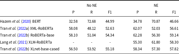
With the growing interest in using machine learning techniques to solve NLP tasks, this approach has also been used for terminology extraction. In Foo (Reference Foo2009), the author proposed learning rules identifying terms, while Hatty et al. (Reference Hatty, im Walde and Bosch2018) classified linguistic expressions using a dense neural network. Later, neural LLMs became more and more widely used to solve the task. In 2020, the TermEval (Rigouts Terryn et al. Reference Rigouts Terryn, Hoste, Drouin and Lefever2020a) shared task was carried out as part of the Workshop on Computational Terminology (CompuTerm). The first competition in term extraction was performed on the ACTER (Annotated Corpora for Term Extraction Research) (Rigouts Terryn, Hoste, and Lefever, Reference Rigouts Terryn, Hoste and Lefever2020b), which contains annotated data in three languages (English, French, and Dutch). This shared task began the era of using learning methods based on annotated data rather than using a set of features that characterize terms. The best results were obtained by the BERT-based model (Hazem et al. Reference Hazem, Bouhandi, Boudin and Daille2020), and it was the first documented use of a transformer-based model to solve the ATE task. The model was trained by giving pairs consisting of a sentence together with a term annotated in it. As negative examples, randomly chosen n-grams were used. The classification of whole n-grams as terms or non-terms is commonly referred to as the sequence classification method, as it categorizes sequences of tokens. Another approach is to classify each token separately and determine whether it is part of a term (token classification). The last method is used, for example, in Lang et al. (Reference Lang, Wachowiak, Heinisch, Gromann, Zong, Xia, Li and Navigli2021),Footnote b Tran et al. (Reference Tran, Martinc, Doucet and Pollak2022a), and Tran et al. (Reference Tran, Martinc, Pelicon, Doucet and Pollak2022b). In our paper, we examine the results of the token classification. In Table 1, we show the results achieved in recent years by some of the researchers who solved the ATE task by sequence or the token classification method using Bert-like LLMs. The results reported in research concerning ACTER are often difficult to compare as authors use various datasets for training (monolingual, multilingual); various test sets (with and without NE); and various methods of evaluation, that is, token-level evaluation (IO or IOB schema) or checking lists of terms. All approaches in Table 1, except the first one, are obtained for token classification. The first three results are given for models trained on English ACTER data, while the last two used multilingual ACTER training data. All results are evaluated on the Gold Standard (GS) list of terms of the ACTER-HTFL dataset. We can see there that the F1 measure was usually a little above 50%. Using BERT resulted in good recall but low precision, while precision and recall were at a similar level for RoBERTa.
The results of ATE evaluated on the list of terms of the ACTER-HTFL dataset in English. The first three results are for models trained on English ACTER data, while the last two are for models trained on multilingual ACTER data
In the ATE task, transformer-based token classification models, hereinafter referred to as transformer-based models for short, obtain results that outperform all traditional methods based on statistics and heuristics. For some data, they achieved an F-measure of more than 0.6 (see the results for Duch in Lang et al. (Reference Lang, Wachowiak, Heinisch, Gromann, Zong, Xia, Li and Navigli2021)), a level which was hard to obtain for the previously used methods. Such a result attracts the attention of the terminology community, so data, similar to ACTER, is now available for the Slovenian language. The RDSO5 (Jemec Tomazin et al. Reference Jemec Tomazin, Trojar, Atelšek, Fajfar, Erjavec and Žagar Karer2021) corpus is used to train a transformer-based tool for the automatic term identification (Tran et al. Reference Tran, Martinc, Repar, Doucet and Pollak2022c) with a similarly high F-measure. An additional advantage of transformer-based methods is their openness to multilingualism, see, for example, (Tran et al. Reference Tran, Martinc, Repar, Ljubešić, Nikola Doucet and Pollak2024), where authors show that cross-lingual and multilingual models outperform results of monolingual models.
Although the results cited above are in line with many others showing that transformer-based LLMs are the best method for solving many NLP tasks, they are far below those obtained, for example, for the popular named entity recognition (NER) task, where the F1 can be above 0.9. We try to find the cause of this discrepancy.
In this paper, we analyze several training-testing scenarios to find features that make the ATE task easier or harder to solve for given texts. To achieve this goal, we examined the results obtained by the transformer-based method in detail. Our focus was not on obtaining a score that improved the current best score but on investigating which types of terms are recognized in which types of texts. Therefore, we use a simple method that makes it easy to reproduce the results, that is, a publicly available algorithm which is trained using a small language model due to the need to conduct many experiments. We have chosen an approach applied in D-terminer (Rigouts Terryn, Hoste, and Lefever, Reference Rigouts Terryn, Hoste and Lefever2022a). The method classifies subsequent tokens annotated in the IOB standard in its context and assesses whether it is a part of a term. The method achieves great results for many tasks and it is the standard approach to the Named Entities Recognition (NER) task (Goyal, Gupta, and Kumar, Reference Goyal, Gupta and Kumar2018). In Lang et al. (Reference Lang, Wachowiak, Heinisch, Gromann, Zong, Xia, Li and Navigli2021) and Rigouts Terryn et al. (Reference Rigouts Terryn, Hoste and Lefever2022b), the method is compared with other approaches, which proves that it performs well. In the last paper, the authors showed that the results obtained by the HAMLET (Rigouts Terryn, Hoste, and Lefever, Reference Rigouts Terryn, Hoste and Lefever2021)—a complex, difficult to reproduce method, which combines traditional statistical features and a supervised machine learning approach to calculate thresholds—are comparable with the new transformer-based approach.
3. Data description
Although the ATE task has quite a long history, there are only a few datasets annotated with terms. The best-known and most commonly used open-domain corpus manually annotated with terminology phrases is ACTER.Footnote c It contains data in three languages: English, French, and Dutch, related to four domains: corruption (CORP), dressage (EQUI), heart failure (HTFL), and wind energy (WIND). In our research, we conducted numerous experiments. To be able to analyze the results and come to conclusions, we focused on one language. We chose English, for which there is also a quite large RD-TEC corpus—The ACL Reference Dataset for Terminology Extraction and Classification, version 2.0, ACL RD-TEC 2.0, (QasemiZadeh and Schumann, Reference QasemiZadeh and Schumann2016). The current version was released in 2022.Footnote d To add even more diversity and test the method on short texts, we annotated three small Wikipedia entries. Below, we look at all the chosen data. Some information is repeated from the original papers.
3.1 ACTER
The ACTER term identification schema is organized around two orthogonal dimensions: lexical (LS) and domain specificity(DS). The annotation is not limited to noun phrases, as is often the case, but adjectival and verbal terms are also considered. Additionally, all NE, both related and unrelated to the given domain, are annotated. The terms belong to one of three categories:
-
• specific term: terms relevant for the given domain, their detailed meaning is only understood by the domain experts (LS + DS+), for example, tachycardia in cardiology,
-
• common term: terms relevant to the domain but understood by a person with general knowledge (LS-DS+), for example, heart in cardiology,
-
• out-of-domain term: terms not specific for the domain, but generally unknown (terms from the other domain, LS + DS-), for example, p-value in cardiology.
The first two categories are usually assumed to be domain terms, but sometimes the third class is also taken into account. As this class is much less numerous, this does not alter the results substantially. In most experiments on ACTER reported in the literature, NE were also treated as terms.
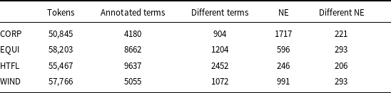
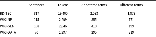
It has been widely observed that identifying domain-related terms in text is not an easy task, mainly because of the many borderline cases. When the annotation is carried out on longer texts, keeping the annotations consistent is the additional problem. For the ACTER data, a quality check was carried out on part of the corpus. The difficulty of the task was confirmed, as the Kappa coefficient describing annotators’ consistency counted on a selected subset of data was relatively low—0.59 (Rigouts Terryn, Hoste, and Lefever, Reference Rigouts Terryn, Hoste and Lefever2020b). Just one person annotated the entire dataset, so its consistency and completeness could not be very high. It might be a problem when we use this data as a training set, but for evaluation, when we are mainly interested in a list of terms, it is less crucial. The basic statistics of this corpus are shown in Table 2.
ACTER data statistics: number of tokens, number of annotated terms, number of different terms, annotated named entities (NE), and different NE
The ACTER texts are annotated in two different styles. There is an in-line annotation that indicates the beginning and the end of each term. Both single-word and multi-word sequences are annotated, and internal terms are also labeled. These annotations were the source for preparing the list of terms which were identified in every language-domain part (so-called GS lists). The second type of annotation is a token-based annotation in two IOB and IO variants. No nested terms are accounted for. We used IOB-annotated files in our work.
3.2 ACL RD-TEC
The RD-TEC corpus was developed to provide a benchmark for the evaluation of term and entity recognition tasks based on specialized texts from the computational linguistics domain. It consists of 300 abstracts from articles published between 1978 and 2006 in which both single- and multi-word LS units with a specialized meaning are manually annotated by two annotators. Several classes of terms are identified in this corpus, but we treat them all as one class, together with domain-related NE annotated within the data using the same labels as other terms. For our experiments, we selected a subset of this corpus containing 171 abstracts whose annotations were agreed upon by both annotators. Data statistics are given in Table 3.
Other data statistics

3.3 Wikipedia articles
To check the results that the method can achieve on relatively short texts, we prepared a small corpus containing three Wikipedia articles defining specialized terms from different domains.Footnote e The selected texts concerned: noun phrase (WIKI-NP), genotype (WIKI-GENE), and data structures (WIKI-DATA). The texts were annotated using ACTER annotation instructions by two of the coauthors of this paper and then underwent a verification phase aimed at obtaining a coherent GS. Both annotators are experts in the areas covered by the articles on noun phrases and data structures, but they have only general knowledge of genetics. The Kappa coefficient calculated on the token level for the maximum term span was equal to 0.77 for WIKI-DATA, 0.71 for WIKI-GENE, and 0.86 for WIKI-NP. The main differences concerned the choice between specific and common terms and between common terms and non-terms. When the decision was binary (term, no term), Kappa was equal to 0.86, 0.83, and 0.91, respectively. Data statistics are given in Table 3.
4. Evaluation methods
An important factor when choosing a method of evaluation is the format of the results provided by ATE. Traditional ATE methods deliver a list of terms. Evaluation is then performed based on a comparison of the obtained list of phrases with a GS list of terms. Evaluation of a method involving the assignment of IOB (or IO) labels to tokens (e.g. a transformer-based method) can be performed at a token level when the correctness of the label assignment is assessed. These two approaches are not easily comparable, as it is necessary to transform one form of the result into another.
If a result is given as a list of terms and we want to evaluate them on the token level, then all occurrences of terms in the text should be labeled with ‘B’ and ‘I’. A problem arises when a result list contains nested terms that never occur in text as stand-alone phrases, as they cannot be represented in an IOB annotation. Additionally, traditional ATE methods usually give terms in normalized forms, which would result in assigning all forms of terms in texts.
Reverse issues occur when generating a list of terms from an IOB annotation. The IOB (or IO) annotation, resulting from transformer-based methods, does not make it possible to code nested terms. Thus, if a term has not appeared as a maximum phrase, it will not appear in the list of terms. Secondly, only certain forms of a normalized term are recognized by the method, which raises the question of whether one recognized form allows us to assume that all forms are recognized. For example, some of our models recognized only the plural form shunts in HTFL, while both forms shunt and shunts are manually annotated. Is it enough to decide that the term shunt, in its normalized singular form, is recognized?
In this paper, in accordance with the solution adopted in ACTER, we use evaluation based on the GS list of terms. Since we are extracting the list of terms from the annotated data, we only include terms that occurred in the text as a tagged maximum phrase. That is, if a phrase always occurred as a fragment of a broader annotated phrase, it is not included in our GS. The differences between these lists are negligible.Footnote f Usually, more examples are not found in the annotated data than those not found on the original GS list. It should also be noted that the lists contain all phrase forms as separate terms, so blood flow, blood-flow and cardiac death, cardiac deaths are different terms.
5. Preparation of language models
In order to conduct our terminology extraction experiments, we prepared several LLMs. We fine-tuned the RoBERTa (Liu et al. Reference Liu, Ott, Goyal, Du, Joshi, Chen, Levy, Lewis, Zettlemoyer and Stoyanov2019) base model on English subsets of the ACTER sequentially annotated texts with IOB labels to perform the token classification task. The selected method is a variation on the one described in the Huggingface documentation of token classification with transformers.Footnote g Essentially, it differs only in the choice of input model and the set of labels. We trained each model for 50 epochs, evaluating the model after each epoch and ultimately allowing the training module to select the one with the best performance, according to the loss function. A batch of four examples for training and evaluating was used. We set the learning rate to 2e-5, the weight decay to 0.01, and the warm-up ratio to 0.2.
First of all, we checked the performance of the generated models on ACTER itself. In generating the subsequent LLMs, we separated one of the four parts of ACTER (CORP, EQUI, HTFL, or WIND) as the test dataset, randomly dividing the remaining data into the training dataset and the validation dataset in a proportion of 90/10, respectively.Footnote h We considered two versions of ACTER annotation—one where specific, common, and out-of-domain terms were annotated, and another where NE were also annotated. We trained two classes of models, that is, with and without NE. The other (non-ACTER) datasets were tested using two models (with and without NE) trained on the entire ACTER data (with the same 90/10 ratio of training to the validation part).
6. Results
6.1 ACTER data
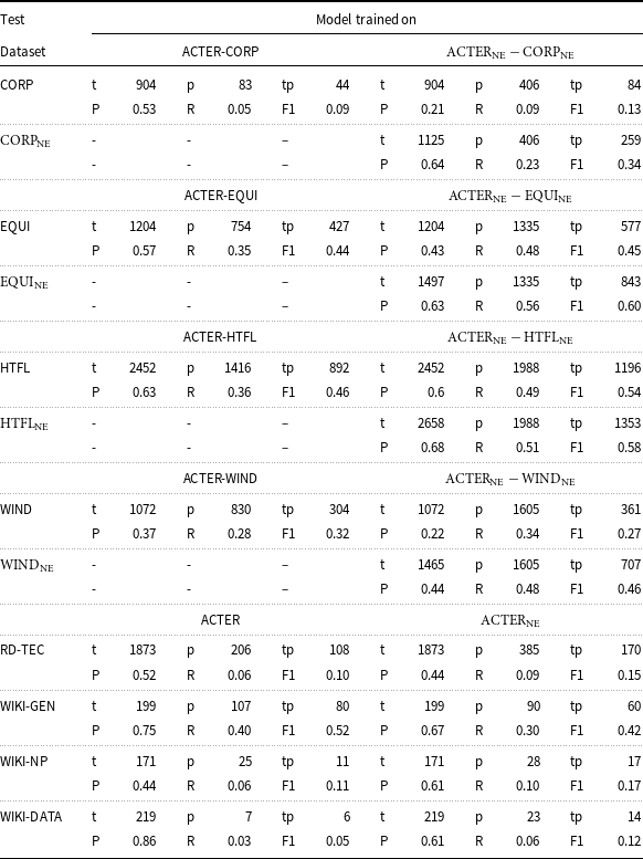
Most of our experiments were performed on the ACTER data, which is most frequently used to train ATE models. However, we did not limit our focus to the almost always used configurations where NE were considered as terms. We show that when we exclude NE (which can be relatively easily identified), the results are much lower. Table 4 contains the results obtained by our models for the ACTER data, in which every three parts are treated as the training data and the fourth as the test data, and it shows substantial differences in the results obtained in such scenarios. Both variants, with NE included and without them, were tested. We adopted the following convention: the names of datasets in which NE are treated as terms that have ne in subscripts, and the names of models are derived from the names of the datasets on which they were trained. When three of the four ACTER parts have been used as a training set and the fourth part (X) is used for testing, the model is called ACTER-X.
Results obtained by our models. The upper part of the table shows models that were trained on three parts of the ACTER corpus (the part which was removed is noted in the rows as a subtracted one, e.g. ACTER-CORP, and tested on the fourth (listed in the first column). The models were trained in two variants: using only term annotations or using term and named entities annotations. The lower part contains the results obtained for the RD-TEC corpus and three Wikipedia entries, by the model trained on the entire ACTER corpus. Notation: t – number of terms annotated in the corpus, p – number of terms predicted by the models, tp – number of correct predictions. P – precision, R – recall
We tested our models at the term levelFootnote i using the list of correct terms obtained from the annotated corpus. We also performed evaluation at the token labels level, considering only tokens annotated as elements of terms (i.e., the B and I label), and the results were very similar, so we have not included them here.
The first experiment was carried out according to the rules of the TermEval shared task, when the HTFL data was used as the test set. The results of F1 = 0.46, 0.58 for identifying terms or terms and NE by models trained respectively on data with and without NE were similar to the best results reported at the TermEval Workshop (0.45, 0.47). For a terminology extraction task, such values are considered high. When we repeated the same experiment, choosing different parts as the test set, we received similar results for EQUI (0.44, 0.6), and slightly lower ones for WIND (0.32, 0.46). But for CORP data, the results for the terms without NE deteriorated substantially to F1 = 0.09.Footnote j The results do not even include a term that characterizes the entire set, that is, corruption, which occurred 300 times in the data. Adding NE to the training and test data substantially improved the results to 0.34. To verify whether the performance improvement is mainly due to NE recognition or whether the addition of NE annotation helps with term recognition, we tested models trained on both term annotation and NE on data where only terms were annotated. As can be seen in Table 4, this approach improves recall while lowering precision. For the three test sets with relatively good results, the overall change measured by F1 was not uniform: for the HTFL data, we see a significant improvement (F1 is higher by 0.08); for EQUI, the results are almost the same; while for WIND, they are worse by 0.05. For the CORP data, the results improved by 0.05, but still remained very low (0.13). Given the similar size of all parts, such a difference indicates that there are certain properties of the data that affect the effectiveness of the method. In the remainder of this article, we will examine some of these properties and their possible impact on the results.
6.2 Other data
We used other data, that is, RD-TEC and three Wikipedia entries, to see how the models behave on texts of different length and structure (RD-TEC contains abstracts, so the frequency of terms in the text is higher) and annotated by different people. We used models trained on all four ACTER datasets in the experiments.
In the case of RD-TEC (see Table 4), we obtained F1 = 0.10 for the model trained on the data without NE. This result improved slightly (F1 = 0.15) when NE were included during model training.
The results for three Wikipedia entries are also shown in Table 4. The very good (F1 = 0.52) result is obtained for the genotype (WIKI-GEN). In this case, adding NE to the training set made the results worse. The results for noun phrase (WIKI-NP) and data structures (WIKI-DATA) are very poor. Here, adding NE helped, but not very much. For both texts, the problem is the very low recall at a level of about 0.1 or less. An interesting observation is that for the genotype data, both precision and recall are higher than for most of the other classes, while for data structures, the recall is very low—only 7 terms were identified, 6 of them were correct. For the model trained with the NE, these changed slightly to 23 and 14.
6.3 Checking different language models
In order to test whether the results depend on the specific language model used, we repeated a large part of the experiments described in the previous section, selecting other variants of BERT-like models: RoBERTa large, BERT (Devlin et al. Reference Devlin, Chang, Lee, Toutanova, Burstein, Doran and Solorio2019) in four variants—basic/large and cased/uncased, DeBERTa (He et al. Reference He, Liu, Gao and Chen2021) base, and MPNet (Song et al. Reference Song, Tan, Qin, Lu and Liu2020) base.
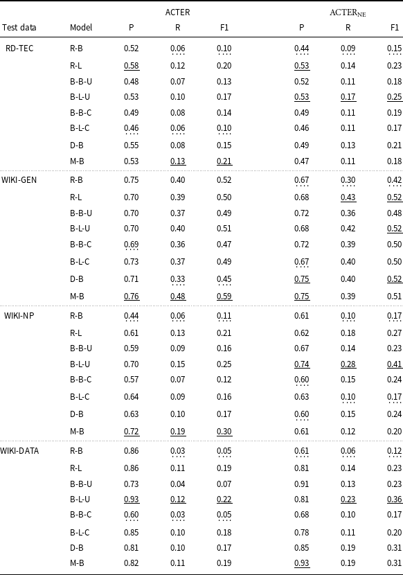
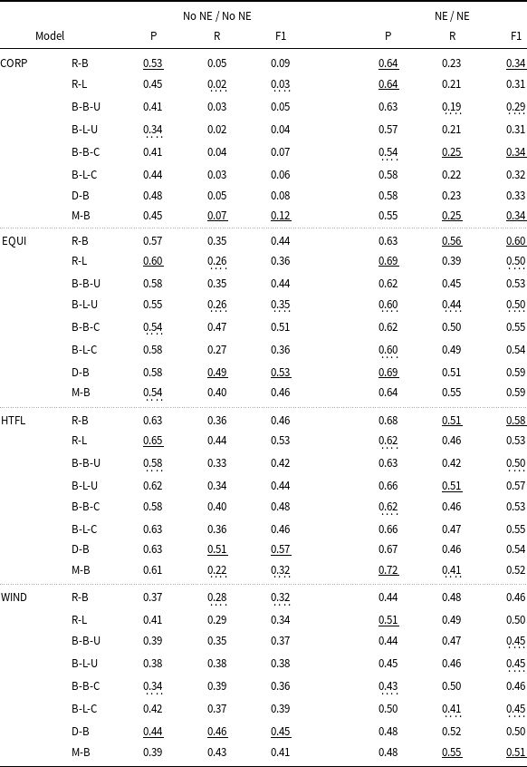
Of the three configurations tested previously, we chose two: training and testing on data consistently with and without named entity annotations. The results obtained for the different models (see Tables 5 and 6) obviously vary, but the differences are not substantial and the performance levels on the different test sets are similar. For the ACTER data, all models gave the worst results on the CORP test set, while for the other sets, the results obtained by F1 ranged between 0.32 and 0.57 for data without NE and 0.45 and 0.6 for data with NE. The differences between the results were usually not greater than 0.1, with a few exceptions, for example, the very low recall for the HTFL data obtained by the MPNet model for data without NE. For the other four datasets, the best results were consistently obtained for WIKI-GEN data. For the remaining three sets, the recall was quite low (between 0.1 and 0.2). Precision for all four sets was much better, ranging from 0.58 to as high as 0.93 for WIKI-DATA, but with such low recall, these high values are misleading. Since, in general, the differences between the results obtained using different LLMs were not very large, and the best results were obtained using different models for different datasets, we decided to run the rest of the experiments using a relatively small RoBERTa base model to make our experiment less computationally expensive.
Comparison of results for different models tested on the ACTER corpus. The first column contains the names of the corpus parts on which the models were tested. The second contains the names of the models being tuned: RoBERTa base (R-B), RoBERTa large (R-L), BERT base/large cased/uncased (B-B-C, B-B-U, B-L-C, B-L-U), DeBERTa base (D-B), and MPNet base (M-B). All these models were trained on the remaining three parts of ACTER. The remaining columns contain precision, recall, and F1 for the models trained and tested on data with and without named entities, respectively. The best result for each data configuration is underlined, the worst is highlighted with a dashed line

Comparison of results for different models tested on the RD-TEC corpus and three Wikipedia articles. The names of the models are explained in Table 5. These models were trained on the entire ACTER corpus both on data with and without labeled named entities
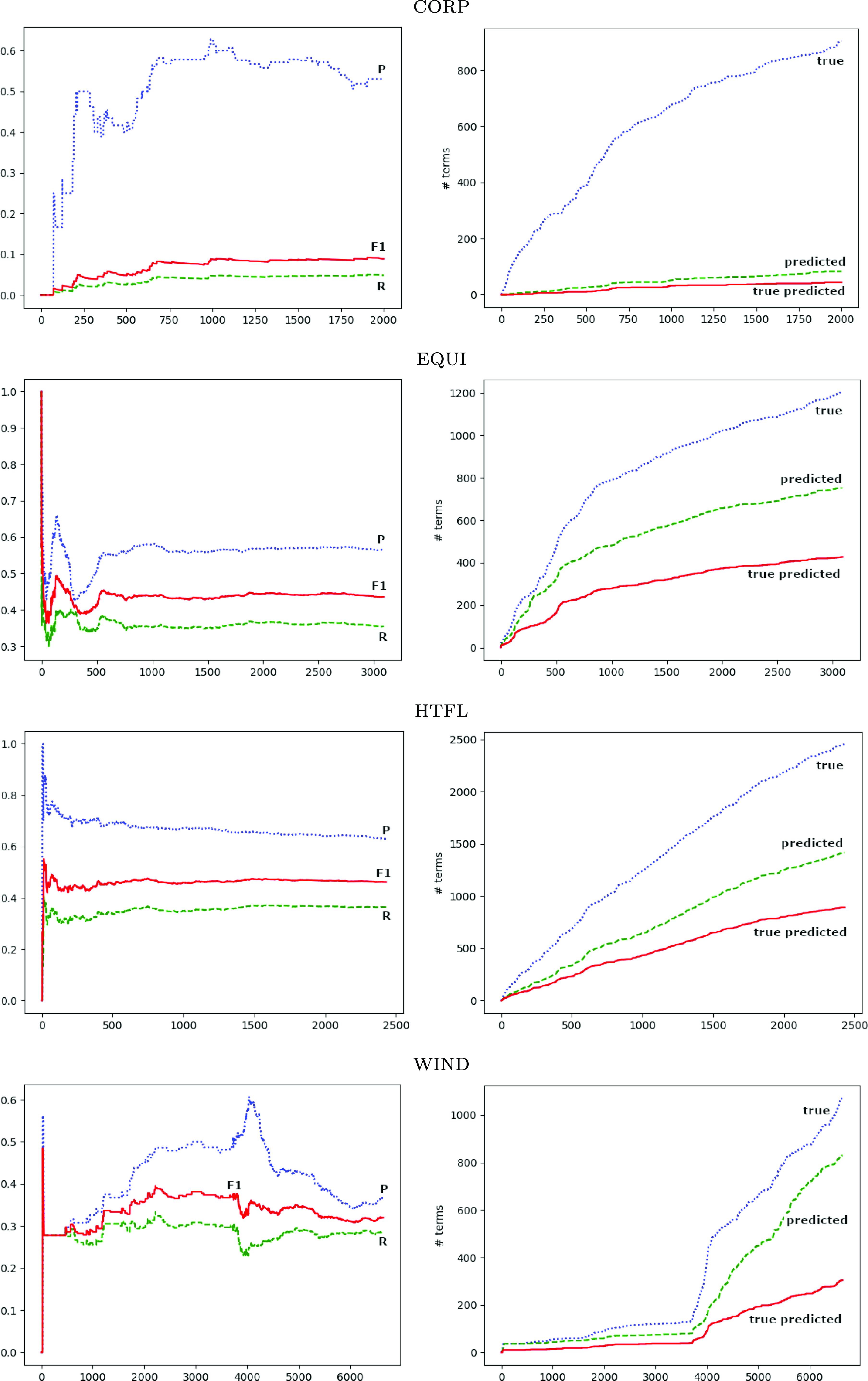
6.4 ACTER: incremental analysis
Section 6.1 gives the final results when the list of extracted terms is evaluated. As only some term occurrences are recognized by the method, the graphs in Figure 1 show how precision (top blue graph), recall (bottom green graph), and F1 score (middle red graph) change as successive sentences are analyzed for the ACTER corpora. In each point, the evaluation was made against a list of terms annotated in the analyzed part of the text, so ideally, both precision and recall should be equal to 1. The datasets used for training and testing did not include NE.
The results for the HTFL and EQUI corpora show that for the initial sentences, the measures can change substantially as sentences are added, but after 500 or 750 sentences of the respective data, the results stabilize. The WIND data is clearly different, so probably the numerous tables in the text cause variability in the number of new terms introduced and those correctly recognized. The number of terms detected for the CORP data is too small to analyze.
7. Corpora properties
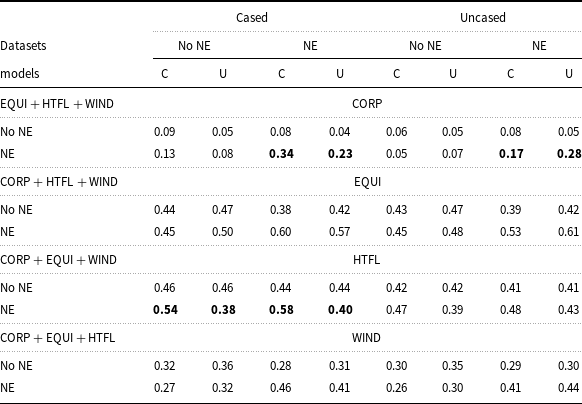
7.1 Case sensitivity
A simple but important feature of text is the fact that the same words occur in capitalized text and in lowercase. While capitalization is important for recognizing NE, it is not clear if it has any influence on the results of terminology extraction. To check this, we trained both cased and uncased models on the appropriate versions of the ACTER corpora. A comparison of the results obtained by the cased and uncased models did not provide a clear answer as to which is better suited for terminology extraction. We compared the performance of cased and uncased models on cased and uncased datasets of ACTER. Extracted terms (and NE) have been converted to lowercase, as is customary in ACTER. When comparing the performance of two models, we checked their F1 scores rounded to two decimal places. We considered the model with the higher F1 score to be better. Models with the same F1 scores can be said to be equally good (or bad). The results of the comparisons are shown in Table 7. It turned out that cased models performed a little bit better on CORP and HTFL, while uncased models were slightly better for EQUI and WIND.
Incremental analysis for ACTER corpora. On the left are the results for precision (P), recall (R), and F1 score, and on the right are the numbers of true, predicted, and true predicted terms after examining consecutive sentences.
Comparison of F1 scores, rounded to two decimal places, obtained by cased (C) and uncased (U) models tested on the same datasets. If these scores differ by at least 0.1 for the same data, they are highlighted
7.2 POS schemata
Table 4 demonstrates a predictable improvement in performance when models are trained and tested on datasets that include NE, as these are generally easier to identify compared to terms. However, adding named entity annotations to the training data also improved term recognition when testing on data that did not include NE (reported previously in Rigouts Terryn (Reference Rigouts Terryn2021)). Only in one case—WIND—did we see a decrease in performance. This suggests that incorporating annotations for similar, albeit distinct, types of concepts can sometimes increase recall to a degree that outweighs a potential decline in precision, resulting in better overall outcomes. To further explore this direction, we decided to look for other possibilities to extend training data. It was previously observed that terms generally have a very typical syntactic structure, thus, POS sequences were used to select term candidates or as a feature to improve candidates’ scoring (Rigouts Terryn et al. Reference Rigouts Terryn, Hoste and Lefever2021). As this information is easily obtainable by using taggers, we decided to check whether annotating as terms the random sequences with typical POS patterns for terms would also improve the results.
First, we checked the POS sequences of all annotated terms within the ACTER corpus (Rigouts Terryn, Hoste, and Lefever, Reference Rigouts Terryn, Hoste and Lefever2020b). As expected, the most common of these are single nouns, but there are other common patterns, the most frequent of which are adjective-noun and noun-noun pairs. Single adjectives were also quite often treated as terms. The top five POS schemata in all datasets are similar, the greatest exception is the two-nouns pattern (not the single-noun pattern) being the most frequent one in the WIND data. Among predicted terms, the diversity of patterns is much lower and in all sets, the single-noun pattern is the most common. Very few results for the CORP data are mainly single-word terms. For the other three sets, the top POS pattern distribution is similar to the original data.
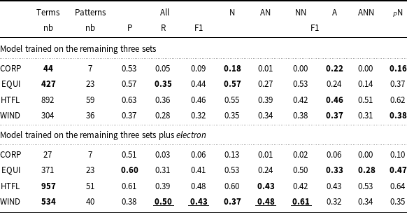
To test our hypothesis, we chose one more entry from Wikipedia, electron, which has around 10K tokens and represents a domain different from those already existing in the ACTER corpus. We tagged it using Stanza (Qi et al. Reference Qi, Zhang, Zhang, Bolton and Manning2020) and annotated as terms a random 50% of all the sequences that have tag patterns identical to one of the six most frequent term POS sequences in ACTER (see Table 8 for the list). This process resulted in 1768 annotations. As in the previous experiments, the models were trained on the three parts of the ACTER corpus (without NE) plus this additional file, and tested on the fourth part. Table 8 shows the values obtained with and without this additional training set. The variants that are at least 3% better are in bold, and those at least 10% better are additionally underlined.
Results for terms with the specific POS sequence using the original training data and data extended by the electron entry. Abbreviations used: N-noun, A-adjective, $_{P}$
N-proper noun. The number of true predicted terms and the different syntactic patterns they represent are given in columns 2 and 3
$_{P}$
N-proper noun. The number of true predicted terms and the different syntactic patterns they represent are given in columns 2 and 3

Upon analyzing the results, we can see that they are not uniform, indicating that the poor performance of the models is not caused by the lack of information about typical syntactic patterns of terms. Interestingly, for three of the datasets, results remained relatively stable (changes ranging from −3% to + 2%). However, for the WIND dataset, there was a notable improvement, with an increase of 0.11 in the F1 score, coming from a 0.22 rise in recall, which, surprisingly, was not accompanied by any loss in precision. About 230 more terms were correctly identified. This improvement can be attributed to the enhanced identification of two-word terms composed either of an adjective and a noun or two nouns. These substantially different results may be linked to the previously mentioned observation that terms consisting of two nouns are the most common in the WIND dataset. The addition of examples with this POS sequence, less frequent in other datasets, may have contributed to the increase. It should be noted that the WIND part was the only one in which adding NE lowered the results. To check the possible source of that improvement, other than POS annotation, we looked at the overlap between our randomly annotated terms within the text about an electron and the terms annotated in the WIND data. It turned out that these term lists have 126 common words, which led to the correct recognition of 49 one-word terms. This number is much lower than the number of newly correctly recognized terms (230), so in this case, the additional data led to a real improvement in term recognition.
7.3 Frequency
In many studies on ATE, the statistical distribution of corpus words is used as an important feature for term selection (see e.g. Yang, Reference Yang1986; Damerau, Reference Damerau1993; Manning and Schütze Reference Manning and Schütze1999). The ratios of relative frequency between corpora have been applied for identifying terms (Chung and Nation, Reference Chung and Nation2004) or filtering out phrases that are not domain-specific (Navigli and Velardi, Reference Navigli and Velardi2004).
Token frequency is an important feature in term recognition that LLMs can use for this task. Therefore, we examined ACTER corpora and checked how often words from these corpora are used in a corpus of general English. To count the average frequency of tokens, we used data from the Trillion Word Corpus (TWC) created by Google from public web pages.Footnote k This data contains the 333,333 most commonly used single words on the English language web and gives forms which occurred more than 12711 times, while the most frequent English word the occurred 23,135,851,162 times. Stop words constitute a substantial percentage of tokens in the corpora and have the highest frequency, so we decided not to include them when calculating the average frequency of tokens. For this purpose, we used the list of English stop words provided in the NLTK package.Footnote l The problem that needed to be solved was how to count frequency for terms containing hyphens. The solution we adopted was to check the frequency of the whole token if it could be found in the TWC dictionary. If it was not in this dictionary, we checked the frequencies of the token parts made after dividing the token by hyphens and assuming their average value.
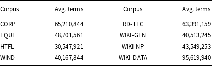
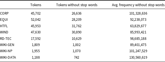
Table 9 shows the number of tokens and their average frequency in the general corpus, counted according to the procedure described above. The ACTER results show that vocabulary in the CORP corpus (corruption data) is mostly general, while the HTFL corpus (heart failure) contains the most specific vocabulary. This conclusion is consistent with the intuition of language users because texts about corruption are typically press reports, unlike descriptions of HTFL therapies. The same Table 9 shows the average frequency in the other datasets. The average frequencies for WIKI-NP and WIKI-DATA are similar or higher than those in the CORP data, and the results of term extraction are poor for these two datasets. Similarly, poor results are for RD-TEC for which the average frequency is also relatively high.
Average frequency of tokens different from punctuation marks counted for tokens without stop words. The first column indicates the number of tokens different from punctuation marks including stop words, while the second one shows the number of tokens without them

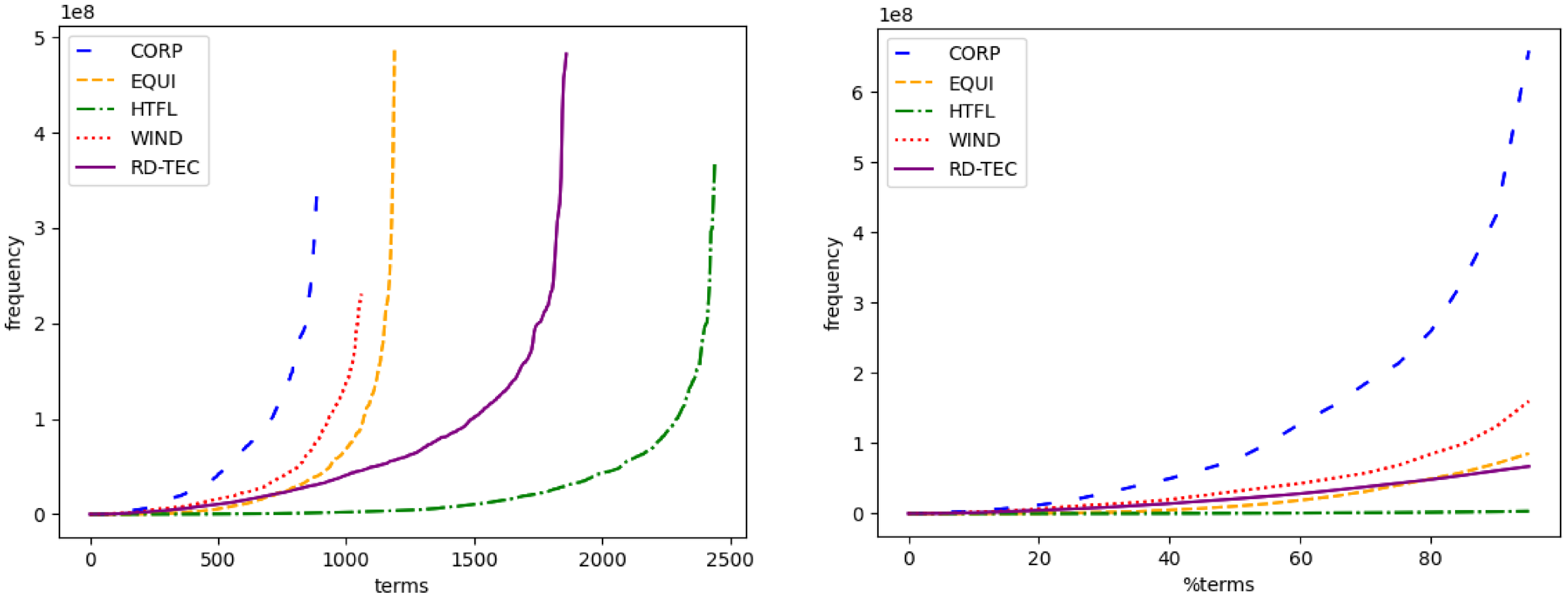
A high average frequency of text does not necessarily imply a list of high-frequency terms, so we analyze the list of manually annotated terminology phrases. For each term, we count its frequency as the average of token (not including stop words) frequency in TWC. Figure 2 shows term frequency for the large datasets, that is, the ACTER corpora and RD-TEC. The left graph shows that for the ACTER corpora, each line contains a shorter or longer segment of relatively rare terms, while the size of a set of very frequent terms is similar for each corpus. At the same time, the RD-TEC term frequency increases fairly quickly. The right graph shows that the percentage of frequent terms is highest in the CORP data. For the RD-TEC corpus, the graph looks different as it is almost a line. Note that this data is significantly different from the ACTER datasets. The corpus is almost three times smaller, while the number of different terms is similar. The density of terms in the text is therefore higher, and the frequency of term repetition is lower.
The average frequency of the list of terms without NE in the corpora counted without stop words is given in Table 10. Among the ACTER corpora, the CORP corpus has the smallest number of rare terms, that is, terms in this corpus are relatively more frequent than in the others. The rarest terms are in the HTFL corpus. For the other datasets, WIKI-GEN has the rarest terms and the best results. The average frequency of WIKI-NP terms is relatively low, and the F-measure is low, too. RD-TEC and WIKI-DATA have frequent terms and poor results.
Average frequency of the list of annotated terms in the corpora counted without stop words
Frequency (according to TWC) of manually annotated different terms of ACTER and RD-TEC data. The left graph displays the frequency according to the number of terms, while the right graph displays the frequency according to the percentage of terms in the datasets.
7.4 Common part of vocabulary
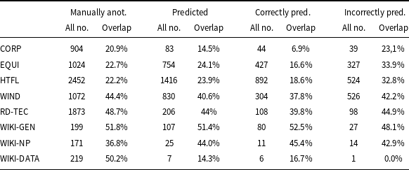
In many NLP tasks, learning-based methods often take advantage of the co-occurrence of tokens in training data and labeled data. It is therefore interesting to see what (if any) relationship exists between the labeled terms/tokens in the training data and the results predicted for a test corpus. To do this, we compare how many terms labeled by the language model contain tokens labeled as part of the term in the training data for each set of the training (and validation) corpora and the test corpus. For an ACTER corpus, we check overlap with the three other ACTER corpora, while for the RD-TEC and the WIKI data, we check overlap with all ACTER corpora.
The results are given in Table 11. For each corpus, we show the number of manually annotated terms; predicted by the model; and those predicted correctly and incorrectly, together with the percentage of terms containing a token tagged as a fragment of a term in the relevant training corpora. The terms containing such tokens we henceforth refer to as overlapping. Stop words are excluded from this counting, so if the only overlapping token for a term is of, it is not taken into account. We only compare whole words, we do not divide them into smaller parts, on which models such as BERT operate. In this comparison, we also do not recognize derived forms of words such as plurals, adjectives, or verbs. For example, the following forms are not joined: constructions, constructed, constructing with the construction form. The table shows that for ACTER and RD-TEC corpora, the percentage of incorrectly recognized overlapping terms is much greater than the percentage of overlapping terms for correctly recognized terms. This may indicate that tokens included in the terms of the training corpora are a positive premise for the term-recognizing models. In the case of the analyzed corpora, this leads to an increase in the number of phrases incorrectly indicated as terms, as the domains of ACTER corpora are not related. The WIKI data is small, so it’s hard to make statistical conclusions from it.
Percentage of terms (columns overlap) containing a token tagged as a fragment of a term from another domain. The columns headed all no. indicate the number of all terms. Statistics are given for terms annotated manually, all predicted by the model and those predicted correctly and incorrectly by the model

For each domain except WIKI-DATA, we provide examples of incorrectly identified terms along with the training domain from which they originate:
-
CORP: tests (EQUI); follow-up (HTFL); network, technical (WIND)
-
EQUI: illegal, criminal penalties (CORP); admission, blood, breathing, chest, emergency room, hospitalisation (HTFL); power, mechanisms, energy (WIND)
-
HTFL: cost, economic, financial (CORP); leg, pacing, relaxation, training, walk (EQUI); electric, electrical, flow, mechanical (WIND)
-
WIND: business, contract, economic, enforcement, public interest (CORP); arms, exercise, thrust (EQUI); baseline, significantly, health (HTFL)
-
RD-TEC: judges, laws (CORP); air, train (EQUI); correlation, randomized (HTFL); empirical, industry, machine, meteorological (WIND)
-
WIKI-GEN: epigenetic, genetic, hereditary, correlated, proteins (HTFL); technology (WIND)
-
WIKI-NP: election, government, economic (CORP); energy (WIND)
The examples above show that, except for the WIKI-GEN data, these terms are from outside the domain of the corpus under consideration. Since WIKI-GEN and HTFL domains are relatively similar, the terminology in HTFL somewhat supports the recognition of WIKI-GEN terms. 38% of WIKI-GEN terms overlap with HTFL terms. Of the 22 terms predicted in WIKI-GEN and being terms in HTFL, 16 are correctly predicted as terms and five are incorrectly predicted. All of them are included in WIKI-GEN broader phrases annotated as terms. The correctly predicted 16 terms are the only common terms in both datasets (all are one-word terms).
User intuition and experiments with filtering out general terms using terminology from another domain (Drouin, Reference Drouin, Lino, Xavier, Ferreira, Costa and Silva2004) indicate that for unrelated domains, the overlap of entire terms is a marginal phenomenon. This is different for related domains, such as veterinary medicine and human medicine, where many terms are common. Therefore, when selecting both training and validation data, attention should be paid to the relatedness of the vocabulary.
8. Consistency of results
8.1 More data does not mean better results
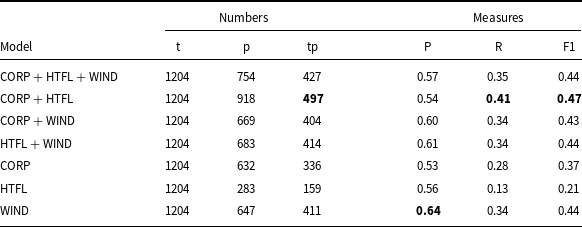
In this section, we analyze results for models obtained for all configurations or data tested on EQUI without named entity annotations. The models were also trained on data without these labels. We have chosen this dataset because it has less specific vocabulary (see Sec. 7.3 ) and the results are similar to those in HTFL, for which we obtained the best results (see Tab. 4).
The results in measure values and numbers of terms are given in Table 12. The best results are in bold, so the best F1 measure is for the model trained on the CORP + HTFL data. The F1 measure for three models: CORP + HTFL + WIND, HTFL + WIND, and WIND is the same and equal to 0.44. Note that the highest precision among these three models is achieved for the model trained solely on the WIND data. This is therefore an unpredicted outcome, as we expected that the results obtained by a model trained on smaller data would be noticeably worse.
Results obtained by models on the EQUI data. The best results are in bold. Notation: t – number of terms annotated in the corpus, p – number of terms predicted by the models, tp – number of correct predictions. P – precision, R – recall
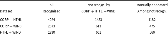
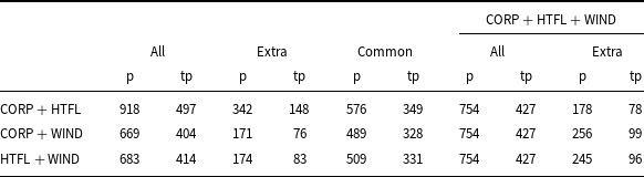
A deeper analysis of the results shows significant differences in the composition of term lists recognized by models trained on smaller and larger datasets, see Table 13. It shows that more than a quarter of the terms (for the CORP + HTFL, even 37%, i.e. 342 out of 918) recognized by the models trained on two selected ACTER datasets are not recognized by the model trained on CORP + HTFL + WIND. A comparison of the results of the CORP + HTFL (the best F1 measure) and CORP + HTFL + WIND models shows that results obtained by the much larger amount of training data do not contain as many as 342 terms (148 of which were correct). Note that this is almost half of the terms predicted by the model trained on CORP + HTFL + WIND data, that is, 754 terms, and more than one-third of correctly predicted terms (427).
Comparison of the term lists obtained by models trained on two datasets with the model trained on all datasets except EQUI. The columns headed all give the number of all terms; the columns headed extra give the number of extracted terms that are not common to compared lists; the column headed common gives the number of common terms recognized by both compared models; p – numbers of predicted terms; tp – numbers of true predicted terms

A comparison of lists of predicted phrases shows that 329 terms are indicated by all four models discussed above. 239 of them are correctly recognized as terms. Among them are phrases that are not only very specific to the domain, for example, dressage, horse, horse riding, bridle, equestrian, equestrianism but also more general phrases, for example, core, front end, gymnastic. 70% of correctly recognized terms are single words and only two phrases contain three words: driving leg aids and outside leg aid. 16 terms were recognized by all models trained on the smaller datasets and not recognized by the CORP + HTFL + WIND model (e.g., breeches, dressage saddle, while 20 terms were only recognized by the last model (e.g., riding horse, cavalry). The list of terms not recognized by all four models consists of 559 terms, which is 46% of the total of manually annotated terms.
The fact that the list of recognized terms has changed does not necessarily mean that the addition of new training data has resulted in the previous terms not being recognized. It is theoretically possible that the previously recognized term is now part of a longer term. So to give a complete picture of what happens when the training data is expanded, we check how many tokens recognized as components of terms in a model trained on smaller datasets receive the label ‘O’ (out of terms) in the CORP + HTFL + WIND model. We also check how many of these tokens are correctly indicated as term elements in the manually annotated data. The numerical outcomes are given in Table 14. Around one-third of tokens recognized as term components by the model trained on smaller data are neglected by the model trained on CORP + HTFL + WIND. The difference in recognized terms is therefore not due to the recognition of longer terms by the larger model.
The number of tokens recognized as a term component (labels: ‘B’, ‘I’) by the models trained on the dataset and not recognized by the model trained on CORP + HTFL + WIND. The column headed all recognized gives the number of tokens recognized as a term component by the model in dataset. The next column gives the number of tokens recognized by the smaller dataset and not recognized as term components by the model CORP + HTFL + WIND. The last column gives the number of tokens manually annotated as a term component within those in column 3
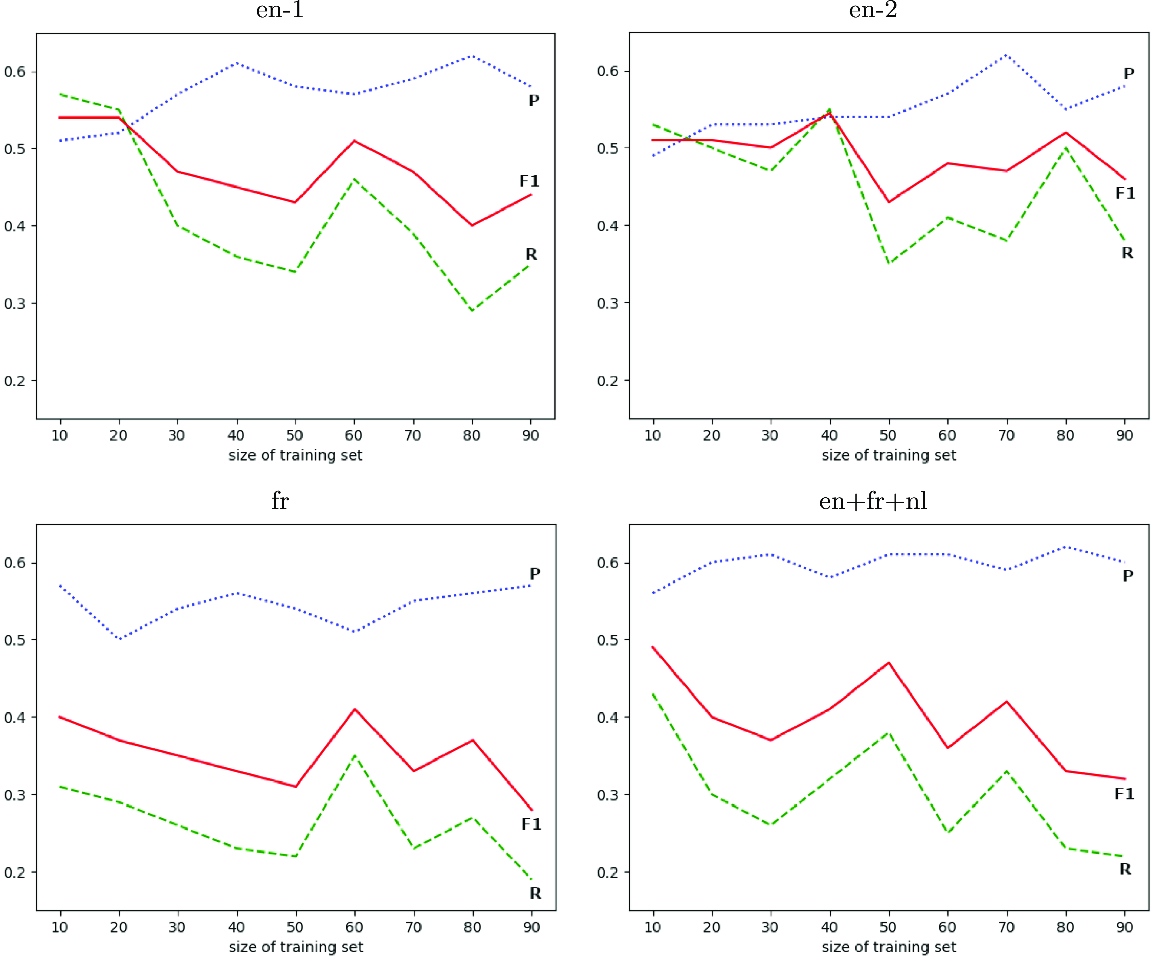
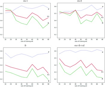
Precision (P), recall (R), and F1 score obtained by nine models tested on the EQUI dataset and trained on nine sets successively increased by 10% of the data from each of the other parts of the ACTER corpus for four experiments: with English (en-1, en-2), French (fr), and multilingual (en+fr+nl) texts.
To show that more data does not lead to better results, we performed one more experiment consisting of:
-
• dividing each of the CORP, EQUI, and HTFL datasets into ten equal, randomly selected subsets: $\textrm {CORP}_i$
,
$\textrm {HTFL}_i$
,
$\textrm {WIND}_i$
, for
$0 \leq i \lt 10$
,
$\textrm {CORP}_i$
,
$\textrm {HTFL}_i$
,
$\textrm {WIND}_i$
, for
$0 \leq i \lt 10$
, -
• establishing
$\textrm {CORP}_0 +\textrm {HTFL}_0 +\textrm {WIND}_0$
as the validation dataset, -
• training nine subsequent models on
$\sum _{1}^{i} \textrm {CORP}_i +\textrm {HTFL}_i +\textrm {WIND}_i$
, for
$1\lt\, = i \lt\, = 9$
, -
• and testing them on the EQUI corpus.


This experiment was repeated with two randomly selected subsets $\textrm {CORP}_i$
,
$\textrm {CORP}_i$
, $\textrm {HTFL}_i$
and
$\textrm {HTFL}_i$
and $\textrm {WIND}_i$
for English language texts and also for French and multilingual texts. To create the models for French and multilingual texts, we used the CamemBERT (Martin et al. Reference Martin, Muller, Ortiz Suárez, Dupont, Romary, de la Clergerie, Seddah, Sagot, Jurafsky, Chai, Schluter and Tetreault2020) base and XLM-RoBERTa (Conneau et al. Reference Conneau, Khandelwal, Goyal, Chaudhary, Wenzek, Guzmán, Grave, Ott, Zettlemoyer, Stoyanov, Jurafsky, Chai, Schluter and Tetreault2020) base models, respectively. The results of these experiments are shown in Figure 3. We can see there that all measures are very unstable. Adding another 10% of the training data sometimes improved, but sometimes significantly worsened, the results. The most surprising outcome is that, in some cases, the best results are obtained when training on the smallest number of examples (10% of data). In all four experiments, these results were better than those obtained using 90% of the data. We can also easily see that in most cases, the precision of the method was better than its recall. The decrease in recall when increasing the size of the training set is clear evidence that providing a language model with only annotated sentences as training data is insufficient to create a good term recognition model.
$\textrm {WIND}_i$
for English language texts and also for French and multilingual texts. To create the models for French and multilingual texts, we used the CamemBERT (Martin et al. Reference Martin, Muller, Ortiz Suárez, Dupont, Romary, de la Clergerie, Seddah, Sagot, Jurafsky, Chai, Schluter and Tetreault2020) base and XLM-RoBERTa (Conneau et al. Reference Conneau, Khandelwal, Goyal, Chaudhary, Wenzek, Guzmán, Grave, Ott, Zettlemoyer, Stoyanov, Jurafsky, Chai, Schluter and Tetreault2020) base models, respectively. The results of these experiments are shown in Figure 3. We can see there that all measures are very unstable. Adding another 10% of the training data sometimes improved, but sometimes significantly worsened, the results. The most surprising outcome is that, in some cases, the best results are obtained when training on the smallest number of examples (10% of data). In all four experiments, these results were better than those obtained using 90% of the data. We can also easily see that in most cases, the precision of the method was better than its recall. The decrease in recall when increasing the size of the training set is clear evidence that providing a language model with only annotated sentences as training data is insufficient to create a good term recognition model.
8.2 ACTER: results with and without NE
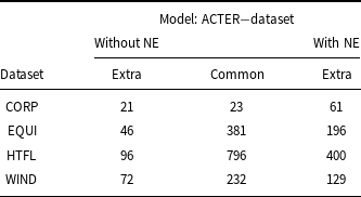
For ACTER data, we compare the results obtained by models trained on all annotated terms with models trained on data excluding NE annotations. The results for particular corpora are given in Table 15. Models trained with NE indicate NE phrases as terms, but our comparison concerns terms different from NE. The results show that the models trained with NE select more terms of other types (domain, general, out-of-domain); this relationship is noted by Rigouts Terryn (Reference Rigouts Terryn2021, p. 149). But similarly to the experiment described in Section 8.1, the models trained with NE stopped recognizing from 11% (EQUI, HTFL) to 49% (CORP) of correctly predicted terms by a corresponding model trained without NE.
Comparison of the lists of correctly predicted terms excluding named entities (NE) obtained by models tested with and without NE terms. The columns headed common give the number of correctly recognized terms by both models, and the columns headed extra give the number of extracted terms that are not common to both lists

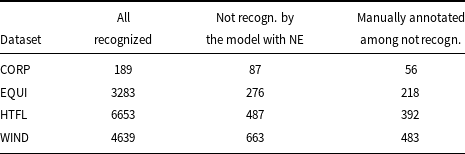
As in the previous section, we also checked the results of models without and with NE on the tokens level. We checked how many tokens recognized as a term component by the model without NE are not recognized by the model with NE. The results are given in Table 16. They show that adding NE to training data interferes with the recognition of other types of terms. If we don’t take into account the results for CORP data that are poor, from 7% to 14% of tokens recognized as term components by the model without NE are neglected by the model with NE. Around 80% of them are indicated as term components in GS.
The number of tokens recognized as a term component by the dataset model without named entities (NE) and not recognized by the model with NE. The columns headed all recognized give the number of tokens recognized as a term component by the models without NE. The next column gives the number of tokens recognized by the model without NE and not recognized as term components by the model with NE. The last column gives the number of tokens manually annotated as a term component within those in column 3
8.3 Context dependability
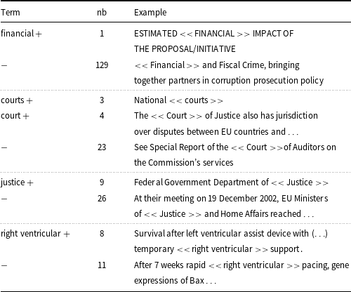
BERT-like models give answers depending on the context of the word (sequence) being analyzed. This is a positive feature, as the same expression can be or cannot be a term in a specific sentence. But on the other hand, specialized terms are introduced in very different ways, and we cannot always collect enough data to cover very many of them. The generality of the model is thus highly desirable. Unfortunately, when analyzing texts annotated with the help of our models, we can see that even if a specific term is recognized, it is only identified in some of the many contexts in which it is used. For example, in the CORP data, for the term financial, only one of nearly 130 examples is recognized. This is even more astonishing as, in the annotated files, there are about 20 types of multi-word terms which contain this word and none of them is recognized. This observation explains why the results for the short files are usually not good. It is not only the case that some terms occur only in the latter parts of the texts, but for some, only the latter examples are identified. The good results obtained for the short genotype data, confirm that there is a difference in vocabulary or style between this entry and the other Wikipedia articles we selected for testing. In Table 17, we show some examples of such positive and negative results. Somewhat surprisingly, the fact that the models sometimes recognize only very few (sometimes only one) occurrences of a given phrase in the text does not make the overall results worse when we compare the token labels with term-level evaluation. Correct recognition of some very frequent terms made the results very similar. We do not cite these results here,Footnote m as we are interested in the final list of terms, non-term occurrences.
Examples of terms from the ACTER corpus along with the number of their recognized (+) and unrecognized ( $-$
) occurrences in sentences
$-$
) occurrences in sentences

9. Conclusion
A lot of NLP tasks were successfully solved using contextual LLMs trained on data annotated with task-specific labels. The same solution was proposed for the terminology extraction task, and results better than previous ones were achieved. Nonetheless, they are not very high, as, for most experiments, F1 is around 0.6.
Our initial objective was to answer the question as to what types of terms are recognized by these models. We therefore performed a series of experiments, which unexpectedly showed that the method does not work well for all types of text. This prompted us to look for those text features for which the method works well. Our major findings are listed below.
First, using data from the most popular annotated set, ACTER, we found out that the results of the method vary a lot depending on the data used for training and testing. When the CORP set was used as the test set and NE were not treated as domain terms, the result was much worse than for the other sets. The model recognized only 5% of terms, while the results for the other ACTER corpora without NE are only slightly worse than those that include NE. The inclusion of NE in the set of terms skews the results, not only making the overall results higher but also changing which terms are recognized and which are not. We postulate that for new experiments, all NE should not be treated as terms and that the ATE should be tested on data with only domain-related NE annotated.Footnote n
Our analysis showed that the method recognizes only some (sometimes only very few) occurrences of a given term; it is thus natural that for short documents, results are typically worse than for the medium or long ones. However, the results for Wikipedia articles turned out to be unsatisfactory for only two of the three texts. As all these Wikipedia articles are short, it seems that the poor results for two of them cannot be attributed solely to their shortness.
Our experiments showed that poor results can correlate with the high frequency of tokens from the analyzed data in English texts. All corpora with poor results have the relatively high frequency calculated on data from TWC.Footnote o Another feature that seems to be important for the results of the method is the degree of overlap between the vocabulary of terms in the test data and the vocabulary of the training data. Table 11 shows that for the large analyzed corpora (ACTER and RD-TEC), incorrectly predicted terms have a higher percentage of overlapping vocabulary than correctly predicted terms. A high rate of vocabulary overlap may explain the poorer results for the WIND corpus. However, it seems that this factor may depend on the similarity of the testing domain and those used in training. The good results for WIKI-GEN might be partly due to the similar vocabulary of HTFL and WIKI-GEN.
We also show that the results obtained for a model trained on a bigger amount of data stopped recognizing quite a large percentage of terms (20%–30%) correctly identified by a model trained on a subset of this data. This property is not visible if we limit ourselves to only comparing the values of precision, recall, and F-measure. This proves that extending training data does not necessarily help in the case of ATE (the best F-measure for EQUI is obtained for the model trained on CORP + HTFL and not CORP + HTFL + WIND). Moreover, the experiment with a different random division of training data and learning on incremental data shows that the learning process is unstable. It seems to us that the instability comes from the fact that it’s difficult to find rules for recognizing a term based on the sentence itself. Each example points to individual unknown premises and is not generalizable, which means that different sets of learning examples lead to substantially different results.
The poor consistency of the results places a big question mark over the usefulness of the method in its current form, as it is not sufficient for the task. Independent of the language model used, further experiments to identify more text features which indicate that a specific phrase is a term are needed.
In answer to the question posed in the title, despite the weaknesses discussed in the paper, it should be stated that the transformer-based token classification ATE methods allow for the extraction of terms which are rare in general language and do not have to be frequent in an analyzed text. This is of considerable value for fields with specific vocabularies. Therefore, we should consider how to supplement the knowledge of models with information used by traditional methods, that is, frequency in the analyzed text and some knowledge of the domain of the text.
Competing interests
The authors declare none.


 Open access