

Introduction
Accurate biostratigraphy is essential to many areas of geology, paleontology, and evolutionary biology. The incompleteness of the fossil record, however, complicates the determination of stratigraphic ranges. Since the first or last occurrence of a fossil taxon is unlikely to be preserved in the fossil record, a taxon’s observed stratigraphic range invariably underestimates its true range. Building on the work of Shaw (Reference Shaw1964) and Paul (Reference Paul1982), Strauss and Sadler (Reference Strauss and Sadler1989) developed a statistical method to correct for this bias. However, their method requires the assumption that fossil recovery potential is uniform—that is, that fossil occurrences are equally likely to be found anywhere within the taxon’s true range. Much subsequent methodological and applied work has made the same assumption (Springer Reference Springer1990; Marshall Reference Marshall1990, Reference Marshall1995; Marshall and Ward Reference Marshall and Ward1996; Solow Reference Solow1996; Weiss and Marshall Reference Weiss and Marshall1999; Jin et al Reference Jin, Wang, Wang, Shang, Cao and Erwin2000; Solow and Smith Reference Solow and Smith2000; Ward et al. 2005; Solow et al. Reference Solow, Roberts and Robbirt2006; McInerny et al. Reference McInerny, Roberts, Davy and Cribb2006; Groves et al. 2007; Wang and Everson Reference Wang and Everson2007; Lindström and McLoughlin 2007; Wang et al. 2009; Angiolini et al. 2010; Wang et al. 2012; Tobin et al. 2012; Song et al. Reference Song, Wignall, Tong and Yin2013).
In practice, this assumption is rarely satisfied. For instance, if the taxon’s abundance and geographic range increase after its origination or decline prior to its extinction (Foote Reference Foote2007; Liow and Stenseth Reference Liow and Stenseth2007; Liow et al. Reference Liow, Skaug, Ergon and Schweder2010), and these factors affect recovery potential—as is almost certainly the case—then the assumption of uniform recovery potential would be violated. This assumption could also be violated for a number of other reasons—for instance, if the amount of available fossiliferous rock changes over time, if environmental conditions such as sea level change over time, if some parts of the true range are more difficult to sample than others, if some parts of the true range have been studied more intensely than others, or if there are facies changes or sequence boundaries in a fossiliferous section (Holland Reference Holland1995; Holland and Patzkowsky Reference Holland and Patzkowsky2002, Reference Holland and Patzkowsky2004, Reference Holland and Patzkowsky2007, Reference Holland and Patzkowsky2009; Scarponi and Kowalewski Reference Scarponi and Kowalewski2004; Patzkowsky and Holland Reference Patzkowsky and Holland2012). Under such common scenarios, methods assuming uniform recovery can give biased estimates, sometimes severely so (Holland Reference Holland2003; Solow Reference Solow2003; Wang et al. 2009; Rivadeneira et al Reference Rivadeneira, Hunt and Roy2009).
A number of methods have attempted to relax the assumption of uniform recovery potential. Two such methods, by Marshall (Reference Marshall1997) and Gingerich and Uhen (Reference Gingerich and Uhen1998), require a priori quantitative knowledge of recovery potential, but such information is often difficult to obtain. (Consider that even for as well-studied a group as the non-avian dinosaurs, there is widespread disagreement about whether they were increasing or decreasing in diversity before their ultimate extinction [Wang and Dodson Reference Wang and Dodson2006; Brusatte et al. Reference Brusatte, Butler, Barrett, Carrano, Evans, Lloyd, Mannion, Norell, Peppe, Upchurch and Williamson2015].) The method of Holland (Reference Holland2003) used ordination methods to estimate recovery potential, but his method is intended for larger datasets (typically at least “20–30 taxa and 50–60 samples”; Holland Reference Holland2003: p. 476) rather than for a single taxon. Other methods do not require a priori quantitative knowledge of recovery potential, but they may have other drawbacks. The method of Solow (Reference Solow1993) assumes only that recovery potential is exponentially decreasing at an unknown rate, but the author subsequently recommended against its use because its confidence intervals sometimes have no finite upper bound (Solow Reference Solow2005: p. 50). The method of Marshall (Reference Marshall1994) assumes that gaps between fossil finds are independent of stratigraphic position, but this assumption is often not satisfied and would be violated for a taxon with changing abundance or geographic range. The method of Solow (Reference Solow2003), originally proposed in a different context by Robson and Whitlock (Reference Robson and Whitlock1964), makes perhaps the fewest assumptions of any method, but it tends to yield wide intervals. Possibly the most promising method thus proposed is the Optimal Linear Estimation method of Roberts and Solow (Reference Solow2003), originally proposed in a different context by Cooke (Reference Cooke1980). This method is based on the fact that extreme order statistics follow a Weibull distribution under a broad range of conditions. In studies by Rivadeneira et al. (Reference Rivadeneira, Hunt and Roy2009), Collen et al. (Reference Collen, Purvis and Mace2010), and Clements et al. (Reference Clements, Worsfold, Warren, Collen, Clark, Blackburn and Petchey2013), this method was found to perform well as long as the sample size is not very small. Finally, a new Bayesian method was recently proposed by Alroy (Reference Alroy2014), but appeared too late for us to test in this paper.
The related topic of identifying extinctions has also been the subject of considerable research in the ecology and conservation biology literature (Solow Reference Solow1993, Reference Solow2005; McCarthy Reference McCarthy1998; Solow and Roberts Reference Solow and Roberts2003; McInerny et al. Reference McInerny, Roberts, Davy and Cribb2006; Roberts and Kitchener Reference Roberts and Kitchener2006; McPherson and Myers Reference McPherson and Myers2009; Rivadeneira et al. Reference Rivadeneira, Hunt and Roy2009; Vogel et al. Reference Vogel, Hosking, Elphick, Roberts and Reed2009; Collen et al. Reference Collen, Purvis and Mace2010; Jaric and Ebenhard Reference Jaric and Ebenhard2010; Akmentins et al. Reference Akmentins, Pereyra and Vaira2012; Clements et al. Reference Clements, Worsfold, Warren, Collen, Clark, Blackburn and Petchey2013; Thompson et al. Reference Thompson, Lee, Stone, McCarthy and Burgman2013; Clements et al. Reference Clements, Collen, Blackburn and Petchey2014; Caley and Berry Reference Caley and Barry2014). Work in these fields typically addresses the question of whether a taxon can be considered extinct based on sighting records. Here we focus on the paleontological topic of estimating the date of extinction of a taxon known to be extinct, but we note that our method may be applicable in ecological or conservation contexts as well.
In this paper, we propose a new method, the Adaptive Beta method, for estimating true stratigraphic ranges that does not assume that recovery potential is either uniform or known a priori. Instead, our method simultaneously estimates both the recovery potential and the true stratigraphic position (or time) of extinction from the positions of fossil occurrences of a single taxon. The method models recovery potential using a novel parametrization of the Beta probability density function, a flexible family of shapes that is able to model a variety of types of recovery potential. Because the method is derived using a Bayesian framework, it has the advantage of being able to explicitly account for prior information about either recovery potential or the position of the extinction if such information exists, but works even if such information does not exist. A further advantage is that the method produces Bayesian credible intervals that have a more natural interpretation than frequentist (classical) confidence intervals. We use simulations to assess the performance of our method compared to existing methods. We find that compared to existing methods, our method is most effective in achieving nominal coverage probabilities (e.g., having 90% credible intervals covering the true extinction 90% of the time) in a variety of situations. Finally, we demonstrate the method by applying it to a dataset of the Cambrian mollusc Anabarella.
Scales of Resolution
Recovery potential is the probability that a taxon will be known from the fossil record at a particular time. This function accounts for the combined probability of initial preservation, survival in the rock record until the present, and eventual discovery by paleontologists. Variation in recovery potential is necessarily dependent on the level of stratigraphic resolution being considered. At a sufficiently fine level of resolution, fluctuations in recovery potential are inevitable and may be substantial, due to facies control on fossil occurrences and sequence stratigraphic controls on facies changes in outcrops (Holland Reference Holland2000, Reference Holland2003; Holland and Patzkowsky Reference Holland and Patzkowsky2002; Patzkowsky and Holland Reference Patzkowsky and Holland2012). Over broader scales of resolution, recovery potential may change more gradually. For example, Holland (Reference Holland2003: Fig. 4) estimated recovery potentials for the trilobite Cryptolithus and the brachiopod Sowerbyella of the Upper Ordovician Kope Formation near Cincinnati. At the broadest scale of resolution, encompassing the entire 60 m of the Kope Formation in the dataset, it is apparent that there is a secular trend in which recovery potential decreases moving upwards through the section (this can be seen in Holland’s Figure 4 from the fact that fossil occurrences are more common lower in the section and become much less common as we move upwards). Within some 20-meter sedimentary cycles, however, there is little secular trend in recovery potential of either taxon. At this intermediate scale of resolution, it may be reasonable to consider the recovery function to be approximately uniform. At a finer level of resolution, however, substantial high-frequency variation corresponding to meter-scale sedimentary cycles is present.
Holland (Reference Holland2003) was able to estimate recovery potential at a very high resolution using a large dataset with 46 taxa and 1337 beds. By pooling the information from multiple taxa, he was able to apply ordination methods such as detrended correspondence analysis. In contrast, we assume the presence of only a single taxon, typically known from a few to a couple of dozen locations in the stratigraphic section. Clearly, with datasets of this size, it will be impossible to estimate recovery potential at the fine level of resolution achieved by Holland (Reference Holland2003). Rather, we aim to estimate recovery potential at a coarser level, similar to that of the 20-meter cycles shown in Figure 4 of Holland (Reference Holland2003). That is, we aim to estimate the gradual changes in recovery potential occurring over a series of beds, rather than individual bed-by-bed changes in recovery potential.
Modeling the Recovery Function: The Reflected Beta Distribution
In this section, we describe the Reflected Beta distribution, which we use to model the recovery function. Suppose the true range of a taxon spans the interval [0, θ], where 0 represents the point relative to which measurements are being made (e.g., the base of the stratigraphic section), and θ represents the position corresponding to the extinction of the taxon. The goal is to estimate θ from only the stratigraphic positions of fossil occurrences, x 1… x n, typically in units of meters above the base of the stratigraphic section or in units of time. (We will henceforth refer only to stratigraphic position for the sake of simplicity.) We denote the vector x 1… x n by x, and we assume without loss of generality that x 1 < x 2 < … < x n, with x 1 being the lowest (oldest) and xn the highest (youngest) fossil occurrence. Note that 0 is defined here so that the taxon is extant at that point. If there is no natural candidate for a baseline level corresponding to 0, we can set the position of the first (oldest) occurrence equal to 0 and rescale the other occurrences accordingly. In that case, we omit the first occurrence from further calculations and reduce the sample size by one, as recommended by Solow (Reference Solow2005).
Let f(x) denote the fossil recovery function, which describes fossil recovery potential as a function of stratigraphic position. Depending on the context, we will often write f(x) as f(x|parameters) to explicitly show the dependence of f(x) on one or more parameters. We assume f(x) is unknown.
To model f(x), we introduce the Reflected Beta distribution. This distribution is a novel variant of the Beta (α, β) distribution, a standard distribution whose probability density function (pdf) is given by the equation:
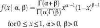 $$f\left( {x{\rm\, \mid \ralpha },\,{\rm \rbeta }} \right)= {{{\rm \Gamma }\left( {{\rm \ralpha{\plus}\rbeta}} \right)} \over {{\rm \Gamma }({\ralpha})\:{\rm \Gamma }({\rbeta})}}x^{{{\ralpha }\;-{\rm 1} }} ({\rm 1}{\minus}x)^{{{\rm \rbeta }-{\rm 1}}} \quad {\rm for}\,0\,\leq \,x\leq {\rm 1},\,{\rm \ralpha }\,\gt\, 0,\,{\rm \rbeta }\,\gt\, 0.$$
Here x denotes stratigraphic position scaled to the interval [0, 1], α and β are parameters governing the shape of the distribution, and Γ() denotes the gamma function, given by 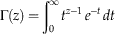 $\Gamma (z)=\mathop{\int}\nolimits_0^\infty {t^{{z{\minus}1}} \,e^{{{\minus}t}} } \,dt$
. Note that the term in the pdf involving gamma functions is simply a normalizing constant that ensures that the pdf will integrate to 1, as all pdfs must do. The Beta distribution is useful in modeling a range of phenomena because it can take on a variety of shapes, including bell-shaped, right- or left-skewed, increasing or decreasing, or flat.
$\Gamma (z)=\mathop{\int}\nolimits_0^\infty {t^{{z{\minus}1}} \,e^{{{\minus}t}} } \,dt$
. Note that the term in the pdf involving gamma functions is simply a normalizing constant that ensures that the pdf will integrate to 1, as all pdfs must do. The Beta distribution is useful in modeling a range of phenomena because it can take on a variety of shapes, including bell-shaped, right- or left-skewed, increasing or decreasing, or flat.
The Reflected Beta model
We modify the standard Beta distribution in two ways. First, we want the recovery function to be a function of a single parameter, which we call λ, rather than the two parameters α and β. It is convenient to parametrize this variant of a Beta distribution so that λ < 0 corresponds to decreasing recovery potential, λ=0 to uniform recovery potential, and λ>0 to increasing recovery potential. To satisfy this property, we define the Standard Reflected Beta distribution as follows:
 $$\kern-6pt f\left( {x{\rm \,\mid }\, \rlambda } \right)\,\sim\,{\rm Beta}({\rm 1},\,{\rm 1}{\minus}{\rm \rlambda })\quad {\rm if}\,{\rm \rlambda }\leq 0,\,0\leq x\leq {\rm 1},$$
 $$\kern-4pt f\left( {x{\rm \, \mid \rlambda }}\, \right)\,\sim\,{\rm Beta}\left( {{\rm 1}{\plus}{\rm \rlambda },\,{\rm 1}} \right) \,{\rm if}\ {\rm \rlambda }\,\gt\, 0,\,0\,\leq\, x\,\leq \,{\rm 1}.$$
The pdf of the Standard Reflected Beta distribution can be found by substituting the parameters from equations (2) and (3) into equation (1) above, which gives us the following pdf:
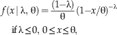
 $$f\left( {x\, {\rm \mid \rlambda }} \right)=({\rm 1}{\minus}{\rm \rlambda })\,({\rm 1}{\minus}x)^{{-{\rm \rlambda } }} \; {\rm if}\,{\rm \rlambda }\leq 0,\,0\leq x\leq {\rm 1},$$
 $$f\left( {x\, {\rm \mid \rlambda }} \right)=\left( {{\rm 1}{\plus}{\rm \rlambda }} \right)x^{{\rm \rlambda }} \,\quad {\rm if}\,{\rm \rlambda }\,\gt\, 0,\,0\,\leq \,x\,\leq \,{\rm 1}.$$
In equations (2)–(5), x denotes stratigraphic position scaled to the interval [0, 1].
The second modification is that we want the recovery function to be defined over the taxon’s true range, corresponding to the interval [0, θ], rather than just the unit interval [0, 1]. Using standard techniques of mathematical statistics, it is straightforward to rescale the Standard Reflected Beta pdf so that it is defined over the interval [0, θ], which gives us the following Reflected Beta pdf:
 $$f\left( {x\, {\rm \mid \rlambda },\,{\rm \rtheta }} \right)= {{\left( {1{\minus}\rlambda} \right)} \over {\rm \rtheta}}({\rm 1}{\minus}x/{\rm \rtheta })^{{-{\rm \rlambda }}} \,\quad {\rm if}\,{\rm \rlambda }\leq 0,\,0\leq x\leq {\rm \rtheta }, $$
 $$f\left( {x{\rm \,\mid \rlambda },\,{\rm \rtheta }} \right)={{\left( {1{\plus}\rlambda} \right)} \over {\rm \rtheta}} \left( {x/{\rm \rtheta }} \right)^{{\rm \rlambda }} \quad {\rm if}\,{\rm \rlambda }\,\gt \,0,\,0\leq x\leq {\rm \rtheta }. $$
In equations (6)–(7), x now denotes the actual stratigraphic position (i.e., in raw units such as meters or feet rather than scaled to the interval [0, 1]). Note that because we have now introduced the additional parameter θ, we write the pdf as f(x|λ,θ) instead of just f(x|λ) as in equations (2)–(5). Henceforth, when we refer to the Reflected Beta pdf, we mean this rescaled version given by equations (6)–(7).
Examples of Reflected Beta pdfs are shown in Figure 1, with five particular examples used in our simulations shown in Figure 2. The pdfs are always monotonic and often resemble exponential functions. As λ varies from negative to zero to positive values, f(x) varies from decreasing to uniform to increasing recovery potential as we approach the true extinction. We are thus able to model recovery functions with a variety of shapes, indexed only by the single parameter λ. We emphasize that it is not necessary to specify in advance whether f(x) is decreasing, uniform, or increasing; rather, the value of λ (and thus the shape of the recovery function) will be estimated automatically from the data.

Figure 1 Examples of the Reflected Beta distribution for values of λ from –5 to +5 in increments of 0.2. The distribution is able to model a variety of shapes.
Figure 2 Examples of the Reflected Beta distribution for λ = −2, −1, 0, +1, and +2. The distribution is able to model a range of decreasing, uniform, and increasing recovery potentials. These five values of λ are used in our simulation study.
A Bayesian Model
In this section we describe a Bayesian model that uses the Reflected Beta model for the recovery function, together with information from observed fossil occurrences, to derive a credible interval for the true extinction θ. A credible interval is the Bayesian analogue to a frequentist confidence interval. Below we discuss advantages of credible intervals over standard confidence intervals; see also Wang (Reference Wang2010) for a more general discussion of the advantages and disadvantages of the Bayesian approach. To calculate the credible interval, we begin with a prior distribution on the parameters. We then show how to use the observed data to update this prior distribution. We thus arrive at the posterior distribution, which quantifies our knowledge of the parameters in light of the observed data.
Prior distribution
A prior distribution quantifies our knowledge of (or conversely, our uncertainty about) the values of the parameters prior to observing any data. Here we have two parameters, θ (representing the true position or time of the extinction) and λ (governing the shape of the Reflected Beta recovery function). When one does not wish to specify any a priori knowledge about the parameters, one can use a uniform (flat) prior, under which all possible parameter values are given equal weight. However, this does not seem to be a reasonable choice in our case. Surely it is not the case that the true extinction of the non-avian dinosaurs is equally likely to have occurred at 66 Ma as, say, last Tuesday. Similarly, not all values of λ are equally plausible. Therefore, we use informative (non-uniform) prior distributions for both θ and λ.
For θ, we use a prior of 1/θ, giving more weight to smaller values of θ. In other words, larger values of θ, which indicate larger gaps between the last fossil occurrence and the actual time of extinction, are deemed to be less probable than smaller gaps. This prior results in values closer to and above x n (the taxon’s highest occurrence) having higher probability; values below x n will turn out to have zero posterior probability when we multiply the prior by the likelihood function described below.
For λ, we use a Normal prior with mean=0 and standard deviation=2. Because we want our method to work for a variety of datasets, we do not wish to express an a priori preference for either a decreasing or increasing recovery function, and the Normal (0, 2) prior reflects this preference because it is symmetric about zero. The Normal (0, 2) prior also gives higher weight to values of λ closer to zero (corresponding to flatter recovery potentials), and the choice of 2 for the standard deviation puts 95% of the prior probability between −4 and +4. This choice of prior avoids over-weighting extreme values of λ, which would lead to unnecessarily wide intervals.
We assume that θ and λ are independent, so that their joint prior distribution, denoted by π(θ, λ), is equal to the product of the individual prior distributions. Hence the prior distribution π(θ, λ) is given by
 $${\rm \pi }\left( {{\rm \rtheta },\,{\rm \rlambda }} \right)= {1 \over {2{\rm \rtheta}\sqrt {2{\rm \pi }} }}e^{{-{\rm \rlambda }^{{\rm 2}} /{\rm 8}}} \,\quad {\rm for}\,\,{\rm \rtheta }\,\gt\, 0,{\minus}\infty\,\lt\, {\rm \rlambda }\,\lt\, \infty$$
Figure 3A shows the prior distribution as a three-dimensional surface over the plane whose axes are values of θ and λ. The highest values of the surface, and thus the region of highest prior probability, are shown in lighter shading. One can see that the prior is highest for values of θ that are relatively small and λ values that are relatively close to zero. The prior falls off quickly for extreme values of λ but more slowly for large θ values.
Figure 3 Prior distribution, likelihood surface, and posterior distribution of λ (parameter describing recovery potential) and θ (parameter representing the true extinction). The dataset is an artificial one randomly generated from a recovery function with λ=−1 and has six fossil occurrences at 3.9, 14.5, 15.3, 27.0, 37.2, and 62.1 meters; the extinction was set to θ=100 meters. Light shading indicates higher values; dark shading indicates lower values. A, The prior gives higher weights to values of λ near 0 and smaller values of θ. B, The likelihood surface has a broad peak over a region of the parameter space running from the middle left to the bottom right of the panel, demonstrating that the data are consistent with either an increasing recovery function and small gap between the highest fossil occurrence and the true extinction, or a decreasing recovery function and a large gap. C, The posterior combines information from both the prior and the likelihood (giving more weight to the likelihood as the sample size increases), which constrains the most probable values of λ and θ.
Our choice of prior is intended to be reasonable for a broad range of datasets. Of course, if there is prior information for a particular locality, then our prior distribution can be replaced with one that is more appropriate. In fact, the ability to incorporate such prior information is one of the advantages of the Bayesian approach. We also tried a variety of other prior distributions, and we found that the results were moderately robust when using similarly shaped priors (i.e., decreasing as a function of θ and symmetric as a function of λ). We also tried a uniform prior, which did not work well. As described above, a uniform prior does not conform to common sense knowledge about θ and λ, and given the small sample sizes typical in this setting, the likelihood function is too diffuse to be sufficiently informative with a uniform prior.
Note that this prior is an example of an improper prior—i.e., it does not integrate to one and thus is not a proper probability distribution—because the integral of 1/θ diverges. However, this is not a problem, as the posterior distribution turns out to be proper as long as we have at least one observed fossil occurrence.
It is arguably the case that θ and λ should not be treated as independent. We have chosen to proceed under this assumption for now, but how to model the relationship between the two parameters remains an area of further investigation.
Likelihood
The likelihood function quantifies the information about the parameters that is contained in the data. Denoted by L(θ,λ|x), the likelihood is numerically equal to the joint probability (pdf) of the fossil occurrences given the parameters, P(x 1…x n|θ,λ), but the likelihood is viewed as a function of the parameters, rather than as a function of the fossil occurrences. In our case, it is straightforward to calculate the value of the joint pdf for any specified value of θ and λ. For a single fossil occurrence xi, the joint pdf is given by the value of the recovery function evaluated at xi, namely f(xi|λ,θ) as given by equations (6)–(7). For the entire set of fossil occurrences, which are assumed to be independent, the joint probability is the product of these individual probabilities. Thus the likelihood L(θ, λ|x) is equal to
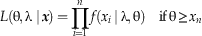 $$L\left( {{\rm \rtheta },{\rm \rlambda \mid \,}\mib x} \right){\rm }= \prod\limits_{i=1}^n {f\left( {x_{{i }} \,{\rm \mid \rlambda },{\rm \rtheta }} \right)} \quad {\rm if}\,{\rm \rtheta }\geq x_{n} $$
Figure 3B shows the likelihood surface as a function of θ and λ, using a small artificial dataset of six occurrences, randomly generated from a recovery function having λ=−1 and θ=100. The most likely values of θ and λ lie along a light-colored band in which the two parameters are inversely correlated. This reflects the fact that for a given dataset, larger values of θ (and therefore a larger gap after the highest occurrence) are likely when lambda is strongly negative, and smaller values of θ (corresponding to a smaller gap after the highest occurrence) are likely when λ is strongly positive.
Posterior distribution
The goal of a Bayesian analysis is to compute the posterior distribution, which quantifies our knowledge about the value of θ and λ after (i.e., posterior to) observing the fossil occurrences x. According to Bayes Theorem, the posterior distribution is proportional to the product of the prior distribution and the joint likelihood. (Because we are concerned with the relative probability of a parameter value compared to other parameter values, rather than its probability in an absolute sense, it is sufficient for our purposes to determine the proportional value of the posterior distribution.) Thus, the joint posterior of θ and λ, denoted by π(θ, λ|x), is calculated as follows:
 $$\eqalignno{ & {\rm \pi }\left( {{\rm \rtheta ,}\,{\rm \rlambda \mid }\,\mib x} \right)\propto{\rm \pi }\left( {{\rm \rtheta ,}\,{\rm \rlambda }} \right)\,L\left( {{\rm \rtheta },\,{\rm \rlambda }\mid \mib x} \right) \cr & = {1 \over {2{\rm \rtheta}\sqrt {2{\rm \pi }} }}e^{{-{\rm \rlambda }^{{\rm 2}} /{\rm 8}}} \prod\limits_{i=1}^n { f\left( {x_{i} \mid {\rm \rlambda },\,{\rm \rtheta }} \right)} \,\quad {\rm if}\,{\rm \rtheta }\geq x_{n} $$
This joint posterior distribution is shown in Figure 3C, which can be thought of as the product of multiplying each pixel in Figure 3A by the corresponding pixel in Figure 3B. Here the highest values are ones that have high prior values and high likelihood values. Within the light-colored band having high likelihood, the upper left (white) region has the highest posterior probability, because that portion also has a high prior probability. By contrast, the lower right portion has a low prior probability, which reduces its posterior probability. Thus the most probable combination of parameter values for this dataset has θ between approximately 62 and 100, and λ between approximately 0 and −2. Note that the posterior (Fig. 3C) resembles the likelihood (Fig. 3B) more closely than it does the prior (Fig. 3A), meaning that the posterior is determined more strongly by the observed data than by our prior belief, which is appropriate, although the prior does exert some influence in ruling out implausible regions of the posterior.
Marginal posterior distribution of θ
In our situation, we are primarily concerned with estimating θ, the position of the extinction. Our goal is therefore to find the posterior distribution of θ alone, with λ considered to be a nuisance parameter (one that is not of primary interest). To find this posterior distribution of θ alone, denoted by π(θ|x) and also referred to as the marginal posterior of θ, we can integrate out λ by integrating over all possible values of λ:
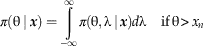 $${\rm \pi }( { \rtheta }\mid }{\mib x}} \right)=\mathop{\int}\limits_{{\minus}\infty}^\infty { {\rm \pi }\left( {{\rm \rtheta },{\rm \rlambda \mid }\, {\mib x} \right)d{\rm \rlambda } } \,\quad {\rm if}\,{\rm \rtheta }\, \gt \, x_{n} $$
This integration has a visual analogue. Consider the joint posterior of θ and λ in Figure 4A (this is the same as in Figure 3C, repeated for convenience). This surface gives the (posterior) probability of θ and λ, whereas what we want is the probability of θ alone, regardless of λ. For example, rounding to the nearest whole value of θ, we want the probability that θ=100 regardless of λ, the probability that θ=101 regardless of λ, the probability that θ=102 regardless of λ, and so on. Consider (e.g.) the probability that θ=101 regardless of λ: this is equal to the probability that θ=101 when λ=0, plus the probability that θ=101 when λ=0.1 (rounding to the nearest tenth), plus the probability that θ=101 when λ=0.2, and so on. If we sum the probabilities of θ=101 for all values of λ (including negative values), we will arrive at the overall (marginal) probability of θ=101, regardless of λ. Visually, this simply corresponds to summing the probabilities in each column of Figure 4A—in other words, summing the heights of the three-dimensional surface above each strip running parallel to the λ axis. Analytically, this is equivalent to integrating the surface over the λ axis—the integral in equation (11). Often this integral cannot be solved analytically, but in our case it can be calculated numerically.
Figure 4 Joint posterior distribution of λ (recovery function parameter) and θ (true extinction), and marginal posterior distributions of λ and θ. The dataset is the same as in Figure 3, with six randomly generated fossil occurrences at 3.9, 14.5, 15.3, 27.0, 37.2, and 62.1 meters; the extinction was set to θ=100 meters. A, The joint posterior is the same as in Figure 3C and is repeated here for convenience. B, The marginal posterior for θ is found by integrating over all values of λ, which corresponds graphically to summing vertically down the columns of the joint posterior in 4A. C, The marginal posterior of λ is found by integrating over all values of θ, which corresponds graphically to summing horizontally across the rows of the joint posterior in 4A. The posterior mean is used as a point estimate for λ, and the posterior median for θ due to skewness in the posterior distribution for the latter. Point estimates for θ and λ were 98.5 meters (asterisk in 4B) and −1.7 (diamond in 4C), respectively. In other words, there is a gap of (100–62.1)=37.9 meters between the highest occurrence and the true extinction, and based only on these six occurrences, the method is able to estimate a gap of (98.5–62.1)=36.4 meters. The upper endpoint of the confidence interval is 177.8 meters (shaded region of 4B).
The resulting marginal posterior distribution, π(θ|x), quantifies all of our knowledge about θ in light of the observed data (Fig. 4B). Once we have arrived at this distribution, it is straightforward to calculate quantities of interest. For instance, for a point estimate of θ, we might use the posterior median (Fig. 4B, asterisk). For a 100(1 − α)% credible interval for θ, we take the range from the highest fossil occurrence to the 100(1 − α)th percentile of π(θ|x). For example, a 90% credible interval (corresponding to α =.10) is the range up to the 90th percentile of π(θ|x) (Fig. 4B, gray shaded region). We call this method the Adaptive Beta method, as the method is designed to adapt to unknown recovery functions rather than requiring that the recovery function be known and specified.
Note that our method is scale-invariant. That is, the results do not depend on whether the units of measurement are, e.g., in meters or feet.
Marginal posterior distribution of λ
Although not of primary interest here, the marginal posterior distribution of λ alone can be determined similarly. To find π(λ|x), we integrate out θ by integrating over all possible values of θ:
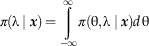 $${\rm \pi } {{ \left(\rlambda }\mid {\mib x} \right){\rm }=\mathop{\int}\limits_{{\minus}\infty}^\infty {\rm \pi }\left( {{\rm \rtheta ,}\,{ \rlambda}\mid {\mib x}} \right)d\,{\rm \rtheta }$$
This corresponds to summing the probabilities across each row of Figure 4A—in other words, summing the heights of the three-dimensional surface above each strip running parallel to the θ axis. The resulting marginal posterior distribution quantifies our knowledge of λ in light of the observed data, indicating the shape of the recovery function (e.g., decreasing, flat, or increasing).
Simulation Results
To verify that the method works as intended, we ran simulations using artificial datasets. We arbitrarily set θ equal to 100 and then randomly simulated datasets with fossil occurrences falling between 0 and θ, following five different recovery functions: Reflected Beta distributions having λ=−2, −1, 0, +1, and +2. Sample sizes ranged from 5 to 25 fossil occurrences. For each dataset, we calculated a 90% confidence interval or credible interval and a point estimate for θ using five methods:
1. The method of Strauss and Sadler (Reference Strauss and Sadler1989), here denoted SS89.
2. The sighting-rate-based method of McInerny et al. (Reference McInerny, Roberts, Davy and Cribb2006), denoted M06.
3. The last-gap method of Solow (Reference Solow2003), denoted S03
4. The Optimal Linear Estimation-based method of Roberts and Solow (Reference Solow2003), denoted RS03, also known as the Weibull method. Results are shown using k=10 as in Roberts and Solow (Reference Solow2003) and Rivadeneira et al. (Reference Rivadeneira, Hunt and Roy2009). We also tried k=n as recommended by Clements et al. (Reference Clements, Worsfold, Warren, Collen, Clark, Blackburn and Petchey2013), but found k=10 worked slightly better.
5. The new Adaptive Beta method presented in this paper, denoted ABM.
Methods SS89 and M06 assume uniform recovery and were not expected to work well for non-uniform recovery functions, but are included as a baseline for comparison. The other three methods do not make any assumptions about the recovery function, and are thus directly comparable. For each method, we recorded the following information: (1) how often the intervals covered the true value of θ=100 (the empirical coverage probability); (2) the widths of the intervals, indicating how precisely the method is able to pinpoint the true extinction; and (3) the point estimates for θ, the best guess for the true extinction. For the Adaptive Beta method, we also recorded the point estimate for λ, the parameter describing the shape of the recovery function.
Our simulations differ from other studies that have compared the performance of various confidence interval methods (Rivadeneira 2009; Bradshaw et al. 2012). First, we use smaller sample sizes, ranging from five to 25 fossil occurrences per taxon, which are typical in paleontology. Rivadeneira (2009) appeared in the ecological literature and uses sample sizes from 20 to 120, which are more typical of datasets in that field. Bradshaw et al. (2012) focuses on Pleistocene and archaeological examples, and uses sample sizes of 50. Because we are using substantially smaller datasets, we are testing the methods under more difficult conditions. Second, we test datasets generated from a different set of recovery functions (although our choices overlap with those used by the other papers). Third, we assume the locations of fossil occurrences, x 1…x n, are known without error, whereas Bradshaw et al. (2012) account for radiometric dating error in these values. Their choice is appropriate because their paper focuses on datasets of Quaternary age that are typically dated using radiometric methods (e.g., 14C) with known margin of error. By contrast, we assume our method will be applied to paleontological datasets consisting of stratigraphic positions, for which measurement error is negligible compared to the effects of incomplete fossil preservation. Fourth, we use a different (although overlapping) set of criteria to judge the accuracy and precision of the methods being tested.
Main simulation results
We found that SS89 and M06 performed similarly and had poor coverage probabilities when the recovery function was decreasing (Fig. 5; see Supplemental Information (http://dx.doi.org/10.5061/dryad.224hj) for a version of this figure accessible to readers with color-deficient vision). For recovery functions with λ=−2, the nominal 90% intervals of SS89 and M06 correctly covered the true value of θ in less than 25% of datasets, and in fact performed worse as the sample size increased. Methods S03, RS03, and ABM, which do not assume uniform recovery, performed better under these conditions. For λ=−2, all three methods covered the true value of θ in at least 50% of datasets. However, only ABM was able to achieve a coverage probability close to the nominal 90% level, covering the true value of θ in at least 80% of datasets except for the smallest sample sizes. None of the other methods achieved 80% coverage at any sample size when λ=−2. Method S03 covered the true value of θ in just under 75% of datasets regardless of sample size, and RS03 in just under 60% of datasets except at small sample sizes.
Figure 5 Results from simulations comparing the methods of Strauss and Sadler Reference Strauss and Sadler1989 (black), McInerny et al. Reference McInerny, Roberts, Davy and Cribb2006 (orange), Solow Reference Solow2003 (blue), Roberts and Solow Reference Solow2003 (green), and the Adaptive Beta Method (red). Simulations were run using sample sizes from 5 to 25 occurrences, randomly generated from reflected Beta distributions with shape parameter λ varying from −2 to +2. For each value of λ and each sample size, 10,000 simulated datasets were randomly chosen, so the total number of simulated datasets in the figure is (5)(21)(10,000)=1,050,000. The same datasets were used for all five methods. Top row shows the shape of the recovery potential function for each column. Second row shows the empirical coverage probability (the percent of intervals that correctly covered the true extinction) for each method; gray lines denote the nominal coverage probability of 90%. Third row shows the mean width of the intervals for each method. Fourth row shows the estimates of θ, the true extinction time (here set to θ=100, denoted by the gray lines) for each method. Bottom row shows the estimates of λ for the Adaptive Beta method; gray lines denote the true value of λ. A version of this figure for those with color-deficient vision is given in the Supplemental Information.
For λ=−2, the mean widths of the confidence intervals found by SS89 and M06 were the smallest, but these methods (which assume uniform recovery) do not give sufficiently wide intervals to account for the uncertainty introduced by non-uniform recovery functions. The intervals produced by S03 were much wider—a drawback acknowledged by Solow (Reference Solow2005: p. 51)—possibly to the extent that the intervals would no longer be practically useful. The intervals of RS03 and ABM were intermediate in width. For λ=−2, none of the methods was able to give accurate point estimates of θ. Method ABM worked best, approaching 10% relative error for sample sizes larger than 15. The other methods were typically too low by 20–40%.
For recovery functions with λ=−1, the methods gave similar results to the λ=−2 case but were somewhat more successful. Method ABM was the only one to achieve a coverage probability of 90%. Method S03 covered the true value of θ in approximately 80% of datasets, RS03 in 70–80%, and SS89 and M06 less than 50%. As with λ=−1, S03 had very wide intervals, ABM slightly less so, and RS03 even less. Method ABM gave the most successful point estimates for θ, usually falling within about 0–5% relative error. Method RS03 was next best at around 5–8% error, while the other methods rarely came within 10% of the correct value.
For the uniform recovery case of λ=0, not surprisingly, method SS89 (which assumes uniform recovery) worked best. All methods covered the true value of θ at least 90% of the time, except M06, which was near 85%. Methods SS89 and M06 had the narrowest intervals. All methods gave point estimates accurate within approximately 10% except ABM at small sample sizes, with SS89 being unbiased, as would be expected from statistical theory (Strauss and Sadler Reference Strauss and Sadler1989; Wang et al. 2009). Method ABM was biased upwards and RS03 slightly less so, whereas M06 was biased slightly downwards.
The cases in which fossil recovery is increasing (λ=+1 and +2) are in some sense the “easy” cases because fossil occurrences become more common as we approach θ. All five methods were able to achieve the nominal 90% coverage probability. Interval widths were similar for most of the methods, with ABM giving the narrowest intervals (except at small sample sizes for λ=+1) because it accounts for the fact that the gap between the last occurrence and θ is smaller when recovery potential is increasing. Point estimates were accurate within approximately 10%; ABM and S03 were closest to unbiased, whereas the other three methods were biased slightly upwards for smaller sample sizes.
Estimating λ
Although our primary interest is in estimating θ, the true time of extinction, the ABM also gives an estimate of the shape parameter of the Reflected Beta distribution (Fig. 5, bottom row). The estimated λ was close to the actual value for λ>0, but was less successful for λ ≤ 0. The reason for this behavior is not clear. The ABM underestimated λ when λ=0 or −1, which was probably responsible for its upward bias in estimating θ in those cases. Conversely, the ABM overestimated λ when λ=−2, which was probably responsible for its downward bias in estimating θ in that case.
Additional simulation results
In the simulations discussed so far, we generated datasets from a fossil recovery function that in fact followed a Reflected Beta distribution, meaning that the model assumed by the ABM was correct for these datasets. This gives the ABM an advantage relative to the other methods, so we also simulated data from three additional recovery functions that do not follow a Reflected Beta distribution: logistic (sigmoidal), exponential, and stepwise (Fig. 6; see the Supplemental Information (http://dx.doi.org/10.5061/dryad.224hj) for a version of this figure accessible to readers with color-deficient vision). Note that the stepwise recovery function has the property that it drops abruptly to zero at position θ, unlike the decreasing Reflected Beta recovery functions with λ=−2 and −1, which decline gradually to zero at position θ. The logistic and exponential recovery functions also have an abrupt drop to zero, although in both of these cases the drop is so small that for all intents and purposes they can be considered to be gradually declining to zero. A recovery function with an abrupt drop may be more appropriate when an extinction is sudden (e.g., in a mass extinction caused by a bolide impact), whereas a gradually declining recovery function may be more plausible for a taxon going extinct gradually.
Figure 6 Results from simulations comparing the methods of Strauss and Sadler Reference Strauss and Sadler1989 (black), McInerny et al. Reference McInerny, Roberts, Davy and Cribb2006 (orange), Solow Reference Solow2003 (blue), Roberts and Solow Reference Solow2003 (green), and the Adaptive Beta Method (red) on datasets randomly generated from recovery functions other than the Beta distribution. Recovery functions used were logistic (left column), exponential (middle column), and stepwise (right column). See Figure 5 caption for details. For each recovery function and each sample size, 10,000 simulated datasets were randomly chosen, so the total number of simulated datasets in the figure is (3)(21)(10,000)=630,000. A version of this figure for those with color-deficient vision is given in the Supplemental Information.
For all three of these additional recovery functions, the results were similar. Method ABM was the only one to achieve a coverage probability of 90%. Method S03 covered the true value of θ in approximately 83–86.5% of datasets, RS03 in approximately 80%, and SS89 and M06 less than 60%. Methods S03 and ABM had very wide intervals; the intervals of method RS03 were narrower but still quite wide. Method RS03 had the most successful point estimates for θ, falling within about 3% error for sample sizes greater than 7. None of the other methods was able to give accurate point estimates for θ, with ABM generally overestimating θ and the other three methods underestimating θ.
An Illustrative Example: The Origination of Anabarella
We demonstrate the use of the Adaptive Beta method by estimating the time of origination of the Cambrian mollusc Anabarella. Although we have described the method thus far in terms of estimating extinction, here we use the method for origination, which is mathematically equivalent. We apply the Adaptive Beta method to a dataset of 19 occurrences of Anabarella compiled from several Cambrian localities in Siberia and Mongolia (Maloof et al. Reference Maloof, Porter, Moore, Dudas, Bowring, Higgins, Fike and Eddy2010). These occurrences were correlated and dated using carbon isotope curves and range in age from 522.20 Ma to 533.07 Ma (Fig. 7A). Because there is no point that intrinsically corresponds to a baseline time of zero, we follow the recommendation of Solow (Reference Solow2005) in taking the age of the youngest occurrence as the zero point and reducing the sample size by one.
Figure 7 A, Histogram of ages of 19 fossil occurrences of the Cambrian mollusc Anabarella from Siberia and Mongolia (Maloof et al. Reference Maloof, Porter, Moore, Dudas, Bowring, Higgins, Fike and Eddy2010). Histogram bars denote the number of occurrences found in each 2 million year bin. Curve denotes the Reflected Beta recovery function as estimated by the Adaptive Beta method, with the estimated origination at θ=535.1 Ma (asterisk). Vertical ticks at the bottom of histogram bars denote ages of individual fossil occurrences. The youngest occurrence at 522.20 Ma was taken as the baseline or zero point and excluded from the calculations, following the recommendation of Solow (Reference Solow2005). B, Posterior distribution of λ, with the posterior mean being λ=−0.95 (diamond). C, Posterior distribution of θ, with the posterior median being θ=535.1 Ma (asterisk). The 90% credible interval given by the Adaptive Beta method extends to 542.4 Ma (gray shaded region).
The method of Strauss and Sadler (Reference Strauss and Sadler1989), which assumes uniform preservation, estimates an origination date of 533.67 Ma, with a 90% confidence interval extending to 534.55 Ma. However, the data suggest that recovery potential may not be uniform and instead may decrease towards the time of origination, as there are fewer older than younger occurrences, and the two oldest occurrences are separated by a substantial gap. Moreover, as recovery potential is likely to depend on abundance and geographic range, it seems reasonable that recovery potential would be lower near the time of origination, when populations would presumably be smaller and less widely distributed. The Adaptive Beta method is able to detect this decrease in recovery potential, as it gives a point estimate for λ equal to −0.95, indicating an approximately linearly decreasing recovery function (Fig. 7B). The point estimate for θ, the time of origination, is 535.1 Ma, and the 90% credible interval extends to 542.4 Ma (Fig. 7C). Both the point estimate and interval estimate are earlier than the corresponding estimates from the Strauss and Sadler (Reference Strauss and Sadler1989) method, due to the ABM accounting for the decreasing probability of finding fossils further back in time. In fact, the endpoint of the 90% credible interval extends beyond the base of the Cambrian (given as 541.0 ±1.0 Ma in Cohen et al. Reference Cohen, Finney, Gibbard and Fan2013). To estimate the probability that Anabarella originated before the Cambrian, we note that 541.0 Ma would be the endpoint of an 87% credible interval—i.e., 87% of the posterior distribution falls after 541.0 Ma and 13% before. Thus there is a 13% probability that the origination of Anabarella predated the Cambrian. This kind of probability interpretation is often attached to frequentist confidence intervals, but incorrectly so, as noted by Alroy (Reference Alroy2014). However, a Bayesian credible interval can correctly be interpreted in this natural way—an advantage of the Bayesian approach.
Code for the ABM was written using R version 3.1.0 (http://www.r-project.org) and is given in the Supplementary Information (http://dx.doi.org/10.5061/dryad.224hj). The example above took 0.4 seconds to run on a 2013 Apple MacBook Pro with a 2.3 GHz Intel Core i7 processor.
Summary and Discussion
Summary
The problem we are attempting to solve is an inherently difficult one. We want to estimate both the true time of extinction and the true recovery function, based only on a small number of occurrences. Under such circumstances, it is to be expected that no single method will be preferable in all situations. Nonetheless, we believe the Adaptive Beta method, while clearly not the last word on the subject, performs well in a variety of situations. Of the methods tested, it came closest to maintaining its nominal coverage probability: its 90% credible intervals covered the true value of θ at least 80% of the time in nearly all situations tested, and was usually at or above 90%. The next best method in this regard, that of Solow (Reference Solow2003), had coverage probabilities typically around 70–90%. Note that the difference between, for example, 90% and 80% coverage might seem small, but it is instructive to consider instead the error rate rather than the coverage: a coverage of 80% implies an 20% error rate, which is twice the 10% error rate associated with a 90% coverage. The point estimates of the Adaptive Beta method were usually closest to the true θ when the recovery function followed the assumed Reflected Beta model, although no method gave very good point estimates when the recovery function was strongly declining. When the recovery function did not follow a Reflected Beta model, however, the Optimal Linear Estimation method of Roberts and Solow (Reference Solow2003) worked best.
We note that coverage is a desirable property under the frequentist statistical paradigm, which emphasizes long-run properties of statistical procedures. The Adaptive Beta method is based on a Bayesian framework, which emphasizes quantifying sources of knowledge about the particular problem at hand, rather than conceptualizing that problem as one in a hypothetically infinite sequence of outcomes that “could have happened” but did not. Thus, it is not necessarily the case that a Bayesian credible interval will have desirable frequentist properties such as coverage. However, it is sometimes the case that this does happen, and that appears to be the case here.
Advantages of the Bayesian approach
While this is not the place to debate the pros and cons of the Bayesian paradigm (see Wang Reference Wang2010), we briefly mention two advantages of our Bayesian model compared to a frequentist model. First, the interpretation of the Bayesian credible interval is more direct and intuitively appealing. The Bayesian approach views probability as a degree of belief or uncertainty, rather than a long-run relative frequency, so it is a valid interpretation to say that there is a 90% probability that the credible interval contains the true value of θ. A frequentist confidence interval, on the other hand, can claim only that it is constructed in a way such that, over the long run, 90% of datasets will yield an interval that will contain the true value of θ. In other words, 90% is the long-run capture rate of the frequentist method. This is a much less direct interpretation, and one that applies to the procedure with which the confidence interval is constructed, rather than to any particular interval itself.
Second, prior information can be incorporated in a rigorous way. In many scientific problems, there is prior information about the unknown parameters, known before the dataset has been collected. For instance, if we are studying trilobites, we have a strong prior belief that they went extinct earlier than the Eocene. The Bayesian paradigm provides a coherent and rigorous way of incorporating prior knowledge into our analysis. If no prior information exists, a uniform or flat prior distribution can be used. Using such a flat prior does not necessarily imply that we believe all possible parameter values must be equally likely; rather it expresses that we do not wish to give more a priori weight to any particular values of the parameter. When there is a small amount of data, the prior distribution serves to constrain our estimates of the unknown parameters. As more data are collected, the prior becomes less important, and our estimates become more strongly dependent on the data rather than the prior distribution.
Weaknesses and limitations
A drawback of the Adaptive Beta method is that it typically gives wide credible intervals. However, one might argue that this is not truly a weakness because the intervals need to be wide to correctly quantify uncertainty in our estimates. The method of Roberts and Solow (Reference Solow2003) gives narrower intervals, sometimes substantially so, but it may not achieve its nominal coverage. For instance, when λ=−2 and n=15, the Adaptive Beta method achieved approximately 90% coverage using 90% credible intervals, whereas the Roberts and Solow (Reference Solow2003) method achieved approximately 60% coverage. The latter method may give narrower intervals, but these intervals are too narrow, in that they are not wide enough to consistently cover the true value of θ. Viewed in this light, the width of ABM’s intervals is a strength, in that it allows the method to work as advertised. Nonetheless, it remains a topic of further research to see if a method can be devised that maintains the coverage of the Adaptive Beta method but with narrower intervals.
A consequence of having excessively wide confidence intervals is that researchers may be encouraged to focus on the point estimate for the time of extinction and disregard the confidence interval (Clements et al. Reference Clements, Worsfold, Warren, Collen, Clark, Blackburn and Petchey2013; Pimiento and Clements Reference Pimiento and Clements2014). In our view it is better to report both the point estimate and the interval estimate, as omitting the error bars may give an overly optimistic sense of the true degree of precision of the estimate.
Although the Reflected Beta distribution can model a variety of recovery functions, one limitation is that the recovery function is assumed to be monotonic—either increasing, decreasing, or flat. We tried simulating data from a non-monotonic (bell-shaped) recovery function, but neither the Adaptive Beta method nor any other method performed well under these conditions. Limiting our options to monotonic shapes is necessary so that the recovery function can be estimated using the sample sizes found in typical datasets. Otherwise, very large sample sizes would be required to constrain the enormous range of non-monotonic recovery functions that might be allowed. If the recovery function appears to be non-monotonic based on the pattern of fossil occurrences, one solution is to analyze only the portion of the dataset for which the recovery function appears to be monotonic.
One could argue that because the majority of our simulations involved recovery functions that did in fact follow a Reflected Beta model, it is natural that we would find that the Adaptive Beta method performs well, as it is automatically getting the model correct. This is a valid point, but we would argue that the strength of the method is that the flexibility of the Reflected Beta distribution allows it to effectively model a variety of recovery functions (Figs. 1–2), thus maximizing our chances of getting the model right or close to right. It does appear that the method’s point estimates do not work as well when the recovery function does not decrease to zero at the point of extinction (Fig. 6). However, even in those situations the empirical coverage of the confidence intervals was slightly better than that of competing methods. To better deal with such situations, it may be useful to include an additional parameter representing the height of the recovery function at the point of extinction; this is a direction that we are currently pursuing.
Accounting for model uncertainty
If it is known a priori that the recovery function is uniform, the method of Strauss and Sadler (Reference Strauss and Sadler1989) is optimal, a conclusion that can be proven using statistical theory (Wang at al. 2009). It seems doubtful, though, that one could ever know that the myriad factors that influence fossil recovery would combine to produce a truly uniform recovery function in any real dataset. One strategy might be to begin by estimating λ using the Adaptive Beta method to see if the estimate is close to zero, indicating a recovery function that is close to uniform. Another useful diagnostic for checking uniformity is the uniform probability plot (Solow et al. Reference Solow, Roberts and Robbirt2006; Wang et al. 2009). If the data do not violate uniformity according to these criteria, then the use of Strauss and Sadler’s method (1989) may be justifiable. However, this strategy will result in underestimating the true uncertainty in our knowledge of θ, as it assumes that λ=0 is known as a fact rather than being estimated with some degree of uncertainty. Moreover, the degree of uncertainty may be large (because the sample size in paleontological datasets is typically small), and the consequences of being wrong quite severe (because methods that assume uniform recovery can be very misleading if recovery potential is in fact not uniform; see Fig. 5, leftmost two columns). Therefore, a better strategy in this case may be to always use the Adaptive Beta method, but use a prior that gives increased weight to λ=0 if uniform recovery is suspected. Indeed, the ability to incorporate such information in a rigorous rather than ad hoc manner is a strength of the Bayesian approach.
In fact, this problem does not arise only for λ=0; it is present whenever we estimate recovery potential and then treat the estimate as if it were exactly correct, rather than being estimated with error. (For example, this is a drawback of the method of Holland (Reference Holland2003), in which a generalized confidence interval (Marshall Reference Marshall1997) is calculated using an estimated recovery potential without accounting for uncertainty in that estimate.) The problem is a widespread one in statistical analyses, as all inferences based on an estimated model must incorporate the uncertainty due to estimating the model itself (Berk et al. Reference Berk, Brown, Buja, Zhang and Zhao2013). Our approach avoids this problem because we do not estimate λ and then θ sequentially, but rather estimate both simultaneously, thus ensuring that our inferences correctly account for uncertainty in both parameters.
Acknowledgments
Acknowledgment is made to the Donors of the American Chemical Society Petroleum Research Fund for support of this research. Funding from the Swarthmore College Research Fund and the James Michener Faculty Fellowship is also gratefully acknowledged. We thank S. Chang, C. Bradshaw, P. Gingerich, S. Holland, G. Hunt, J. P. Hume, C. Marshall, M. Minnotte, P. Novack-Gottshall, J. Payne, S. Porter, F. Saltre, A. Solow, and M. Uhen for their assistance. We also thank J. Alroy, G. Hunt, and an anonymous reviewer for constructive and insightful reviews.
Supplementary Material
Supplemental material deposited at Dryad: doi:10.5061/dryad.224hj
