

Introduction
The landmark work of Signor and Lipps showed that due to incomplete fossil preservation, even truly sudden mass extinction events may appear gradual in the fossil record (Signor and Lipps Reference Signor and Lipps1982). As a result, much effort has been devoted to developing statistical tests for whether a mass extinction occurred suddenly or gradually, based on the positions of fossil occurrences in a stratigraphic section (Strauss and Sadler Reference Strauss and Sadler1989; Springer Reference Springer1990; Marshall Reference Marshall1995a; Marshall and Ward Reference Marshall and Ward1996; Solow Reference Solow1996; Rampino and Adler Reference Rampino and Adler1998; Solow and Smith Reference Solow and Smith2000). Most of this previous work has used a hypothesis testing framework with sudden (simultaneous) extinction as the null hypothesis, so that sudden extinction is the default unless it can be rejected on the basis of the fossil record. However, a hypothesis test approach has the disadvantage of privileging the null hypothesis of sudden extinction, rather than treating all hypotheses equally. Furthermore, the reject/do not reject outcome of a hypothesis test is a simplified dichotomy that does not capture the full range of possible extinction scenarios.
In a companion paper to this one (Wang et al., Reference Wang, Chudzicki and Everson2012), we reframed the question by asking not whether the extinction was simply sudden or gradual, but rather how gradual the extinction could have been, using a confidence interval to estimate the duration of the extinction event. In the current paper, we reframe the question in a different way. Instead of asking whether the fossil record is consistent with a single (sudden) extinction pulse, we ask what number of pulses best explains the observed fossil record. Furthermore, rather than use a hypothesis test, we estimate the confidence level (which can also be thought of as a posterior probability) associated with each number of pulses. We then use these confidence levels to create a confidence interval for the true number of pulses. In both papers, our goal is to draw more informative conclusions about the nature of an extinction event, rather than just the dichotomous reject/do not reject decision of a hypothesis test. In the companion paper (Wang et al. Reference Wang, Chudzicki and Everson2012), rather than saying simply that an extinction was or was not simultaneous, we were able to say that it occurred over a time of, for instance, 0 to 1.65 Myr (or an equivalent stratigraphic distance), with 90% confidence. In this paper, our goal is to develop a methodology with which we can say, for instance, that the extinction occurred in a single pulse with 80% confidence, two pulses with 15% confidence, and three pulses with 5% confidence, or equivalently, that it occurred in one or two pulses with 95% confidence.
Pulsed scenarios have been invoked by many authors to explain mass extinction events (e.g., Stanley and Yang Reference Stanley and Yang1994; Knoll et al. Reference Knoll, Bambach, Canfield and Grotzinger1996; Paul et al. Reference Paul, Lamolda, Mitchell, Vaziri, Gorostidi and Marshall1999; McGhee Reference McGhee2001; Isozaki Reference Isozaki2002; Brenchley et al. Reference Brenchley, Carden, Hints, Kaljo, Marshall, Martma, Meidla and Nolvak2003; Keller et al. Reference Keller, Stinnesbeck, Adatte and Stüben2003, Reference Keller, Adatte, Bhowmick, Upadhyay, Dave, Reddy and Jaiprakash2012; Xie et al. Reference Weiss and Marshall2005; Lindström and McLoughlin Reference Lindström and McLoughlin2007; Yin et al. Reference Xie, Pancost, Yin, Wang and Evershed2007; Song et al. Reference Song, Tong and Chen2009, Reference Song, Wignall, Tong and Yin2013; Algeo et al. Reference Algeo, Henderson, Ellwood, Rowe, Elswick, Bates, Lyons, Hower, Smith, Maynard, Hays, Summons, Fulton and Freeman2012; Tobin et al. Reference Tobin, Ward, Steig, Olivero, Hilburn, Mitchell, Diamond, Raub and Kirschvink2012; Baarli Reference Baarli2014; He et al. Reference He, Shi, Twitchett, Zhang, Zhang, Song, Yue, Wu, Wu, Yang and Xiao2015; Darroch and Wagner Reference Darroch and Wagner2015). However, little statistical methodology has been developed for analyzing such events. Wagner (Reference Wagner2000) described a likelihood-based approach to testing the number of pulses in a mass extinction. Our approach differs from Wagner’s in several respects: (1) Wagner’s model compares only nested scenarios (e.g., a two-pulse extinction versus a three-pulse extinction in which the former results from combining two pulses of the latter), whereas our method applies to any extinction scenario. (2) Wagner’s approach compares only scenarios that have been specified a priori by the investigator (e.g., “taxa 1–2 went extinct at bed 15, taxa 3–6 at bed 18, and taxon 7 at bed 20”). Our method does not require that the investigator specify which taxa went extinct in which pulse and at which position, but instead compares all possible scenarios. (3) Wagner’s model applies to data collected by discrete sampling, whereas ours applies to continuous sampling (although our method appears to work for discrete sampling as well; see below). (4) Wagner’s approach is presented as a hypothesis test and thus inherits the disadvantages described above of the hypothesis testing framework. In particular, Wagner does not present a confidence interval for estimating the number of pulses. By contrast, our goal is to eschew the hypothesis testing framework in favor of the more natural interpretation of being able to say that (for example) one is 90% confident that the extinction occurred in two or three pulses.
Notation and Outline of Method
Our model is based on and generalizes the work of Wang and Everson (Reference Wang and Everson2007), which introduces a hypothesis test and confidence interval framework for testing two-pulse extinction scenarios, and which itself generalizes the likelihood-based model of Solow (Reference Solow1996). We adopt the notation introduced in Wang and Everson (Reference Wang and Everson2007); a summary of all notation and abbreviations is given in Table 1. Let T denote the number of taxa in a single or composite stratigraphic section, and let θ1 … θ T denote the stratigraphic positions (or ages; henceforth we will refer only to position for convenience) of the true extinctions of these T taxa. Let n i denote the number of fossil occurrences for taxon i (where i=1 … T). Let x ij denote the stratigraphic position of the j th fossil occurrence for taxon i (where j=1 … n i ). For notational convenience, we will sometimes use boldface x i to denote the entire vector of fossil occurrences for taxon i; that is, x i ={x i1, x i2, … , x ini }. Thus x 1 … x T denote vectors giving the positions of fossil occurrences for taxa 1 through T. Also let y i denote the position of the highest fossil occurrence for taxon i; that is, y i =max j (x ij ). Using this notation, a simultaneous extinction is one for which θ1=θ2=…=θ T , and an extinction having p pulses is one for which there are p distinct values among the θ’s.
Table 1 Notation and abbreviations used in this paper.
To estimate the number of extinction pulses, we use a two-step approach:
Step 1: With T taxa, there can be at least one and at most T extinction pulses. (The latter would be true if all T taxa went extinct at separate times, in which case we consider each taxon’s extinction to be a single pulse.) For each possible number of extinction pulses, we determine the set of pulse positions that is most consistent with the observed fossil occurrences. This is the maximum-likelihood estimate (MLE) for that number of pulses. In other words, we find the most likely single-pulse extinction scenario (call this MLE1), the most likely two-pulse extinction scenario (MLE2), and so on, up to the most likely T-pulse extinction scenario (MLE T ).
Step 2: Next we compare the values of MLE1 … MLE T to determine which number of extinction pulses is best supported by the data. To do so, we calculate the Akaike information criterion (AIC) and Bayesian information criterion (BIC) for each of the MLEs. We then apply a k-nearest neighbor (kNN) classifier to the set of AIC and BIC weights, which predicts the true number of pulses and gives a confidence level or posterior probability for each possible number of pulses.
We now describe each of these steps in detail.
Step 1: Calculating the Likelihood
For a given number of pulses p, there are many possible extinction scenarios. Several examples with T=10 taxa and p=3 pulses are shown in Figure 1. Out of all the possible extinction scenarios having p pulses, we want to find the one that maximizes the likelihood—the scenario that is most consistent with the observed fossil occurrences. This scenario, MLE3, is shown in Figure 1C.

Figure 1 Range charts showing three examples of extinction scenarios with T=10 taxa and p=3 pulses. Each vertical line corresponds to a taxon, with dots denoting the positions of its fossil occurrences. Red lines represent extinction pulses. Note that, as in B, the true order of extinctions need not match the order of the highest fossil occurrences (Marshall Reference Marshall1995b). The scenario in C can be shown to be the MLE (maximum likelihood estimate) for p=3 pulses, the scenario that best matches the observed fossil occurrences.
We adopt the model and notation of Wang and Everson (Reference Wang and Everson2007). The likelihood function, denoted L(θ1 … θ T | x 1 … x T ) or simply L(θ1 … θ T ), gives the likelihood of the hypothesized extinctions θ1 … θ T given the observed fossil occurrences x 1… x T . By definition, L(θ1…θ T ) is numerically equal to the joint probability density function (pdf) of the fossil occurrences x 1… x T given the extinctions θ1…θ T . However, likelihood is viewed as a function of the extinctions, conditional on the data. That is, likelihood measures how well a set of extinctions θ1…θ T (as opposed to some other set of extinctions) accounts for the fossil occurrences x 1… x T . On the other hand, probability is thought of as a function of the data, conditional on the extinctions. That is, probability measures the chances of observing the set of fossil occurrences x 1… x T (as opposed to some other set of fossil occurrences) given that the extinctions occurred at θ1…θ T .
We first show how to calculate the likelihood for any given extinction scenario (i.e., any given set of θs). For simplicity, we assume continuous sampling and uniform preservation and recovery of fossil taxa, as has been commonly assumed in the literature (Strauss and Sadler Reference Strauss and Sadler1989; Marshall Reference Marshall1990, Reference Marshall1995a; Springer Reference Springer1990; Marshall and Ward Reference Marshall and Ward1996; Solow Reference Solow1996; Weiss and Marshall Reference Ward, Botha, Buick, de Kock, Erwin, Garrison, Kirschvink and Smith1999; Jin et al. Reference Jin, Wang, Wang, Shang, Cao and Erwin2000; Solow and Smith Reference Solow and Smith2000; Ward et al. Reference Wang, Everson, Zhou, Park and Chudzicki2005; Solow et al. Reference Solow, Roberts and Robbirt2006; Groves et al. Reference Groves, Rettori, Payne, Boyce and Altiner2007; Lindström and McLoughlin Reference Lindström and McLoughlin2007; Wang and Everson Reference Wang and Everson2007; Wang et al. Reference Wang, Chudzicki and Everson2009, Reference Wang, Chudzicki and Everson2012; Angiolini et al. Reference Angiolini, Checconi, Gaetani and Rettori2010; Tobin et al. Reference Tobin, Ward, Steig, Olivero, Hilburn, Mitchell, Diamond, Raub and Kirschvink2012; Song et al. Reference Song, Wignall, Tong and Yin2013; Garbelli et al. Reference Garbelli, Angiolini, Brand, Shen, Jadoul, Posenato, Azmy and Cao2015; He et al. Reference He, Shi, Twitchett, Zhang, Zhang, Song, Yue, Wu, Wu, Yang and Xiao2015). These are admittedly restrictive assumptions that can never be truly satisfied; below we will assess the sensitivity of our method to these assumptions.
From the assumption of uniform preservation and recovery, it follows that for each taxon i, the times of the n i fossil occurrences X ij are distributed uniformly over the interval [0, θ i ]. It is straightforward to show (Casella and Berger Reference Casella and Berger2002: p. 230) that Y i /θ i then follows a beta(ni , 1) distribution. Assuming independence of the T taxa, the likelihood L(θ1 … θ T ) is thus equal to the product of the T beta(ni , 1) pdfs:
 $$L({\rm \theta }_{1} \,\,\ldots\,\;{\rm \theta }_{T} ){\equals}\prod\limits_{i{\equals}1}^T {n_{i} (y_{{i }} \,/\,{\rm \theta }_{i} )^{{n_{i} {\minus}1}} }$$
y i ≤θ i for all i.
Using equation (1), we are thus able to calculate the likelihood for any extinction scenario. In practice, it is better to calculate the log likelihood:
 $$\eqalignno{&{\rm log}\;L({\rm \theta }_{1} \;\,\ldots\,\;{\rm \theta }_{T} ){\equals} \cr& \mathop{\sum}\limits_{i{\equals}1}^T {{\rm log}(n_{i} (y_{i} \,/\,{\rm \theta }_{i} )^{{n_{i} {\minus}1}} )} $$
y i ≤θ i for all i.
This reduces the risk of numerical underflow error from calculating a product of small numbers (i.e., error due to the resulting product being too close to zero to be represented in the computer’s memory). For clarity of exposition, however, we will henceforth refer to the likelihood rather than the log likelihood.
A Brute Force Method
In principle, it would be straightforward to loop over all possible extinction scenarios having p pulses, use equation (2) to calculate the likelihood for each one, and find the scenario with the highest likelihood. In practice, however, this is an extremely computationally intensive task. The number of possible extinction scenarios for T taxa and p pulses is given by a Stirling number of the second kind (Graham et al. Reference Graham, Knuth and Patashnik1994), denoted by S(T, p). Values of S(T, p) can be very large for even small values of T and p (Table 2, top row). For instance, for T=10 taxa and p=3 pulses, there are 9330 possible extinction scenarios (i.e., possible ways of allocating 10 taxa among 3 pulses). To find the most likely scenario using a brute force method, then, we would need to loop over all of these 9330 scenarios and calculate the likelihood using equation (2) for each one. In this way we could find MLE3, which is the scenario shown in Figure 1C. To find the most likely scenario for all numbers of pulses, we would need to loop over a total of 1+511+9330+34,105+…+45+1=115,985 extinction scenarios, each of which requires a likelihood calculation using equation (2). This total grows extremely large as a function of the number of taxa, T. For T=40, a moderate sample size, just the number of 5-pulse scenarios to loop over is S(40, 5)=7.6×1025. Even if we could calculate the likelihood for 1 million scenarios per second, it would take far longer than the known age of the universe to loop over 7.6×1025 scenarios.
Table 2 Number of possible extinction scenarios for T=10 taxa and p=1, 2, … , 10 pulses, under the brute force method and under our efficient algorithm. Top row: under the brute force method, the number of possible extinction scenarios whose likelihood must be calculated is given by a Stirling number of the second kind, denoted by S(T, p). For instance, there are 9330 scenarios having 10 taxa divided among three extinction pulses. The cumulative number of possible scenarios grows large very quickly, making the problem computationally intractable. Bottom row: under our efficient algorithm, the number of possible extinction scenarios whose likelihood must be calculated is given by the number of combinations of p−1 pulses chosen from T−1 taxa, denoted by C(T−1, p−1). For instance, there are C(9, 2)=36 scenarios having 10 taxa divided among 3 extinction pulses. The cumulative number of scenarios grows much more slowly than in the top row, making it possible to estimate the number of extinction pulses in a reasonable amount of time.

An Efficient Algorithm
Fortunately, it is possible to speed up the calculations substantially by efficient programming. The key is that for a given number of pulses p, we need only determine the single extinction scenario with the maximum likelihood, rather than calculating the likelihood for every possible scenario having p pulses. Consider the two extinction scenarios shown in Figure 2. These are two of the 9330 scenarios having T=10 taxa and p=3 pulses. Note that the extinction pulses in Figure 2B are at least as far from the fossil occurrences as they are in Figure 2A. That is, all of the range extensions (θ i −y i ) in Figure 2B are as large or larger than the ones in Figure 2A. The scenario in Figure 2B must therefore be less likely than the one in Figure 2A; it is less consistent with the observed fossil occurrences. Thus, we know that it cannot be the most likely scenario, and its likelihood need not be calculated at all. By taking advantage of such shortcuts, we are able to carry out the likelihood calculations in a feasible amount of time.
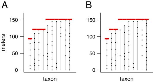
Figure 2 Two possible extinction scenarios with T=10 taxa and p=3 pulses. The scenario in B has range extensions as large or larger than those in A (the range extension for the fourth taxon is larger, and the others are the same), so it is less consistent with the observed fossil record and must therefore have a lower likelihood. Therefore, when finding the most likely scenario, it is not necessary to check the scenario in B, since it cannot possibly be the MLE. Using such shortcuts we avoid computing the likelihood for all possible scenarios, allowing us to find the MLE in a reasonable amount of time.
Our algorithm is as follows:
(i) Find the taxon whose highest fossil occurrence is the highest among all T taxa. Then set the position of the highest pulse equal to the position of that highest fossil occurrence (Fig. 3A).
(ii) From the other T−1 taxa, choose p−1 of them. Then set the positions of the remaining p−1 pulses equal to the positions of the highest fossil occurrence for each of these taxa (Fig. 3B). In the figure, for example, we have T=10 taxa and p=3 pulses, so once we have set the highest pulse to the position of the highest fossil occurrence in the previous step, we then choose two of the nine remaining taxa, and we assign the two remaining pulses to occur at the highest fossil occurrences of these two taxa.
(iii) For each taxon, assign it to the lowest extinction pulse whose position is above (or equal to) that taxon’s highest fossil occurrence (Fig. 3C).
(iv) At this point, we have now uniquely determined a scenario by assigning taxa to pulses. Now calculate its likelihood using equation (2).
(v) Repeat steps (ii)–(iv) until all possible combinations of p−1 taxa have been chosen in step (ii) and their corresponding likelihoods calculated.
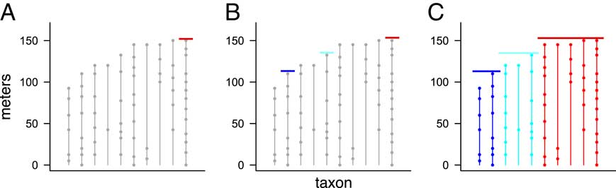
Figure 3 Results of three steps of our efficient algorithm, illustrating how pulses are chosen and taxa assigned to pulses, using a data set with T=10 taxa and p=3 pulses. First, one pulse is set at the position of the highest overall fossil occurrence (A, red line). Next, the positions of the two additional pulses are set by choosing two of the remaining nine taxa, and setting the two pulse positions equal to the position of the highest fossil occurrence in each of these two taxa (B, blue and cyan lines). Finally, each taxon is then assigned to the lowest pulse whose position is above (or equal to) that taxon’s highest fossil occurrence (C, colors indicate taxa assigned to each pulse). See text for details.
This algorithm ensures that for an extinction with T taxa and p pulses, we need only check C(T−1, p−1) possible extinction scenarios. Here C(a, b) denotes the combination function—the number of ways to choose b objects out of a without regard to order—given by C(a, b)=a!/(b! (a−b)!). Because the combination C(T−1, p−1) grows much more slowly as a function of T and p than the Stirling number S(T, p), this algorithm takes substantially less time than checking all possible extinction scenarios. Table 2 (bottom row) gives values of C(T−1, p−1) for T=10 taxa, which are much smaller than the corresponding values of S(T, p) (top row). For T=10, the total number of extinction scenarios checked by this fast algorithm is 1+9+36+…+9+1=512, which is less than 1/200th of the 115,985 total extinction scenarios. For larger numbers of taxa, the time savings is even more dramatic. For example, for T=40 taxa, the number of 5-pulse scenarios to check is given by C(39, 4)=82,251, which is far smaller than the S(40, 5)=7.6×1025 total extinction scenarios.
To explain the algorithm in words: There is a correspondence between an extinction pulse and the taxon whose highest fossil occurrence is the closest to (but below) that pulse position. Therefore, setting the position of p extinction pulses is equivalent to choosing p taxa that correspond to those pulses. We thus conceptualize the algorithm in terms of choosing taxa, rather than setting pulses. The position of the highest pulse is always determined by the taxon whose highest occurrence is the highest among all T taxa, so we need only choose p−1 pulses from the other T−1 taxa. The position of each of these p−1 pulses is set to the position of the highest fossil occurrence for the corresponding taxon. Once these taxa are chosen, it is optimal to assign each remaining taxon to the pulse that is closest to (but above) the taxon’s highest occurrence. In this way, we are able to efficiently calculate MLE p , the most likely extinction scenario having p extinction pulses, for each value of p between 1 and T. In the Appendix, we provide a proof that this efficient algorithm is sufficient compared with searching the entire set of extinction scenarios.
(Note that in the preceding discussion, we have assumed for the sake of expository clarity that there is a single taxon having the highest fossil occurrence in the section. It is possible that more than one taxon may share this distinction. If h taxa are tied for the highest fossil occurrence, the discussion above will still hold if references to T−1 taxa are replaced with T−h. In this case, the computation time of the algorithm will be further reduced.)
Step 2: Comparing the Number of Pulses
At this point, we have determined the most likely scenario for each number of extinction pulses p between 1 and T. We now want to compare these T scenarios in order to find the optimal number of pulses. We cannot simply choose the scenario with the highest likelihood, as the scenario with T pulses will always fit the data best (because it has the most parameters) and thus will have the highest likelihood.
AIC and BIC
Several methods have been developed that attempt to compare likelihoods while taking into account the number of parameters in the model on which the likelihood is based. One such method that has been used in the paleontological literature is AIC (Akaike Reference Akaike1974; Hunt Reference Hunt2006), and a related method is BIC (Schwarz Reference Schwarz1978). We had originally planned to use AIC and BIC directly to compare the likelihoods of the T extinction scenarios. However, tests we ran with simulated data showed that neither AIC nor BIC was effective in predicting the number of extinction pulses with sufficient accuracy. That is, the number of pulses with the best AIC or BIC was often not the actual number of pulses in our simulated data sets.
We decided instead to approach the task of estimating the number of extinction pulses as a classification problem. Classification is a broad field that involves assigning unknown observations to one of a number of discrete categories (e.g., determining whether an e-mail message is legitimate or spam, recognizing the identity of a face in a photograph, reading a handwritten zip code, assigning a new fossil to a particular species). There is a vast literature on classification that spans multiple disciplines (e.g., Hastie et al. Reference Hastie, Tibshirani and Friedman2009), which we do not attempt to review here.
k-Nearest Neighbors
We used the k-nearest neighbor (kNN) algorithm, a well-known classification method (Hastie et al. Reference Hastie, Tibshirani and Friedman2009) (not to be confused with k-means clustering, which is a similarly named but entirely different algorithm). The idea is as follows: first, we create a training set, consisting of a large number of simulated data sets each having a known number of pulses. For each data set in the training set, we use the likelihood equation (2) and our efficient algorithm to calculate the AIC and BIC for each possible number of pulses from 1 to T. This gives us a set of T AIC values and T BIC values for each data set. The T AIC values can be converted into AIC weights that sum to 1 (Anderson et al. Reference Anderson, Burnham and Thompson2000), and the same can be done for the BIC weights; we denote these sets of weights as {AIC1, AIC2, … , AIC T } and {BIC1, BIC2, … , BIC T }. Thus each data set in the training set is associated with a vector of 2T elements, which can be thought of as a set of coordinates in 2T-dimensional space. With a large training set, we will then have a large number of points in 2T-dimensional space, each of which has a known number of pulses. We then take the test set, which in our case is simply the actual data set we wish to analyze. We calculate {AIC1, AIC2, … , AIC T } and {BIC1, BIC2, … , BIC T } for the test set, which determine the coordinates (and thus the location) of the test point in the 2T-dimensional space. If the test point is surrounded in the 2T-dimensional space mostly by training points with a certain number of pulses, then we predict that the test point has that number of pulses as well.
To give an example, we created a training set of 500 simulated data sets having T=10 taxa; these 500 data sets consisted of 100 data sets for each of 1, 2, 3, 4, and 5 pulses. For each simulated data set, we first chose the number of pulses and their positions, simulated the positions of fossil occurrences based on the assumption of uniform preservation and recovery, and then calculated its 20-dimensional vector of AIC and BIC weights based on the fossil occurrences using equation (2). This gave us 500 training points in a 20-dimensional space, each of which has a known number of pulses. Because it is difficult to visualize 20-dimensional space, we show several 2-dimensional snapshots in Figure 4. Of the 500 training data sets, the 100 with 1 pulse are labeled “1” in black, the 100 with 2 pulses are labeled “2” in red, the 100 with 3 pulses are labeled “3” in green, the 100 with 4 pulses are labeled “4” in dark blue, and the 100 with 5 pulses are labeled “5” in orange.
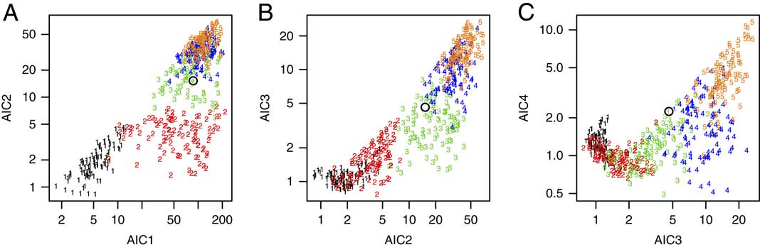
Figure 4 Three views of the 2T-dimensional space used in the kNN algorithm. A, AIC weights for a 2-pulse model (AIC2) plotted against AIC weights for a 1-pulse model (AIC1). B, AIC weights for a 3-pulse model (AIC3) plotted against AIC weights for a 2-pulse model (AIC2). C, AIC weights for a 4-pulse model (AIC4) plotted against AIC weights for a 3-pulse model (AIC3). Each plot has 500 simulated training data sets: 100 each having 1, 2, 3, 4, and 5 pulses. The plotting symbol denotes the number of pulses in each simulated data set (black=1 pulse, red=2 pulses, green=3 pulses, blue=4 pulses, orange=5 pulses). Data sets with the same number of extinction pulses tend to plot in different (although overlapping) regions of the space. The kNN algorithm finds the k points among the training data that are closest to the test data set, calculating the distance in all 2T dimensions (not just in the selected 2-dimensional projections shown here). Axis units are −log(AIC weight).
Figure 4A shows AIC2 plotted against AIC1 (on a logarithmic scale) for the 500 training points; Figure 4B shows AIC3 plotted against AIC2; and Figure 4C shows AIC4 plotted against AIC3. Although there is considerable overlap, it is apparent that extinctions having the same number of pulses tend to cluster in particular regions of the 20-dimensional space.
Having created a training set, we now take the real data set for which we want to estimate the number of extinction pulses, and we calculate its {AIC1, … , AIC10} and {BIC1, … , BIC10} values. Taking these 20 values as coordinates, we plot this point in the 20-dimensional space (Fig. 4, black open circle). Because this point falls in a region populated mostly by training points with three pulses, we therefore conclude that it too most likely had three extinction pulses. In summary, then, kNN works by predicting the class (here, the number of pulses) of a test point as the most common class among its k nearest neighbors among the training points.
We also tried other classification methods such as classification trees (Breiman et al. Reference Breiman, Friedman, Olshen and Stone1984) and a method based on Cobb–Douglas functions from economics (Varian Reference Varian2006). We prefer kNN because it is nonparametric, performed well in our tests, and is fairly fast. Furthermore, it not only predicts the single most likely class, but can also be used to give a distribution of possible answers. For instance, if among the 20 nearest neighbors there are fourteen 3s, five 4s, and a single 1, then we can say that we are 70% confident that the test observation had three pulses, 25% confident that it had 4 pulses, and 5% confident that it had 1 pulse. These proportions may also be interpreted as Bayesian posterior probabilities. Furthermore, we can say that we are 95% confident that there were 3 or 4 pulses, because the individual confidence levels associated with 3 and 4 pulses sum to 95%. Thus kNN has the advantage that it lets us estimate a range of plausible answers rather than simply testing whether a particular prespecified null hypothesis should be rejected or not.
Results from Simulation Studies
To verify that our method works correctly, we ran a series of simulations using randomly generated data sets. All calculations were carried out using the software R (R Core Team 2015).
Simulation Parameters
For each data set, we began by randomly choosing the number of extinction pulses and assigning each taxon to a pulse. We used sample sizes of T=10, 15, 20, 30, 40, and 50 taxa. We then randomly chose the number of fossil occurrences for each taxon from a Poisson distribution with parameter µ (representing the mean number of occurrences per taxon); the value of µ was set to either 7, 10, or 15 for all taxa within a data set. (Note that although µ was constant within a data set, the actual number of occurrences for each taxon was randomly determined based on µ and therefore varied among the taxa.) In addition, the number of occurrences was constrained to fall between 3 and 30 inclusive; randomly chosen values lower or higher than these limits (which were rare) were set to 3 or 30, respectively. The positions of the fossil occurrences for each taxon were then randomly chosen according to a uniform distribution between the base of the stratigraphic section and the position of the assigned extinction pulse, θ i . We then applied our two-step efficient algorithm to each data set thereby generated. For T≤20, we used 1000 random data sets, and for T≥30, we used 500 random data sets, for a total of (3)(3)(1000)+(3)(3)(500)=13,500 simulated data sets.
For these simulations, we limited the maximum number of extinction pulses to four, because usually one would not be interested in distinguishing between large numbers of extinction pulses. For instance, whether a mass extinction had 12 pulses or 13 is not typically of interest; the extinction would be considered gradual either way. The most important distinctions would be for smaller numbers of pulses, such as one versus two, two versus three, and three versus four. In addition, this had the benefit of limiting the running time of the simulations. (In a subsequent section [“Results: Gradual Extinctions”] we will presents results from additional simulations in which the number of extinction pulses is not limited.)
For some extinction scenarios, it may be nearly impossible to discern the number of extinction pulses if the pulses are very close together. For instance, suppose a scenario has four pulses: one at 30 m above the base of the section, another at 60 m, a third at 61 m, and a fourth at 100 m. Unless the number of fossil occurrences is enormous, it will be difficult for any method (or for a human) to distinguish the pulses at 60 and 61 m, and at best the algorithm will find three pulses. (To avoid such situations, in simulations with four or fewer pulses, we constrained the pulses to be separated by at least 20% of the height of the highest possible extinction. For instance, if the extinction pulses were randomly selected to lie between 0 and 100 m above the base of the section, the pulses would have to be separated by at least 20 m. In simulations with five or more pulses, which are described in a subsequent section of the paper [“Results: Gradual Extinctions”], this rule was relaxed so that pulses were allowed to be closer.)
An issue in running the kNN analyses is determining the sample size needed for the training set in step 2 of our algorithm. For kNN what is important is not necessarily to have as large a training set as possible, but rather to make sure that the training set is large enough to “cover” the space with a sufficient density of training points. We ran simulations to determine the necessary size of our training set: we tried values ranging from 100 to 1000 simulated data sets for each possible number of pulses, and decided on 300 simulated data sets per pulse, because we found negligible improvement in using a training set of greater than 300.
Typically in kNN, one uses small values of k (the number of nearest neighbors), such as k=5 or 10, but because our goal is not just to predict the single best class but also to estimate a distribution of possible answers, we used a larger value of k=20 in our simulations. (Using, e.g., k=10 would mean that confidence levels would be rounded to multiples of 10%.) We found in our experiments that the results were not sensitive to the choice of k for k=10, 20, 50, and 100, as long as the number of simulated data sets per pulse (set at 300 in our simulations) was substantially larger than k.
Results: Point Estimates for the Number of Extinction Pulses
Aggregated over all values of T and µ, the method was able to correctly classify the number of extinction pulses with 75% accuracy in the 13,500 simulated data sets. Furthermore, 98.6% of the data sets were predicted within ±1 pulse. However, because our goal is not only to estimate the number of pulses but also our uncertainty in those estimates, what is more important is to assess the confidence levels rather than just the accuracy rate. If the method works correctly, for instance, 65% of all predictions having 65% confidence should be correct, 90% of all predictions having 90% confidence should be correct, and so on. To verify this, we grouped the estimates into bins with confidence levels of 20–29%, 30–39%, … , 90–99%, and 100% (note that with four possible answers, the confidence level cannot be less than 25%). If the method works correctly, then the estimates for data sets falling into these bins should be correct approximately 25%, 35%, … , 95%, and 100% of the time. In fact, the estimates performed as expected (Fig. 5A), showing that our confidence levels are valid. Alternately, in a Bayesian framework, one may think of the confidence levels as posterior probabilities, giving the probability that the number of pulses is estimated correctly.
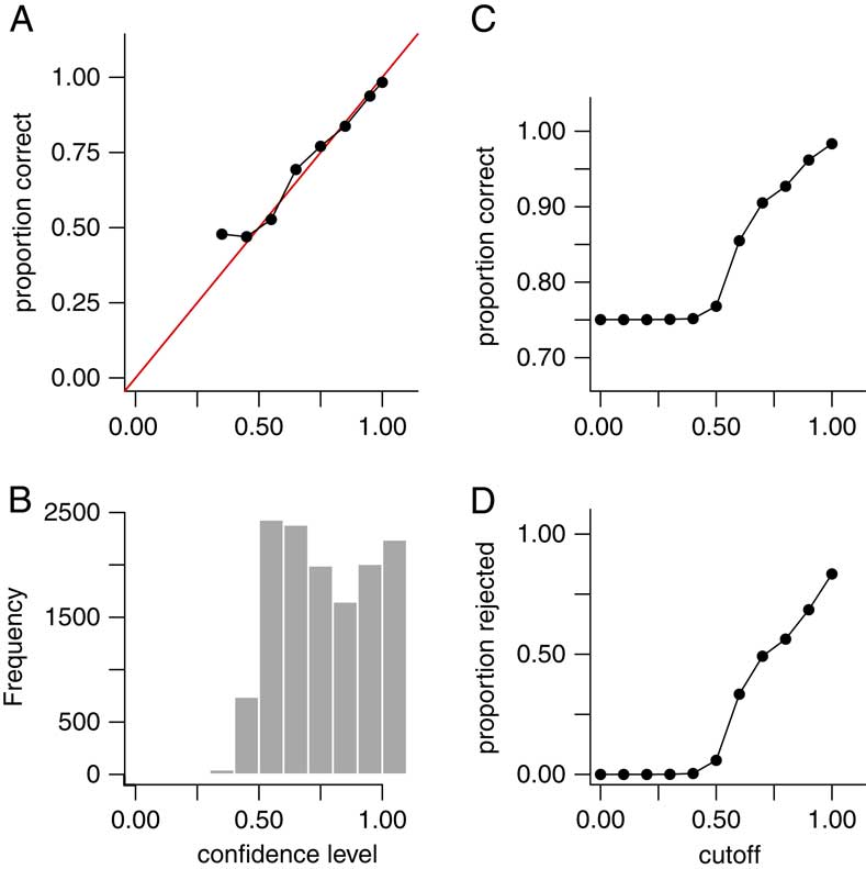
Figure 5 Results for point estimates (predicted number of extinction pulses) in 13,500 simulated data sets aggregated over T=10, 15, 20, 30, 40, and 50 taxa; and µ=7, 10, and 15 mean fossil occurrences per taxon. (Results for individual combinations of parameters (e.g., T=20, µ=7) are similar and are not shown.) The number of extinction pulses was limited to a maximum of four. A, Empirical accuracy rate for point estimates grouped by confidence levels of 20–29%, 30–39%, … , 90–99%, and 100%. Red line is the line y=x. Empirical accuracy for each bin matched the expected value (e.g., data sets with 60–69% confidence had an accuracy rate of close to 65%), except for a minor discrepancy in the 30–39% bin. B, Histogram showing the frequency of each confidence-level grouping. C, Accuracy rate (y-axis) after rejecting data sets with confidence level falling below a given cutoff (x-axis). D, Percent of data sets rejected (y-axis) versus rejection cutoff (x-axis). Accuracy rate increased substantially when ambiguous data sets were excluded. Accuracy rate was 85% for data sets with ≥0.60 confidence, and 93% for data sets with ≥0.80 confidence.
Table 3A shows the results for these 13,500 simulations indexed by T (the number of taxa) and µ (the mean number of fossil occurrences per taxon). The accuracy rate of the method improved slightly as µ increased, although the difference was surprisingly small. The value of T had little effect of on the overall accuracy rate, at least in the range of values that we simulated.
Table 3 Accuracy rates for point estimates as a function of T (number of taxa) and µ (mean number of fossil occurrences per taxon). Accuracy increased slightly for larger values of µ but was fairly similar for all tested values of T. For T≤20 we used 1000 random data sets per simulation, and for T≥30 we used 500 random data sets per simulation, for a total of (3)(3)(1000)+(3)((3)(500)=13,500 simulated data sets. Note that binomial standard error (±1 SE) ranges from approximately 0.006 to 0.014 (depending on the accuracy rate) for a sample size of 1000, and 0.009 to 0.020 for a sample size of 500.
Rejection of Uncertain Data Sets
In many classification situations it is common to attempt to classify only those data sets in which we are confident of a correct answer, and decline or reject the remaining data sets. In our context, this corresponds to attempting to estimate the number of pulses only for data sets for which the confidence level is above some threshold or cutoff. For example, if our method gives a low confidence level for a data set, it may be the case that the data set is inherently difficult to classify because the true extinction pulses are close together, or because some taxa have too few fossil occurrences. We can then reject such data sets and decline to estimate their number of pulses. Figure 5B gives a histogram of estimated confidence levels for the simulated data sets, showing how often various confidence levels were achieved; Fig. 5C shows the accuracy rate in our 13,500 simulated data sets as a function of the rejection cutoff value; and Fig. 5D shows the percent of the simulated data sets that are rejected using a given cutoff. Overall, if we reject the 35% of data sets for which the confidence level is below 0.60, the accuracy rate of the remaining data sets rises to 85%. If we reject the 58% of data sets for which the confidence level is below 0.80, the accuracy rate of the remaining data sets further rises to 93%. Thus, rejection of ambiguous data sets does increase accuracy rates, but with the trade-off that a lower percentage of data sets is classified. Table 3B,C gives accuracy rates for rejection using cutoffs of 0.60 and 0.80 as a function of T and µ. As seen previously with the complete data set, accuracy rates improve slightly as µ increases but do not seem to be sensitive to the value of T.
Results: Confidence Intervals
We also tested whether the empirical coverage probabilities of our confidence intervals matched their nominal confidence levels—for example, whether our 90% confidence intervals actually contained the correct answer in at least 90% of data sets. Note that because our confidence intervals are discrete sets rather than continuous intervals, it is not always possible to obtain an interval with an exact prespecified confidence level. For instance, if the kNN classifier returns 0.85 confidence for a single pulse and 0.15 for two pulses, then we can obtain only 100%, 85%, and 15% confidence intervals. Furthermore, because we used k=20 in the kNN classifier, in our simulations we can obtain only confidence levels that are multiples of 5% (i.e., 1/20). Thus, our intended 90% confidence intervals may turn out to have 90%, 95%, or 100% confidence. However, in such cases, we always consider the resulting interval to be a 90% confidence interval, because 90% was the level of confidence specified at the outset of the analysis.
In our 13,500 simulated data sets with 1–4 pulses, our 90% confidence interval contained the true number of pulses 97.6% of the time. Moreover, the empirical coverage probability was at least 90% for each number of pulses tested (Fig. 6). Thus, confidence intervals produced by our method did indeed attain their nominal confidence levels; in fact, they were somewhat over-conservative.
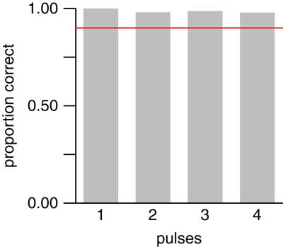
Figure 6 Empirical coverage probabilities for 90% confidence intervals applied to the same 13,500 simulated data sets as in Fig. 5. Red line denotes 90% coverage probability. For each number of pulses, confidence intervals contained the true value in at least 90% of data sets.
Results: Gradual Extinctions
In the simulations reported above, we tested scenarios having only 1 to 4 extinction pulses—that is, scenarios that were simultaneous or having only a small number of pulses. We also conducted simulations that allowed more gradual scenarios, with all possible numbers of pulses from 1 to T for T taxa. (Here we use “gradual” in an informal sense to refer to any scenario with a large number of pulses relative to the number of taxa.) We simulated data sets with T=10 taxa, and a mean number of occurrences per taxon of either µ=10 or 20. (As before, the actual number of occurrences for each taxon was randomly chosen according to a Poisson distribution with the given mean µ.) For each possible number of pulses and each value of µ, we simulated 500 data sets, for a total of (10)(2)(500)=10,000 simulated data sets. This is a more restricted set of parameter values than was used in the previously described simulations, as testing larger numbers of pulses is computationally intensive. We also used only larger average sample sizes (i.e., larger values of µ), because it is not feasible to distinguish large numbers of pulses when each taxon has few occurrences. When µ=20, the method performed as expected for all possible numbers of pulses, with the empirical coverage probability always exceeding the nominal level of 90% (Fig. 7B). For µ=10, the method performed as expected for 1–4 pulses, which confirms the results described above (Fig. 6), and also performed well for 9–10 pulses, but was slightly below its nominal confidence level for 5–8 pulses (Fig. 7A). In summary, for smaller numbers of pulses, the method worked well and was especially accurate at identifying simultaneous, 2-pulse, or 3-pulse scenarios. For larger numbers of pulses, the method worked well with large sample sizes (larger numbers of occurrences per taxon), but less so with smaller sample sizes. Finally, the method worked well for scenarios that were completely gradual or nearly so.
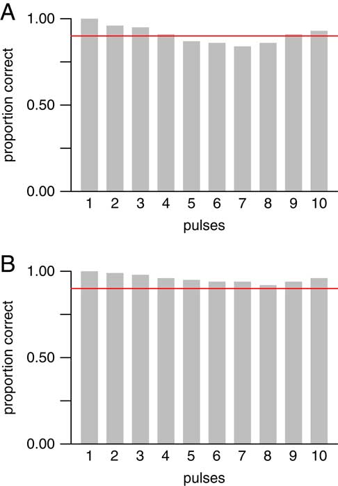
Figure 7 Empirical coverage probabilities for 90% confidence intervals in 10,000 simulated data sets with T=10 taxa, and µ=10 (A) or 20 (B) mean number of occurrences per taxon. All possible numbers of pulses from T=1 to 10 were allowed. Red line denotes 90% coverage probability. For µ=10 (A), confidence intervals contained the true value in at least 90% of data sets for 1–4 and 9–10 pulses, but performed slightly worse than expected for 5–8 pulses. For µ=20 (B), confidence intervals contained the true value in at least 90% of data sets for all numbers of pulses. Thus, the method worked well for smaller numbers (1–4) of pulses and very gradual extinctions (9–10 pulses), but required larger sample sizes to work well for 5–8 pulses.
An Illustrative Example: Late Cretaceous Ammonites
We illustrate the algorithm using data on 10 ammonite species from the latest Cretaceous of Seymour Island, Antarctica (Macellari Reference Macellari1986). Because several species do not appear to be present lower in the section, we limit our attention to fossils occurring higher than 1000 m above the base of the section. This data set has been widely used as an illustrative example in the literature, because it is one of the few for which the assumption of uniform preservation and recovery may be plausible. Strauss and Sadler (Reference Strauss and Sadler1989) argued that uniformity is reasonable based on lithology, collection strategy, and statistical tests of gap lengths. Marshall (Reference Marshall1995a) argued similarly and showed that the distribution of fossil occurrences is consistent with uniformity based on a Kolmogorov–Smirnov test (it is worth noting, however, that this test can have low power at the small sample sizes used here). Wang et al. (Reference Wang, Chudzicki and Everson2009: Fig. 2D) used a more powerful graphical method, the uniform probability plot, to show that the distribution of fossil occurrences closely matched what would be expected from a uniform distribution.
Several authors (Strauss and Sadler Reference Strauss and Sadler1989; Springer Reference Springer1990; Solow Reference Solow1996; Solow and Smith Reference Solow and Smith2000) have concluded that the pattern of occurrences is consistent with a simultaneous extinction. Marshall (Reference Marshall1995a) concluded that the pattern of fossil occurrences is consistent with both a simultaneous extinction and a range of gradual extinctions occurring over up to 20 m of stratigraphic thickness. In our companion paper (Wang et al. Reference Wang, Chudzicki and Everson2012), we found that the 90% confidence interval for the duration of this extinction is from 0 to 62 m. In other words, both a sudden extinction (corresponding to a duration of 0 m) and a gradual extinction (occurring over as much as 62 m) are plausible.
Results from our new method are consistent with these previous results. Here we find that the pattern of occurrences is best supported by a simultaneous extinction, but a two-pulse scenario receives some support as well, whereas scenarios having three or more pulses have little to no support (Fig. 8). The top row of Figure 8 shows the most likely positions of extinction pulses for scenarios having one through six extinction pulses (i.e., MLE1 through MLE6 of step 1). The bottom row shows the confidence level for each of these numbers of pulses as determined by the kNN algorithm (step 2). (Results for 7 through 10 pulses were calculated but are not shown because they had a confidence level of zero.) We can thus say with 90% confidence that the extinction occurred in a single pulse.
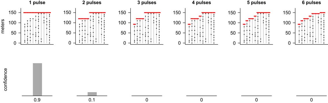
Figure 8 MLEs for 1–6 pulse extinction scenarios (top row) for ammonite species (T=10 species) from the latest Cretaceous of Seymour Island, Antarctica (Macellari Reference Macellari1986; Marshall Reference Marshall1995a) and corresponding confidence levels (bottom row). Results for scenarios with more than six pulses were computed but had zero confidence and are not shown. A single-pulse extinction event was strongly favored, although there was weak support for a two-pulse extinction. We can state with 90% confidence that the extinction occurred in a single pulse.
This example took about 13 seconds to run on an Apple MacBook Pro (2013 Core i7 model). Calculations were carried out using the software R; computer code is available in the online Supplementary Material.
Sensitivity to Model Assumptions
Sensitivity to the Assumption of Uniform Preservation and Recovery
We have assumed uniform preservation and recovery of fossils throughout their true stratigraphic ranges, an assumption commonly made in the literature (Strauss and Sadler Reference Strauss and Sadler1989; Springer Reference Springer1990; Marshall Reference Marshall1990, Reference Marshall1995a; Marshall and Ward Reference Marshall and Ward1996; Solow Reference Solow1996; Weiss and Marshall Reference Ward, Botha, Buick, de Kock, Erwin, Garrison, Kirschvink and Smith1999; Solow and Smith Reference Solow and Smith2000; Jin et al. Reference Jin, Wang, Wang, Shang, Cao and Erwin2000; Ward et al. Reference Wang, Everson, Zhou, Park and Chudzicki2005; Solow et al. Reference Solow, Roberts and Robbirt2006; Groves et al. Reference Groves, Rettori, Payne, Boyce and Altiner2007; Wang and Everson Reference Wang and Everson2007; Lindström and McLoughlin Reference Lindström and McLoughlin2007; Wang et al. Reference Wang, Chudzicki and Everson2009, Reference Wang, Chudzicki and Everson2012; Angiolini et al. Reference Angiolini, Checconi, Gaetani and Rettori2010; Tobin et al. Reference Tobin, Ward, Steig, Olivero, Hilburn, Mitchell, Diamond, Raub and Kirschvink2012; Song et al. Reference Song, Wignall, Tong and Yin2013; He et al. Reference He, Shi, Twitchett, Zhang, Zhang, Song, Yue, Wu, Wu, Yang and Xiao2015; Garbelli et al. Reference Garbelli, Angiolini, Brand, Shen, Jadoul, Posenato, Azmy and Cao2015). This assumption is akin to that of an ideal gas in chemistry, a perfect market in economics, or a point mass in physics—perhaps a useful idealization, but one that is never true in real life.
Research over the past several decades has made substantial advances in understanding the effect of environmental factors and stratigraphic architecture on the spatial and temporal distribution of taxa, and thus the probability of preservation and recovery of fossils (Patzkowsky and Holland Reference Patzkowsky and Holland2012). Gradients in environmental factors such as water depth (Holland and Patzkowsky Reference Holland and Patzkowsky2004; Scarponi and Kowalewski Reference Scarponi and Kowalewski2004; Amati and Westrop Reference Amati and Westrop2006; Olabarria Reference Olabarria2006; Konar et al. Reference Konar, Iken and Edwards2008; Smale Reference Smale2008), substrate consistency (Scarponi and Kowalewski Reference Scarponi and Kowalewski2004; Holland and Patzkowsky Reference Holland and Patzkowsky2007), and salinity (Horton et al. Reference Horton, Edwards and Lloyd1999) are known to correlate with the distribution of marine taxa, thereby influencing recovery potential. Sequence stratigraphic principles have also informed our understanding of the distribution of fossils, such as the size of range offsets (Holland and Patzkowsky Reference Holland and Patzkowsky2002) and the clustering of first and last occurrences around sequence boundaries (Holland Reference Holland1995, Reference Holland2000; Holland and Patzkowsky Reference Holland and Patzkowsky2009, Reference Holland and Patzkowsky2015). Given these and other factors influencing recovery potential, it is unrealistic to suppose that they would all cancel out to result in a data set with truly uniform recovery potential.
Results based on the assumption of uniformity are likely to be incorrect when the true recovery potential is not close to uniform (Holland Reference Holland2003; Solow Reference Solow2003; Rivadeneira et al. Reference Rivadeneira, Hunt and Roy2009; Wang et al. Reference Wang, Chudzicki and Everson2009). To examine how well our method works under such circumstances, we conducted a sensitivity analysis. We simulated data sets based on the reflected beta distribution, which was introduced by Wang et al. (Reference Wang, Wang, Gai, Moore, Porter and Maloof2016) to model nonuniform recovery potential. This distribution can take on a variety of monotonically increasing or decreasing shapes, governed by the parameter λ. A value of λ=0 corresponds to uniform recovery potential. A value of λ>0 corresponds to increasing recovery potential (i.e., the probability of recovering fossils increases toward the time of extinction, as might be expected of a taxon that is diversifying until it is extirpated in a sudden extinction event). A value of λ<0 corresponds to decreasing recovery potential (i.e., the probability of recovering fossils decreases toward the time of extinction, as might be expected of a taxon gradually declining in abundance until it goes extinct). We simulated data sets based on the values λ=0, ±0.5, and ±1. For each of these five values of λ, we simulated 3600 data sets, comprising 100 data sets for each of µ=7, 10, and 15 mean occurrences per taxon; T=10, 20, and 30 taxa; and p=1, 2, 3, or 4 pulses; for a total of (5)(3)(3)(4)(100)=18,000 simulated data sets. We then examined the accuracy of our point estimates and confidence intervals for each value of λ, aggregated over the other parameters (Fig. 9).
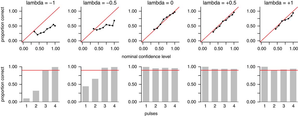
Figure 9 Sensitivity analysis showing accuracy of point estimates and confidence intervals under nonuniform recovery potential. Top row shows accuracy rates for point estimates (predicted number of pulses); plot format is the same as Fig. 5A. Bottom row shows empirical coverage probabilities for confidence intervals; plot format is the same as Fig. 6. Columns represent values of λ, a parameter governing the shape of the recovery function in the reflected beta distribution (Wang et al. Reference Wang, Wang, Gai, Moore, Porter and Maloof2016). Values of λ<0 correspond to decreasing recovery potential toward the time of extinction (left two columns); λ=0 corresponds to uniform recovery potential (middle column); and λ>0 corresponds to increasing recovery potential toward the time of extinction (right two columns). The method performed well under uniform recovery potential and increasing recovery potential, but poorly when recovery potential is decreasing.
As shown above, the method performs well when λ=0, corresponding to uniform recovery potential (Fig. 9, center column). Point estimates achieve their nominal confidence levels within sampling error (top row), as do confidence intervals for each number of pulses (bottom row). The method also works well when recovery potential is increasing (rightmost two columns). However, when recovery potential is decreasing (leftmost two columns), the method works poorly. Point estimates do not achieve their nominal confidence levels, and confidence intervals fall short of their nominal confidence levels for one- and two-pulse scenarios, although they do work for three- and four-pulse scenarios. In other words, when recovery potential is decreasing, the method overestimates the correct number of pulses. Thus, our method should be used only in cases in which recovery potential is known or estimated to be uniform or increasing. This clearly limits the method’s utility, as it is likely that decreasing recovery potential is more common in the fossil record than increasing or uniform recovery (although in the specific context that our method is designed to address—a mass extinction that is suspected of occurring in a small number of sudden pulses—one might argue that increasing or uniform recovery might be more common than it is in the fossil record in general). Regardless, it is clear that the method does not perform reliably when recovery potential is decreasing.
Sensitivity to the Assumption of Continuous Sampling
We have also assumed that fossils are sampled continuously within the taxon’s true stratigraphic range. This assumption is commonly made in the literature, either explicitly or implicitly (Strauss and Sadler Reference Strauss and Sadler1989; Marshall Reference Marshall1990, Reference Marshall1995a; Springer Reference Springer1990; Marshall and Ward Reference Marshall and Ward1996; Solow Reference Solow1996; Jin et al. Reference Jin, Wang, Wang, Shang, Cao and Erwin2000; Solow and Smith Reference Solow and Smith2000; Ward et al. Reference Wang, Everson, Zhou, Park and Chudzicki2005; Solow et al. Reference Solow, Roberts and Robbirt2006; Groves et al. Reference Groves, Rettori, Payne, Boyce and Altiner2007; Lindström and McLoughlin Reference Lindström and McLoughlin2007; Wang and Everson Reference Wang and Everson2007; Wang et al. Reference Wang, Chudzicki and Everson2009, Reference Wang, Chudzicki and Everson2012; Angiolini et al. Reference Angiolini, Checconi, Gaetani and Rettori2010; Tobin et al. Reference Tobin, Ward, Steig, Olivero, Hilburn, Mitchell, Diamond, Raub and Kirschvink2012; Song et al. Reference Song, Wignall, Tong and Yin2013; Garbelli et al. Reference Garbelli, Angiolini, Brand, Shen, Jadoul, Posenato, Azmy and Cao2015; He et al. Reference He, Shi, Twitchett, Zhang, Zhang, Song, Yue, Wu, Wu, Yang and Xiao2015). In reality, however, virtually all sampling is discrete, either because fossil occurrences are confined to individual beds or bedding planes or simply because data cannot be measured with infinite precision and can therefore take on only a limited number of values. Such discretization causes dependence among the positions of fossil occurrences of different taxa, which are assumed to be independent. Wang et al. (Reference Wang, Chudzicki and Everson2009) investigated the effect of such violations of independence, finding that it is relatively smallest when recovery potential is uniform and potentially more severe otherwise. In practice, if the number of possible discrete values is relatively large, the effect of such discretization will be minimized, and the assumption of continuous sampling will be more reasonable (Payne Reference Payne2003).
To examine how well our method works under discrete sampling, we applied the method to data sets simulated with fossil occurrences falling between 0 and θ=100 as described above, but with the positions of all fossil occurrences rounded to the nearest 5 units to mimic the effect of discrete sampling. We simulated 100 data sets for each of µ=7, 10, and 15 mean occurrences per taxon; T=10, 20, and 30 taxa; and p=1, 2, 3, or 4 pulses; for a total of (3)(3)(4)(100)=3600 simulated data sets. Recovery potential was assumed to be uniform. We then examined the accuracy of our point estimates and confidence intervals aggregated over all parameter values (Fig. 10). Our point estimates achieve the confidence levels returned by the kNN classifier (Fig. 10A), and our confidence intervals achieve their nominal confidence levels (Fig. 10B).
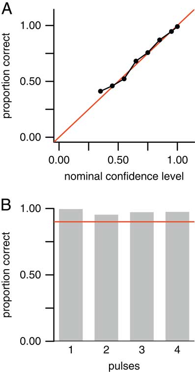
Figure 10 Sensitivity analysis showing accuracy of point estimates and confidence intervals under discrete sampling. Positions of fossil occurrences were randomly generated between 0 and 100 units, then rounded to the nearest 5 units to simulate discrete rather than continuous sampling. A, Accuracy rates for point estimates (predicted number of pulses); plot format is the same as Fig. 5A and top row of Fig. 9. B, Empirical coverage probabilities for confidence intervals; plot format is the same as Fig. 6 and bottom row of Fig. 9. The method performed well under this level of discretization.
Sensitivity to Other Assumptions
We performed a number of additional simulations intended to assess the robustness of our method:
1. We simulated data sets where each taxon’s sample size was randomly chosen from a Poisson distribution with mean µ=5, to assess performance when the number of fossil occurrences is small.
2. We simulated data sets where each taxon’s sample size was randomly chosen from a Poisson distribution with mean µ in which the values of µ were themselves randomly chosen (as opposed to the simulations described earlier in which µ was set to the same value for all taxa).
3. We simulated data sets in which each taxon’s sample size was randomly chosen directly between a specified lower and upper limit (here set to 3 and 30 taxa, respectively), without using a Poisson distribution.
4. We simulated data sets where the number of taxa was limited to 8, to assess performance when the number of taxa per extinction pulse is small.
The method worked as intended under these situations; the results were similar to those in Figure 10 and are not shown here.
Discussion
Most previous work on the Signor–Lipps effect has focused on testing whether an extinction event was sudden or gradual. In a companion paper (Wang et al. Reference Wang, Chudzicki and Everson2012) and in the present paper, we have attempted to broaden the question by asking how gradual the extinction could have been, and how many pulses it could have encompassed. In both cases, the goal is to shift the focus from testing whether the fossil record is or is not consistent with a particular scenario, to identifying the range of scenarios with which the fossil record is consistent.
We have defined a pulse as a unique time or stratigraphic position of an extinction shared by one or more taxa. This definition may or may not always match a researcher’s intuitive definition of a pulse. For example, we are estimating the number of pulses without regard for the size of each pulse. It is possible for a single taxon to constitute a pulse by itself (Fig. 2A), although some researchers might not consider the extinction of a single taxon as being a “pulse.” Moreover, it is possible for the method to identify pulses that are so close together that most researchers would consider them a single pulse (Fig. 11). It is thus important to examine the sizes and positions of the estimated pulses before coming to any conclusions.
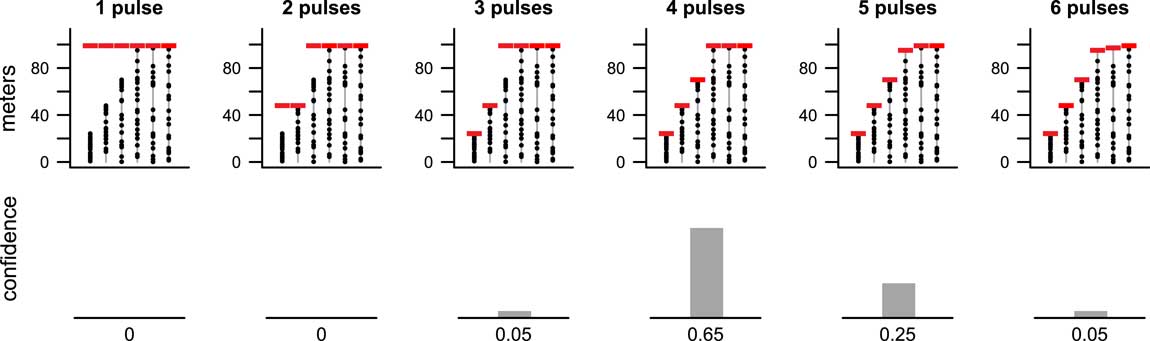
Figure 11 Results from a simulated data set with three taxa going extinct due to background extinctions, followed by an extinction pulse killing the three remaining taxa. The true extinction levels were θ1=25 m, θ2=50 m, θ3=75 m, and θ4=θ5=θ6=100 m above the base of the section, so there is a total of four pulses. We then simulated positions of fossil occurrences from this scenario, assuming 20 occurrences for each taxon. The method correctly estimated that there were four pulses, but some weight was given to a five-pulse scenario as well. However, in the five-pulse scenario, the position of the fifth pulse was so close to that of the fourth pulse that most researchers would likely consider this a four-pulse extinction.
We have focused on estimating the number of extinction pulses rather than their positions. However, if the positions are of interest as well, our method also yields estimates of the positions for each number of pulses (Fig. 8). These positions are the MLEs, which are biased downward in this situation (Strauss and Sadler Reference Strauss and Sadler1989). Assuming uniform recovery, better estimates of the pulse positions can be found using the methodology of Wang et al. (Reference Wang, Chudzicki and Everson2009), which estimates the true time of extinction of a collection of taxa by pooling them into one combined “supersample.” If the taxa estimated to have gone extinct in pulse p have a total of n (p) occurrences among them, then the best unbiased estimate of their common extinction time is the position of the highest fossil occurrence among the taxa multiplied by (n (p)+1)/n (p) (Wang et al. Reference Wang, Chudzicki and Everson2009). If uniform recovery is not assumed, then methods such as that of Wang et al. (Reference Wang, Wang, Gai, Moore, Porter and Maloof2016) may be used to estimate the positions of the pulses.
Our method can in principle also be applied to origination events, which are mathematically equivalent to extinction events but in the opposite direction. With appropriate data sets, it may be possible to estimate the number of origination pulses in events such as the Cambrian explosion (Wang et al. Reference Wang, Zimmerman, McVeigh, Everson and Wong2014) or the Ordovician radiation. However, for origination, the assumption of uniform recovery is less likely to hold than it is for extinction. In the latter case, one might conceivably be able to argue that recovery potential could be uniform for taxa having steady abundance in a constant environment, until being wiped out in a sudden extinction. But in the case of origination, taxa are necessarily increasing in abundance and geographic range from their time of origination. As a result, recovery potential should be decreasing toward the time of origination, in which case the method will be unreliable.
The fact that our method does not work well when recovery potential is decreasing is an important limitation. One might therefore argue that the novelty of our method is at this point more conceptual than practical. Extending our method to accommodate nonuniform recovery potential is not straightforward and presents substantial algorithmic and computational challenges. Overcoming these obstacles is a current goal of work in our research group.
In conclusion, previous methods have focused on testing whether an extinction event occurred in one pulse or many. Here our goal is to ask instead, how many? It is possible for both “one” and “many” to be plausible answers to this question, a situation that is not adequately captured in a hypothesis testing framework. With the caveat that the model assumptions must be satisfied, our methodology is therefore better able to capture the range of scenarios that is consistent with the observed fossil record.
Acknowledgments
We thank S. Chang, P. Everson, I. Fellows, G. Hunt, J. Lin, E. Magenheim, C. Pattanayak, A. Ruether, P. Wagner, D. Wang, L. Yang, and H. Zhou for their assistance. We also thank S. Porter for suggesting the idea for this paper and for reading a draft of the manuscript, and L. Chen, C. Grood, T. Hunter, S. Maurer, and W. Stromquist for help with Stirling numbers. Additionally, we thank Steven Holland, Shanan Peters, and two anonymous referees for thoughtful and constructive reviews that substantially improved the paper, and B. MacFadden for his guidance during the submission process. Funding to principal investigator S.C.W. from National Science Foundation award EAR-0922201 and the Swarthmore College Research Fund and James Michener Faculty Fellowship is gratefully acknowledged. We are also grateful for additional funding provided by the Lotte Lazarsfeld Bailyn ’51 Research Endowment from Swarthmore College, the Howard Hughes Medical Institute, Sigma Xi, and the Swarthmore College Department of Mathematics and Statistics.
Supplementary Material
Data available from the Dryad Digital Repository: http://dx.doi.org/10.5061/dryad.cj38k
Appendix: Proof of Sufficiency of the Algorithm
Here we show that our efficient algorithm is sufficient to find the maximum likelihood extinction scenario. Suppose we are given any possible extinction scenario with some given T and p such that the number of distinct values in {y 1, y 2, … , y T } is at least p. We should be able to say it is either in L T,p , the set of all scenarios we check for that specific T and p, or else say its likelihood is no larger than a particular scenario in L T,p .
Suppose we are given an extinction scenario Ω u with T taxa and p pulses, which is characterized by extinction positions {θ u,1, θ u,2, … , θ u,T }. Then it has a corresponding vector of pulse positions {φ u,1, φ u,2, … , φ u,p }. To be a possible scenario, Ω u must satisfy max{φ u,1, φ u,2, … , φ u,p }= max{y 1, y 2, … , y T }. To be a scenario with p pulses, it must be true that φ u,i ≠ φ u,j for all i ≠ j. Given these statements, we make two claims here:
Claim 1: Suppose there exists a pulse position φ u,a >y j , such that φ u,a ≠ θ u,i for i=1, 2, … , T. Let A be the set of all j such that θ u,j =φ u,a . There exists Ω v , another scenario in which θ v,i =θ u,i , except that θ v,j = max j ∈ A {y j }. We claim Ω v has a higher likelihood than Ω u .
Proof: by equation (2) (copied below) we can write down the log-likelihood of scenarios u and v, and the only difference in log-likelihoods is θ v,j of all j in A.
 $$\eqalignno{&{\rm log}\;L({\rm \theta }_{1} \,\ldots\,{\rm \theta }_{T} ){\equals} \cr \mathop{\sum}\limits_{i{\equals}1}^T {{\rm log}(n_{i} (y_{i} \,/\,{\rm \theta }_{i} )^{{n_{i} {\minus}1}} )}$$
y i ≤θ i for all i.
We take the difference between these two log-likelihoods and compare it with 0:
 $$\eqalign{& \log \;L({\rm \theta }_{{_{v} ,1}} ,\!\!\;\ldots\;\!\!,{\rm \theta }_{{v,T}} ) \cr {\minus}\log \;L({\rm \theta }_{{u,1}} ,\;\,\!\!\!\ldots\!\!\!\,\;,{\rm \theta }_{{u,T}} ) {\equals} \cr \mathop{\sum}\limits_{j\inA}^{} {\{ \log [n_{j} \cdot (y_{j} \,/\,{\rm \theta }_{{v,j}} )^{{nj{\minus}1}} ] }\cr {{\minus}\log [n_{j} \cdot (y_{j} \,/\,{\rm \theta }_{{u,j}} )^{{n_{j} {\minus}1}} ]\} } \cr {\equals}{\rm log}[({\rm \theta }_{{u,j}} \,/\,{\rm \theta }_{{v,j}} )^{{n_{j} {\minus}1}} ] $$
Because of the way we constructed Ω v we know that θ u,j >θ v,j for all j in A, and thus log[(θ u,j /θ v,j ) nj −1]>0 for all j in A. Therefore the difference is positive, which means the log-likelihood of Ω v is greater than the log-likelihood of Ω u .
Claim 2: Suppose there exists a taxon a such that there exists φ u,h , such that y u,a ≤φ u,h <θ u,a . Then we claim Ω v , a scenario in which θ v,i =θ u,i except that θ v,a =φ u,h has a higher likelihood.
Proof: If we consider the difference in log-likelihood of scenarios u and v again, we have the following:
 $$\eqalignno{&{\rm log}\;L({\rm \theta }_{{v,1}} ,\!\!\;\ldots\;\!\!\!\!\;,\!{\rm \theta }_{{v,T}} ){\minus}{\rm log}\;L({\rm \theta }_{{u,1}} ,\!\!\;\ldots\;\!\!,{\rm \theta }_{{u,T}} ){\equals} \cr {\rm log[}({\rm \theta }_{{u,a}} \,/\,{\rm \theta }_{{v,a}} )^{{n_{a} {\minus}1}} ]$$
Because of the way we constructed Ω v we know that θ u,a >θ v,a , and thus the difference is positive, which means the log-likelihood of Ω v is greater than the log-likelihood of Ω u .
If any of the above applies to Ω u , then replace Ω u by Ω v constructed in the corresponding claim, then check if any of the above applies to Ω v . We loop over these claims and continue improving the scenario, until none of the above applies. We claim, and show below, that the final scenario we obtain from the loop is in L T,p .
If none of the above applies to Ω u , then Ω u must be in L T,p , because we can obtain it by the efficient algorithm as follows:
1. Let φ u,p =max{y 1, y 2, … , y T }.
2. There must exist a subset of {y 1, y 2, … , y T } that consists of p−1 distinct elements with every element strictly smaller than φ u,p . If we call this subset {y a1, y a2, … , y a(p–1)}, then we can let φ u,1 =y a1, φ u,2 =y a2, and so on.
3. For i=1, 2, … , T, let θ u,i =min c {φ u,c | φ u,c ≥y i }.
4. Ω u is characterized by {θ u,1 , θ u,2 , … , θ u,T }.
Thus this algorithm is sufficient to find the maximum likelihood scenario for given T and p.


