


Introduction
Patterns of stability and change in community structure through time, and the processes that drive such patterns, represent an area of significant interest in the fields of ecology and macroevolution (e.g., Paine Reference Paine1969; Connell and Slatyer Reference Connell and Slatyer1977; Vrba Reference Vrba1985, Reference Vrba1992, Reference Vrba1993; Eldredge Reference Eldredge, Adrain, Edgecombe and Lieberman2001; Mougi and Kondoh Reference Mougi and Kondoh2012). It is generally presumed that abrupt and significant ecological change ultimately leads to cascading extinction with subsequent community collapse. Yet the fossil record has repeatedly demonstrated that, despite changes in the environment, the composition of paleocommunities (sensu Bennington and Bambach Reference Bennington and Bambach1996) can remain remarkably stable over periods that stretch from thousands to millions of years (Grabau Reference Grabau1898; Cleland Reference Cleland1903; Vrba Reference Vrba1992; Brett and Baird Reference Brett, Baird, Erwin and Anstey1995; Morris et al. Reference Morris, Ivany, Schopf and Brett1995). The key question is: to what degree are these paleocommunities truly stable, as opposed to just generally similar? (Bennington and Bambach Reference Bennington and Bambach1996; Brett et al. Reference Brett, Ivany and Schopf1996; Holterhoff Reference Holterhoff1996; Ivany Reference Ivany1996; Jablonski and Sepkoski Reference Jablonski and Sepkoski1996; Lieberman and Kloc Reference Lieberman and Kloc1997; Miller Reference Miller1997; Patzkowsky and Holland Reference Patzkowsky and Holland1997; Olszewski and Patzkowsky Reference Olszewski and Patzkowsky2001a,Reference Olszewski and Patzkowskyb; Bonuso et al. Reference Bonuso, Newton, Brower and Ivany2002a,b; Pandolfi Reference Pandolfi2002; Bonelli et al. Reference Bonelli, Brett, Miller and Bennington2006; Ivany et al. Reference Ivany, Brett, Wall, Wall and Handley2009; Balseiro Reference Balseiro2016; Antell et al. Reference Antell, Kiessling, Aberhan and Saupe2020). An obvious follow-up question also presents itself: if communities are stable, what factors allow them to remain so despite changes in environmental conditions?
The considerable attention paid to the question of community stability and its possible drivers may be due to the broader implications of the results. For example, whether changes in the structure of communities do or do not track shifts in the environment directly bears on understanding the role incumbency plays in mediating community structure (Reymond et al. Reference Reymond, Bode, Renema and Pandolfi2011; Roopnarine et al. Reference Roopnarine, Angielczyk, Weik and Dineen2019), how competition and biotic interactions may influence community composition (Hairston et al. Reference Hairston, Smith and Slobodkin1960; Tilman Reference Tilman1982; Gallien Reference Gallien2017), and whether the origination and extinction of species is largely driven by ecosystem change (Rundell and Price Reference Rundell and Price2009; Condamine et al. Reference Condamine, Rolland and Morlon2013). The last possibility has led to the development of concepts such as “turnover pulse” (Vrba Reference Vrba1985, Reference Vrba1992, Reference Vrba1993) and the “sloshing bucket” (Eldredge Reference Eldredge, Adrain, Edgecombe and Lieberman2001) in an attempt to characterize and explain the evolutionary implications of long-term community stability.
The potential archetype of stable paleocommunities is the marine invertebrate fauna from the Middle Devonian Hamilton group of New York State (Brett and Baird Reference Brett, Baird, Erwin and Anstey1995). This fauna serves as the type example of the phenomenon known as “coordinated stasis” (Brett and Baird Reference Brett, Baird, Erwin and Anstey1995; Morris et al. Reference Morris, Ivany, Schopf and Brett1995). Coordinated stasis posits that, at the scale of regional biotas, persistent paleocommunity composition is the default, until it is ultimately interrupted by an associated rapid turnover event involving extinction of preexisting species, the migration or evolution of new species, and the reconstitution of a new functionally and taxonomically distinct paleocommunity. However, whether coordinated stasis holds for the Middle Devonian of New York State, or in other regions and time periods, has been much debated (Brett and Baird Reference Brett, Baird, Erwin and Anstey1995; Morris et al. Reference Morris, Ivany, Schopf and Brett1995; Bennington and Bambach Reference Bennington and Bambach1996; Brett et al. Reference Brett, Ivany and Schopf1996; Holterhoff Reference Holterhoff1996; Ivany Reference Ivany1996; Jablonski and Sepkoski Reference Jablonski and Sepkoski1996; Lieberman and Kloc Reference Lieberman and Kloc1997; Miller Reference Miller1997; Patzkowsky and Holland Reference Patzkowsky and Holland1997; Olszewski and Patzkowsky Reference Olszewski and Patzkowsky2001a,Reference Olszewski and Patzkowskyb; Bonuso et al. Reference Bonuso, Newton, Brower and Ivany2002a,Reference Bonuso, Newton, Brower and Ivanyb; Pandolfi Reference Pandolfi2002; Bonelli et al. Reference Bonelli, Brett, Miller and Bennington2006; Ivany et al. Reference Ivany, Brett, Wall, Wall and Handley2009; Balseiro Reference Balseiro2016; Antell et al. Reference Antell, Kiessling, Aberhan and Saupe2020).
To consider these topics further, we use as our touchstone the detailed fossil record of Carboniferous (Pennsylvanian) brachiopod assemblages from the Midcontinent of North America. These were highly diverse assemblages that persisted in an exceptionally dynamic environmental setting. In particular, these paleocommunities were subjected to frequent and geologically rapid phases of marine transgression and regression associated with climate change over approximately a 20 Myr period. Based upon studies of extant communities, theory would predict that this level of disruption should lead to repeated community collapse and associated instability (Bell and Collins Reference Bell and Collins2008; Jackson and Sax Reference Jackson and Sax2010). Previous work (Holterhoff Reference Holterhoff1996; Olszewski and Patzkowsky Reference Olszewski and Patzkowsky2001a), however, has identified the possibility of coordinated stasis in the invertebrate paleocommunities from this frequently perturbed setting, intimating a far more complex ecological scenario is at play. We herein employ a suite of statistical approaches to test whether brachiopod paleocommunities within this regional biota are stable despite the recurring shifts in environmental setting. The possibility of stability is considered by time and environment at multiple hierarchical scales and using different analytical approaches and methods. Results highlight that demonstrating community stability is a fraught process, where the choice of scale and what is being measured can patently affect one's ability to reconstruct patterns of community structure over time.
Materials and Methods
Environmental Setting
The specimens used in this study come from the Midcontinent Basin of North America, a sedimentary basin distributed across the U.S. states of Kansas, Nebraska, southwestern Iowa, northwestern Missouri, northern and central Oklahoma, and parts of Arkansas and eastern Colorado (Heckel Reference Heckel2013; Fig. 1). During the Middle to Late Pennsylvanian, this basin formed part of what was an epeiric sea that opened westward into the Proto-Pacific Ocean and, at highstand, covered much of northwestern Laurentia (Heckel Reference Heckel2013). One of the characteristic sedimentary features of the Midcontinent Basin is the presence of repeated cyclothems: successions of marine sediments separated into discrete cycles by intermittent terrestrial strata (Olszewski and Patzkowsky Reference Olszewski and Patzkowsky2001b, Reference Olszewski and Patzkowsky2003). These sequences, beginning in the Desmoinesian and continuing up until the Carboniferous/Permian boundary (Heckel Reference Heckel2013), represent repeating, geologically rapid phases of marine transgression and regression coincident with the waxing and waning of Gondwanan glaciation (Heckel Reference Heckel1986; Heckel Reference Heckel, Dennison and Ettensohn1994). The scale of each transgressive/regressive event varies from major events resulting in basin-wide bathymetric changes to minor bathymetric reversals with limited impact (Felton and Heckel Reference Felton, Heckel, Witzke, Ludvigson and Day1996; Heckel Reference Heckel, Fielding, Frank and Isbell2008).
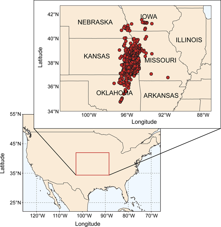
Figure 1. Location of sample sites. Map on lower left indicates Midcontinent region of North America that is the focus of our study (marked with box). Map on upper right shows in detail the area that is the source of our samples (including U.S. state boundaries). Dots on upper right map represent individual sample sites.
This relatively exceptional set of conditions provides an ideal setting to test for the presence or absence of community stability in a dynamic environmental setting (Holterhoff Reference Holterhoff1996; Olszewski and Patzkowsky Reference Olszewski and Patzkowsky2001a). Importantly, the duration of each cycle (approximately 400 kyr) is far less than the duration of the species that inhabited the basin (Holterhoff Reference Holterhoff1996), thus ensuring the metacommunity present was subject to repeated disruptions. While assessing paleocommunity structure at the level of stratigraphic beds at individual sites, or as close as possible to such a resolution, would be ideal, the limitations of our data make this impractical. Based upon the available data and given the limits of stratigraphic correlation across broad spatial regions, it was necessary to focus our study at the formation level. The formations considered from this particular region and time period do represent a constrained temporal unit for our study, given that individual taxa persist across multiple formations. Further, formations are lithostratigraphic units characterized by a predominant facies type and form only one part of a single major cyclothem, with cyclothems representing allostratigraphic units identified on the basis of their bounding discontinuities (Heckel Reference Heckel2013). This makes it possible for each formation to be assigned to a distinct environmental category based upon the predominant facies present in that formation (Heckel Reference Heckel2013; Fig. 2). It is also true, however, that numerous smaller-scale environmental transitions are occurring within the boundaries of any given formation that we have considered. Moreover, there are even hard to identify paraconformities within any formation for which environmental and paleoecological information is lacking. Thus, the results considered herein should only be treated as applying to and being commensurate with patterns examined at comparable temporal and spatial scales.
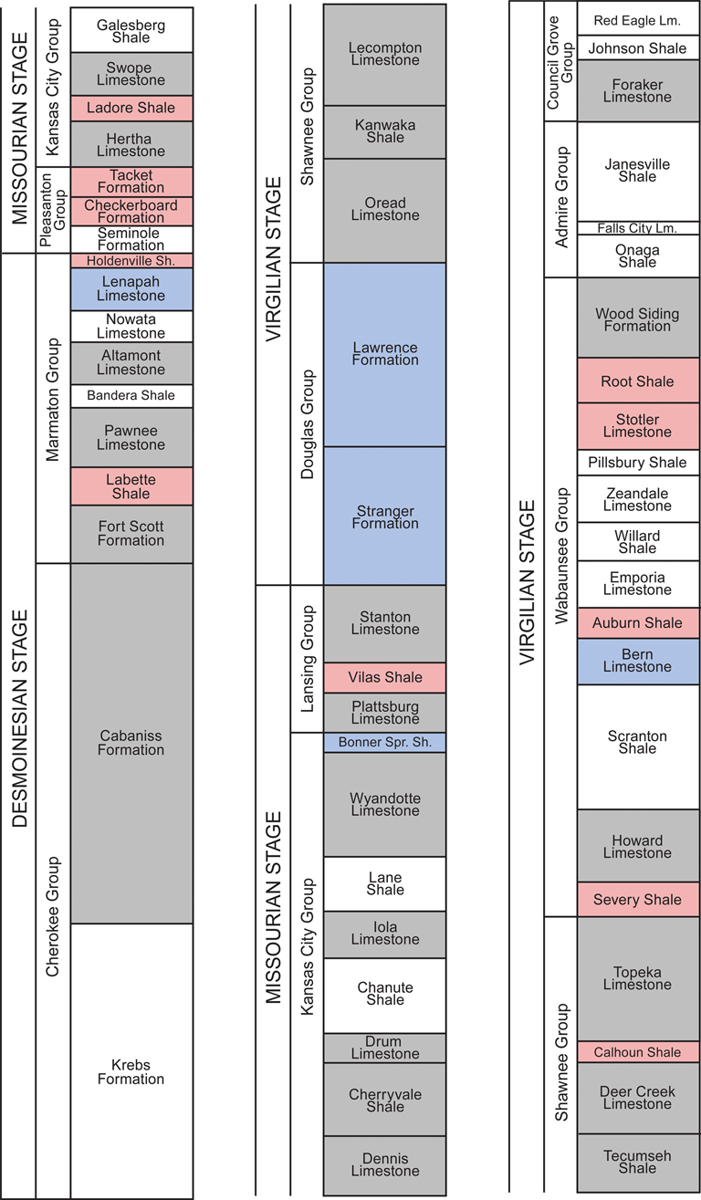
Figure 2. Middle and late Pennsylvanian (Desmoinesian to Virgilian) stratigraphy of the Midcontinent of the United States. Stratigraphic chart reads left to right, with the oldest formation on the bottom left and youngest formation on the top right. Colors indicate which environmental category each formation belongs to, as per Heckel (Reference Heckel, Fielding, Frank and Isbell2008, Reference Heckel2013). Red, sea-level lowstand phases (LP); blue, transitory phases (TP); and gray, sea-level highstand phases (HP). Formations in white are those where no or few brachiopods have been collected, usually because these formations are dominated by either marginal marine or terrestrial facies (Heckel Reference Heckel, Fielding, Frank and Isbell2008, Reference Heckel2013).
We use three environmental categories that parallel those previously proposed by Heckel (Reference Heckel, Fielding, Frank and Isbell2008, Reference Heckel2013) as part of his comprehensive paleoenvironmental study of this region. These are:
1. Sea-level highstand phases (HP)—characterized by condonot-rich black and gray phosphatic shales. These represent the peak of a marine transgression.
2. Transitory phases (TP)—characterized by limestone-dominated units deposited during the intermittent stages represented by either Heckel's (Reference Heckel, Fielding, Frank and Isbell2008, Reference Heckel2013) transgressive or regressive phases.
3. Sea-level lowstand phases (LP)—characterized by nearshore marine or terrestrial clastic sediments indicative of deltaic systems. These represent the peak of a marine regression.
It should be noted that these categories do not represent a single static environment, nor are they directly equivalent to a single ecological niche. Rather, they represent a broad set of environmental conditions that are strongly focused around changes in sea level. Sequence boundaries exist between LP and TP that are congruous with the temporal scale that is the focus of our study. Paleocommunities (constructed using the methods described in “Brachiopod Material”), were each assigned to one of these three categories, based upon their stratigraphic position and the paleoenvironmental interpretations of Heckel (Reference Heckel, Fielding, Frank and Isbell2008, Reference Heckel2013), to enable comparisons within and between environmental types.
Brachiopod Material
Our dataset consists of approximately 43,500 specimens of Pennsylvanian (Desmoinesian to Virgilian) articulated brachiopods from more than 1000 sample sites that today form a rough southwest/northeast transect across the Midcontinent Basin (Fig. 1, Supplementary Table 1). Specimen occurrences were sourced from the collections housed in the University of Kansas Biodiversity Institute, Division of Invertebrate Paleontology collections (KUMIP). Brachiopods were chosen for our study because they represent the dominant functional group in the Midcontinent Basin of North America and would have played a key role in nutrient cycling throughout the basin, both as suspension feeders removing particles from the water column and as a food source for durophagous predators.
As a significant proportion of the Pennsylvanian brachiopod specimens contained within the KUMIP collection have not yet been assigned to species, our study focuses on the generic diversity found within each paleocommunity. Brachiopods are an inherently ecologically conservative group (Rudwick Reference Rudwick1970), and thus little information is lost when utilizing brachiopod genera versus species. Numerous studies have previously demonstrated that generic diversity is adequate to assess ecological and paleoecological questions, particularly at the macroscale (e.g., Balmford et al. Reference Balmford, Lyon and Lang2000; Grelle Reference Grelle2002; Villasenor et al. Reference Villasenor, Ibarra-Manríquez, Meave and Ortiz2005; Clapham and Bottjer Reference Clapham and Bottjer2007).
Only specimens from sample sites that could be definitively assigned to a specific stratigraphic formation of relevant age were included in our analyses. Specimen occurrences were grouped by formation to create paleocommunities, with only paleocommunities of >50 specimens retained for analysis. Taxon occurrences and relative abundances for all formations are presented in Supplementary Table 2. The final dataset generated based upon these constraints consists of 38 discrete brachiopod paleocommunities that each represents a single temporal assemblage within the larger basin-wide fauna. Given the size and distribution of this dataset (both geographic and temporal), when compared with previous analyses of Paleozoic brachiopod paleoecology, it equals or exceeds in size and scale what has been previously used to consider patterns within paleocommunities, both in terms of richness and abundance.
Analyses
Methodological Framework
Comparison of community composition and/or diversity between samples lies at the core of the fields of ecology and conservation biology (Magurran and McGill Reference Magurran and McGill2011). As such, numerous methods and metrics exist to establish similarity or difference between samples (Santini et al. Reference Santini, Belmaker, Costello, Pereira, Rossberg, Schipper, Ceaușu, Dornelas, Hilbers and Hortal2017). Our approach to identifying community stability is based on determining whether the differences in diversity and composition among brachiopod paleocommunities could arise from equivalent assemblages being constituted from the same underlying sampling distribution. If so, any heterogeneities in diversity and taxonomic composition observed among paleocommunities would be no greater than expected from random sampling of a single assemblage. The general model to represent this would be:
 $$ \fleqalignno{{\rm Model\ }1 & = \lsqb {{\rm L}{\rm P}_1 = {\rm L}{\rm P}_2 = \ldots {\rm L}{\rm P}_i = {\rm T}{\rm P}_1 }= {\rm T}{\rm P}_2\cr & = \ldots {\rm T}{\rm P}_i = {\rm H}{\rm P}_1 = {\rm H}{\rm P}_2 = \ldots {\rm H}{\rm P}_i {{\rsqb}}&(1)} $$
where LP, TP, and HP correspond to the aforementioned environmental categories derived from the work of Heckel (Reference Heckel, Fielding, Frank and Isbell2008, Reference Heckel2013); the subscripts represent each paleocommunity; and increasing subscript values signify a decrease in paleocommunity age. If this model were corroborated, it would indicate no discernible statistical differences between any of the brachiopod paleocommunities. This would represent a profound form of coordinated stasis in which, regardless of bathymetric or environmental changes, the brachiopod fauna remained essentially unchanged.
If this model is not supported, we consider two alternate possibilities. First, it is possible that stability prevails within each environmental category but not across different environments. In this case, heterogeneity of paleocommunities from each environmental category would be no greater than would be expected from randomly sampling a single paleocommunity from that respective environment. However, heterogeneity between paleocommunities from different environmental categories would be statistically significant. The general model to represent this would be:
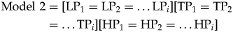 $$\fleqalignno{ \hbox{Model }2 &= \lsqb {\rm L}{\rm P}_1 = {\rm L}{\rm P}_2 = \ldots {\rm L}{\rm P}_i\rsqb \lsqb {\rm T}{\rm P}_1 = {\rm T}{\rm P}_2 \cr & = \ldots {\rm T}{\rm P}_i \rsqb \lsqb {{\rm H}{\rm P}_1 = {\rm H}{\rm P}_2 = \ldots {\rm H}{\rm P}_i} \rsqb &(2)}$$
This represents a more moderate form of paleocommunity stability, in which all paleocommunities that inhabit the same paleoenvironment can be considered to be homogeneous, perhaps as a result of some form of habitat filtering (Baldeck et al. Reference Baldeck, Harms, Yavitt, John, Turner, Valencia, Navarrete, Bunyavejchewin, Kiratiprayoon and Yaacob2013).
Finally, it is possible that no paleocommunity stability is manifest at all and that all paleocommunities are distinct from one another. The general model to represent this would be:
 $$ \fleqalignno{\hbox{Model }3 &= \lsqb {{\rm L}{\rm P}_1} \rsqb \lsqb {{\rm L}{\rm P}_2} \rsqb \ldots \lsqb {{\rm L}{\rm P}_i} \rsqb \lsqb {{\rm T}{\rm P}_1} \rsqb \lsqb {{\rm T}{\rm P}_2} \rsqb \ldots \cr &\quad \ \lsqb {{\rm T}{\rm P}_i} \rsqb \lsqb {{\rm H}{\rm P}_1} \rsqb \lsqb {{\rm H}{\rm P}_2} \rsqb \ldots \lsqb {{\rm H}{\rm P}_i} \rsqb &(3)}$$
This might arise because transgressive/regressive events associated with each cyclothem were disruptive enough to obliterate existing brachiopod paleocommunities and ensure that paleocommunities bore no resemblance to either the paleocommunity that had just been wiped out or to any other paleocommunity, previous or subsequent. Further, in this situation, it is likely that environmental forcing would be weak and historical paleocommunity composition would be extraneous, as each paleocommunity is formed anew after each environmental shift.
It would have, of course, been possible to consider many different scenarios beyond these three. With 38 different paleocommunities in our dataset, there are an astronomical number of possible models. Utilizing the vast majority of these models, however, would be capricious, as they clearly have no direct connection to established paleoecological theory. For example, it would be meaningless to assess whether every second LP paleocommunity most closely resembled every second HP paleocommunity, or whether paleocommunities that are assigned a prime number are homogeneous. Considering this vast universe of such potential models would also run counter to the goals of our study by obfuscating any potential connections that might exist between specific patterns in the structure of Pennsylvanian brachiopod paleocommunities and the range of ecological processes that we consider herein. The three models we have chosen to focus on represent scenarios that are both ecologically plausible and theoretically consistent and that also align with the approach employed in previous studies exploring the possibility of community stability.
We consider the probability of each of these scenarios using a combination of both multivariate statistics and likelihood-based model ranking methods. Employing multiple approaches allows us to best consider the different ways in which stability might be manifested and because it has been shown that patterns of relative stability or stasis can be obscured by sample size and choice of analytical method (Ivany et al. Reference Ivany, Brett, Wall, Wall and Handley2009).
Previous work to identify paleocommunity stability has generally focused on demonstrating either taxonomic stasis, wherein the majority of taxa persist over a protracted temporal interval, or ecological stasis, wherein taxonomic abundances and proportional representation of taxa remains unchanged (Ivany et al. Reference Ivany, Brett, Wall, Wall and Handley2009; Nagel-Myers et al. Reference Nagel-Myers, Dietl, Handley and Brett2013). The primary difference between these two concepts is that the latter includes both taxonomic information and abundance data. We explore the possibility of both taxonomic stasis and ecological stasis using presence data and taxon abundance data, respectively. Additionally, to determine whether community stability is manifest irrespective of taxonomic turnover, we also investigate for potential stability in community biodiversity (Chao et al. Reference Chao, Chiu and Jost2014).
It should be noted that it is conceivable that there are unspecified differences in preservation potential either of taxa and/or their abundances within each environmental category that could influence our attempt to consider patterns of stability and change in fossil brachiopod paleocommunities from the Pennsylvanian Midcontinent of North America. Although the scale of our dataset should account for this issue and the various analytical approaches we have chosen to employ also address sampling bias in different ways, the possibility of unspecified factors across each environmental category that we cannot assess but that might conceivably influence taxon presence/abundance is a potential caveat to our overall results.
For all analyses, brachiopod occurrences in each formation were first converted to relative abundances (Supplementary Table 2). If a dissimilarity measure was required, we used the Jaccard coefficient (Jaccard Reference Jaccard1912) when assessing presence data and the Bray-Curtis dissimilarity measure (Bray and Curtis Reference Bray and Curtis1957) to assess taxon abundance data. All analyses were carried out using R v. 3.6.1 (Ihaka and Gentleman Reference Ihaka and Gentleman1996).
Analyses of Taxonomic and Abundance Data
Potential dissimilarity between paleocommunities based upon taxonomic and relative abundance data was first visualized using principal coordinates analysis (PCoA), with relative abundance data additionally assessed using detrended correspondence analysis (DCA). To identify whether any differences in paleocommunity composition across the three environmental categories are significant (model 2), permutational multivariate analysis of variance (PERMANOVA), with 100,000 permutations and sampling interval as a fixed factor, was used.
We then directly evaluated all three of our scenarios (models 1–3) by applying the maximum-likelihood framework proposed by Handley et al. (Reference Handley, Sheets and Mitchell2009) to our relative abundance dataset. This approach is described in full in Handley et al. (Reference Handley, Sheets and Mitchell2009) and Nagel-Myers et al. (Reference Nagel-Myers, Dietl, Handley and Brett2013), and the interested reader is referred to those publications for a more detailed discussion of this method. In brief, this approach considers each paleocommunity to represent a multinominal observation and then determines which paleocommunities, if any, arise from the same underlying distribution by calculating the probability of observing all of the taxa present in that paleocommunity at the relative proportions at which they occur. Both Akaike's information criterion (AIC) and the Bayesian information criterion (BIC) were used to assess model fit.
Analyses of Biodiversity Data
Differences in biodiversity across the three environmental categories were assessed using diversity accumulation curves with associated rarefaction/extrapolation (Chao et al. Reference Chao, Chiu and Jost2014). The first three Hill numbers (see Chao et al. Reference Chao, Chiu and Jost2014) were used as measures of biodiversity. The first three Hill numbers are taxon richness (q = 0), the exponential of Shannon's entropy index (q = 1), and the inverse of Simpson's concentration index (q = 2). Extrapolation was undertaken up to 40,000 individuals. Pielou's evenness index (PEI; Pielou Reference Pielou1966) was used to measure assemblage evenness for each formation. High evenness reflects an assemblage in which a relatively equal numbers of individuals belong to each taxon, and low evenness indicates that only a small number of taxa make up the majority of the total abundance (Morris et al. Reference Morris, Caruso, Buscot, Fischer, Hancock, Maier, Meiners, Müller, Obermaier and Prati2014). Box-and-whisker plots based upon the Tukey method were generated using PEI results and a Kruskal-Wallis test (Kruskal and Wallis Reference Kruskal and Wallis1952) was used to identify whether significant differences in evenness exist between the three environmental categories.
Both Hill numbers and PEI results were further evaluated by using a likelihood-based framework focused on random-walk models that has previously been employed to identify and fit potential evolutionary models to compilations of ancestor–descendant trait variation (Hunt Reference Hunt2006; Hunt et al. Reference Hunt, Hopkins and Lidgard2015). In addition to evaluating if the model of best fit represents either a random walk or directional change, this approach also assesses for two varieties of stasis. The first, stasis, is defined as uncorrelated, normally distributed variation around a steady mean (Sheets and Mitchell Reference Sheets and Mitchell2001; Hunt et al. Reference Hunt, Hopkins and Lidgard2015). The second, strict stasis, represents instances in which the variance around the long-term mean is zero, such that there is no change between samples. To generate the necessary mean and variance values required to employ this likelihood-based approach, diversity data were bootstrapped (at 100, 1000 and 10,000 replicates) using the boot package in R (Canty Reference Canty2002). Bootstrapping was undertaken by resampling individual specimen identifications for each paleocommunity to create replicate versions of the relevant paleocommunity with potentially varying taxon abundances. One potential issue with this method is that results are possibly downward-biased, particularly in the case of taxon richness (q = 0), as the number of taxa in any one replicate cannot exceed the original sampled values. To assess how this issue may affect our result, for each formation, results of Hill number rarefaction (Chao et al. Reference Chao, Chiu and Jost2014) were used to determine the possible number of taxa that remain unsampled. The number of conceivable additional taxa stabilized at approximately 20,000 individuals for all formations, indicating that our extrapolation up to 40,000 individuals is more than sufficient to capture potential diversity. These additional taxa were then added to each paleocommunity to allow taxon richness to exceed the observed values (Supplementary Table 3). Abundance values for these hypothetical taxa were deemed to be equal to the observed taxon with the lowest abundance in the relevant formation, based upon the simplifying assumption that, given specimens of these hypothetical taxa were not recovered, their abundance must be equal to or less than all of the taxa actually observed. For both the observed and hypothetical datasets, AIC scores were used to assess model fit.
Results
Analyses of Taxonomic and Abundance Data Using PCoA and PERMANOVA
Results of ordination (PCoA and DCA) based upon relative abundance data show almost complete overlap for all three environments (Figs. 3A and 4), a result suggesting model 2 is unlikely to fit our data, as paleocommunities from each environment do not occupy distinct segments of ordination space. However, a definitive conclusion cannot be drawn based on ordination, given the first two axes of our PCoA explain only ≤34% of the total variance. Results of PERMANOVA comparing the three environmental categories and using relative abundance data fall close to the threshold required to demonstrate a statistically significant difference exists between categories (PERMANOVA: F = 1.517, p = 0.0513). Performing the same analysis with log-transformed abundance data finds no significant difference between categories (PERMANOVA: F = 1.4594, p = 0.0722). Because p > 0.05 for both untransformed and transformed relative abundance data, and given the results of PCoA and DCA, we reject the possibility of model 2 for relative abundance data. This result does not reject either model 1 or 3. When using only presence data, however, there is a significant difference between environmental categories (PERMANOVA: F = 1.9302, p = 0.0024), a result that supports model 2. Pairwise comparisons using the Bonferroni method for p-value correction indicate this is due to a significant difference between HP and LP paleocommunities (HP vs. LP: p = 0.003), and PCoA results based upon presence data demonstrate a similar pattern (Fig. 3B).
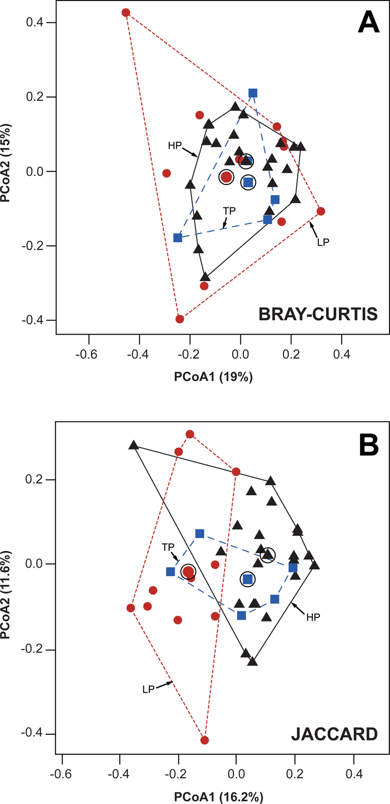
Figure 3. Principal coordinates analysis (PCoA) biplot for Pennsylvanian brachiopod paleocommunities from the North American Midcontinent. A, PCoA based upon relative abundance data and using the Bray-Curtis dissimilarity measure. B, PCoA based upon presence data and using the Jaccard similarity coefficient. Symbols represent individual paleocommunities. Circles (red), sea-level lowstand phases (LP); squares (blue), transitory phases (TP); and triangles (black), sea-level highstand phases (HP). Convex hulls outline each of the three environmental categories used in our study. Symbols inside open circles mark the centroid of each convex hull.

Figure 4. Detrended correspondence analysis (DCA) biplot for Pennsylvanian brachiopod paleocommunities from the North American Midcontinent. Symbols represent individual paleocommunities. Circles (red), sea-level lowstand phases (LP); squares (blue), transitory phases (TP); and triangles (black), sea-level highstand phases (HP). Convex hulls outline each of the three environmental categories used in our study.
This disparity between results based upon relative abundance data versus those based upon presence data can be attributed to the larger number of rare taxa present in HP paleocommunities. Thirty-one taxa that occur in HP paleocommunities are never found in LP paleocommunities, and the vast majority of these 31 taxa occur at extremely low abundances (Supplementary Table 2). Taxa that occur at high relative abundances in HP paleocommunities, however, are also present in LP paleocommunities, and vice versa, thus leading to no significant difference between these two environmental categories when relative abundance data are considered.
Analyses of Abundance Data Using AIC and BIC
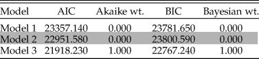
A somewhat different picture emerges based upon maximum-likelihood analyses of these data. Maximum-likelihood estimates based upon relative abundance data provide 100% support for model 3, as indicated by Akaike and Bayesian weights (Table 1). While AIC can favor more complex models, given both AIC and BIC equally support model 3, this result is unlikely to be due to overfitting (Nagel-Myers et al. Reference Nagel-Myers, Dietl, Handley and Brett2013). This indicates a continually changing relative abundance structure, such that each paleocommunity is considered to be distinct from any other, an unsurprising result, given that individual taxon abundances vary through time and within environmental categories (Supplementary Table 2). The high variance in taxon abundance is such that designating what constitutes a “dominant” taxon remains a somewhat open question. Some taxa certainly always remain rare, but many taxa that are “common” in some formations are extremely rare in others. We also do not see evidence for abundant taxa tracking preferred environments (Bonuso et al. Reference Bonuso, Newton, Brower and Ivany2002a), with taxon abundance also highly variable within the same environmental category. Thus, these results indicate there is no evidence for stability in paleocommunities either through time or across environments.
Table 1. Rankings for model fit to changes in paleocommunity taxon abundances. Each model is described in detail in the “Analyses” section. For each model, the Akaike information criterion (AIC), Akaike weight, Bayesian information criterion (BIC), and Bayesian weight are provided. Values are rounded to three decimal places.
Analyses of Biodiversity Data
Absolute taxonomic richness is highest in HP paleocommunities, which contain 66 of the 69 taxa in our dataset (Fig. 5). Diversity accumulation curve confidence intervals are non-overlapping between HP and LP samples for both q = 0 and q = 2. For a fixed sample size, where confidence intervals for Hill number rarefaction/extrapolation do not overlap, significant difference (at a level of p < 0.05) is guaranteed (Chao et al. Reference Chao, Chiu and Jost2014). Values for q = 0 are sensitive to the number of rare taxa, q = 1 values are sensitive to both rare and abundant taxa, and q = 2 values are sensitive to only abundant taxa (Chao et al. Reference Chao, Chiu and Jost2014). The patterns observed for each Hill number therefore indicate that HP assemblages contain larger numbers of rare taxa when compared with TP and, particularly, LP assemblages. PEI values show a similar result (Fig. 6), with lower evenness in HP paleocommunities reflective of the higher number of rare taxa, but there is no significant difference between evenness for the three environmental categories (Kruskal-Wallis chi-squared = 5.43776, p = 0.065949).
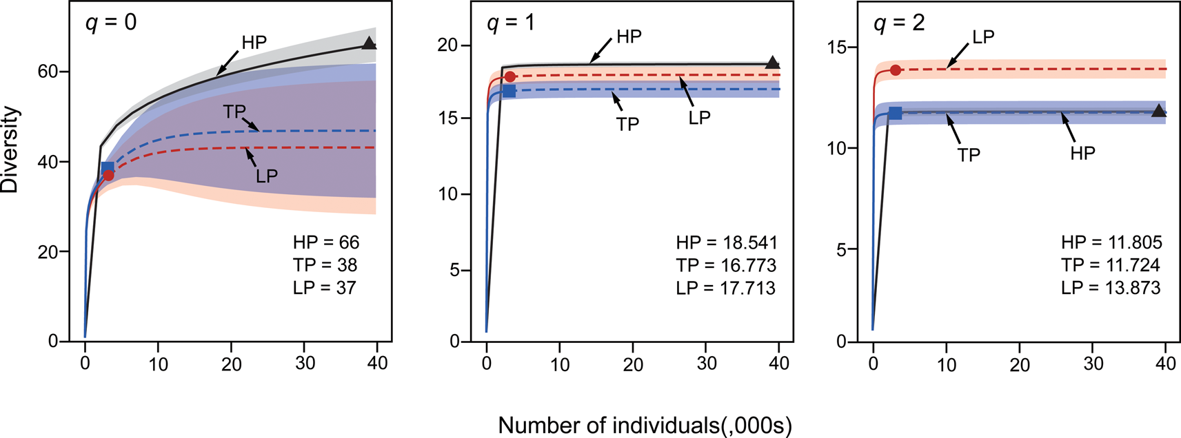
Figure 5. Sample-size-based rarefaction (solid line) and extrapolation (dashed lines) for Pennsylvanian brachiopod diversity. Hill number q = 0 (left panel), q = 1 (middle panel), and q = 2 (right panel). Red, sea-level lowstand phases (LP); blue, transitory phases (TP); and black, sea-level highstand phases (HP). Reference sample for each sampling interval is indicated by a solid symbol (LP, circle; TP, square; HP, triangle). Shaded areas represent confidence intervals for each environmental category. Overall Hill number values for each environmental category are listed in the bottom right corner of each plot.

Figure 6. Box plots of Pielou's evenness index scores for each environmental category. Dark band inside box = median. Whiskers = ±1.5*interquartile range (IQR). Solid circle represents sample site that falls outside the range of whiskers. The lower whisker for the transitory environmental category is equal to the lower bound of the IQR for that category.
Assessment of diversity values using likelihood-based estimates identify stasis as the best-supported model for the entire metacommunity, which includes all paleocommunities combined (Table 2, Fig. 7). Based upon AIC scores, for all diversity indices, there is greater than 99% support for overall stasis (but not strict stasis). This means diversity values do fluctuate but remain normally distributed around a mean value. Raising or lowering the number of bootstrap replicates results in no appreciable difference in Akaike weights and no change in which model is best supported (Supplementary Table 4). AIC scores for our hypothetical dataset containing additional potential taxa also identify stasis as the best-supported model (Supplementary Table 4). Analysis of PEI values using the same methods yields the same result obtained for Hill numbers (Table 2; Supplementary Table 4).
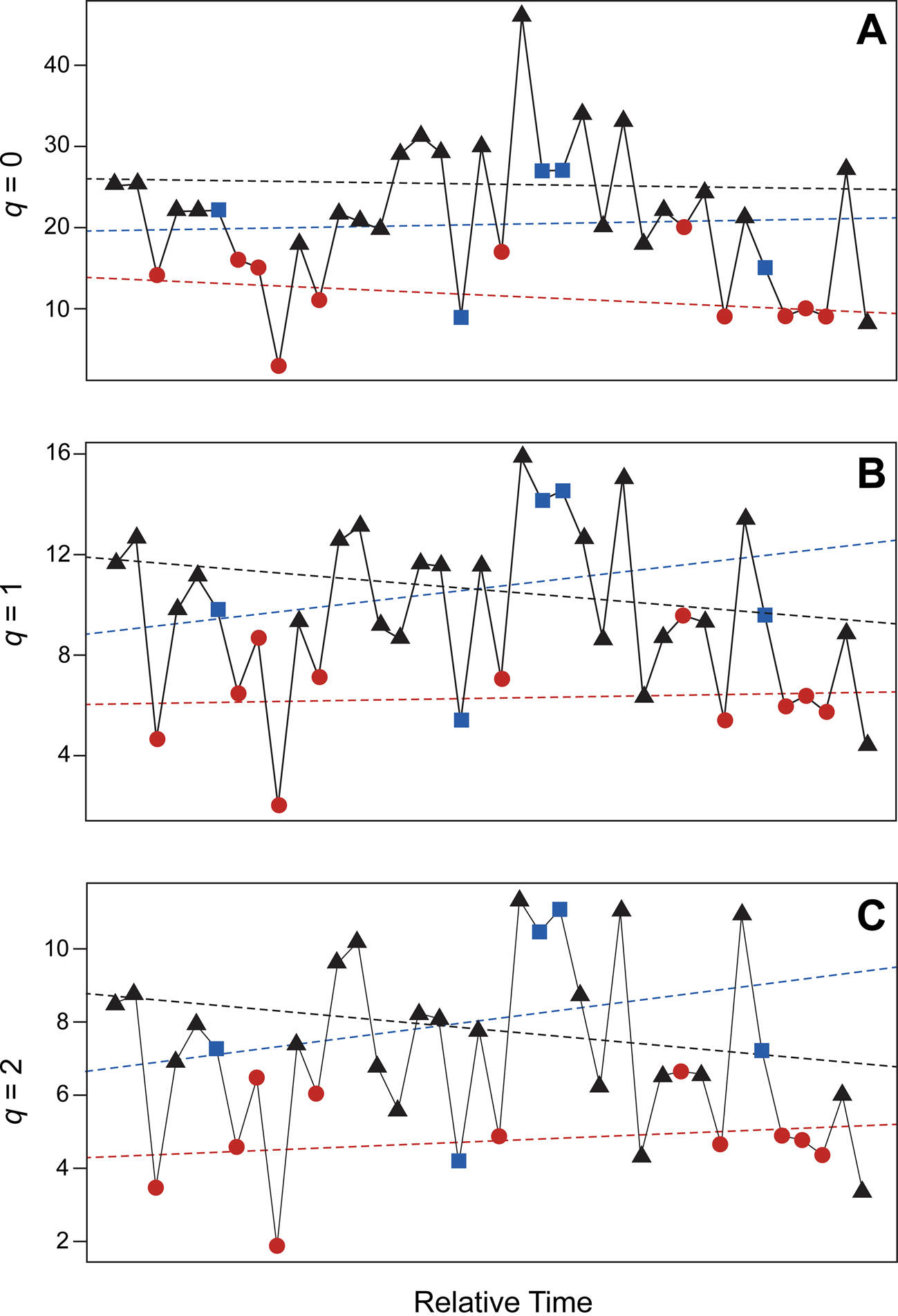
Figure 7. Diversity values for Pennsylvanian brachiopod paleocommunities of the North American Midcontinent. A, Taxon richness (q = 0); B, exponential of Shannon's entropy index (q = 1); C, inverse of Simpson's concentration index (q = 2). Circles (red), sea-level lowstand phases (LP); squares (blue), transitory phases (TP); and triangles (black), sea-level highstand phases (HP). Dashed lines represent linear line of best fit for each diversity index and environmental category (as indicated). For all indices, stasis is the best-fitting model.
Table 2. Maximum-likelihood parameter estimates for diversity values. AICc values (AICc = sample-size adjusted AIC values) and Akaike weights are listed for four models: GRW (general random walk), URW (unbiased random walk), Stasis, and S. Stasis (strict stasis). Definitions for each of these four models are discussed in the “Analyses” section. Taxon richness, Shannon's entropy, and inverse Simpson's represent the first three Hill numbers respectively (q = 0–2). Values are rounded to three decimal places. For all indices, stasis is the best-fitting model, with greater than 99% support.

Discussion
Our results highlight the importance of considering multiple approaches when evaluating the possibility of community stability in the fossil record, as different approaches may yield divergent results. For instance, multivariate analyses based on relative abundance data reject the possibility of a distinct and discernible paleocommunity associated with each environmental category, suggesting paradoxically that either stasis prevails through time and across environments (model 1) or that no paleocommunity stability is manifest at all (model 3). Yet multivariate analysis of presence data suggests a moderate form of stasis, wherein paleocommunities are homogenous within environmental categories but heterogeneous between categories (model 2). A maximum likelihood–based assessment of relative abundance data, however, provides unequivocal support for repeated turnover (model 3), refuting the possibility of paleocommunity stasis. Finally, if the precise taxonomic identity of representatives of any paleocommunity are not considered, and instead diversity is the focus, stasis (model 1) is the returned result. This incongruence between our various results, while seemingly problematic, reflects the varying methods we employ to assess for stability at different positions on the ecological hierarchy (sensu Jørgensen and Nielsen Reference Jørgensen and Nielsen2013) and that conceivably distinct processes may drive the patterns observed at each scale.
At the scale of individual brachiopod paleocommunities, it is evident that abiotic change is an important driver of paleocommunity structure and that paleocommunity turnover is linked to each phase of major transgressive/regressive events. Importantly, the composition and underlying abundance distribution of any new paleocommunity may or may not resemble the paleocommunity that was present during a previous phase, even when that phase is representative of the same environmental category. Therefore, the net pattern does not resemble that of a Markov process, in that the structure of a paleocommunity is not dependent upon the composition of the previous paleocommunity. Instead, each paleocommunity seemingly is formed via the luck of the draw and/or the exigencies of recruitment or survival. This lack of stability suggests that there is no obvious evidence for habitat tracking (Brett and Baird Reference Brett, Baird, Erwin and Anstey1995; Olszewski and Patzkowsky Reference Olszewski and Patzkowsky2001a) at the scale observed, as brachiopod paleocommunities with consistent taxonomic compositions do not re-emerge in subsequent formations in association with shifts in environment. An absence of habitat tracking partially conflicts with previous work on Midcontinent paleocommunities, which identified both habitat tracking and de novo paleocommunity formation (Holterhoff Reference Holterhoff1996; Olszewski and Patzkowsky Reference Olszewski and Patzkowsky2001a). However, this previous work focused on alternate taxa and a narrower temporal and geographic scale, which may account for the differing result.
Given that our study focuses on a relatively broad geographic region and temporal interval, it is not possible to discern whether changes in taxonomic composition were also happening at a scale below the level of assemblages within formations. Because our paleocommunities represent a metacommunity concept that incorporates significant time averaging, it is logical to assume that some amount of taxonomic turnover is also happening at smaller spatial and temporal scales. Analyzing such change would be both important and valuable but at present is not possible, given the stratigraphic resolution of our data. Thus, it is important to reiterate that the pattern of de novo paleocommunity formation we uncover is documented at the level of paleocommunities sensu Bennington and Bambach (Reference Bennington and Bambach1996), and considering smaller spatial and temporal intervals could lead to additional or alternate conclusions. However, it is also important to recognize that thanks to the detailed sedimentological and stratigraphic perspective available for the region (e.g., Heckel Reference Heckel, Fielding, Frank and Isbell2008, Reference Heckel2013), it is clear that different formations connote substantially different paleoenvironmental conditions and the scale of environmental change that occurs between formations far exceeds the environmental fluctuations that occur within any one formation. At its most extreme, the boundary between formations represents a sequence boundary (Heckel Reference Heckel, Fielding, Frank and Isbell2008): an erosional surface representative of subaerial exposure and a time of maximum environmental perturbation. The scale of environmental change between formations is such that significant biological turnover is most likely greater during the transition from one formation to the next than within any one formation. Undoubtedly, important environmental changes do occur within formations, and consideration of the fluctuations in community structure that may be associated with these changes could help further expand the notion of why it is important to consider the nature of stability and change in ecological assemblages at several hierarchical levels, but at the present time and in this study system, this is not possible.
Despite the taxonomic constituents of paleocommunities being highly variable, there seem to be limits on taxon richness for each paleoenvironmental category (Fig. 7, Supplementary Table 2). This implies rules for taxon packing in the Pennsylvanian brachiopod paleocommunities of the Midcontinent. Consistent patterns of taxon packing in communities have been posited in several classic treatises in ecology (e.g., MacArthur and Wilson Reference MacArthur and Wilson1967; Hubbell Reference Hubbell2001). In the specific case of our brachiopod paleocommunities, differences in taxon richness between paleoenvironmental categories may reflect limitations on the available substrate needed for individual brachiopod larva to successfully develop into adults (Fürsich and Hurst Reference Fürsich and Hurst1974; Bonuso and Bottjer Reference Bonuso and Bottjer2006; Topper et al. Reference Topper, Strotz, Holmer and Caron2015). Once available physical space is exhausted, there could be exclusion based upon incumbency (Valentine et al. Reference Valentine, Jablonski, Krug and Roy2008), with the upper limit on the number of taxa present in any one paleocommunity correlated with available habitat. The quantity of available habitat would expand with increasing water depth (Olszewski and Patzkowsky Reference Olszewski and Patzkowsky2003), as a greater part of the shelf-slope becomes available for occupation. Energy budgets and associated per capita metabolic activity may also contribute to the observed pattern. Metabolic activity in any one community/paleocommunity has been demonstrated to exhibit remarkable stability, despite species turnover and environmental disruption (Finnegan et al. Reference Finnegan, McClain, Kosnik and Payne2011; Strotz et al. Reference Strotz, Saupe, Kimmig and Lieberman2018a). This stability can be achieved through limits on maximum species richness, exclusion of copious taxa with higher metabolic demands, limits on taxon abundance, or some combination of all three (Strotz et al. Reference Strotz, Saupe, Kimmig and Lieberman2018a). The limits on taxon packing we identify in the Pennsylvanian Midcontinent may thus also reflect physiological controls that limit how many species can be maintained in any single community, with distinct environments able to sustain a differing number of species due to differences in energy availability (Glazier Reference Glazier1987; Strotz et al. Reference Strotz, Saupe, Kimmig and Lieberman2018a).
An even more profound pattern of paleocommunity stability emerges when the fauna is assessed in its totality, with all diversity metrics exhibiting stasis for the entire study interval (Table 2, Fig. 7). This suggests γ-diversity, defined as the total species diversity in a landscape (Whittaker Reference Whittaker1960; Whittaker et al. Reference Whittaker, Willis and Field2001), remains unchanged. Perhaps this is to be expected, given there is no evidence of either extinction or speciation in the regional biota (Olszewski and Patzkowsky Reference Olszewski and Patzkowsky2001a). Thus, when populations of a species disappear locally due to environmental and/or physical disruption, they still can possibly reappear in one or more subsequent paleocommunities. Moreover, any environmental changes are invariably reversed in a subsequent cyclothem. The minimal impact on γ-diversity may reflect the presence of ample refugia (Stewart et al. Reference Stewart, Lister, Barnes and Dalén2010), allowing taxa to persist in the face of environmental change.
When considered together, these patterns of paleocommunity structure provide the necessary evidence to reconstruct the macroecological dynamics in Pennsylvanian brachiopod faunas from the Midcontinent Basin of North America. As sea level rises, newly available habitat is randomly seeded by migrating taxa in the form of essentially arbitrary pulls from the greater pool of γ-diversity. Ultimately α-diversity, represented in our study by the total taxon richness in any one paleocommunity, becomes saturated once the carrying capacity of the relevant paleoenvironment is reached, and any taxa that subsequently attempt to join the paleocommunity are excluded. This somewhat resembles “environmental selection,” as proposed by Bambach (Reference Bambach1994) and also parallels the mechanisms for recruitment as implemented in the theory of island biogeography (MacArthur and Wilson Reference MacArthur and Wilson1963, Reference MacArthur and Wilson1967), although operating at a much larger scale. Taxa that successfully colonize may have intrinsic advantages such as increased dispersal capacity or greater fecundity (Clark and Ji Reference Clark and Ji1995), but fluctuations in rank abundance (Supplementary Table 2) suggest stochastic processes, such as vagaries in recruitment dynamics and fluctuations in the import of biotic interactions (Miller Reference Miller1986) may be just as important, at least in the long-term realm of these paleocommunities. Once a regression event begins, paleocommunity turnover recommences. As the regressive phase progresses, taxa may persist due to higher levels of abundance, because their niche more closely corresponds to current conditions, or because they simply have not yet been culled. At sea-level lowstand, α-diversity again stabilizes until such time as a transgressive phase commences and turnover begins anew.
With each cyclothem, this pattern of diversity ramp-up and drawdown is repeated, resulting in no net ecological change over time. As γ-diversity remains unaffected, this cycle can potentially persist over very long periods of time (Buzas and Culver Reference Buzas and Culver1994). This pattern can be usefully viewed in the context of Hubbell's (Reference Hubbell2001) unified neutral theory of biodiversity and biogeography, in which γ-diversity can be considered equivalent to Hubbell's (Reference Hubbell2001) metacommunity, representing a stable pool of potential immigrants that can seed local communities as suitable niche space is created (Rosindell et al. Reference Rosindell, Hubbell and Etienne2011). In this context, random taxa from the metacommunity form new paleocommunities that “replace” the paleocommunity that was previously present. Individual paleocommunities are thus essentially neutral, with their diversity fixed by the carrying capacity of the paleoenvironment. In our case, however, we are proposing repeated wholesale community replacement, a rather more drastic scenario than the attritional replacement of individuals within local communities proposed by Hubbell's unified neutral theory (Hubbell Reference Hubbell2001; Rosindell et al. Reference Rosindell, Hubbell and Etienne2011).
The pattern of stability in the face of constant change we identify is potentially analogous to results from modern marine communities as they recover from disruptive events over much shorter timescales. For example, foraminifera communities subjected to disruption by tropical cyclones rapidly re-established previous species distribution patterns, with no loss of biodiversity, once the cyclone passed (Strotz et al. Reference Strotz, Mamo and Dominey-Howes2016). Evidence indicates, however, that these communities never reach steady state and exist in a permanent state of intermediate recovery (Strotz et al. Reference Strotz, Mamo and Dominey-Howes2016). Similar patterns have been observed for coral communities (Richards et al. Reference Richards, Beger, Pinca and Wallace2008) and fish communities (Planes et al. Reference Planes, Galzin, Bablet and Sale2005) that were removed from parts of Pacific atolls multiple times by the nuclear testing programs of the late twentieth century. Given these events are on much shorter timescales than those experienced by the paleocommunities we assess, it is not clear whether they represent similar phenomena, such that a direct connection exists between the various ecological scales, or instead are merely analogous and fundamentally distinct, and thereby driven by different sets of ecological processes (see discussion of ecological hierarchies in Valentine Reference Valentine1970; Eldredge and Salthe Reference Eldredge and Salthe1984; Eldredge Reference Eldredge1986). Considering this issue of scale is necessary in any paleoecological investigation for a variety of reasons, including because paleocommunities are not directly analogous to biological communities (Bennington and Bambach Reference Bennington and Bambach1996). In particular, while the constituent taxa of a paleocommunity may occupy the same geographic space, they may not be continually coterminous in time and thus may not have interacted ecologically. Yet, just as fossil species differ from the extant biological populations that are the purview of biology but still represent a unit of biological import (Strotz and Allen Reference Strotz and Allen2013), so paleocommunities still represent a cohesive ecological unit that connects hierarchically to extant communities (Pandolfi Reference Pandolfi2002; DiMichele et al. Reference DiMichele, Behrensmeyer, Olszewski, Labandeira, Pandolfi, Wing and Bobe2004).
The stability in γ-diversity through time we observe aligns with the concept of coordinated stasis, concurring with both initial definitions and subsequent works (e.g., Brett and Baird Reference Brett, Baird, Erwin and Anstey1995; Morris et al. Reference Morris, Ivany, Schopf and Brett1995; Bonuso et al. Reference Bonuso, Newton, Brower and Ivany2002a,Reference Bonuso, Newton, Brower and Ivanyb; Ivany et al. Reference Ivany, Brett, Wall, Wall and Handley2009). However, we cannot identify the “stasis packages” that according to Brett et al. (Reference Brett, Ivany and Schopf1996) are the benchmark of “true” coordinated stasis. This is because, even though a large proportion of the Pennsylvanian Midcontinent brachiopod taxa persist through time, they do not cohere into continuous paleocommunities or biofacies (sensu Boucot Reference Boucot1975; Brett and Baird Reference Brett, Baird, Erwin and Anstey1995; Morris et al. Reference Morris, Ivany, Schopf and Brett1995). Thus, the detailed ecological stasis typical of coordinated stasis is lacking. Further, and associated with this, we did not find evidence for ecological locking (Morris et al. Reference Morris, Ivany, Schopf and Brett1995), a potential causal mechanism for coordinated stasis, as taxonomic composition does not persist through environmental shifts and taxon abundance is highly variable. While γ-diversity does persist, it is a metaconcept that combines multiple paleocommunities, and thus the interaction that is a key element of ecological locking is difficult to identify. This lack of evidence for coordinated stasis or ecological locking, in comparison to archetypal studies on both these concepts centering on the Hamilton Group of New York State (Brett and Baird Reference Brett, Baird, Erwin and Anstey1995; Morris et al. Reference Morris, Ivany, Schopf and Brett1995), may possibly be at least partly attributed to differences in temporal and spatial scale between our study and previous work on the Hamilton Group, as well as key differences in the tectonic setting of the Hamilton Group versus the Pennsylvanian Midcontinent (Brett and Baird Reference Brett, Baird, Erwin and Anstey1995; Heckel Reference Heckel2013). It is also judicious that we consider our results in the context of the important topic that Bennington and Bambach (Reference Bennington and Bambach1996) addressed: whether recognizing paleocommunity stability through time entails that the same individual paleocommunities (with individuals defined sensu Hull [1976]) persisted over long intervals of time, or instead only generally similar ones persisted. Given the absence of evidence for persistent biofacies and ecological locking, the brachiopod paleocommunities in the Pennsylvanian Midcontinent that we considered seem to be representatives of classes (Hull Reference Hull1976; Wiley Reference Wiley1978); they resemble one another but were not single, historically connected individuals.
The repeated cycle of turnover at the formation level we identify also parallels aspects of the turnover pulse hypothesis (Vrba Reference Vrba1985, Reference Vrba1993), wherein changes in the composition of paleocommunities are initiated by changes in the physical environment. Without environmental shifts of significant magnitude, changes in a paleocommunity are nondirectional around a mean configuration. This is because, although unremitting biotic interactions can generate shifts in fitness at the population level, as per a qualified definition of the Red Queen hypothesis (Strotz et al. Reference Strotz, Simoes, Girard, Breitkreuz, Kimmig and Lieberman2018b), because these shifts do not affect all populations equally, they appear as stasis at the level of species in communities. Only a more complete transformation of the physical environment can lead to assemblage turnover. However, over longer timescales and at higher scales of the ecological hierarchy (e.g., γ-diversity), we observe stasis. This may partly be explained by considering the sloshing bucket hypothesis (Eldredge Reference Eldredge, Crutchfield and Schuster2003, Reference Eldredge2008). This hypothesis posits that disruptions can result in community breakdown but may not be sufficient to lead to full ecosystem collapse. As long as the relevant threshold of disruption is never reached, continued paleocommunity reconstitution after each episode of environmental change is highly likely. In the particular case considered herein, there are two end-member paleocommunities (HP and LP) that are repeatedly able to re-form because the environmental disruption experienced by the greater γ-species pool is never enough to cause its complete ecological breakdown. It is not possible, though, to identify the threshold at which community collapse is likely assured, that is, what causes the bucket to get kicked over. This is because we are only considering a time interval that represents part of a stable faunal package (Brett and Baird Reference Brett, Baird, Erwin and Anstey1995; Morris et al. Reference Morris, Ivany, Schopf and Brett1995; Brett et al. Reference Brett, Ivany and Schopf1996; Olszewski and Patzkowsky Reference Olszewski and Patzkowsky2001b).
Miller (Reference Miller1986) proposed the concept of “community replacement” for patterns of community turnover identified in the fossil record. Shifts in the environmental regime are the primary driver of community replacement, leading to wholesale changes in species-abundance distributions. Importantly, Miller (Reference Miller1986) proposed that community replacement occupied a higher hierarchical level than ecological changes driven by biotic interactions and that, given the time frames involved, paleoecologists need to carefully consider the hierarchical scale being observed. Pandolfi (Reference Pandolfi2002) also argued that the hierarchical scale being considered has a marked effect on how ecological dynamics in fossil assemblages are interpreted, and our results reiterate this important contention. In particular, in some respects, paleocommunity stasis can be hard to discern when it is assessed via patterns of species association and relative abundance. However, when it comes to patterns of diversity, paleocommunity stability can be manifest even where taxonomic turnover is evident. It would thus seem that, when it comes to identifying stability in community structure through time, sometimes the names don't matter but the numbers do.
Conclusions
In this study we closely examine the Carboniferous brachiopod paleocommunities from the Midcontinent of North America to determine whether paleocommunity structure can remain stable despite recurring shifts in environmental setting. We show that marked shifts in both taxonomic composition and the associated abundance of taxa provide little evidence for obdurate ecological stasis at the level of paleocommunities. However, close examination of diversity patterns identifies stability exists at what constitutes a different ecological scale, as per Eldredge's (Reference Eldredge, Crutchfield and Schuster2003) sloshing bucket hypothesis. This suggests that rules operating at higher levels in the ecological hierarchy may allow for ecological stability even in the face of constant disequilibrium. Based on these results, we advocate for careful consideration of hierarchical scale when interpreting the ecological dynamics of fossil assemblages.
Acknowledgments
We thank N. López Carranza and R. LaVine for comments on an earlier version of this manuscript and J. Kimmig for assistance with collections-related matters. We would also like to thank W. Kiessling in his role as editor for Paleobiology, along with M. Clapham and two anonymous reviewers for their comments and suggestions that helped to improve the final version of our paper. Financial support for this project was provided by NSF EF 1206757 and DBI 1602067. This material is based upon work (by B.S.L.) supported while working at the National Science Foundation.


 Open access