

Introduction
Geographic ranges of species are fundamental units of biogeography. The properties associated with geographic ranges, including their structure, organization, size, and location, are controlled by a suite of factors such as organismal biology, life history, niche breadth, dispersal ability, phylogenetic affinity, and historical environmental changes (Willis Reference Willis1922; Anderson Reference Anderson1984a,Reference Andersonb; Brown et al. Reference Brown, Stevens and Kaufman1996; Gaston and Spicer Reference Gaston and Spicer2001; Huntley et al. Reference Huntley, Collingham, Green, Hilton, Rahbek and Willis2006; Gaston Reference Gaston2008; Gaston and Fuller Reference Gaston and Fuller2009). The specific properties of ranges have been shown to affect both micro- and macroevolutionary processes, including the potential for speciation (Cardillo et al. Reference Cardillo, Huxtable and Bromham2003; Goldberg et al. Reference Goldberg, Lancaster and Rhee2011) and extinction (Payne and Finnegan Reference Payne and Finnegan2007; Harnik et al. Reference Harnik, Simpson and Payne2012; Runge et al. Reference Runge, Tulloch, Hammill, Possingham and Fuller2015; Saupe et al. Reference Saupe, Qiao, Hendricks, Portell, Hunter, Soberon and Lieberman2015).
The relationship between geographic range size and extinction risk has garnered increased attention lately with the recognition that global ecosystems are in rapid decline and are showing signs of incipient ecosystem collapse analogous to the “Big 5” mass extinction events in the geological past (Barnosky et al. Reference Barnosky, Matzke, Tomiya, Wogan, Swartz, Quental, Marshall, McGuire, Lindsey, Maguire, Mersey and Ferrer2011; Hull et al. 2015). Taxonomic groups as disparate as plants, insects, mammals, amphibians, birds, reptiles, and mollusks have all shown dynamic changes in the size, shape, and location of individual species’ ranges in response to global change, on timescales ranging from tens to thousands of years (Parmesan et al. Reference Parmesan, Ryrholm, Stefanescu, Hill, Thomas, Descimon, Huntley, Kaila, Kullberg, Tammaru, Tennent, Thomas and Warren1999; Lyons Reference Lyons2003; Walther et al. Reference Walther, Post, Convey, Menzel, Parmesan, Beebee, Fromentin, Hoegh-Goldberg and Bairlein2002; Chen et al. Reference Chen, Hill, Ohlemuller, Roy and Thomas2011; Botts et al. Reference Botts, Erasmus and Alexander2013). Consequently, ecologists are increasingly looking to the fossil record as a source of historical data pertaining to how geographic range size and location can be affected during mass extinction events, and to how aspects of geographic range confer either resilience or vulnerability to extinction. This has produced a wealth of studies that use fossil data to study the relationship between geographic range size and extinction risk (e.g., Payne and Finnegan Reference Payne and Finnegan2007; Saupe et al. Reference Saupe, Qiao, Hendricks, Portell, Hunter, Soberon and Lieberman2015) as part of a larger attempt to build predictive models for the future (Hadly et al. Reference Hadly, Spaeth and Li2009; Raia et al. Reference Raia, Passaro, Fulgione and Carotenuto2012; Hull and Darroch Reference Hull and Darroch2013; Darroch and Wagner Reference Darroch and Wagner2015; Finnegan et al. Reference Finnegan, Anderson, Harnik, Simpson, Tittensor, Byrnes, Finkel, Lindberg, Liow, Lockwood, Lotze, McClain, McGuire, O-Dea and Pandolfi2015; Saupe et al. Reference Saupe, Qiao, Hendricks, Portell, Hunter, Soberon and Lieberman2015). Despite these efforts, little is currently known regarding whether geographic range size (and range-size dynamics) can be reconstructed accurately from fossil locality data, and which commonly used paleoecological methods for range reconstruction are the most reliable (though see recent work on correcting biases in occupancy metrics; Foote Reference Foote2016). A systematic methodology for quantifying the accuracy of these methods under different extinction-related and biogeographic scenarios will allow us to effectively calibrate the quality of the spatial fossil record in specific time intervals, and to place future paleobiogeographic studies on a firm conceptual footing.
Fossil species aside, defining and measuring the geographic ranges of modern species is itself problematic. Maps or other characterizations present much-simplified versions of the complex spatial and temporal patterns in which individual organisms are dispersed (Brown et al. Reference Brown, Stevens and Kaufman1996). Ranges are most frequently mapped as irregular areas (“outline maps”) that encompass all localities where a species has recently (or historically) been recorded (Brown et al. Reference Brown, Stevens and Kaufman1996). Some authors have, for example, distinguished between the “extent of occurrence” (the absolute limits of the occurrence of a species) and the “area of occupancy” (the area over which a species can be found at any one time). The latter will almost always be smaller than the former, because species do not occupy all areas within their range (Gaston Reference Gaston2003), and it suffers from issues of spatial scale. That is, a positive relationship exists between the area of occupancy identified for a species and the scale of the analysis (see International Union for Conservation of Nature and Natural Resources [IUCN 2015] Red List document “Categories and Criteria”). Consequently, area of occupancy may be an unsuitable attribute to reconstruct from fossil data, and all discussions and data herein focus on extent of occurrence.
In this study, we use simulation studies to test whether fossil point (i.e., locality) data can be used to reconstruct range sizes and range dynamics. Specifically, we test (1) the degree to which typical paleobiological methods for range-size reconstruction reliably detect decreases in geographic range size, and (2) whether these methods accurately determine extinction selectivity based on the presumption that narrowly distributed species go extinct more readily (e.g., Finnegan et al. Reference Finnegan, Heim, Peters and Fischer2012; Saupe et al. Reference Saupe, Qiao, Hendricks, Portell, Hunter, Soberon and Lieberman2015). We aim to identify the most reliable methods for range-size reconstruction and to pinpoint critical thresholds in the number of sites required for such methods to consistently produce biologically meaningful results.
Although the distribution and areas of fossiliferous sediments have undoubtedly changed through time, performing these experiments under a best-case scenario (i.e., assuming no loss of surface sediments) is a fundamental first step before additional layers of complexity are applied. We suggest these methods can be modified to be relevant to older time periods, and will thus enable more accurate studies of macroevolutionary and macroecological patterns and processes throughout Earth history.
Methods
Reduction in Geographic Range Size
Reduction in a species’ range size is often used as an indicator of extinction risk (e.g., Payne and Finnegan Reference Payne and Finnegan2007; Harnik et al. Reference Harnik, Simpson and Payne2012; Runge et al. Reference Runge, Tulloch, Hammill, Possingham and Fuller2015; Darroch and Wagner Reference Darroch and Wagner2015; Hull et al. 2015; IUCN 2015; Saupe et al. Reference Saupe, Qiao, Hendricks, Portell, Hunter, Soberon and Lieberman2015). To address our question of whether paleobiological methods for range-size reconstruction can detect decreases in geographic range size, we used terrestrial range-size data reflecting “extent of occurrence” for extant herpetological species (taken from the IUCN Red List [IUCN 2015]). Large and small range sizes were chosen from similar geographic regions to represent pre- and post-range-contraction stages, respectively. Given the possible strong control exerted by the distribution of preservable areas on the accuracy of range-size reconstructions, we expected the performance of range-size reconstruction methods to differ between wet and dry biomes, with the former expected to preserve fossil material more readily and completely across space. We therefore performed two sets of simulations to compare range-size dynamics in both biomes.
For the “wet” biome simulations, we used two closely related snake species native to the central and southeastern United States—Nerodia fasciata (banded water snake) and Nerodia cyclopion (green water snake). Nerodia fasciata has a relatively large range (851,850.2 km2), while N. cyclopion has a relatively small range (263,278.5 km2) that is largely a subset of the range of N. fasciata (Fig. 1); we therefore treat N. fasciata as our pre-impact range and N. cyclopion as our post-impact range, representing an approximately 70% reduction in range size.

Figure 1 Mapped ranges (in white) for species used in the range-size contraction simulations, with wet ranges (N. fasciata and N. cyclopion) on the left and dry ranges (U. scoparia and A. canorus) on the right. The preservable parts of each range (taken from the USGS National Hydrography Dataset) are superimposed in black. Hypothetical “pre-extinction” and “post-extinction” ranges are shown in top and bottom panels, respectively.
For the “dry” biome simulations, we used two (unrelated) species with ranges centered in the western United States—Uma scoparia (Mohave fringe-toed lizard) and Anaxyrus canorus (Yosemite toad). Although these ranges are nonoverlapping, they are geographically proximal and possess equivalently small preservable areas, providing a good test for identifying range contraction in relatively arid environments. Of these two species, U. scoparia has the larger range (39,199.64 km2) and represents the pre-impact stage, whereas A. canorus has a smaller range (10,315.37 km2) and represents the post-impact stage, an approximately 74% reduction in range size. In both wet and dry biome simulations, our “post-extinction” ranges are reduced in size but are not fragmented; fragmentation is an additional process that may affect threatened species but is not specifically examined here (Fahrig Reference Fahrig2003).
We populated these species’ ranges with randomly placed fossil sites and employed standard paleobiological methods for range-size reconstruction to assess how consistently these methods retrieved a significant size difference between the two ranges (discussed later). By varying the number of sites in each simulation, we also tested the number of sites required to reliably recognize range-size contraction. Importantly, however, constraints were placed on where the fossil occurrences were populated. That is to say, not all areas within the geographic ranges of terrestrial species have equal preservation potential; most of the time, an organism needs to land in a depositional environment (i.e., a setting where sediment is accumulating) to stand any chance of being preserved. These depositional environments are typically aquatic in nature, including streams, rivers, and lakes (e.g., Behrensmeyer Reference Behrensmeyer1991). Thus, to ensure realism in the simulations, we approximated the “preservable” portions of each species’ geographic range using the 1:24,000 scale U.S. Geological Survey (USGS) Waterbodies Dataset (see Figs. 2, 3), which forms part of the National Hydrography Dataset (USGS 2017). We extracted all surface water features (lakes, ponds, streams, and rivers) from within each species’ geographic range and randomly placed occurrences only within these water bodies.
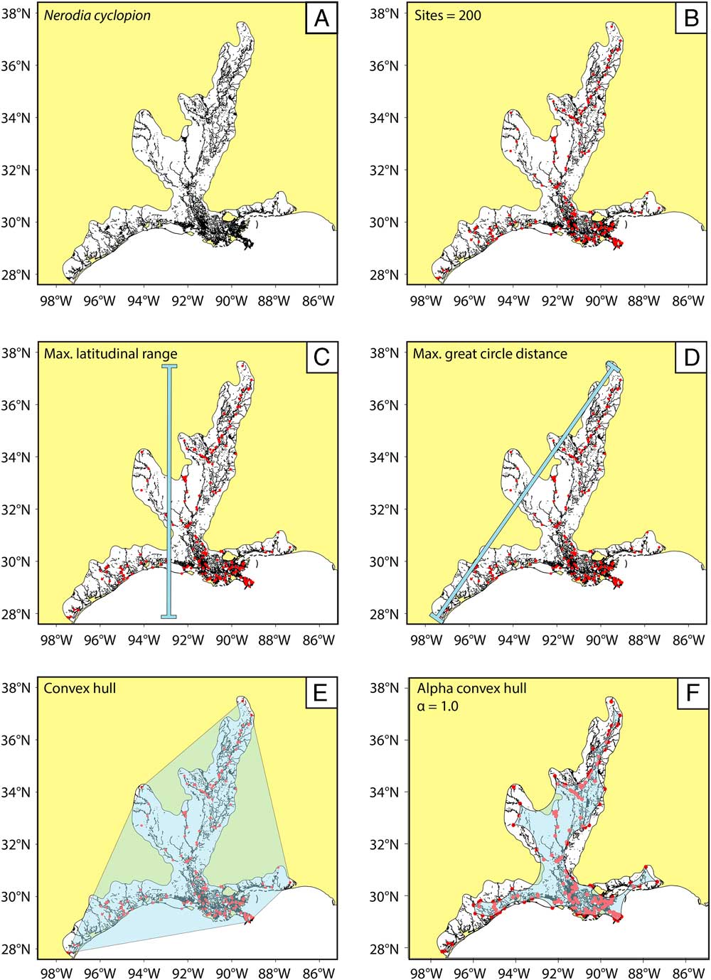
Figure 2 Methodology for range-size simulations and reconstruction; example using N. cyclopion. A, The preservable parts of each range (in black) are extracted from the mapped range taken from the IUCN Red List (in white). B, n fossil sites are randomly (and iteratively) placed within the preservable part of the range. C–F, The simulated range is then calculated (overlain in light blue) using our four methods for paleo range reconstruction; note that convex-hull methods are prone to overestimating the actual range, whereas alpha-hull methods tend to produce underestimates.
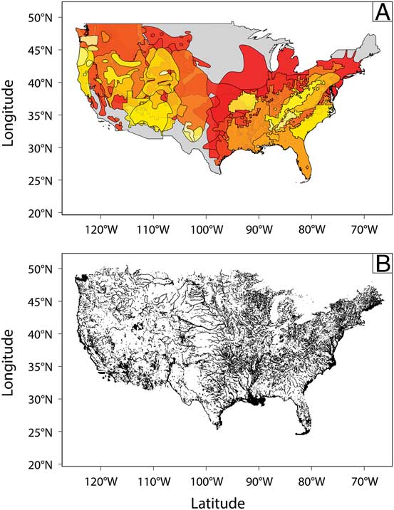
Figure 3 (A) The distribution of extant ranges (taken from the IUCN Red List) used for extinction-modeling studies, with larger ranges shown in red colors and smaller ranges in yellow colors (for full list of species, see Supplementary Table 2). (B) Distribution of areas in North America likely to preserve a paleontological record, defined as surface water features and depositional environments (part of the USGS National Hydrography Dataset). Note the inhomogeneous distribution of preservable areas, and thus the preservable parts of species ranges, across the continent.
We ran simulations using four paleobiological methods for geographic range-size reconstruction: maximum latitudinal range, maximum great-circle distance between fossil occurrences, convex hull, and alpha convex hull (see Fig. 2). Of these, maximum latitudinal range (Finnegan et al. Reference Finnegan, Heim, Peters and Fischer2012; Foote and Miller Reference Foote and Miller2013), maximum great-circle distance (Jablonski Reference Jablonski1987; Jablonski and Roy Reference Jablonski and Roy2003; Foote and Miller Reference Foote and Miller2013; Foote et al. Reference Foote, Ritterbush and Miller2016), and convex hull (Stigall and Lieberman Reference Stigall and Lieberman2006; Hendricks et al. Reference Hendricks, Lieberman and Stigall2008; Myers and Lieberman Reference Myers and Lieberman2010; Raia et al. Reference Raia, Passaro, Fulgione and Carotenuto2012; Desantis et al. Reference Desantis, Tracy, Koontz, Roseberry and Velasco2012; Darroch et al. Reference Darroch, Webb, Longrich and Belmaker2014; Darroch and Wagner Reference Darroch and Wagner2015; Saupe et al. Reference Saupe, Qiao, Hendricks, Portell, Hunter, Soberon and Lieberman2015) have been used extensively by previous workers to measure extent of occurrence, whereas alpha hull has not.
Alpha hulls are constructed of polygons (“alpha shapes”) composed of piecewise linear simple curves that are concave with respect to the range. This method is able to capture range holes and invaginations at the margins of ranges, and is therefore potentially less prone to overestimation errors than convex-hull methods. Alpha convex hulls are parameterized by the term “α,” which dictates the concavity of the resulting alpha shape; for consistency, we use an α value of 1.0, although we explore the effect of varying this parameter (see Supplementary Fig. 1).
We iteratively ran simulations using site numbers ranging from 3 (i.e., the minimum required for convex-hull calculation) to 200, which approximates the range of locality numbers that typically characterize fossil tetrapods. Alpha hulls were problematic when using fewer than 25 sites (i.e., would tend to produce unrealistic geometries that could not be projected into geographic coordinates) and were thus not calculated for fewer than this number. For statistical power, we performed 100 iterations for each species using each method.
We quantified the accuracy and consistency of range-reconstruction methods in two ways. First, we used one-way Mann-Whitney U tests to assess whether range-reconstruction methods reliably identified post-impact ranges as smaller than pre-impact ranges. Second, we measured the extent to which simulations capture the absolute percentage range contraction in both wet (~70% contraction) and dry (~74% contraction) biomes.
Extinction Scenarios
Previous research suggests species with small geographic ranges preferentially go extinct relative to those with large range sizes (Purvis et al. Reference Purvis, Gittleman, Cowlishaw and Mace2000; Jones et al. Reference Jones, Purvis and Gittleman2003; Kiessling and Aberhan Reference Kiessling and Aberhan2007; Payne and Finnegan Reference Payne and Finnegan2007; Harnik et al. Reference Harnik, Simpson and Payne2012; Finnegan et al. Reference Finnegan, Heim, Peters and Fischer2012; Saupe et al. Reference Saupe, Qiao, Hendricks, Portell, Hunter, Soberon and Lieberman2015). To address our question of the degree to which paleo range-size reconstruction methods accurately determine extinction selectivity, we selected 40 North American species from the IUCN Red List to represent the distribution of a hypothetical pre-extinction clade. Under normal (i.e., relatively static) environmental conditions, organisms within a clade or taxonomic group typically display an approximately log-normal distribution of range sizes (see, e.g., Anderson Reference Anderson1977, Reference Anderson1985; Gaston Reference Gaston1996, Reference Gaston1998). As such, we chose species with an eye toward creating such a distribution (Fig. 3). Species were also chosen so as to exhibit minimum geographic bias in the sizes of ranges and the latitudinal/longitudinal range of centroids; the result is a collection of species with small and large ranges that are evenly distributed across North America (Supplementary Fig. 2). The identities of these species and details of habitat/ecology are given in Supplementary Table 1. As with the simulations on range-size reduction detailed earlier, we extracted the preservable (i.e., aquatic) parts of each range using the USGS Waterbodies Dataset (USGS 2017).
Using this distribution of species, we set arbitrary range size “extinction thresholds”: these are minimum range sizes below which we expect species to go extinct in a hypothetical extinction scenario. Species with ranges larger than the identified threshold were deemed “survivors,” whereas those below the threshold were considered “victims.” We considered both a “low-sensitivity” threshold and a “high-sensitivity” threshold, designated by natural breaks in the range-size frequency distribution (see Supplementary Fig. 3); our low-sensitivity thresholds involved relatively large differences in range size between victims and survivors, whereas our high-sensitivity thresholds involved smaller differences. These thresholds correspond to extinction intensities of 85–90% and 45–52% for low- and high-sensitivity thresholds, respectively. To mirror the stochastic nature of extinction dynamics, we added noise to the extinction selectivity signal, such that a few large-ranged species went extinct, and not all small-ranged species went extinct (see Supplementary Table 2). Because we used three measures of range size (absolute area, maximum latitudinal range, and maximum great-circle distance) that have different distributions of relative sizes, we set three different extinction thresholds.
Range-size simulations were implemented to examine the extent to which our range-reconstruction methods accurately predicted the distribution of survivors and victims in each extinction scenario. Similar to our range –contraction simulations, we reconstructed species’ range sizes using varying numbers of occurrences, and for statistical power, we performed 100 iterations for each species, method, and number of sites, resulting in a total of 168,000 simulations.
We assessed the number of simulations that correctly predicted extinction selectivity using binary logistic regressions. We log-transformed all range-size data to conform to the assumption of linearity of the independent variables and the log odds. We counted a simulation as successful if it returned a significant p-value (α level 0.05) in the binary logistic analysis, indicating it found signal in the data suggesting that the smaller-ranged species go extinct more readily.
All range-size simulations and statistical analyses were performed using the R programming language (R Development Core Team 2015) and the following packages: ‘sp’ (Pebesma and Bivand Reference Pebesma and Bivand2005), ‘maptools’ (Lewin-Koh et al. Reference Lewin-Koh, Bivand, Pebesma, Archer, Baddeley, Bibiko, Dray, Forrest, Friendly, Giraudoux, Golicher, Rubio, Hausmann, Hufthammer, Jagger, Luque, MacQueen, Niccolai, Short, Stabler and Turner.2011), ‘PBSmapping’ (Schnute et al. Reference Schnute, Boers, Haigh and Couture-Beil2008), ‘rgeos’ (Bivand and Rundel Reference Bivand and Rundel2013), ‘rgdal’ (Bivand et al. Reference Bivand, Keitt and Rowlingson2014), and ‘alphahull’ (Pateiro-Lopez and Rodruiguez-Casal Reference Pateiro-Lopez and Rodruiguez-Casal2009).
Results
Reduction in Geographic Range Size
All four range-reconstruction methods reliably recognized the range-size decrease in the dry biome experiments (U. scoparia and A. canorus; Fig. 4; Supplementary Fig. 4). All simulations returned significant size decreases using only 3 sites with maximum great-circle distance, maximum latitudinal range, and convex-hull methods. That is to say, no overlap occurred in range-size estimates between the two species across all simulations. When using the alpha-hull method, all simulations correctly identified size decreases at the lowest number of sites (i.e., 25). Mann-Whitney U tests confirm these results, wherein simulated post-impact ranges were statistically smaller at 95% confidence for all methods and site numbers. Iterative subsampling of simulated ranges (Supplementary Fig. 5) confirms these general patterns.
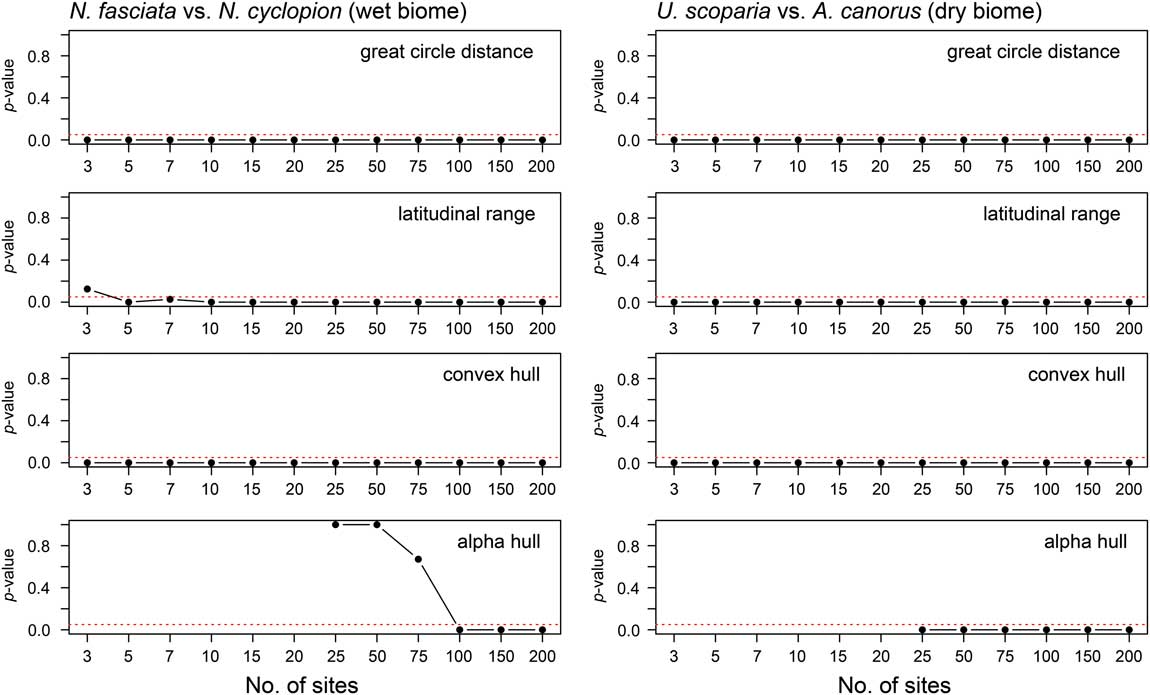
Figure 4 The p-values from Mann-Whitney U tests comparing pre- and post-contraction ranges in both wet and dry biomes. Values below the 95% confidence interval (p=0.05; marked by dashed line in each plot) indicate that the distribution of simulated post-contraction ranges is statistically smaller than that of pre-contraction ranges.
The performance of range-reconstruction methods differed for the wet biome (N. fasciata and N. cyclopion). Maximum great-circle distance and convex-hull methods returned a significant reduction in range size using 3 sites, whereas maximum latitudinal range required 5. In contrast, alpha hull incorrectly identified pre- and post-impact range sizes using 25 to 75 sites, such that it reconstructed N. fasciata as the smaller ranged of the two species (see Supplementary Fig. 4). On average, pre-impact ranges were significantly greater than those of post-impact ranges for all site numbers and reconstruction methods aside from alpha hull; Mann-Whitney U analyses suggested 100+ sites are required for the alpha-hull method to recognize accurately a decrease in range size.
The results from our range-contraction simulations can be summarized as follows: (1) Range-size reconstruction methods differ in their performance between wet and dry biomes with regard to correctly identifying a range contraction. In the wet biome, maximum great-circle distance and convex-hull methods perform best (especially when limited to <5 sites), whereas maximum latitudinal range and alpha hull perform well only when 5+ and 100+ sites are used, respectively. (2) Range-reconstruction methods more reliably identify range-size contractions in dry rather than wet biomes. (3) Maximum great-circle distance and convex-hull methods identify range-size contractions more reliably than maximum latitudinal range and alpha-hull methods.
Extinction Scenarios
We quantified performance of the four range-reconstruction methods in estimating extinction risk using binary logistic regressions. Since we performed 100 simulations for each site number, we tabulated the number of simulations that correctly predicted the distribution of survivors and victims among our 40 species (Fig. 5). The performance of the range-reconstruction methods differed significantly between low- and high-sensitivity thresholds (~90% and ~50% species extinction, respectively); however, at the high-sensitivity threshold, three of the methods (maximum latitudinal range, maximum great-circle distance, and convex hull) predict extinction patterns at relatively low numbers (~10) of sites (>90% of p-values≤0.05). Of these, the convex-hull method performed best, predicting extinction risk in 98% of simulations when using only 5 sites to reconstruct range sizes. Maximum great-circle distance also performed well, with 80 and 96% of simulations correctly predicting extinction risk using only 5 and 7 sites, respectively. In contrast, alpha hull performed poorly, with a success rate of only 5% using 25 sites.
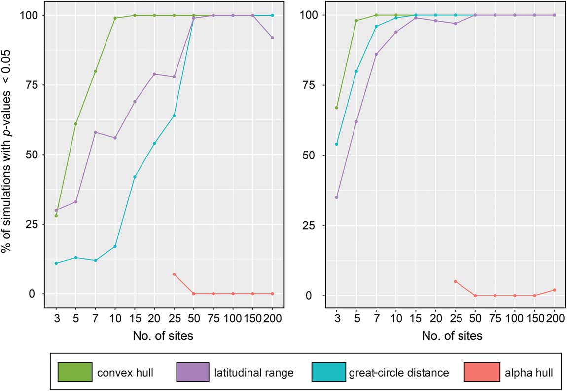
Figure 5 Performance of range-size reconstruction methods at recovering the correct distribution of extinct and surviving taxa in extinction-modeling studies, expressed as percentage of total simulations. Left plot illustrates our low-sensitivity scenario; right plot shows the high-sensitivity scenario. Note the improvement of many methods when a larger number of simulated fossil localities is used.
Interestingly, all four methods performed worse under the low-sensitivity (~90% extinction) threshold. The relative ordering of the methods in terms of their performance remained almost unchanged from the results under the high-sensitivity (~50% extinction) threshold, but the number of sites required to attain a high level of accuracy increased. For example, for maximum latitudinal range, the number of sites rose from 10 to 50 for >90% of simulations to correctly predict extinction risk; likewise, for maximum great-circle distance, the number of sites required to achieve the same accuracy rose from 7 to 50.
Discussion
Best and Worst Methods for Range Reconstruction
Results from both the range-contraction and extinction simulations suggest macroevolutionary and macroecological patterns, at least in the relatively recent past, can be studied reliably using only a few fossil occurrence sites. Range contraction in both dry and wet biomes can be preserved and detected using a variety of commonly used paleobiological methods. Within the wet biome, we find that great-circle distance and convex-hull methods perform best and give statistically consistent results using only 3+ sites. Latitudinal range also performs well above a threshold of 5+ sites, whereas alpha hull performs relatively poorly, requiring a threshold of 100+ sites.
We find that range contraction is easier to detect in dry biomes than in wet biomes, with three sites sufficient for all four methods. This result at first appears counterintuitive: more preservable area should logically produce a more reliable fossil record, and thus a more reconstructable range. However, when comparing the sizes of the two ranges, the patchiness of the preservable areas in the dry biome may allow for detection of a statistical difference between the larger and smaller range (although this may hold only when fossil “localities” are randomly distributed, as they are here). We make a preliminary attempt to test this hypothesis by sampling 0.5° by 0.5° grid cells from within each of the four ranges shown in Figure 1 (see Supplementary Figs. 6, 7), and comparing mean pairwise distances between the centroids of preservable areas within each grid cell. The results, however, reveal that mean distances are equivalent in both wet and dry biomes (see Supplementary Fig. 8), and thus patchiness in preservable areas may not be driving the observed pattern and some other explanation may be required.
Similar to the range-contraction experiments, our extinction simulations offer justification for many paleoecological and macroevolutionary studies that reconstruct paleo-range sizes and dynamics; three of the four studied range-reconstruction methods (maximum great-circle distance, maximum latitudinal range, and convex hull) accurately predicted (>90% of p-values ≤ 0.05) patterns of species’ survival based on range size using only approximately 10 fossil sites in our high-sensitivity scenario. Although there were substantial differences between the low- and high-sensitivity scenarios, the results suggest site thresholds that could potentially guide future studies. That is to say, to achieve at least 90% accuracy assuming a low-sensitivity threshold, 10+ sites are needed for the convex-hull method, and 50+ sites are needed for maximum latitudinal range and maximum great-circle distance. Alpha hulls performed extremely poorly in both scenarios (see Supplementary Table 3). Although the method can perform well when sites are randomly placed anywhere within the range (e.g., see Supplementary Fig. 1), alpha shapes struggle to resolve real range geometries when clustered within linearly-oriented features such as streams, rivers, and lakes. Increasing the α value for hulls can help to reconstruct more realistic geometries, but the resulting polygons become less concave and thus equivalent to convex-hull methods.
Perhaps counterintuitively, all range-reconstruction methods performed better under the high-sensitivity (~50% extinction) scenario over the low-sensitivity (~90% extinction) scenario. One explanation for this may be a lack of statistical power, creating difficulty in recovering the correct extinction pattern under the low-sensitivity threshold. That is to say, few species “survive” in this scenario, making it difficult for the model to determine correctly the difference in range size between those species that go extinct and those that do not. Alternatively (or in addition), the better method performance in the high-sensitivity scenario may be an inadvertent result of the specific species that straddle the low- and high-sensitivity thresholds. At the low-sensitivity threshold, the methods are attempting to recover the “survival” of western species with ranges centered in more arid regions and the “extinction” of smaller-ranged species with ranges centered primarily in Florida and Louisiana. Given the limited distribution of water bodies (and therefore of preservable area) in the western United States, all methods will consistently underestimate range size of the western-distributed species. Conversely, the preservable parts of each range will more closely approximate the perimeter of species distributed in the wetter southeastern United States, and thus a random placement of sites will more closely reconstruct actual range sizes for these species. In other words, the simulations are trying to recover a result wherein a species prone to range underestimation survives and a species prone to range overestimation goes extinct. Although this arrangement of species and thresholds was entirely inadvertent, it illustrates the difficulty of determining the relative sizes of species’ ranges from fossil locality data if these species are distributed in radically different biomes.
Practical Comparisons with the Terrestrial Fossil Record
The number of localities needed for accurate paleo range-size analyses can be compared directly with the number available for various taxa in the fossil record. Such quantification provides a broad sense for how useful the fossil record is as a spatial, rather than a temporal, data set. Given that our range simulations are most applicable to terrestrial (non-volant) vertebrates, we downloaded all Cenozoic tetrapod (mammals, reptiles, and amphibians) occurrence data from the Paleobiology Database (https://paleobiodb.org; details given in Supplementary Material 1). We split occurrences by North American Land Mammal Ages (NALMAs); these time bins range in duration from 226,000 years (Rancholabrean: ~0.24–0.014 Ma) to 10.2 Myr (Arikareean: 30.8–20.6 Ma) and are probably among the shortest intervals for which multispecies range-size or biogeographic analyses could be undertaken on continental scales (see, e.g., Fraser et al. Reference Fraser, Hassall, Gorelick and Rybczynski2014). Because many paleobiogeographic analyses of terrestrial faunas have been performed at the genus rather than the species level (see, e.g., Hadly et al. Reference Hadly, Spaeth and Li2009), we calculated the number of occurrences for both genera and species. The results (Fig. 6) illustrate the percentage of species and genera within NALMAs preserved at each number of sites treated in our simulations (details for individual NALMAs given in Supplementary Fig. 9).

Figure 6 Percentage of Cenozoic fossil terrestrial tetrapod (mammal, reptile, and amphibian) species (left) and genera (right) discovered in increasing numbers of fossil sites (defined as localities with unique paleolatitude and paleolongitude coordinates) in North America. Boxes illustrate the spread of values for all North American Land Mammal Ages (NALMAs), with mean values superimposed as points (see Supplementary Fig. 6 for details of individual NALMAs). Comparing these values with the trajectory of percentage successful simulations for different range-reconstruction methods shown in Figs. 4 and 5 provides a measure of the utility of the spatial fossil record of tetrapods for analysis of range-size dynamics in deep time.
At the species level, results range from poor coverage (only 10% of species in the Rancholabrean are preserved at 3 sites, decreasing to nearly 0% for 5+ sites) to remarkably good coverage (e.g., 30% of species are preserved at 5 sites and ~10% of species are preserved at 20 sites in the Wasatchian). For the vast majority of NALMAs (with the exception of the Monroecreekian and Duchesnian), between 10% and 50% of species are preserved at 3+ sites, a number that our simulations suggest is sufficient for detecting changes in range-size dynamics using great-circle distance and convex-hull methods in either wet or dry biomes. At 10+ sites (the threshold suggested for two of our methods for detecting the correct split of victims and survivors in our extinction experiment), most time bins possess between 1% to 10% of species (and ~17% in the Wasatchian), which still represents an encouraging return when 100–300 species are typically recorded in each time bin. Only in the Wasatchian are any species (0.23%) preserved at 100+ sites, rendering alpha hull effectively useless for this type of analysis. The results are even more encouraging at the genus level, with 11 out of 22 NALMAs possessing 30–40% of genera represented at 5+ sites. Cumulatively, these percentages suggest that many hundreds of Cenozoic species may be sufficiently well sampled to examine changes in their distribution and geographic range size and to test a broad swath of macroecological and macroevolutionary questions. Logically, these percentages will only increase if coarser time resolution is allowed (see, e.g., Desantis et al. Reference Desantis, Tracy, Koontz, Roseberry and Velasco2012; Darroch et al. Reference Darroch, Webb, Longrich and Belmaker2014), although the macroecological and environmental hypotheses invoked to explain any discovered patterns will also be correspondingly broader.
Caveats and Future Directions
Our methodological framework for these simulations makes a number of assumptions, all of which introduce significant caveats to the conclusions we reach concerning the utility and completeness of the spatial fossil record. One major assumption concerns our random placement of simulated fossil sites within ranges. In reality, fossil sites are aggregated and “patchy” on all scales (Plotnick Reference Plotnick2017), which may have a significant effect on the accuracy of range reconstruction. The other assumptions we make can be organized loosely into “top-down” (climate and tectonic activity) versus “bottom-up” (necrolysis, biostratinomy, and diagenesis) effects that control the quality of the vertebrate fossil record (Noto Reference Noto2010). With regard to the former, although we accounted for differential preservation and incompleteness of the fossil record by varying site numbers and by restricting occurrences to preservable areas, our most influential assumption is that the entirety of a species’ range is preserved and able to be interrogated by paleontologists. However, weathering, erosion, tectonism, and isostatic/eustatic sea-level change are responsible for constantly removing or burying large quantities of fossil-bearing sedimentary rocks, such that the exposed rock area for any given geological unit typically decreases as you go further back in Earth history (Raup Reference Raup1976; note, however, this pattern is likely more apparent for terrestrial than marine sediments, see, e.g., Peters and Heim Reference Peters and Heim2010). Consequently, it seems likely that the accuracy of many range-size reconstruction methods will covary with the surface expression of fossiliferous sediments through time.
In terms of bottom-up effects, another assumption inherent in these simulations is that all species are equally abundant (and thus equally likely to be found as fossils) and have equivalent taphonomic potentials. With regard to the first point (rarity), the relative abundance of a species may have a huge impact on the likelihood of it being discovered as a fossil. Many authors have argued that the preservation of any one species is potentially subject to an “abundance threshold,” such that rare taxa are less likely to be preserved (and/or subsequently discovered) than common species. Modern mammalian species exhibit a bimodal pattern of rarity, with an overabundance of species in both the rarest and most common categories (Yu and Dobson Reference Yu and Dobson2000); a large proportion of fossil tetrapod species may therefore be underrepresented in the fossil record.
With regard to the second point (taphonomy), a suite of taphonomic processes favors the preservation of some taxa over others. The most obvious of these is size—the bones of animals under 100 kg tend to weather beyond recognition more rapidly than those of larger animals (Behrensmeyer Reference Behrensmeyer1978; Janis et al. Reference Janis, Scott and Jacobs1998; Plotnick et al. Reference Plotnick, Smith and Lyons2016). Thus, in general, smaller species may require more atypical environmental conditions to be reliably preserved and, correspondingly, may tend to have smaller reconstructed ranges. In addition to overall body size, the robustness of skeletal elements (Behrensmeyer et al. Reference Behrensmeyer, Stayton and Chapman2003, Reference Behrensmeyer, Fursich, Gastaldo, Kidwell, Kosnik, Kowalewski, Plotnick, Rogers and Alroy2005), selective scavenging (Bickart Reference Bickart1984; Livingston Reference Livingston1989), and ambient environmental energy at the time of deposition (i.e., a lake margin vs. a fast-flowing river; Kidwell and Flessa Reference Kidwell and Flessa1996) are all processes that favor the preservation of some species over others, and almost certainly exert a taphonomic overprint on the reconstructed ranges of terrestrial species. With that said, the USGS Waterbodies Dataset likely represents a minimum estimate for the distribution of preservable area within a species’ range. Although tetrapod remains are most often fossilized in streams, rivers, and lakes, they can also be preserved in paleosols, aeolian sands, and within overbank deposits, none of which are incorporated here. Caves and karsted environments in particular make up a significant fraction of fossil sites in the Quarternary (Jass and George Reference Jass and George2010; Plotnick et al. Reference Plotnick, Kenig and Scott2015; although see Noto Reference Noto2010 for a comprehensive list of preservable terrestrial subenvironments). Our modeled preservable area should thus be seen as conservative, and the accuracy of range-size reconstructions may be considerably better than indicated by our simulations (especially in arid environments).
Another potential problem with reconstructing range sizes from fossil locality data involves the issue of postmortem transport. Many of the aquatic settings that favor fossil preservation are also characterized by ambient currents that can move vertebrate remains. Although estimates of the maximum distance skeletal remains can travel are relatively scarce, experimental work suggests bone material can move more than 10 km over approximately 10 years of continual transport without suffering levels of breakage and abrasion that might prevent them from eventually being identified (Hanson Reference Hanson1980; Aslan and Behrensmeyer Reference Aslan and Behrensmeyer1996). As a result, much of the terrestrial fossil record may be, to some extent, spatially averaged. In other words, fossils may have moved significant distances from their point of death, although it is not known whether material is commonly transported entirely outside the original range of the species.
We stress that although our simulations are designed to test whether chosen range-reconstruction methods can accurately capture a “snapshot” of a species’ distribution, the vast majority of the fossil record is not only spatially averaged but also time averaged, such that typical accumulations of bone material likely represent ages spanning 101–104 years (e.g., Behrensmeyer et al. Reference Behrensmeyer, Kidwell and Gastaldo2000). Although this property of the fossil record prevents range dynamics from realistically being investigated on timescales less than 105 years, time averaging can become advantageous when testing macroecological hypotheses on larger temporal scales (e.g., Darroch et al. Reference Darroch, Webb, Longrich and Belmaker2014). The taphonomic processes leading to time averaging filter out short-term variations and high-frequency ecological variability (such as seasonal fluctuations), such that local accumulations of fossils represent long-term habitat conditions (Kowalewski et al. Reference Kowalewski, Goodfriend and Flessa1998; Olszewski Reference Olszewski1999; Tomašových and Kidwell Reference Tomašových and Kidwell2010; Saupe et al. Reference Saupe, Hendricks, Portell, Dowsett, Haywood, Hunter and Lieberman2014). With further refinement, however, our methodological approach could be modified to reproduce dynamic range shifts over a series of time steps and to combine simulated localities from each step. In this fashion, our method could be used to systematically investigate the effect of time averaging in masking (or highlighting) relative range-size changes over longer timescales.
Finally, we suggest that our simulation approach can be adapted to study range dynamics in marine taxa. The advantages of performing such analyses in the marine realm are: (1) More studies have analyzed paleo-range dynamics in the marine than the terrestrial realm (see, e.g., Payne and Finnegan Reference Payne and Finnegan2007; Harnik et al. Reference Harnik, Simpson and Payne2012; Saupe et al. Reference Saupe, Qiao, Hendricks, Portell, Hunter, Soberon and Lieberman2015), and therefore simulations will have broader applicability and explanatory power. (2) In the marine realm, overall preservation potential will be higher in a greater proportion of the species’ range than it is for terrestrial species. This will likely affect the minimum number of occurrences required to accurately reconstruct ranges but will also remove some of the problems associated with the unusual geometries of terrestrial preservable areas (i.e., for alpha hulls). (3) Although preservation potential differs in marine settings, decades of research (e.g., Kidwell and Bosence Reference Kidwell and Bosence1991; Kowalewski et al. Reference Kowalewski, Carroll, Casazza, Gupta, Hannis-Dal, Hendy, Krause, Labarbera, Lazo, Messina, Puchalski, Rothfus, Salgeback, Stempien, Terry and Tomašových2003; Kidwell et al. Reference Kidwell, Best and Kaufman2005; Kosnik et al. Reference Kosnik, Hua, Kaufman and Wust2009; Darroch Reference Darroch2012; Olszewski and Kaufman Reference Olszewski and Kaufman2015) have worked toward calibrating the taphonomic biases associated with different taxa in many of these settings, potentially allowing taphonomic potential to be traced onto regional-scale maps of the world’s coastlines and ocean floor. (4) The number of occurrences for marine species is typically higher than it is for terrestrial species, and perhaps promises even better news for workers studying macroecological and macroevolutionary patterns in range-size dynamics through deep time.
Conclusions
We developed a methodological framework for testing the accuracy of commonly used paleo range-size reconstruction methods in different extinction-related biogeographic scenarios. Our results suggest that range dynamics and extinction patterns, at least in the relatively recent past, can be reconstructed reliably using only a few fossil occurrence sites. Moreover, we find that range dynamics and extinction patterns can be detected easily using three commonly used paleobiological methods—convex hull, latitudinal range, and maximum great-circle distance. Although we find minor differences in the performance of these methods in predicting survivors and victims in hypothetical extinction scenarios (convex hull performs the best, with latitudinal range and maximum great-circle distance marginally worse at <25 sites), only alpha hull performs poorly enough to be effectively useless.
We acknowledge that a raft of geological, biological, and taphonomic factors currently prevent our simulations from serving as a perfect test of the quality of the spatial fossil record. However, we stress that performing these experiments under a best-case scenario (e.g., assuming no loss of surface sediments) is a needed first step before additional layers of complexity and taphonomic filters can be applied. Moreover, the results do have some immediate applicability to paleoecological studies, particularly in investigating range dynamics in the Pleistocene and Holocene—two epochs for which large areas of fossil-bearing sediment persist at the surface (e.g., Hadly et al. Reference Hadly, Spaeth and Li2009). We suggest that these simulation-based methodologies, based on extant species’ ranges (see also Fraser Reference Fraser2017), can provide a powerful framework for examining the utility of the fossil record as a spatial data set.
Acknowledgments
This article was inspired by discussions with Doug Erwin, Pete Wagner, Kate Lyons, Josh Miller, and Pincelli Hull (among many others) on how we might go about investigating the quality of the spatial fossil record. We thank Huijie Qiao for assistance with the great-circle distance R code. For the fossil analysis part of the article, we thank all contributors to the Paleobiology Database, especially J. Alroy, M. Uhen, W. Clyde, J. Marcot, R. Hulbert, and P. Holroyd for being the principal contributors to the tetrapod data set used in this study. This article was considerably improved after constructive reviews from Roy Plotnick and an anonymous reviewer.
Supplementary Material
Data available from the Dryad Digital Repository: http://dx.doi.org/doi:10.5061/dryad.107h6


