


Introduction
Drilling predation on shelled marine invertebrates represents a unique opportunity to quantify biological interactions in ancient and modern marine environments. Predatory drillholes represent direct records of predatory attack and can potentially document diverse aspects of predator–prey interactions (e.g., Kitchell et al. Reference Kitchell, Boggs, Kitchell and Rice1981; Kitchell Reference Kitchell, Nitecki and Kitchell1986; Dietl and Alexander Reference Dietl and Alexander2000; Kowalewski Reference Kowalewski, Kowalewski and Kelley2002; Hoffmeister et al. Reference Hoffmeister, Kowalewski, Baumiller and Bambach2004; Rojas et al. Reference Rojas, Portell and Kowalewski2017), although several assumptions and caveats need to be considered (e.g., Kowalewski Reference Kowalewski, Kowalewski and Kelley2002; Leighton Reference Leighton2002; Harper Reference Harper2006; Klompmaker et al. Reference Klompmaker, Kelley, Chattopadhyay, Clements, Huntley and Kowalewski2019; Smith et al. Reference Smith, Dietl and Handley2019). Drillholes can provide valuable behavioral information regarding selectivity of predatory attacks in terms of prey species, prey size class, or drilling location on the prey skeleton (e.g., Kitchell Reference Kitchell, Nitecki and Kitchell1986; Kowalewski Reference Kowalewski, Kowalewski and Kelley2002). Here, we focus on site selectivity and illustrate a reproducible approach that can be applied to quantify spatial patterns in the distribution of predation traces on modern and fossil prey remains.
Modern studies (Dietl and Alexander Reference Dietl and Alexander2000; Chiba and Sato Reference Chiba and Sato2012) as well as investigations based on the fossil record (Kelley Reference Kelley1988; Dietl et al. Reference Dietl, Alexander, Kelley and Hansen2001) have shown that drilling predators can display high levels of spatial stereotypy, likely reflecting prey handling during the attack and/or prey morphology (Kabat Reference Kabat1990; Kingsley-Smith et al. Reference Kingsley-Smith, Richardson and Seed2003; Rojas et al. Reference Rojas, Hendy and Dietl2015). Whereas many studies have documented the spatial distribution of drillholes for various prey groups, approaches used to assess those spatial patterns have varied widely, including qualitative descriptions (Negus Reference Negus1975) and a multitude of quantitative approaches (Kelley Reference Kelley1988; Kowalewski Reference Kowalewski1990; Anderson et al. Reference Anderson, Geary, Nehm and Allmon1991; Dietl and Alexander Reference Dietl and Alexander2000; Hoffmeister and Kowalewski Reference Hoffmeister and Kowalewski2001). These methodological inconsistencies hamper our ability to compare outcomes across studies or conduct meta-analyses based on previously collected data. In addition, most of the methods for analyzing site selectivity in drilling predation were primarily developed to test the null hypothesis of a random distribution of traces across arbitrarily defined sectors of the prey skeleton using goodness-of-fit, chi-square or Kolmogorov-Smirnov statistics (Kelley Reference Kelley1988; Kowalewski Reference Kowalewski1990; Anderson et al. Reference Anderson, Geary, Nehm and Allmon1991), and diversity metrics such as the Shannon-Weaver index (Dietl et al. Reference Dietl, Alexander, Kelley and Hansen2001). These approaches fail to exploit the high-resolution information locked up in the spatial relationship between drillhole locations and depend critically on an arbitrary grid system used to divide the prey skeleton into sectors (Johnson Reference Johnson and Hietala1984; Kowalewski Reference Kowalewski2004). Recently, the nearest neighbor index, which requires no artificial partitioning scheme, was introduced by Alexander et al. (Reference Alexander, Dietl and Farrell2007) and implemented by Casey et al. (Reference Casey, Farrell, Dietl and Veilleux2015) to test the null hypothesis that predation traces on the prey skeleton occur in a completely random fashion (complete spatial randomness [CSR] hypothesis). However, this approach was not designed to identify patterns that may occur at different spatial scales or distances measured on the prey skeleton, for example, aggregation at short distances and segregation at large distances.
The recognition that predation traces on prey skeletons are spatially explicit and can be mapped enables the development of a proxy for site selectivity in drilling predation based on spatial point process modeling (Baddeley et al. Reference Baddeley, Rubak and Turner2016). Here, we introduce the spatial point pattern analysis of traces (SPPAT), an approach for visualizing and quantifying the distribution of predation traces on shelled invertebrate prey, which includes improved collection of spatial information inherent to drillhole location, improved visualization of spatial trends, and distance-based statistics for hypothesis testing (see also Clapham et al. [Reference Clapham, Narbonne and Gehling2003], Mitchell and Butterfield [Reference Mitchell and Butterfield2018], and Mitchell et al. [Reference Mitchell, Harris, Kenchington, Vixseboxse, Roberts, Clark, Dennis, Liu and Wilby2019] for examples that use a similar spatially explicit approach to describe the distribution of well-preserved Ediacaran fossils). We illustrate the SPPAT approach through case studies on museum samples of the Plio-Pleistocene venerid bivalve Lirophora latilirata (Conrad, Reference A1841) from the Atlantic coastal plain of the United States, which has been previously used in studies on drilling predation (Hattori et al. Reference Hattori, Kelley, Dietl, Moore, Simpson, Zappulla, Ottens and Visaggi2014; Klompmaker and Kelley Reference Klompmaker and Kelley2015); drilling data from laboratory-based feeding trials of the tropical eastern Pacific naticid Notocochlis unifasciata (Lamarck, Reference Lamarck1822) preying upon the venerid bivalve Iliochione subrugosa (W. Wood, Reference Wood1828); and modern beach-collected samples of I. subrugosa from Central America. The SPPAT approach provides tools for visualizing distribution patterns of predation traces on shelled invertebrate prey that could not have been retrieved from current methods and uses distance-based functions to quantify those patterns.
Material and Methods
Case Studies
We used fossil samples, modern beach-collected samples, and laboratory feeding trials to illustrate the utility of the SPPAT approach in assessing site selectivity of drilling predators. First, fossil specimens of the abundant, commonly drilled venerid bivalve L. latilirata from the Plio-Pleistocene of the Atlantic coastal plain of the United States were obtained for site-selectivity analysis by conducting a survey of the Invertebrate Paleontology Collections in the Florida Museum of Natural History (FLMNH), University of Florida (specimen acronym UF). The museum survey was focused on bulk-collected specimen lots (41 lots containing 1376 specimens) that were associated with large collections (Table 1). Drilled specimens (n = 166; Table 1) of L. latilirata were identified by examining shells under a binocular microscope for the presence of complete naticid-like drillholes, which are typically beveled in shape, and categorized as the ichnospecies Sedilichnus paraboloides (Bromley Reference Bromley1981) (formerly Oichnus paraboloides). We used the L. latilirata case study to illustrate how the SPPAT approach can be used to quantify large-scale, temporal shifts in site-selective behavior of drilling predators. The stratigraphic details of the fossil samples used in this study can be found in Supplementary Table S1.
Table 1. Drilling data on museum samples of Lirophora latilirata and Iliochione subrugosa compiled in this study. *Stratigraphic context follows Lyons (Reference Lyons1991) and Ward et al. (Reference Ward, Bailey, Carter, Horton and Zullo1991). Abbreviations: DF, drilling frequency.

Second, we reexamined data from Rojas et al. (Reference Rojas, Hendy and Dietl2015) for 27 drilled specimens of the venerid bivalve I. subrugosa that were preyed upon by the naticid N. unifasciata in a laboratory setting and 89 drilled specimens of I. subrugosa that were target collected (Ottens et al. Reference Ottens, Dietl, Kelley and Stanford2012) at two modern beach localities (Veracruz and El Palmar) in Panama, Central America (Table 1). We used the I. subrugosa case studies, that is, modern beach-collected samples and laboratory-based feeding trials in which numerous cases of edge-drilling predation were identified, to illustrate how the SPPAT approach can be used to quantify small-scale (intravalve) spatial variation in the relative importance of alternative shell-drilling behaviors (i.e., edge and wall drilling).
Quantifying Drilling Location
Drilled valves were digitally photographed using a standard photogrammetric protocol adapted from Perea et al. (Reference Perea, García, Acero, Valerio and Goméz2008). All images were oriented such that the anteroposterior axis was horizontal to facilitate consistency in landmark data collection (Kolbe et al. Reference Kolbe, Lockwood and Hunt2011). The positions of the predatory drillholes were quantified using a two-dimensional morphometric approach proposed by Roopnarine and Beussink (Reference Roopnarine and Beussink1999) and adapted by Rojas et al. (Reference Rojas, Hendy and Dietl2015) to assemble the collected drilling data into a standardized prey skeleton. The general procedure was based on the following pseudolandmarks identified on the external view of the valves and placed on the same plane (Supplementary Fig. S1): (1) point of maximum curvature of the ventral edge, (2) anterior end of the valve, (3) the beak on the outline, and (4) posterior end of the valve. A fifth point corresponds to the center of the predatory drillhole. A line joining pseudolandmarks 2 and 4, located on the anterior and posterior margins of the bivalve shell, approximates maximum length of a prey specimen. Casey et al. (Reference Casey, Farrell, Dietl and Veilleux2015) adopted a similar approach to quantify drilling locations on the venerid bivalve Mercenaria. These pseudolandmarks do not correspond with specifically internal homologous traits of the prey, as in Roopnarine and Beussink (Reference Roopnarine and Beussink1999). Instead, they reflect the general external morphology of the prey skeleton, which is an important consideration for drilling predators when manipulating their prey (Kabat Reference Kabat1990; Kingsley-Smith et al. Reference Kingsley-Smith, Richardson and Seed2003; Rojas et al. Reference Rojas, Hendy and Dietl2015). Landmark coordinates obtained for left valves were inverted to compare directly with the right valves following Kowalewski (Reference Kowalewski2004). The Bookstein baseline registration method for two-dimensional data (Bookstein Reference Bookstein1986) was used to remove shell size, position information, and remaining orientation from the analyses using pseudolandmarks 1 and 3 as a baseline. This dataset, given the measured spatial locations of drillholes on the standardized prey skeleton (i.e., study area in Bookstein shape units), represents a spatial point pattern (Bivand et al. Reference Bivand, Pebesma and Gómez-Rubio2008) (Fig. 1). See Supplementary Table S1 for point-level attributes. The R functions for landmark-based morphometrics of Claude (Reference Claude2008) were used to carry out the morphometric analysis.
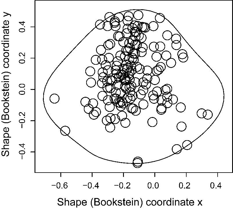
Figure 1. Spatial point pattern derived from pooled drilling data on Plio-Pleistocene specimens of the bivalve Lirophora latilirata from the Atlantic coastal plain.
Creating Spatial Point Patterns of Drilling Locations
A key feature of the SPPAT approach is the creation of a point pattern of drilling predation traces derived via geometric morphometrics. To accomplish this task, all landmark data on drillhole locations for L. latilirata and I. subrugosa were separately pooled and superimposed on a standardized skeleton to create a point pattern, that is, a representation of a given area containing a set of locations (hereafter referred to as “L. latilirata samples” and “beach-collected samples,” respectively; Figs. 2, 3). The pooled point pattern of predation traces on L. latilirata (Fig. 1) was further grouped into subpatterns (sensu Baddeley et al. Reference Baddeley, Rubak and Turner2016) according to geologic age, which are also referred here as point patterns and used to illustrate temporal changes in site-selectivity patterns, including variations in alternative shell-drilling behaviors.

Figure 2. Point patterns, kernel density, and hotspot maps of drillholes on fossil samples of Lirophora latilirata from the Atlantic coastal plain grouped by time interval. A, Late Pliocene. B, Early Pleistocene. C, Middle Pleistocene. Kernel density estimated using drilling frequency (DF) as a weighting variable. Units of density maps are number of drillholes per area measured in square Bookstein shape units. Hotspots were detected from the kernel density map using as a threshold the highest 10% estimated values.

Figure 3. Point patterns, kernel density, and hotspot maps derived from drilling data on beach-collected samples of Iliochione subrugosa (Playa Veracruz and Playa El Palmar, eastern Pacific coast of Panama) and feeding trials of Notocochlis unifasciata preying upon I. subrugosa. A, Beach samples. B, Feeding trial samples. Units of density maps are number of drillholes per area measured in square Bookstein shape units. Hotspots were detected from the kernel density map using as a threshold the highest 10% estimated values.
Kernel Density Estimation (KDE) and Hotspot Mapping
KDE was used to visualize the spatial distribution of predation traces on the prey skeleton for the modern beach-collected and laboratory feeding trial samples of I. subrugosa. This technique fits a curved surface over each drilling location such that the surface is highest above the drillhole and zero at a specified distance (bandwidth, h) from the drillhole. Following Silverman (Reference Silverman1986: p. 76, Eq. 4.5), the kernel density was mathematically expressed as:
 $$f\lpar x \rpar = \displaystyle{1 \over {nh}}.\sum\nolimits_{i = 1}^n {} \displaystyle{{K\lpar {x-X_i} \rpar } \over h}$$
where ƒ(x) is the density value at drillhole location x, n is the number of drillholes, h is the bandwidth, x − X i is the distance to each drillhole location i, and K is the quadratic kernel function, which is defined as
 $$K\lpar x \rpar = \displaystyle{3 \over 4}\lpar {1-x^2} \rpar \comma \;\;\vert x \vert \le 1$$
 $$K\lpar x \rpar = 0\comma \;x \gt 1.$$
Because fossil samples of L. latilirata, unlike our modern beach-collected and laboratory feeding trial samples of I. subrugosa, came from several field surveys, and museum lots examined varied greatly in size, KDE estimates may be biased. Therefore, we implemented a correction for sampling effort using drilling frequency. Drilling frequency (DF) was calculated for each fossil lot l following Kowalewski (Reference Kowalewski, Kowalewski and Kelley2002: p. 19, Eq. 5):
 $${\rm DF}\lpar l \rpar = \displaystyle{{\;n_l} \over {0.5m_l}}\comma \;\;m_l \ge 1$$
where nl is the number of valves drilled in the museum lot l, and ml is the total number of valves in the same lot l. DF was used to reweight the KDE estimated at each drillhole location x and thus to control for the role of different museum lots in the resulting site-selectivity patterns. Drillholes from museum lots with higher DF were assigned greater weight and receive higher KDE estimates. This standard procedure for reweighting the contributions from the individual predatory traces can be used for density estimation when observations are sampled nonuniformly (Fieberg Reference Fieberg2007). In our study, for instance, museum lots with large numbers of specimens and an unusually high occurrence of edge-drilling may bias density patterns when pooling drilling data.
The optimum bandwidth h opt required for KDE was based on the number of predatory traces and the average distance from each trace to the mean center (e.g., standard distance) (Fotheringham et al. Reference Fotheringham, Brunsdon and Charlton2000). Descriptive statistics and parameters employed to calculate the optimum bandwidth h opt used for the KDE are presented in Table 2. Because drillhole configurations are scaled and aligned on the baseline of coordinates (−0.5, 0) and (0.5, 0) derived from Bookstein registration, measurement units (e.g., millimeters) cannot be provided for the density maps. KDE was performed using the function density.ppp (grid spacing eps = 0.01 map units; h = h opt; weights = DF) in the R package Spatstat v. 1.23-4 (Baddeley and Turner Reference Baddeley and Turner2005). Based on the estimated density, preferences in drilling location by predators can be reliably characterized as hotspots of drilling traces on the prey skeleton. Operationally, hotspot areas were detected from the kernel estimate map using the highest 10% of kernel estimated values as a threshold (Nelson and Boots Reference Nelson and Boots2008).
Table 2. Descriptive statistics used to calculate the optimum bandwidth (h opt).

Distance-based Statistical Analyses
The spatial distribution of predation traces on a given prey skeleton may be classified as random (CSR), aggregated (individual traces are placed together delineating groups or clusters), or segregated (individual traces are placed farther apart than they would be in CSR) or some combination of these patterns at different distances on the prey skeleton. Here we describe the K- and L-functions, which are used for hypothesis testing, and applied the maximum clustering distance measurement to indicate the distance on the prey skeleton at which traces were clustered.
We used Ripley's K-function (Ripley Reference Ripley1976, Reference Ripley1977) to quantify the spatial point patterns of predation traces assembled here. This summary statistic is widely used to quantify deviations from CSR in a statistically consistent framework (Fotheringham et al. Reference Fotheringham, Brunsdon and Charlton2000; Baddeley et al. Reference Baddeley, Rubak and Turner2016). Following Ripley (Reference Ripley1988), the estimate of K(r) employed in this study was mathematically expressed as:
 $$K\lpar r \rpar = \displaystyle{a \over {n\lpar {n-1} \rpar }}\;\sum\nolimits_i {} \sum\nolimits_j {} I\lpar {d_{ij} \le r} \rpar e_{ij}$$
where a is the area of the standardized prey skeleton, n is the number of drillholes, and the sum is taken over all ordered pairs of drillholes i and j in the point pattern. dij is the distance between the two drillholes and I (dij ≤ r) is the indicator that equals 1 if the distance is less than or equal to r. The term eij is a standard correction factor to minimize potential bias from edge effects in estimating the K-function (Baddeley et al. Reference Baddeley, Rubak and Turner2016). The expected value of K(r) for a random Poisson distribution (K pois) is πr 2 and deviations from this expectation indicate either an aggregated or segregated distribution. This function provides the average number of neighboring drillholes that lie within a distance r of a drillhole divided by the density of drillholes per unit area or intensity. Because it is adjusted for intensity, the K-function makes it possible to compare the degree of regularity between point patterns of drillhole locations with different average densities (Baddeley et al. Reference Baddeley, Rubak and Turner2016), including both temporal and spatial comparisons. To facilitate the visual assessment of the graphic output, we used Besag's (Reference Besag1977) L-function, which transforms the K-function K pois(r) = πr2 to the straight-line L pois (r) = r:
 $$L\lpar r \rpar = \sqrt {\displaystyle{{k\lpar r \rpar } \over \pi }} .$$
The square-root transformation stabilizes the variance of the empirical L(r), making it easier to assess deviations from CSR and thus to evaluate the following scenarios: (1) null hypothesis [CSR]: L(r) = r; (2) alternative hypothesis 1 [aggregated]: L(r) > r; and (3) alternative hypothesis 2 [segregated]: L(r) < r. The nonparametric test for CSR in drillhole locations was constructed by simulating 999 random spatial patterns of size n from a homogeneous spatial Poisson process and taking the 50th largest among the simulated values (L theo) to achieve a desired significance level α = 50/(999 + 1). The empirical (L obs) and theoretical (L theo) L-functions were estimated for a range of r values measured in Bookstein shape coordinates using the Lest function, and critical values were computed using the envelope function. The point of maximum difference between the observed and expected L values (L obs − L theo), termed maximum clustering distance (MCD), was used to indicate the distance at which predation traces were aggregated (Mullins et al. Reference Mullins, Van Ert, Hadfield, Nikolich, Hugh-Jones and Blackburn2015). Because the K-function is cumulative and the graphic tool used for statistical inference may be difficult to interpret (Baddeley et al. Reference Baddeley, Rubak and Turner2016), we contrasted our results from the L-function against the pair correlation function (PCF). The PCF describes how the (normalized) density of predation traces changes as a function of distance, with the value PCF = 1 indicating CSR, PCF > 1 aggregation, and PCF < 1 segregation (Illian et al. Reference Illian, Penttinen, Stoyan and Stoyan2008). We contrasted our results against the nearest neighbor index (NNI) (Clark and Evans Reference Clark and Evans1954), a procedure that was previously used by Casey et al. (Reference Casey, Farrell, Dietl and Veilleux2015) to quantify deviations from CSR in the location of drilling predation traces. NNI is defined as the ratio of the mean nearest neighbor distance observed divided by the average distance between neighbors under CSR, with NNI < 1 indicating aggregation, and NNI > 1 segregation of traces. We also used a general approach that converts the results calculated at different distances along the prey skeleton into a single summary statistic u, the goodness-of-fit test (GoF) described by Loosmore and Ford (Reference Loosmore and Ford2006). The functions used for spatial statistical analyses are available in the R package Spatstat v. 1.23-4 (Baddeley et al. Reference Baddeley, Rubak and Turner2016).
Results
Description and Visualization of Spatial Patterns
Overall, the spatial point pattern of predation traces for L. latilirata samples showed that drillholes were spread around the shell wall, ranging from the anterior margin to the umbonal area, with some traces located directly on the shell margin near the ventral anterior and posterior regions (Fig. 1). When point patterns for fossil L. latilirata were grouped by geologic age and examined through time, areas of higher concentration of predation traces derived via kernel density were irregularly distributed on the prey skeleton (Fig. 2A–C). Hotspot maps indicate a subtle migration of a single hotspot of predation traces on the prey skeleton of L. latilirata through time, from the dorsal wall region in the late Pliocene (Fig. 2A) toward the central region of the wall area in the early Pleistocene (Fig. 2B) and the anterior region in the middle Pleistocene (Fig. 2C). Only a few cases of edge drilling, a mode of predation in which a predator drills a hole at a point on the commissure between the closed valves (Taylor Reference Taylor and Morton1980; Vermeij Reference Vermeij1980; Ansell and Morton Reference Ansell, Morton, Morton and Dudgeon1985; Mondal et al. Reference Mondal, Hutchings and Herbert2014; Rojas et al. Reference Rojas, Hendy and Dietl2015), were observed in the fossil L. latilirata samples, and thus no hotspots of predation traces were evident (Fig. 2).
In the point pattern of predation traces derived from beach-collected samples of I. subrugosa, two areas of higher concentration of drilling traces were found, one located at the umbo and the other a point placed at the ventral commissure, reflecting the occurrence of wall- and edge-drilling behavior of the unknown naticid predator(s). However, only a single hotspot was delimited by the analysis, corresponding to predation traces placed near the umbo, that is, wall drilling (Fig. 3A). In the point pattern of predation traces derived from feeding trials of N. unifasciata preying on I. subrugosa, we found a single area of higher concentration of drillholes as well as a single hotspot placed at the umbo (Fig. 3B) but slightly closer to the shell edge than in the beach-collected samples. In both beach-collected samples and feeding trial samples, the areas of higher concentration of drillholes covered a relatively small area of the prey skeleton when compared with those from fossil L. latilirata prey (Fig. 2).
Distance-based Statistics and Hypothesis Testing
The graphical output of the L-function indicated a significant aggregated pattern of predation traces across a range of distances on the skeleton of L. latilirata in both late Pliocene and early Pleistocene point patterns (Fig. 4A,B) (GoF: u = 0.001; p << 0.01). The average number of predation traces within a distance r shorter than 0.5 Bookstein shape units of another location (derived from Bookstein registration) was statistically greater than that expected for a complete random distribution. In addition, there was a reduction in the point of MCD from 0.25 to 0.19 Bookstein shape units for the late Pliocene to the early Pleistocene, respectively. The empirical PCF and L-function calculated for the middle Pleistocene point pattern remained entirely on the simulated envelopes, and thus there was insufficient evidence against the null hypothesis of CSR at any distance on the prey skeleton, a result supported by the GoF test (u = 0.001, p = 0.03).
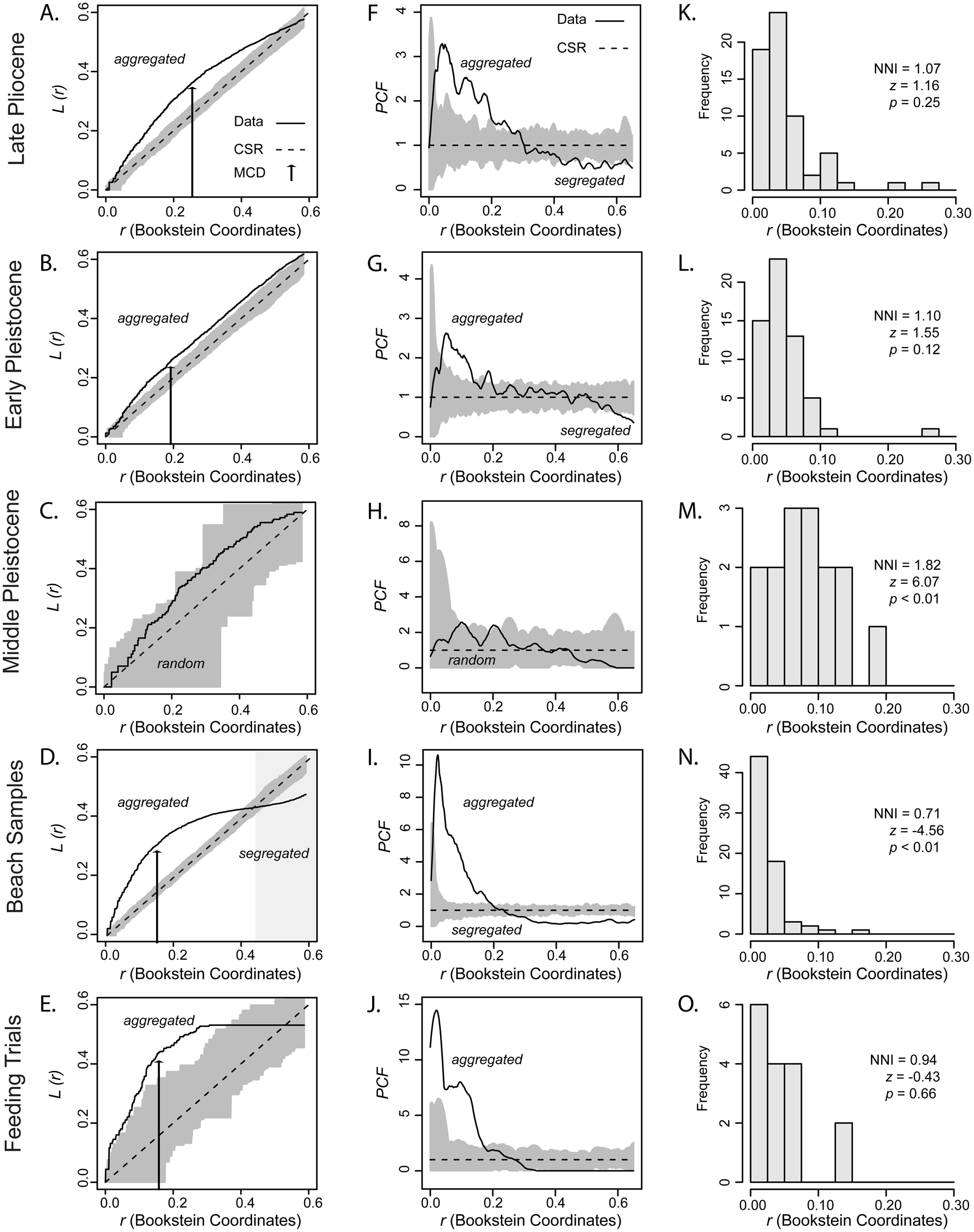
Figure 4. Graphical output from the distance-based statistics estimated on the fossil samples, modern beach-collected samples, and laboratory feeding trials. A–E, L-function. Black arrow indicates the point of maximum clustering distance (MCD). F–J, Pair correlation function (PCF). K–O, Histograms of nearest neighbor distances and estimated nearest neighbor index (NNI) for the actual data. Legend: Empirical (“Data”) and expected (complete spatial randomness, “CSR”) functions. The dark gray area is the simulation envelope for 999 Monte Carlo simulations of CSR. z, nearest neighbor z-score; a negative z-value indicates aggregation; a positive z-value indicates segregation.
The graphical output of the L-function calculated for the point pattern derived from the beach-collected samples of I. subrugosa indicates the occurrence of two segregated clusters, that is, a mixed pattern that includes aggregation and segregation at different distances on the prey skeleton (Fig. 4D) (GoF test for CSR: u = 0.005; p = 0.01). Predation traces located at short distances from other traces in the prey skeleton, either pairs of traces located on the umbo or the ventral margin, define the aggregated pattern. Pairs of predation traces located at large distances from each other, specifically those pairs that include one trace located on the umbo and another on the ventral margin, were located farther apart than expected under CSR, supporting a segregated pattern. In this case, the distance between traces approximates the length of the dorsoventral axis (Fig. 4D). In contrast, only an aggregated pattern of traces was observed for feeding trial data of N. unifasciata preying on I. subrugosa (GoF: u = 0.012; p << 0.01); thus, the segregated pattern observed in the beach-collected samples of the same prey species was not supported (Fig. 4E). Remarkably, the MCD in the point patterns derived from the beach-collected samples (0.15) and feeding trial samples (0.17) was similar.
Results from the L-function and PCF for the assembled point patterns are related but appear to capture different aspects of the distribution of predation traces over a range of distances on the prey skeleton (Fig. 4A–J). The L-function was more conservative, indicating a significant segregated pattern of traces at large distances (>0.45 Bookstein shape distance) exclusively in the beach-collected samples (Fig. 4D), whereas the PCF showed additional minor excursions below the confidence envelope between 0.5 and 0.6 Bookstein shape distances, suggesting a weak aggregated pattern in the late Pliocene (Fig. 4F), early Pleistocene (Fig. 4G), and feeding trial (Fig. 4J) point patterns. The PCF also exhibited multiple peaks indicating aggregation of traces across the prey skeleton that could be attributed to multiple predators preying upon the examined prey (Fig. 4F–G,I–J), but a satisfactory interpretation of such peaks is not straightforward. In contrast, the L-function clearly identified two segregated clusters of traces on the beach-collected samples separated by more than 0.5 Bookstein shape distance, roughly corresponding to the distance separating the two areas with high density of traces in the KDE map (Fig. 2A) and corresponding to edge- and wall-drilling modes of predation (Rojas et al. Reference Rojas, Hendy and Dietl2015). The PCF indicated that such a pattern emerges at shorter distances (Bookstein shape distances > 0.3), which is consistent with segregated clusters located relatively closer to each other, either on the shell wall or shell edge, an observation that is not supported by KDE and hotspot maps. The NNI (Fig. 4F–J), previously used by Casey et al. (Reference Casey, Farrell, Dietl and Veilleux2015) to study site selectivity in drilling predation, provided little information on the spatial distribution of predation traces across different distances on the prey skeleton. The NNI did not capture the segregated pattern of traces in beach-collected samples (Fig. 4N) and even contradicted results that are consistent across the different distance-based functions implemented in our study, for example, the NNI indicated significant segregation of traces (NNI > 1; p < 0.01) for the middle Pleistocene point pattern, which was found to be random by both L-function and PCF.
Discussion
Spatial Patterns in the Distribution of Predation Traces on the Prey Skeleton
Kernel density maps show significant variation in the concentration of predation traces on the skeleton of fossil L. latilirata. The estimated L-function indicates that naticid predation traces on late Pliocene and early Pleistocene samples, which likely included the abundant Naticarius canrena (Linnaeus, Reference Linnaeus1758), Naticarius plicatella (Conrad, Reference Conrad1863), and Neverita duplicata (Say, Reference Say1822) found in the same surveyed bulk samples (Supplementary Table S2), are significantly aggregated. Hotspots of predation traces in the late Pliocene and early Pleistocene spatial point patterns are unique, restricted to wall-drilling cases, and range in location from the middle region of the shell to the umbo. Predation traces in the middle Pleistocene point pattern were randomly placed (Figs. 4C,H). However, because naticid drilling predation tends to be a stereotyped behavior (Kabat Reference Kabat1990; Kingsley-Smith et al. Reference Kingsley-Smith, Richardson and Seed2003; Rojas et al. Reference Rojas, Hendy and Dietl2015), this pattern is likely due to small sample size. The observed reduction in the MCD from late Pliocene to early Pleistocene point patterns for L. latilirata may represent either temporal increase in site selectivity or changes in predator assemblages. The diversity of naticid species recorded in samples from the surveyed geologic units decreases from 19 to 8 between the late Pliocene and early Pleistocene samples, with at least five species in common (Supplementary Table S2). Although we cannot distinguish the individual contribution of each predator to the observed pattern in concentration of predation traces, we observed a temporal shift in hotspot locations migrating toward the ventral area of the shell. Demonstrating temporal shifts in site-selectivity preferences of drilling predators requires replicated samples through several stratigraphic sections, a task that is beyond the scope of this paper. Instead, this case study illustrates how MCD may provide information on temporal changes in site-selectivity preferences. Our results also indicate that L. latilirata was not subject to significant edge-drilling attacks, pointing to the rarity of such predatory behavior in the examined fossil samples.
Although only a single hotspot characterizes the spatial distribution of predation traces from unknown naticid predators preying on I. subrugosa in the beach-collected samples, distance-based statistical analysis indicates cluster segregation, that is, predation traces are significantly aggregated at small scales or short distances and yet simultaneously significantly distributed in a segregated pattern at large distances on the prey skeleton (Fig. 4D). The segregated pattern results from the high concentration of predation traces located at short distances, either on the umbo or at the ventral edge, which gives an MCD of 0.25 Bookstein shape units. In contrast, the segregated pattern results from the concentration of predation traces at a larger distance on the prey skeleton, which approximates the distance (0.45 Bookstein shape units) separating the umbo and the ventral edge (i.e., dorsoventral axis) (Fig. 4D). The distance on the prey skeleton at which the PCF indicates clustered aggregation (Fig. 4I) is significantly shorter than the dorsoventral axis, pointing to the advantage of the L-function over the PCF in characterizing distribution of predation traces. This case study also highlights the need for combining density estimation, hotspot mapping, and distance-based functions to best characterize the distribution of predation traces on prey.
A previous qualitative analysis of site-selectivity patterns between the studied beach-collected and laboratory feeding trial samples used in this study suggested the occurrence of similar drilling patterns (Rojas et al. Reference Rojas, Hendy and Dietl2015). Despite similarities (e.g., occurrence of edge drilling, similar MCD), distance-based statistical analysis indicated that the number of predation traces located on the ventral edge of I. subrugosa in the feeding trials is not enough to form a significant segregated pattern as was the case for the beach-collected samples. This evidence may point to biased site-selectivity patterns either due to artifacts under laboratory conditions (e.g., lack of competition may reduce incidence of edge-drilling behavior; Dietl Reference Dietl2004) or the influence of sample size (e.g., small sample sizes may not resolve minor peaks in density of predation traces), which should be further explored. This case study also illustrates the value of the SPPAT framework over qualitative assessments of site selectivity in evaluating alternative modes of drilling predation (i.e., edge and wall drilling).
Site-Selectivity Assessment Using SPPAT
Current methods to characterize site-selectivity patterns of drilling predators exclude some spatial information inherent to drillhole location, employing an oversimplified description of the trace position, for example, distance of the drillhole to a selected feature in the skeleton (Kowalewski Reference Kowalewski, Kowalewski and Kelley2002). The SPPAT approach implemented here exploits the spatially explicit nature of the drilling traces to accurately map predation traces on both modern and fossilized shelled invertebrate prey to provide visual and quantitative information on subtle differences in site-selectivity patterns that are not apparent to the naked eye (see Illian et al. Reference Illian, Penttinen, Stoyan and Stoyan2008; Mitchell and Butterfield Reference Mitchell and Butterfield2018; Mitchell et al. Reference Mitchell, Kenchington, Harris and Wilby2018), including recognition of the slight migration of hotspots along particular regions of the prey skeleton that otherwise would be described ambiguously (e.g., shell wall and shell edge) or that depend critically on the arbitrary grid system used by sector-based approaches (Kowalewski Reference Kowalewski1990, Reference Kowalewski, Kowalewski and Kelley2002). Limitations of sector-based methods for spatial analysis have been recognized previously in other research fields, such as archaeology (Hodder and Okell Reference Hodder, Okell and Hodder1978; Johnson Reference Johnson and Hietala1984) and ecology (Culley et al. Reference Culley, Campbell and Canfield1933; Elliott Reference Elliott1971). Because distance-based statistics for hypothesis testing are included (Ripley's K-function, L-function, and PCF), the SPPAT approach quantifies complex patterns that emerge at different distances on the prey skeleton (e.g., mixing of aggregated and segregated patterns) that cannot be captured using either sector-based methods (Hodder and Okell Reference Hodder, Okell and Hodder1978) or nearest neighbor statistics (Li and Zhang Reference Li and Zhang2007). The nearest neighbor approach implemented by Casey et al. (Reference Casey, Farrell, Dietl and Veilleux2015) is useful for testing the CSR hypothesis and identifying local associations but not for quantifying scale-dependent patterns. Our results support the notion that the NNI is unreliable in the recognition of complex spatial patterns in the distribution of predation traces on shelled invertebrate prey. Li and Zhang (Reference Li and Zhang2007) and Mitchell and Butterfield (Reference Mitchell and Butterfield2018) discussed other examples for which nearest neighbor statistics were also found to be unreliable in the study of spatial patterns.
Although we illustrated the SPPAT approach through case studies of naticid gastropod predation on bivalve prey, it could be extended to examine the composite pattern of predatory traces produced by co-occurring predators (e.g., naticid and muricid gastropods) relative to each group. In addition, drillhole diameter or any other attribute (predator taxonomy, length, etc.) of the predation traces could be used to create a marked point pattern and thus to explore its effect on the spatial patterns.
Conclusions
Site-selectivity analysis of shell-drilling predators is a spatially explicit question. Taking advantage of the spatial information inherent to drillhole location, the SPPAT approach developed here captures diverse aspects in the spatial distribution of predation traces on modern and fossilized prey remains and introduces a novel set of graphic (i.e., kernel density and hotspot maps) and quantitative tools (i.e., K-function, L-function, MCD), largely used in research fields other than paleobiology, for evaluating changes in site-selectivity patterns across taxa, space, and time. Despite limitations affecting data used here—both stratigraphic (i.e., long and unequal time intervals) and geographic (i.e., sampling localities relatively far apart from each other and potential variation in sampled environments)—we showed how SPPAT can be used to visualize areas of high concentration of predation traces on the prey skeleton and to quantify aggregated and segregated patterns occurring at different spatial scales (or distances on the prey skeleton). The visual information on density of predation traces and hotspots, as well the identification of mixed spatial patterns, could not have been obtained using current approaches that lack spatial information and that are dependent on the scale of analysis. We also showed that the point of MCD is an informative measure to examine large-scale temporal and small (intravalve) spatial-scale variation in site-selectivity patterns. Future studies could investigate variation in hotspot locations and MCD in terms of large-scale geographic variation (e.g., latitudinal trends), co-occurring predators (e.g., naticids and muricids), and prey variables, such as taxonomy, thickness, size, mode of life, and ornamentation that are important to this predator–prey interaction. Our study provides a general conceptual framework to orient future research on site-selectivity patterns in drilling predation. However, the SPPAT approach may be generalized to a wide spectrum of ecologic and taphonomic data preserved on skeletal remains of Phanerozoic marine invertebrates, including encrustation, bioerosion traces, and repair scars (Kowalewski Reference Kowalewski, Kowalewski and Kelley2002) that are spatially explicit and can be mapped.
Acknowledgments
We thank S. Roberts (Division of Invertebrate Paleontology, FLMNH) for assistance in the museum survey. We thank two anonymous reviewers and editor M. Patzkowsky for helpful comments and constructive criticism that greatly improved this article. A.R. is grateful to E. Sandoval for her continuous support. A.R. was supported by the Olle Engkvist Byggmästare Foundation. Financial support to R.W.P. for fieldwork was kindly provided by Mrs. Barbara and son James Toomey and the McGinty Endowment (FLMNH). This is University of Florida Contribution to Paleobiology 853.


 Open access