


1. Introduction
The equilibrium distribution (also named stationary renewal distribution) arises as the limiting distribution of the forward recurrence time in a renewal process, see Cox [Reference Cox7]. It represents a relevant concept in reliability theory and survival analysis (see, for instance, Section 1.A.5 in Shaked and Shanthikumar [Reference Shaked and Shanthikumar31]), actuarial and risk theory (see, for example, Willmot [Reference Willmot32]). Let X be a non-negative random variable, with survival function (SF)  $\overline{F}(t)=\mathsf{P}(X \gt t)$, for
  $t\ge 0$, and mean
  $\mu=\mathsf{E}[X]=\int_{0}^{+\infty}\overline{F}(t){\rm d}t$ such that
  $0 \lt \mu \lt +\infty$. The equilibrium random variable of X, denoted as Xe, has (decreasing) probability density function (PDF)
 \begin{equation}
f^e(t)=\frac{\overline{F}(t)}{\mu},\qquad t\ge 0.
\end{equation}
\begin{equation}
f^e(t)=\frac{\overline{F}(t)}{\mu},\qquad t\ge 0.
\end{equation} Then, the SF of Xe is given by  $\overline{F}^e(t)=\pi(t)/\mu$, for
  $t\ge 0$, where
 \begin{equation*}
\pi(t)=\mathsf{E}[(X-t)_+]=\int_{t}^{+\infty}\overline{F}(x){\rm d}x,\qquad t\ge 0,
\end{equation*}
\begin{equation*}
\pi(t)=\mathsf{E}[(X-t)_+]=\int_{t}^{+\infty}\overline{F}(x){\rm d}x,\qquad t\ge 0,
\end{equation*}denotes the stop-loss transform of X, see Section 1.7 in Denuit et al. [Reference Denuit, Dhaene, Goovaerts and Kaas9].
In the present work, we define a generalized version of the equilibrium PDF given in Eq. (1.1), for the case in which the baseline random variable X has a general support. We extend the probabilistic generalization of Taylor’s theorem (cf. Massey and Whitt [Reference Massey and Whitt20]) to this case. Conditions for which the mean, median, and mode of such PDF coincide and are equal to zero are illustrated too. Moreover, under suitable assumptions, we prove that many stochastic comparisons between baseline distributions are maintained by the corresponding generalized equilibrium ones. The sign of the median of the baseline distribution leads to the preservation of various aging properties.
We go further by extending to general supports the equilibrium PDF of two ordered random variables studied in Di Crescenzo [Reference Di Crescenzo11] and Psarrakos [Reference Psarrakos27] for non-negative random variables, and in Psarrakos [Reference Psarrakos28] for Poisson and Normal distributions. Along this line, a probabilistic analog of the mean value theorem is proved by using the new probabilistic generalization of Taylor’s theorem. Further results and stochastic comparisons are provided as well.
We often consider distortion-based models, that allow us to avoid conditions on the involved distributions. In particular, some illustrative examples deal with families of distortion functions related to the well-known proportional hazard rate (PHR) model (see Cox [Reference Cox8] and Kumar and Klefsjö [Reference Kumar and Klefsjö17]) and proportional reversed hazard rate (PRHR) model (see Di Crescenzo [Reference Di Crescenzo12] and Gupta and Gupta [Reference Gupta and Gupta14]).
The concept of unimodal PDF plays a relevant role throughout the paper. Under a (weak) suitable assumption on the baseline distribution, we emphasize that the proposed generalized equilibrium PDF is unimodal, with mode zero. In addition, we study conditions for the unimodality of the extended equilibrium PDF of two ordered random variables. Unimodality issues are relevant in actuarial science, since the distribution of insurance loss data is often unimodal, see Punzo et al. [Reference Punzo, Bagnato and Maruotti29] and references therein. Moreover, stochastic comparisons play a significant role in economics and insurance, see Belzunce et al. [Reference Belzunce, Pinar, Ruiz and Sordo4], Müller [Reference Müller18], and Sánchez-Sánchez et al. [Reference Sánchez-Sánchez, Sordo, Suárez-Llorens and Gómez-Déniz30]. Hence, we apply such equilibrium PDFs in risk theory by studying the connection with the Lorenz curve, stochastic orderings, and unimodality problems between risks and their truncated versions at the respective Value-at-Risk (VaR).
The paper is organized as follows. In Section 2, we recall some basic notions. Section 3 is devoted to the definition of the new equilibrium random variable, by describing related properties and results. Many stochastic orders and aging classes are preserved through generalized equilibrium transformations, as shown in Section 4. Various results concerning the equilibrium PDF of two ordered random variables with support in  $\mathbb{R}$ are provided in Section 5. Finally, in Section 6, we apply the equilibrium PDFs described above in actuarial and insurance contexts. Some final remarks are given in Section 7.
2. Background
In this section, we fix the notation and we recall some useful notions, such as unimodality, stochastic orders, aging classes, and distortion functions. Throughout the paper, the terms increasing and decreasing are used, respectively, as “non-decreasing” and “non-increasing,” while “iff” denotes “if and only if.”
Given a probability space  $(\Omega,\mathcal{F},\mathsf{P})$, let
  $X\colon\Omega\rightarrow\mathbb{R}$ be a random variable, with SF
  $\overline{F}$ and cumulative distribution function (CDF)
  $F=1-\overline{F}$. The function
  $F^{-1}(u)=\sup\{t\colon F(t)\leq u\}$, for
  $u\in[0,1]$, represents the right-continuous version of the inverse of F, namely quantile function. Moreover, we denote by
  $\overline{F}^{-1}(u)=F^{-1}(1-u)$, for all
  $u\in[0,1]$.
It is well-known that  $X=X^{+}-X^{-}$, where
 \begin{equation}
X^{+}=\max(0,X)\quad\text{and}\quad X^{-}=\max(-X,0),
\end{equation}
\begin{equation}
X^{+}=\max(0,X)\quad\text{and}\quad X^{-}=\max(-X,0),
\end{equation}are non-negative random variables that represent the positive and negative parts of X, respectively. Therefore, by denoting with
 \begin{equation}\mu^{+}=\mathsf{E}[X^{+}]=\int_{0}^{+\infty}\overline{F}(t){\rm d}t\quad\text{and}\quad\mu^{-}=\mathsf{E}[X^{-}]=\int_{-\infty}^{0}F(t){\rm d}t,\end{equation}
the mean of X can be computed as
 \begin{equation}
\mu=\mathsf{E}[X]=\mu^{+}-\mu^{-}
\end{equation}
\begin{equation}
\mu=\mathsf{E}[X]=\mu^{+}-\mu^{-}
\end{equation} and µ exists (is finite) iff  $\mu^{+},\mu^{-}\in\mathbb{R}$. In addition, since
  $|X|=X^{+}+X^{-}$ one has
 \begin{equation}
\tilde{\mu}=\mathsf{E}[|X|]=\mu^{+}+\mu^{-}.
\end{equation}
\begin{equation}
\tilde{\mu}=\mathsf{E}[|X|]=\mu^{+}+\mu^{-}.
\end{equation} The variance of X is  $\mathsf{V}[X]=\mathsf{E}\left[(X-\mu)^2\right]$. Moreover, every
  $m\in\mathbb{R}$ such that
 \begin{equation*}
\frac12\le F(m)\le\frac12+\mathsf{P}(X=m)
\end{equation*}
\begin{equation*}
\frac12\le F(m)\le\frac12+\mathsf{P}(X=m)
\end{equation*} is named median of X and therefore, if  $\mathsf{P}(X=m)=0$, then
  $F(m)=1/2$.
It is well-known that the mode of a given dataset is the value that appears most often. In particular, if X has a discrete distribution, then  $\nu={\rm argmax}_{x}\mathsf{P}(X=x)$ denotes a mode of X. In the absolutely continuous case, a mode of X is any value ν in which its PDF
  $f=F'$ has a maximum. We consider the following formal definition of unimodality.
Definition 2.1. Let X be a random variable with absolutely continuous CDF F. We say that X is unimodal about a unique mode ν if F is strictly convex on  $(-\infty,\nu)$ and strictly concave on
  $(\nu,+\infty)$.
In other words, due to Definition 2.1, X is unimodal iff it has a PDF  $f$ with a single peak in
  $f(\nu)$, with ν mode of X. In this sense, the Normal (or Gaussian) and the Cauchy distributions are both unimodal, while the continuous uniform distribution is not unimodal. For more details about unimodality we refer the reader to Dharmadhikari and Joag-Dev [Reference Dharmadhikari and Joag-Dev10].
Hereafter, we recall a suitable version of the probabilistic generalization of Taylor’s theorem given in Massey and Whitt [Reference Massey and Whitt20] for non-negative random variables that involves the equilibrium PDF in Eq. (1.1).
Theorem 2.1. Let X be a non-negative random variable with CDF F and  $0 \lt \mathsf{E}[X] \lt +\infty$. Let
  $h:[0,+\infty)\rightarrow\mathbb{R}$ be a measurable and differentiable function for
  $t\in(0,+\infty)$ such that h(0) is finite. Let its derivative h′ be measurable and Riemann-integrable. If
  $\mathsf{E}[h'(X^e)]$ is finite, then
  $\mathsf{E}[h(X)]$ is finite and
  $\mathsf{E}[h(X)]=h(0)+\mathsf{E}[X]\mathsf{E}[h'(X^e)]$.
Now we define some well-known aging functions that are useful in reliability theory and survival analysis, where a non-negative random variable describes the lifetime of a single component or a system built with some components. More in general, for a random variable X having support in  $\mathbb{R}$, let
  $X_t=\left[X-t|X \gt t\right]$ denote the residual lifetime of X at age
  $t\in\mathbb{R}$. The mean residual lifetime (MRL) of X is computed as
 \begin{equation*}
\zeta(t){\,:=\,}\mathsf{E}\left[X_t\right]=\frac1{\overline{F}(t)}\int_{t}^{+\infty}\overline{F}(x){\rm d}x,\qquad t\in\mathbb{R}:\, \overline{F}(t) \gt 0.
\end{equation*}
\begin{equation*}
\zeta(t){\,:=\,}\mathsf{E}\left[X_t\right]=\frac1{\overline{F}(t)}\int_{t}^{+\infty}\overline{F}(x){\rm d}x,\qquad t\in\mathbb{R}:\, \overline{F}(t) \gt 0.
\end{equation*} Moreover, if  $X_{(t)}=\left[t-X|X\le t\right]$ denotes the inactivity time of X, then the mean inactivity time (MIT) of X is expressed as
 \begin{equation*}
\tilde{\zeta}(t){\,:=\,}\mathsf{E}\left[X_{(t)}\right]=\frac1{F(t)}\int_{-\infty}^{t}F(x){\rm d}x,\qquad t\in\mathbb{R}:\, F(t) \gt 0.
\end{equation*}
\begin{equation*}
\tilde{\zeta}(t){\,:=\,}\mathsf{E}\left[X_{(t)}\right]=\frac1{F(t)}\int_{-\infty}^{t}F(x){\rm d}x,\qquad t\in\mathbb{R}:\, F(t) \gt 0.
\end{equation*} Note that, from Eqs. (2.2) and (2.3), one has  $\mu=\overline{F}(0)\zeta(0)-F(0)\tilde{\zeta}(0)$.
If X has an absolutely continuous distribution, then its hazard rate (HR) is defined as  $\lambda(t){\,:=\,} f(t)/\overline{F}(t)$, for all
  $t\in\mathbb{R}$ such that
  $\overline{F}(t) \gt 0$, while its reversed hazard rate (RHR) is defined as
  $\tau(t){\,:=\,} f(t)/F(t)$, for all
  $t\in\mathbb{R}$ such that
  $F(t) \gt 0$. Moreover, if X has differentiable PDF f, then the ratio
 \begin{equation*}
\eta(t){\,:=\,}-\frac{f'(t)}{f(t)},\qquad t\in\mathbb{R}:\, f(t) \gt 0,
\end{equation*}
\begin{equation*}
\eta(t){\,:=\,}-\frac{f'(t)}{f(t)},\qquad t\in\mathbb{R}:\, f(t) \gt 0,
\end{equation*}is the Glaser’s function of X, see Glaser [Reference Glaser13] and Navarro [Reference Navarro21].
We now are ready to recall some stochastic orders. Here  $a/0$ is taken to be equal to
  $+\infty$ whenever a > 0. Moreover, the subscript refers to the random variables.
Definition 2.2. We say that X is smaller than Y in the
• usual stochastic order, denoted by
 $X\le_{st}Y$, if
$\overline{F}_X(t)\le\overline{F}_Y(t)$ holds for all t. If there is equality in law, then we write
$X=_{st}Y$;
$X\le_{st}Y$, if
$\overline{F}_X(t)\le\overline{F}_Y(t)$ holds for all t. If there is equality in law, then we write
$X=_{st}Y$;• increasing convex order, denoted by
$X\le_{icx}Y$, if
$\int_{t}^{+\infty}\overline{F}_X(s){\rm d}s\le\int_{t}^{+\infty}\overline{F}_Y(s){\rm d}s$ holds for all t;• increasing concave order, denoted by
$X\le_{icv}Y$, if
$\int_{-\infty}^{t}F_X(s){\rm d}s\ge\int_{-\infty}^{t}F_Y(s){\rm d}s$ holds for all t;• convex order, denoted by
$X\le_{cx}Y$, if
$\int_{t}^{+\infty}\overline{F}_X(s){\rm d}s\le\int_{t}^{+\infty}\overline{F}_Y(s){\rm d}s$ and
$\int_{-\infty}^{t}F_X(s){\rm d}s\le\int_{-\infty}^{t}F_Y(s){\rm d}s$ hold for all t;• hazard rate order, denoted by
$X\le_{hr}Y$, if
$\overline{F}_X(t)/\overline{F}_Y(t)$ is decreasing in t;• reversed hazard rate order, denoted by
$X\le_{rhr}Y$, if
$F_X(t)/F_Y(t)$ is decreasing in t;• mean residual lifetime order, denoted by
$X\le_{mrl}Y$, if
$\zeta_X(t)\le\zeta_Y(t)$ holds for all t;• mean inactivity time order, denoted by
$X\le_{mit}Y$, if
$\tilde{\zeta}_X(t)\ge\tilde{\zeta}_Y(t)$ holds for all t;• likelihood ratio order, denoted by
$X\le_{lr}Y$, if
$f_X(t)/f_Y(t)$ is decreasing for t in the union of their supports, provided that X and Y have absolutely continuous distributions.


In the absolutely continuous case, one has  $X\le_{hr}Y$ iff
  $\lambda_X(t)\ge\lambda_Y(t)$ for all t, while
  $X\le_{rhr}Y$ iff
  $\tau_X(t)\le\tau_Y(t)$ for all t. Moreover, when fX and fY are both differentiable, one has
  $X\le_{lr}Y$ iff
  $\eta_X(t)\ge\eta_Y(t)$ for all t in the union of their supports. In Table 1, we include the relationships among the stochastic orders introduced in Definition 2.2. The proof of these relationships with a detailed description of stochastic orders and applications can be found in Belzunce et al. [Reference Belzunce, Martínez-Riquelme and Mulero3], Denuit et al. [Reference Denuit, Dhaene, Goovaerts and Kaas9], Kochar [Reference Kochar16], Müller and Stoyan [Reference Müller and Stoyan19], and Shaked and Shanthikumar [Reference Shaked and Shanthikumar31] (in particular, for the mean inactivity time order, see Ahmad et al. [Reference Ahmad, Kayid and Pellerey1] and references therein).
Relationships among the stochastic orders introduced in Definition 2.2, where µX and µY denote the mean of X and Y, respectively.

In the following, we define some useful aging classes.
Definition 2.3. A random variable X is
• increasing failure (or hazard) rate (IFR) if
$X_t\ge_{st}X_{s}$ whenever
$t\le s$ in
$\mathbb{R}$. If
$X_t\le_{st}X_{s}$ whenever
$t\le s$ in
$\mathbb{R}$, then X is decreasing failure rate (DFR);• decreasing reversed failure (or hazard) rate (DRFR) if
$X_{(t)}\le_{st}X_{(s)}$ whenever
$t\le s$ in
$\mathbb{R}$;• decreasing in mean residual lifetime (DMRL) if
$\zeta(t)$ is decreasing for
$t\in\mathbb{R}$;• increasing in mean inactivity time (IMIT) if
$\tilde{\zeta}(t)$ is increasing for
$t\in\mathbb{R}$;• increasing in likelihood ratio (ILR) if f is log-concave, provided that X has an absolutely continuous distribution.


In the absolutely continuous case one can also say that X is IFR (DFR) iff  $\overline{F}$ is log-concave (log-convex), i.e., its HR λ is increasing (decreasing), while X is DRFR iff F is log-concave, i.e., its RHR τ is decreasing. Moreover, if f is differentiable, then X is ILR iff its Glaser’s function η is increasing. The relationships among the aging classes introduced in Definition 2.3 are shown in Table 2. For more details about aging notions, we address the reader to Belzunce et al. [Reference Belzunce, Martínez-Riquelme and Mulero3], Kochar [Reference Kochar16], Section 4 in Navarro [Reference Navarro22], Navarro et al. [Reference Navarro, Ruiz and Del Aguila25] and Shaked and Shanthikumar [Reference Shaked and Shanthikumar31].
Relationships among the aging classes introduced in Definition 2.3.

We conclude this section by recalling the concept of distortion function, introduced by Yaari [Reference Yaari33] in the context of the theory of choice under risk. In particular, given F, a distorted CDF  $F_q=q(F)$ can be obtained making use of an increasing continuous function
  $q:[0,1]\rightarrow[0,1]$, such that
  $q(0)=0$ and
  $q(1)=1$, namely distortion function. Moreover, the function
  $\tilde{q}(u){\,:=\,}1-q(1-u)$, for
  $u\in[0,1]$, is called dual distortion function respect to q. Then
  $\overline{F}_q=\tilde{q}(\overline{F})$ is the distorted SF from
  $\overline{F}$ through
  $\tilde{q}$. Further details about distortion functions can be found in Section 2.4 in Navarro [Reference Navarro22].
3. Generalized equilibrium distribution
In this section, we introduce and study the generalized equilibrium distribution of a given random variable. In particular, we extend the definition of the equilibrium PDF given in Eq. (1.1) for non-negative random variables to the case in which the baseline random variable has a general support. Along this line, we provide a new probabilistic version of Taylor’s theorem and we discuss mean-median-mode relations. By recalling Eq. (2.2), the formal definition of generalized equilibrium random variable can be stated as follows.
Definition 3.1. Let X be a non-degenerate random variable, having CDF F, SF  $\overline{F}$, and finite mean. The generalized equilibrium random variable of X, denoted as Xe, has the following PDF
 \begin{equation}
\displaystyle
f^{e}(t)=
\begin{cases}
\displaystyle\frac{F(t)}{\tilde{\mu}},& t \lt 0, \\[3mm]
\displaystyle\frac{\overline{F}(t)}{\tilde{\mu}},& t\ge0, \\
\end{cases}
\end{equation}
\begin{equation}
\displaystyle
f^{e}(t)=
\begin{cases}
\displaystyle\frac{F(t)}{\tilde{\mu}},& t \lt 0, \\[3mm]
\displaystyle\frac{\overline{F}(t)}{\tilde{\mu}},& t\ge0, \\
\end{cases}
\end{equation} where  $\tilde{\mu}=\mu^{+}+\mu^{-} \gt 0$.
From Eq. (2.4), it is easy to see that the function  $f^e$ in Eq. (3.1) is a proper PDF, which is increasing for t < 0 and decreasing for
  $t\ge0$. Clearly, if X is non-negative, then Eq. (3.1) reduces to Eq. (1.1).
Given X, by recalling Eq. (2.1), the PDF of  $(X^+)^e$ arises as limiting distribution of the age of a renewal process having independent and identically distributed interarrival times according to
  $X^+$. Similar considerations follow for
  $X^-$. In this sense, the mixture representation provided in the following remark allows us to connect the generalized equilibrium PDF defined in Eq. (3.1) with Renewal Theory.
Remark 3.1. By recalling Eq. (2.1), let us denote with  $f_{-}^e$ the PDF of
  $-(X^-)^e$, and with
  $f_{+}^e$ the PDF of
  $(X^+)^e$. Therefore, from Eqs. (2.2) and (3.1) one has
 \begin{equation*}
f^{e}(t)=
\begin{cases}
\displaystyle\frac{\mu^{-}}{\tilde{\mu}}f_{-}^e(t),& t \lt 0, \\[3mm]
\displaystyle\frac{\mu^{+}}{\tilde{\mu}}f^{e}_{+}(t),& t\ge0, \\
\end{cases}
\end{equation*}
\begin{equation*}
f^{e}(t)=
\begin{cases}
\displaystyle\frac{\mu^{-}}{\tilde{\mu}}f_{-}^e(t),& t \lt 0, \\[3mm]
\displaystyle\frac{\mu^{+}}{\tilde{\mu}}f^{e}_{+}(t),& t\ge0, \\
\end{cases}
\end{equation*}or, equivalently,
 \begin{equation*}
f^{e}(t)=pf_{-}^e(t)+(1-p)f^{e}_{+}(t),\qquad t\in\mathbb{R},
\end{equation*}
\begin{equation*}
f^{e}(t)=pf_{-}^e(t)+(1-p)f^{e}_{+}(t),\qquad t\in\mathbb{R},
\end{equation*} where  $p=\mu^{-}/\tilde{\mu}\in[0,1]$. Hence, Xe is a mixture of
  $-(X^-)^e$ and
  $(X^+)^e$. Clearly, it holds that
  $-(X^-)^e$ is IFR, while
  $(X^+)^e$ is DRFR.
Remark 3.2. Note that  $\nu^{e}=0$ is a mode of Xe. Moreover, if there exists δ > 0 such that F(t) is strictly increasing for
  $t\in(-\delta,\delta)$, then Xe is unimodal with mode
  $\nu^{e}=0$.
Under a suitable hypothesis the mean of X e is related to that of X, as illustrated below.
Proposition 3.1. Let µ denote the mean of X. If  $\mathsf{E}[X^2] \lt +\infty$, then Xe has mean
(i)
$\mu^e=\mathsf{E}[X\cdot|X|]/\left(2\tilde{\mu}\right)$;(ii)
$\mu^e=\mu/2$, provided that
$\mathsf{V}[X^+]=\mathsf{V}[X^-]$.


Proof. Since  $\mathsf{E}[X^2] \lt +\infty$, from Eqs. (2.1) and (3.1), making use of integration by parts, the statement (i) follows since
 \begin{equation*}
\begin{aligned}
\mu^e &=\frac1{\tilde{\mu}}\left\{\int_{-\infty}^{0}tF(t){\rm d}t+\int_{0}^{+\infty}t\overline{F}(t){\rm d}t\right\}\\
&=\frac1{2\tilde{\mu}}\left\{\int_{0}^{+\infty}t^2{\rm d}F(t)-\int_{-\infty}^{0}t^2{\rm d}F(t)\right\}\\
&=\frac1{2\tilde{\mu}}\left\{\mathsf{E}\left[\left(X^+\right)^2\right]-\mathsf{E}\left[\left(X^-\right)^2\right]\right\}\\
&=\frac{\mathsf{E}[X\cdot|X|]}{2\tilde{\mu}},\\
\end{aligned}
\end{equation*}
\begin{equation*}
\begin{aligned}
\mu^e &=\frac1{\tilde{\mu}}\left\{\int_{-\infty}^{0}tF(t){\rm d}t+\int_{0}^{+\infty}t\overline{F}(t){\rm d}t\right\}\\
&=\frac1{2\tilde{\mu}}\left\{\int_{0}^{+\infty}t^2{\rm d}F(t)-\int_{-\infty}^{0}t^2{\rm d}F(t)\right\}\\
&=\frac1{2\tilde{\mu}}\left\{\mathsf{E}\left[\left(X^+\right)^2\right]-\mathsf{E}\left[\left(X^-\right)^2\right]\right\}\\
&=\frac{\mathsf{E}[X\cdot|X|]}{2\tilde{\mu}},\\
\end{aligned}
\end{equation*} where in the last equality we have applied the difference of squares formula. From Eqs. (2.3) and (2.4), if  $\mathsf{V}[X^+]=\mathsf{V}[X^-]$, then
  $\mathsf{Cov}(X, |X|)=0$ and thus
  $\mathsf{E}[X\cdot|X|]=\mu\cdot\tilde{\mu}$. Hence, (ii) is obtained from (i) and the proof is completed.
Proposition 3.2. If  $\mathsf{E}[X]=0$, then
  $m^{e}=0$ is a median of Xe and one has
  $|\mu^e|\le\sigma^e$, where µ e and σ e are the mean and the standard deviation of Xe, respectively.
Proof. Under the stated assumptions, from Eq. (2.3), one has  $\mu^{+}=\mu^{-}$. Therefore, from Eq. (3.1), one obtains
 \begin{equation*}
\int_{-\infty}^{0}f^{e}(t){\rm d}t=\int_{0}^{+\infty}f^{e}(t){\rm d}t=\frac12,
\end{equation*}
\begin{equation*}
\int_{-\infty}^{0}f^{e}(t){\rm d}t=\int_{0}^{+\infty}f^{e}(t){\rm d}t=\frac12,
\end{equation*} that is  $m^{e}=0$. Then, from Remark 1 in Capaldo and Navarro [Reference Capaldo and Navarro6], it follows
  $|\mu^e|\le\sigma^e$ and the proof is completed.
Below, by taking into account Remark 3.2, we use Proposition 3.1 and Proposition 3.2 to get sufficient conditions on the baseline distribution such that the corresponding equilibrium distribution has mean, median and mode coincident and equal to zero.
Theorem 3.1. If  $\mathsf{E}[X]=0$ and
  $\mathsf{V}[X^+]=\mathsf{V}[X^-]$, then
 \begin{equation*}
\mu^e=m^e=\nu^e=0,
\end{equation*}
\begin{equation*}
\mu^e=m^e=\nu^e=0,
\end{equation*}where µe, me, νe denote mean, median and mode of Xe, respectively.
It is easy to see that, if X has mean zero, in Theorem 3.1 the condition  $\mathsf{V}[X^+]=\mathsf{V}[X^-]$ is equivalent to require
  $\mathsf{E}\left[\left(X^+\right)^2\right]=\mathsf{E}\left[\left(X^-\right)^2\right]$.
Several relations between mean, median, and mode of a given random variable have been studied in the literature. In particular, if a random variable is unimodal, then
 \begin{equation}
\frac{|\nu-\mu|}{\sigma}\le\sqrt{3},\qquad
\frac{|m-\mu|}{\sigma}\le\sqrt{0.6},\qquad
\frac{|\nu-m|}{\sigma}\le\sqrt{3},
\end{equation}
\begin{equation}
\frac{|\nu-\mu|}{\sigma}\le\sqrt{3},\qquad
\frac{|m-\mu|}{\sigma}\le\sqrt{0.6},\qquad
\frac{|\nu-m|}{\sigma}\le\sqrt{3},
\end{equation}where µ, m, ν, and σ are its mean, median, mode, and standard deviation, respectively (cf. Corollary 4 in Basu and DasGupta [Reference Basu and DasGupta2]). In the following, we use Proposition 3.2 and Eq. (3.2) aiming to obtain an attainable bound for the absolute value of the mean (or for the coefficient of variation) of Xe.
Proposition 3.3. If Xe is unimodal and if  $\mathsf{E}[X]=0$, then
  $\vert\mu^{e}\vert\le\sqrt{0.6}\,\sigma^e$, where µe and σe are the mean and the standard deviation of Xe, respectively.
Similarly to Theorem 2.1, by taking into account Definition 3.1, we provide below a probabilistic generalization of Taylor’s theorem for non-positive random variables.
Theorem 3.2. Let X be a random variable with support included in  $(-\infty,0)$, CDF F and
  $-\infty \lt \mathsf{E}[X] \lt 0$. Let
  $g:(-\infty, 0]\rightarrow\mathbb{R}$ be a measurable and differentiable function for
  $t\in(-\infty,0)$ such that g(0) is finite. Let its derivative g′ be measurable and Riemann-integrable. If
  $\mathsf{E}[g'(X^e)]$ is finite, then
  $\mathsf{E}[g(X)]$ is finite and
 \begin{equation}
\mathsf{E}[g(X)]=g(0)+\mathsf{E}[X]\mathsf{E}[g'(X^e)].
\end{equation}
\begin{equation}
\mathsf{E}[g(X)]=g(0)+\mathsf{E}[X]\mathsf{E}[g'(X^e)].
\end{equation}Proof. By using the fundamental theorem of integral calculus and Fubini’s theorem, one has
 \begin{equation*}
\begin{aligned}
g(0)-\mathsf{E}[g(X)]&=\mathsf{E}\left[\int_{X}^{0}g'(t){\rm d}t\right]\\
&=\int_{-\infty}^{0}\left(\int_{x}^{0}g'(t){\rm d}t\right){\rm d}F(x)\\
&=\int_{-\infty}^{0}\left(\int_{-\infty}^{t}{\rm d}F(x)\right)g'(t){\rm d}t\\
&=\int_{-\infty}^{0}g'(t)F(t){\rm d}t\\
&=-\mathsf{E}[X]\mathsf{E}[g'(X^e)]
\end{aligned}
\end{equation*}
\begin{equation*}
\begin{aligned}
g(0)-\mathsf{E}[g(X)]&=\mathsf{E}\left[\int_{X}^{0}g'(t){\rm d}t\right]\\
&=\int_{-\infty}^{0}\left(\int_{x}^{0}g'(t){\rm d}t\right){\rm d}F(x)\\
&=\int_{-\infty}^{0}\left(\int_{-\infty}^{t}{\rm d}F(x)\right)g'(t){\rm d}t\\
&=\int_{-\infty}^{0}g'(t)F(t){\rm d}t\\
&=-\mathsf{E}[X]\mathsf{E}[g'(X^e)]
\end{aligned}
\end{equation*}where in the last equality we have used Eq. (3.1) and that X is non-positive. This completes the proof.
Let us now extend the probabilistic generalization of Taylor’s theorem to random variables having general supports by using the generalized equilibrium PDF defined in Eq. (3.1).
Theorem 3.3. Let us assume that X has an absolutely continuous CDF F. Let Xt and  $X_{(t)}$ be the residual lifetime and the inactivity time of X, respectively. Let
  $g:\mathbb{R}\rightarrow\mathbb{R}$ be a measurable and differentiable function such that g(0) is finite. Let its derivative g′ be measurable and Riemann-integrable. If
  $\mathsf{E}\left[g'\left(X_0^e\right)\right]$ and
 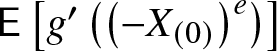 $\mathsf{E}\left[g'\left(\left(-X_{(0)}\right)^e\right)\right]$ are finite, then
  $\mathsf{E}[g(X)]$ is finite and
 \begin{equation}
\mathsf{E}[g(X)]=g(0)+\mu^+\mathsf{E}\left[g'\left(X_0^e\right)\right]-\mu^-\mathsf{E}\left[g'\left(\left(-X_{(0)}\right)^e\right)\right],
\end{equation}
\begin{equation}
\mathsf{E}[g(X)]=g(0)+\mu^+\mathsf{E}\left[g'\left(X_0^e\right)\right]-\mu^-\mathsf{E}\left[g'\left(\left(-X_{(0)}\right)^e\right)\right],
\end{equation} where  $\mu^+,\mu^-\in\mathbb{R}$ are defined as in Eq. (2.2).
Proof. The PDF of X can be written as
 \begin{equation*}
f(t)=pf_{-}(t)+(1-p)f_{+}(t),\qquad t\in\mathbb{R},
\end{equation*}
\begin{equation*}
f(t)=pf_{-}(t)+(1-p)f_{+}(t),\qquad t\in\mathbb{R},
\end{equation*} where  $p=F(0)$ and
 \begin{equation*}
f_{-}(t)=\frac{f(t)\mathbb{1}_{[t\le0]}}p,\quad f_{+}(t)=\frac{f(t)\mathbb{1}_{[t \gt 0]}}{1-p},\qquad t\in\mathbb{R},
\end{equation*}
\begin{equation*}
f_{-}(t)=\frac{f(t)\mathbb{1}_{[t\le0]}}p,\quad f_{+}(t)=\frac{f(t)\mathbb{1}_{[t \gt 0]}}{1-p},\qquad t\in\mathbb{R},
\end{equation*} are, respectively, the PDFs of 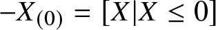 $-X_{(0)}=\left[X|X\le0\right]$ and
 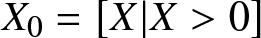 $X_0=\left[X|X \gt 0\right]$. Therefore, with a few calculations, one has
 \begin{align*}
\mathsf{E}[g(X)]&=p\,\mathsf{E}\left[g\left(-X_{(0)}\right)\right]+(1-p)\mathsf{E}[g(X_0)]\\
&=g(0)-p\,\mathsf{E}\left[X_{(0)}\right]\mathsf{E}\left[g'\left(\left(-X_{(0)}\right)^e\right)\right]+(1-p)\mathsf{E}\left[X_0\right]\mathsf{E}[g'(X_0^e)],
\end{align*}
\begin{align*}
\mathsf{E}[g(X)]&=p\,\mathsf{E}\left[g\left(-X_{(0)}\right)\right]+(1-p)\mathsf{E}[g(X_0)]\\
&=g(0)-p\,\mathsf{E}\left[X_{(0)}\right]\mathsf{E}\left[g'\left(\left(-X_{(0)}\right)^e\right)\right]+(1-p)\mathsf{E}\left[X_0\right]\mathsf{E}[g'(X_0^e)],
\end{align*} where in the last equality we have applied Theorem 3.2 to  $-X_{(0)}$ and Theorem 2.1 to X0. Since
 \begin{equation*}
\mathsf{E}\left[X_{(0)}\right]=\int_{-\infty}^{0}\int_{-\infty}^{t}f_{-}(x){\rm d}x{\rm d}t=\frac{\mu^-}{p},
\end{equation*}
\begin{equation*}
\mathsf{E}\left[X_{(0)}\right]=\int_{-\infty}^{0}\int_{-\infty}^{t}f_{-}(x){\rm d}x{\rm d}t=\frac{\mu^-}{p},
\end{equation*}and
 \begin{equation*}
\mathsf{E}\left[X_0\right]=\int_{0}^{+\infty}\int_{t}^{+\infty}f_{+}(x){\rm d}x{\rm d}t=\frac{\mu^+}{1-p},
\end{equation*}
\begin{equation*}
\mathsf{E}\left[X_0\right]=\int_{0}^{+\infty}\int_{t}^{+\infty}f_{+}(x){\rm d}x{\rm d}t=\frac{\mu^+}{1-p},
\end{equation*}then Eq. (3.4) is obtained. This completes the proof.
Corollary 3.1. Under the assumptions of Theorem 3.3, if g(t) is strictly convex for  $t\in\mathbb{R}$, having its minimum in t = 0, then
 \begin{equation*}
\mathsf{E}\left[g(X)\right]=g(0)+\mathsf{E}\left[|X|\right]\mathsf{E}\left[|g'\left(X^e\right)|\right].
\end{equation*}
\begin{equation*}
\mathsf{E}\left[g(X)\right]=g(0)+\mathsf{E}\left[|X|\right]\mathsf{E}\left[|g'\left(X^e\right)|\right].
\end{equation*}Proof. From Eq. (3.4), with straightforward calculations one has
 \begin{equation*}
\begin{aligned}
\mathsf{E}[g(X)]&=g(0)+\int_{0}^{+\infty}g'(t)\overline{F}(t){\rm d}t-\int_{-\infty}^{0}g'(t)F(t){\rm d}t\\
&=g(0)+\tilde{\mu}\left[\int_{0}^{+\infty}g'(t)f^e(t){\rm d}t-\int_{-\infty}^{0}g'(t)f^e(t){\rm d}t\right]\\
&=g(0)+\tilde{\mu}\left[\mathsf{E}\left[\left(g'\left(X^e\right)\right)^+\right]+\mathsf{E}\left[\left(g'\left(X^e\right)\right)^-\right]\right],
\end{aligned}
\end{equation*}
\begin{equation*}
\begin{aligned}
\mathsf{E}[g(X)]&=g(0)+\int_{0}^{+\infty}g'(t)\overline{F}(t){\rm d}t-\int_{-\infty}^{0}g'(t)F(t){\rm d}t\\
&=g(0)+\tilde{\mu}\left[\int_{0}^{+\infty}g'(t)f^e(t){\rm d}t-\int_{-\infty}^{0}g'(t)f^e(t){\rm d}t\right]\\
&=g(0)+\tilde{\mu}\left[\mathsf{E}\left[\left(g'\left(X^e\right)\right)^+\right]+\mathsf{E}\left[\left(g'\left(X^e\right)\right)^-\right]\right],
\end{aligned}
\end{equation*} where the last equality is obtained from Eq. (2.2) since, under the stated assumptions, g′ is invertible and such that  $g'(t)\le 0$ for all
  $t\le 0$ and
  $g'(t)\ge 0$ for all
  $t\ge 0$. Finally, the result follows by recalling Eq. (2.4).
4. Stochastic comparisons and aging properties
This section is devoted to investigate how stochastic orderings and aging properties are preserved through generalized equilibrium transformations, by taking into account the implications given in Tables 1 and 2, respectively. Distortion-based conditions for likelihood ratio comparisons between two generalized equilibrium random variables are included as well.
First we provide several results regarding stochastic comparisons. More in detail, we prove that many ordering conditions between baseline distributions are preserved by the corresponding generalized equilibrium distributions (sometimes by getting a stronger order).
Proposition 4.1. If  $X\le_{hr}Y$ and
  $X\le_{rhr}Y$, then
  $X^e\le_{lr}Y^e$.
Proof. By recalling Eq. (3.1), under the stated assumptions, one has  $F_X(0)\geq F_Y(0)$ and the likelihood ratio function
 \begin{equation*}
\frac{f^e_X(t)}{f^e_Y(t)}=
\begin{cases}
\displaystyle\frac{\tilde{\mu}_Y}{\tilde{\mu}_X}\,\frac{F_X(t)}{F_Y(t)},& t \lt 0, \\[3mm]
\displaystyle\frac{\tilde{\mu}_Y}{\tilde{\mu}_X}\,\frac{\overline{F}_X(t)}{\overline{F}_Y(t)},& t\ge0, \\
\end{cases}
\end{equation*}
\begin{equation*}
\frac{f^e_X(t)}{f^e_Y(t)}=
\begin{cases}
\displaystyle\frac{\tilde{\mu}_Y}{\tilde{\mu}_X}\,\frac{F_X(t)}{F_Y(t)},& t \lt 0, \\[3mm]
\displaystyle\frac{\tilde{\mu}_Y}{\tilde{\mu}_X}\,\frac{\overline{F}_X(t)}{\overline{F}_Y(t)},& t\ge0, \\
\end{cases}
\end{equation*} is decreasing in t, that is  $X^e\le_{lr}Y^e$.
From Proposition 4.1 and from the implications given in Table 1, below we show that the likelihood ratio order between two random variables is preserved by the corresponding generalized equilibrium ones. The same happens for the hazard rate and reversed hazard rate orders, when both hold.
Corollary 4.1. Let X and Y be random variables.
• If
$X\le_{hr}Y$ and
$X\le_{rhr}Y$, then
$X^e\le_{hr}Y^e$ and
$X^e\le_{rhr}Y^e$.• If X and Y have absolutely continuous distributions and
$X\le_{lr}Y$, then
$X^e\le_{lr}Y^e$.


If Y has distorted CDF from the one of X, then the likelihood ratio order between the corresponding generalized equilibrium random variables does not depend on the distribution of X, as shown below.
Theorem 4.1. Let X and Y be random variables having absolutely continuous distributions and such that the CDF of Y is distorted from the one of X, through a differentiable distortion function  $q$. Let us denote with
  $\tilde{q}$ the dual distortion function. Then anyone of the following statements implies
  $X^e\le_{lr}Y^e$:
(i)
$\tilde{q}(u)/u$ is decreasing in
$u\in(0,1]$ and
$q(u)/u$ is increasing in
$u\in(0,1]$;(ii)
$q$ is convex.


Proof. Regarding the assertion (i), the ratio  $\tilde{q}(u)/u$ is decreasing for
  $u\in(0,1]$ iff
  $X\le_{hr}Y$, while
  $q(u)/u$ is increasing for
  $u\in(0,1]$ iff
  $X\le_{rhr}Y$ (cf. Proposition 2 in Navarro et al. [Reference Navarro, Durante and Fernández-Sánchez23]). Then, the result follows from Proposition 4.1. Moreover, with a few calculations, when (ii) holds, then
  $X\le_{lr}Y$, and the thesis follows from Corollary 4.1.
Example 4.1. Let X be a random variable uniformly distributed in  $(-1,1)$, with CDF
  $F_X(t)=(t+1)/2$, for
  $t\in(-1,1)$. Let us assume that Y has distorted CDF
  $F_Y=q_{\alpha,\beta}(F_X)$, where
 \begin{equation}
q_{\alpha,\beta}(u)=\frac12 u^{\alpha}+\frac12 u^{\beta},\qquad u\in[0,1],
\end{equation}
\begin{equation}
q_{\alpha,\beta}(u)=\frac12 u^{\alpha}+\frac12 u^{\beta},\qquad u\in[0,1],
\end{equation} is a convex distortion function for  $\alpha,\beta \gt 1$, as shown in the LHS of Figure 1 for suitable choices of α and β. Hence, from (ii) of Theorem 4.1, it follows
  $X^e\le_{lr}Y^e$. Indeed, from Eq. (3.1) and by denoting with
  $c_{\alpha,\beta}=(\alpha+1)(\beta+1)/[2^{\alpha+\beta}(\alpha\beta-1)+2^\beta(\beta+1)+2^\alpha(\alpha+1)]$, the likelihood ratio function
 \begin{equation}
\frac{f^e_Y(t)}{f^e_X(t)}=
\begin{cases}
\displaystyle c_{\alpha,\beta}\left[2^{\beta-1}(t+1)^{\alpha-1}+2^{\alpha-1}(t+1)^{\beta-1}\right],& t\in(-1,0), \\
\displaystyle c_{\alpha,\beta}\frac{2^{\alpha+\beta}-2^{\beta-1}(t+1)^\alpha-2^{\alpha-1}(t+1)^\beta}{1-t},& t\in[0,1), \\
\end{cases}
\end{equation}
\begin{equation}
\frac{f^e_Y(t)}{f^e_X(t)}=
\begin{cases}
\displaystyle c_{\alpha,\beta}\left[2^{\beta-1}(t+1)^{\alpha-1}+2^{\alpha-1}(t+1)^{\beta-1}\right],& t\in(-1,0), \\
\displaystyle c_{\alpha,\beta}\frac{2^{\alpha+\beta}-2^{\beta-1}(t+1)^\alpha-2^{\alpha-1}(t+1)^\beta}{1-t},& t\in[0,1), \\
\end{cases}
\end{equation} is increasing in  $t\in(-1,1)$, as depicted in the RHS of Figure 1 for some choices of α and β.
Note that, if  $\alpha=\beta$, then the distortion given in Eq. (4.1) leads to the PRHR model.

Below we obtain sufficient ordering conditions on baseline distributions aiming to compare in the hazard rate order the corresponding generalized equilibrium distributions.
Proposition 4.2. If  $X\le_{mrl}Y$,
  $X\le_{mit}Y$,
  $Y^-\le_{st}X^-$ and
  $\tilde{\mu}_X\le\tilde{\mu}_Y$, then
  $X^e\le_{hr}Y^e$.
Proof. Let us denote with ζX and ζY the MRL functions of X and Y, while with  $\tilde{\zeta}_X$ and
  $\tilde{\zeta}_Y$ their MIT functions, respectively. Recalling Eq. (3.1), by adding and subtracting
  $\int_{-\infty}^{t}F_X(x){\rm d}x$ for t < 0, the HR of Xe becomes
 \begin{equation*}
\lambda_X^{e}(t)=
\begin{cases}
\displaystyle\left[\frac{\tilde{\mu}_X}{F_X(t)}-\tilde{\zeta}_X(t)\right]^{-1},& t \lt 0, \\[3mm]
\displaystyle\left[\zeta_X(t)\right]^{-1},& t\ge0.\\
\end{cases}
\end{equation*}
\begin{equation*}
\lambda_X^{e}(t)=
\begin{cases}
\displaystyle\left[\frac{\tilde{\mu}_X}{F_X(t)}-\tilde{\zeta}_X(t)\right]^{-1},& t \lt 0, \\[3mm]
\displaystyle\left[\zeta_X(t)\right]^{-1},& t\ge0.\\
\end{cases}
\end{equation*}With similar calculations, the HR of Ye can be expressed as
 \begin{equation*}
\lambda_Y^{e}(t)=
\begin{cases}
\displaystyle\left[\frac{\tilde{\mu}_Y}{F_Y(t)}-\tilde{\zeta}_Y(t)\right]^{-1},& t \lt 0, \\[3mm]
\displaystyle\left[\zeta_Y(t)\right]^{-1},& t\ge0.\\
\end{cases}
\end{equation*}
\begin{equation*}
\lambda_Y^{e}(t)=
\begin{cases}
\displaystyle\left[\frac{\tilde{\mu}_Y}{F_Y(t)}-\tilde{\zeta}_Y(t)\right]^{-1},& t \lt 0, \\[3mm]
\displaystyle\left[\zeta_Y(t)\right]^{-1},& t\ge0.\\
\end{cases}
\end{equation*} Therefore, if  $X\le_{mrl}Y$, then
  $\lambda_X^{e}(t)\ge\lambda_Y^{e}(t)$ for all
  $t\ge 0$. Moreover, since
  $Y^-\le_{st}X^-$ one has
  $F_X(t)\ge F_Y(t)$ for all t < 0. Hence, under the condition
  $\tilde{\mu}_X\le\tilde{\mu}_Y$, if
  $X\le_{mit}Y$, then
  $\lambda_X^{e}(t)\ge\lambda_Y^{e}(t)$ also holds for all t < 0, and the thesis follows.
Let us consider an example that satisfies the assumptions of Proposition 4.2.
Example 4.2. Let X be uniformly distributed in  $(-1,1/2)$, with CDF
  $F_X(t)=2(t+1)/3$, for
  $t\in(-1,1/2)$. Let Y be uniformly distributed in
  $(-1,1)$, having CDF
  $F_Y(t)=(t+1)/2$, for
  $t\in(-1,1)$. The likelihood ratio function
 \begin{equation*}
\frac{f_X(t)}{f_Y(t)}=
\begin{cases}
\displaystyle \frac43,& t\in(-1,\frac12], \\[3mm]
\displaystyle 0,& t\in(\frac12,1),\\
\end{cases}
\end{equation*}
\begin{equation*}
\frac{f_X(t)}{f_Y(t)}=
\begin{cases}
\displaystyle \frac43,& t\in(-1,\frac12], \\[3mm]
\displaystyle 0,& t\in(\frac12,1),\\
\end{cases}
\end{equation*} is decreasing in t, that is  $X\le_{lr}Y$. Then, from Table 1, one has
  $X\le_{mrl}Y$ and
  $X\le_{mit}Y$. From Eq. (2.1), one gets
  $Y^-\le_{st}X^-$. By recalling Eq. (2.4), it holds
  $5/12=\tilde{\mu}_X \lt \tilde{\mu}_Y=1/2$. Hence, by applying Proposition 4.2, it follows
  $X^e\le_{hr}Y^e$.
An analogous result to Proposition 4.2 holds for the reversed hazard rate order.
Proposition 4.3. If  $X\le_{mrl}Y$,
  $X\le_{mit}Y$,
  $X^+\le_{st}Y^+$ and
  $\tilde{\mu}_X\ge\tilde{\mu}_Y$, then
  $X^e\le_{rhr}Y^e$.
Proof. Let us denote with ζX and ζY the MRL of X and Y, while with  $\tilde{\zeta}_X$ and
  $\tilde{\zeta}_Y$ their MIT, respectively. Recalling Eq. (3.1), by adding and subtracting
  $\int_{t}^{+\infty}\overline{F}_X(x){\rm d}x$ for
  $t\ge0$, the RHR of Xe becomes
 \begin{equation*}
\tau_X^{e}(t)=
\begin{cases}
\displaystyle\left[\tilde\zeta_X(t)\right]^{-1},& t \lt 0, \\[3mm]
\displaystyle\left[\frac{\tilde{\mu}_X}{\overline{F}_X(t)}-\zeta_X(t)\right]^{-1} ,& t\ge0\\
\end{cases}
\end{equation*}
\begin{equation*}
\tau_X^{e}(t)=
\begin{cases}
\displaystyle\left[\tilde\zeta_X(t)\right]^{-1},& t \lt 0, \\[3mm]
\displaystyle\left[\frac{\tilde{\mu}_X}{\overline{F}_X(t)}-\zeta_X(t)\right]^{-1} ,& t\ge0\\
\end{cases}
\end{equation*} and similarly for the RHR  $\tau_Y^{e}$ of Ye. Hence, if
  $X\le_{mit}Y$, then
  $\tau_X^{e}(t)\le\tau_Y^{e}(t)$ for all t < 0. In addition,
  $X^+\le_{st}Y^+$ implies
  $\overline{F}_X(t)\le\overline{F}_Y(t)$ for all
  $t\ge 0$. Therefore, under the condition
  $\tilde{\mu}_X\ge\tilde{\mu}_Y$, if
  $X\le_{mrl}Y$, then
  $\tau_X^{e}(t)\le\tau_Y^{e}(t)$ also holds for all
  $t\ge 0$. This completes the proof.
The random variables in the following example satisfy the conditions of Proposition 4.3.
Example 4.3. Let X be uniformly distributed in  $(-1,1)$, with CDF
  $F_X(t)=(t+1)/2$, for
  $t\in(-1,1)$. Let Y be standard uniformly distributed. The likelihood ratio function
 \begin{equation*}
\frac{f_X(t)}{f_Y(t)}=
\begin{cases}
\displaystyle +\infty,& t\in(-1,0), \\[3mm]
\displaystyle \frac12,& t\in[0,1),\\
\end{cases}
\end{equation*}
\begin{equation*}
\frac{f_X(t)}{f_Y(t)}=
\begin{cases}
\displaystyle +\infty,& t\in(-1,0), \\[3mm]
\displaystyle \frac12,& t\in[0,1),\\
\end{cases}
\end{equation*} is decreasing in t, that is  $X\le_{lr}Y$. Then, from Table 1, one has
  $X\le_{mrl}Y$ and
  $X\le_{mit}Y$. From Eq. (2.1), one gets
  $X^+\le_{st}Y^+$. By recalling Eq. (2.4), it holds
  $\tilde{\mu}_X=\tilde{\mu}_Y=1/2$. Hence, by applying Proposition 4.3, it follows
  $X^e\le_{rhr}Y^e$.
By combining Propositions 4.2 and 4.3 we get the next result.
Corollary 4.2. Let X and Y be random variables such that  $X\le_{st}Y$ and
  $\tilde{\mu}_X=\tilde{\mu}_Y$.
• If
$X\le_{mrl}Y$ and
$X\le_{mit}Y$, then
$X^e\le_{hr}Y^e$ and
$X^e\le_{rhr}Y^e$


and therefore
• If
$X\le_{mrl}Y$ and
$X\le_{mit}Y$, then
$X^e\le_{mrl}Y^e$ and
$X^e\le_{mit}Y^e$.

In the following, we obtain sufficient conditions on the baseline distributions in order to compare in the usual stochastic order the corresponding generalized equilibrium distributions.
Proposition 4.4. If  $X\le_{icx}Y$,
  $X\le_{icv}Y$ and
  $\tilde{\mu}_X=\tilde{\mu}_Y$, then
  $X^e\le_{st}Y^e$.
Proof. Let us denote  $\tilde{\mu}_X=\tilde{\mu}_Y=\tilde{\mu}$. From Eq. (3.1), the SF of Xe can be expressed as
 \begin{equation}
\overline{F}_X^{e}(t)=
\begin{cases}
\displaystyle1-\frac1{\tilde{\mu}}\int_{-\infty}^{t}F_X(s){\rm d}s,& t \lt 0, \\[3mm]
\displaystyle\frac1{\tilde{\mu}}\int_{t}^{+\infty}\overline{F}_X(s){\rm d}s,& t\ge0\\
\end{cases}
\end{equation}
\begin{equation}
\overline{F}_X^{e}(t)=
\begin{cases}
\displaystyle1-\frac1{\tilde{\mu}}\int_{-\infty}^{t}F_X(s){\rm d}s,& t \lt 0, \\[3mm]
\displaystyle\frac1{\tilde{\mu}}\int_{t}^{+\infty}\overline{F}_X(s){\rm d}s,& t\ge0\\
\end{cases}
\end{equation} and similarly for the SF  $\overline{F}_Y^{e}$ of Ye. Hence, if
  $X\le_{icx}Y$, then
  $\overline{F}_X^{e}(t)\le\overline{F}_Y^e(t)$ for all
  $t\ge 0$, and since
  $X\le_{icv}Y$, it follows
  $\overline{F}_X^{e}(t)\le\overline{F}_Y^e(t)$ also for all t < 0. This concludes the proof.
Note that in Proposition 4.4 the assumption  $X\le_{icv}Y$ can be replaced by
  $X^-\le_{st}Y^-$.
Proposition 4.5. If  $X\le_{cx}Y$ and
  $\mu^-_X=\mu^-_Y$, then
  $(X^e)^-\le_{st}(Y^e)^-$ and
  $(X^e)^+\le_{st}(Y^e)^+$.
Proof. If  $X\le_{cx}Y$, then
  $\mu_X=\mu_Y$. Therefore, by recalling Eqs. (2.3) and (2.4), if
  $\mu^-_X=\mu^-_Y$, then
  $\tilde{\mu}_X=\tilde{\mu}_Y=\tilde{\mu}$. Hence, from Eq. (4.3), since
  $X\le_{cx}Y$, then
  $\overline{F}_X^{e}(t)\ge(\le)\overline{F}_Y^{e}(t)$ for all
  $t \lt (\ge)0$. The thesis follows by recalling Eq. (2.1).
Hereafter, we obtain a sufficient condition for which the usual stochastic order is preserved under generalized equilibrium transformations.
Proposition 4.6. Let X and Y be random variables such that  $\tilde{\mu}_X=\tilde{\mu}_Y$. If
  $X\le_{st}Y$, then
  $X^e\le_{st}Y^e$.
Proof. From Eq. (3.1), if  $\tilde{\mu}_X=\tilde{\mu}_Y$ and
  $X\le_{st}Y$, then
  $f^e_X(t)\ge f^e_Y(t)$ for all
  $t\le0$ and
  $f^e_X(t)\le f^e_Y(t)$ for all
  $t\ge0$. Hence, the thesis follows from Lemma 2.2 in Kochar [Reference Kochar16].
Below we obtain aging conditions on a given random variable aiming to perform likelihood ratio comparisons with its generalized equilibrium version.
Proposition 4.7. Let X be a random variable with absolutely continuous distribution having support containing 0 and with median  $m\ge0$. If X is DFR, then
  $X\le_{lr}X^{e}$.
Proof. Let us denote with f, λ and τ the PDF, HR and RHR of X, respectively. If X is DFR, then it is DRFR (cf. Table 2). Moreover, since  $m\ge0$, then
  $F(0)\leq 1/2$ and one has
 \begin{equation*}
\tau(0)-\lambda(0)=\tau(0)\, \frac{1-2\,F(0)}{\overline F(0)}\geq 0.
\end{equation*}
\begin{equation*}
\tau(0)-\lambda(0)=\tau(0)\, \frac{1-2\,F(0)}{\overline F(0)}\geq 0.
\end{equation*}Hence, from Eq. (3.1) and the DFR and DRFR properties, the ratio
 \begin{equation*}
\frac{f(t)}{f^{e}(t)}=
\begin{cases}
\displaystyle\tilde{\mu}\,\tau(t),& t \lt 0, \\
\displaystyle\tilde{\mu}\,\lambda(t),& t\ge0, \\
\end{cases}
\end{equation*}
\begin{equation*}
\frac{f(t)}{f^{e}(t)}=
\begin{cases}
\displaystyle\tilde{\mu}\,\tau(t),& t \lt 0, \\
\displaystyle\tilde{\mu}\,\lambda(t),& t\ge0, \\
\end{cases}
\end{equation*} is decreasing in t, i.e.,  $X\le_{lr}X^{e}$.
We now provide further results involving aging notions. More in detail, we prove that some aging classes are preserved through generalized equilibrium transformations. Note that, from Remark 3.1, Xe cannot be DFR in  $\mathbb{R}$ since its HR is always increasing for
  $t\in(-\infty,0)$.
Proposition 4.8. Let X be a random variable with absolutely continuous distribution. If X is IFR and DRFR, then Xe is ILR.
Proof. Let us denote with f the PDF of X. From Eq. (3.1) one has
 \begin{equation*}
\frac{\rm{d}}{\rm{d}t}f^e(t)=
\begin{cases}
\displaystyle\frac{f(t)}{\tilde{\mu}},& t \lt 0, \\[3mm]
\displaystyle-\frac{f(t)}{\tilde{\mu}},& t\ge0 \\
\end{cases}
\end{equation*}
\begin{equation*}
\frac{\rm{d}}{\rm{d}t}f^e(t)=
\begin{cases}
\displaystyle\frac{f(t)}{\tilde{\mu}},& t \lt 0, \\[3mm]
\displaystyle-\frac{f(t)}{\tilde{\mu}},& t\ge0 \\
\end{cases}
\end{equation*}and therefore Glaser’s function of Xe is
 \begin{equation*}
\eta^e(t)=
\begin{cases}
\displaystyle-\tau(t),& t \lt 0, \\[3mm]
\displaystyle\lambda(t),& t\ge0, \\
\end{cases}
\end{equation*}
\begin{equation*}
\eta^e(t)=
\begin{cases}
\displaystyle-\tau(t),& t \lt 0, \\[3mm]
\displaystyle\lambda(t),& t\ge0, \\
\end{cases}
\end{equation*} where λ and τ denote the HR and RHR of X, respectively. Hence, since  $\eta^e(0^+)-\eta^e(0^-)=\lambda(0^+)+\tau(0^-)\ge0$, if X is IFR and DRFR, then
  $\eta^e(t)$ is increasing in t. This completes the proof.
In the following, from Proposition 4.8 and from the implications given in Table 2, we show that the generalized equilibrium distribution preserves the ILR property of the baseline random variable. The same for IFR and DRFR properties, whenever they hold simultaneously.
Corollary 4.3. Let X be a random variable with absolutely continuous distribution.
• If X is ILR, then Xe is ILR.
• If X is IFR and DRFR, then Xe is IFR and DRFR.
Hereafter, we provide further aging results under suitable assumptions on the median of the baseline distribution.
Proposition 4.9. Let X be a random variable with median m.
(i) If
$m\ge0$ and X is DMRL, then Xe is IFR.(ii) If
$m\le0$ and X is IMIT, then Xe is DRFR.

Proof. Making use of Eq. (3.1), by denoting with ζ the MRL of X, the HR of Xe
 \begin{equation*}
\lambda^{e}(t)=
\begin{cases}
\displaystyle\frac{F(t)}{\int_{t}^{0}F(x){\rm d}x+\mu^{+}},& t \lt 0, \\[3mm]
\displaystyle\left[\zeta(t)\right]^{-1},& t\ge0, \\
\end{cases}
\end{equation*}
\begin{equation*}
\lambda^{e}(t)=
\begin{cases}
\displaystyle\frac{F(t)}{\int_{t}^{0}F(x){\rm d}x+\mu^{+}},& t \lt 0, \\[3mm]
\displaystyle\left[\zeta(t)\right]^{-1},& t\ge0, \\
\end{cases}
\end{equation*} is increasing for t < 0. If X is DMRL, then  $\lambda^{e}(t)$ is also increasing for
  $t\ge0$. If
  $m\ge0$, then
 \begin{equation*}
\lambda^{e}(0^+)-\lambda^{e}(0^-)=\frac{\overline{F}(0)-F(0^-)}{\mu^{+}}\ge0
\end{equation*}
\begin{equation*}
\lambda^{e}(0^+)-\lambda^{e}(0^-)=\frac{\overline{F}(0)-F(0^-)}{\mu^{+}}\ge0
\end{equation*} and the statement (i) follows. Similarly, from Eq. (3.1), by denoting with  $\tilde{\zeta}$ the MIT of X, the RHR of Xe
 \begin{equation*}
\tau^{e}(t)=
\begin{cases}
\displaystyle\left[\tilde{\zeta}(t)\right]^{-1},& t \lt 0, \\[3mm]
\displaystyle\frac{\overline{F}(t)}{\mu^{-}+\int_{0}^{t}\overline{F}(x){\rm d}x},& t\ge0, \\
\end{cases}
\end{equation*}
\begin{equation*}
\tau^{e}(t)=
\begin{cases}
\displaystyle\left[\tilde{\zeta}(t)\right]^{-1},& t \lt 0, \\[3mm]
\displaystyle\frac{\overline{F}(t)}{\mu^{-}+\int_{0}^{t}\overline{F}(x){\rm d}x},& t\ge0, \\
\end{cases}
\end{equation*} is decreasing for  $t\ge0$ and if X is IMIT, then it is also decreasing for t < 0. If
  $m\le0$, then one has
 \begin{equation*}
\tau^{e}(0^+)-\tau^{e}(0^-)=\frac{\overline{F}(0)-F(0^-)}{\mu^{-}}\le0
\end{equation*}
\begin{equation*}
\tau^{e}(0^+)-\tau^{e}(0^-)=\frac{\overline{F}(0)-F(0^-)}{\mu^{-}}\le0
\end{equation*}and the statement (ii) follows. This concludes the proof.
If X is non-negative, then from Eq. (1.1) one has that Xe is IFR iff X is DMRL. However, the reverse implication in (i) of Proposition 4.9 does not hold in general. Indeed, if X has support  $\left[-1/2,+\infty\right)$ with the following SF
 \begin{equation*}
\overline{F}(t)=
\begin{cases}
\displaystyle\frac1{2+2t},& t\in\left[-\frac12,0\right], \\[3mm]
\displaystyle\frac{e^{-t}}{2},& t\ge0, \\
\end{cases}
\end{equation*}
\begin{equation*}
\overline{F}(t)=
\begin{cases}
\displaystyle\frac1{2+2t},& t\in\left[-\frac12,0\right], \\[3mm]
\displaystyle\frac{e^{-t}}{2},& t\ge0, \\
\end{cases}
\end{equation*}then its median is zero. A straightforward calculation shows that Xe is IFR but X is not DMRL.
By recalling the implications given in Table 2, from (i) of Proposition 4.9, the generalized equilibrium distribution maintains the IFR and DMRL properties of the original distribution. Similarly, the DRFR and IMIT properties are preserved according to (ii) of Proposition 4.9, as it is stated below.
Corollary 4.4. Let X be a random variable having median m.
• If
$m\ge0$ and X is IFR, then Xe is IFR.• If
$m\ge0$ and X is DMRL, then Xe is DMRL.• If
$m\le0$ and X is DRFR, then Xe is DRFR.• If
$m\le0$ and X is IMIT, then Xe is IMIT.


5. Equilibrium density of two ordered random variables
In this section, we study the equilibrium PDF of two ordered random variables that are not necessarily non-negative. In particular, we prove a probabilistic analog of the mean value theorem in the proposed case of study. We investigate conditions for the unimodality of this new equilibrium PDF. Further results are provided too, some of them regarding stochastic comparisons. In particular, for the likelihood ratio order, special attention is devoted to the case in which the involved random variables are connected through suitable distortion functions.
The following result extends Proposition 5.1 provided in Di Crescenzo [Reference Di Crescenzo11] for the case of non-negative random variables.
Proposition 5.1. Let X and Y be random variables such that  $-\infty \lt \mathsf{E}[X] \lt \mathsf{E}[Y] \lt +\infty$. Then
 \begin{equation}
f_Z(t)=\frac{\overline{F}_Y(t)-\overline{F}_X(t)}{\mathsf{E}[Y]-\mathsf{E}[X]}=\frac{F_X(t)-F_Y(t)}{\mathsf{E}[Y]-\mathsf{E}[X]},\qquad t\in\mathbb{R},
\end{equation}
\begin{equation}
f_Z(t)=\frac{\overline{F}_Y(t)-\overline{F}_X(t)}{\mathsf{E}[Y]-\mathsf{E}[X]}=\frac{F_X(t)-F_Y(t)}{\mathsf{E}[Y]-\mathsf{E}[X]},\qquad t\in\mathbb{R},
\end{equation} is the PDF of a random variable Z with an absolutely continuous distribution iff  $X\le_{st}Y$.
Proof. One has  $f_Z(t)\ge 0$, for all
  $t\in\mathbb{R}$, iff
  $X\le_{st}Y$. Moreover, from Eqs. (2.2) and (2.3) it follows
 \begin{equation*}
\begin{aligned}
\int_{-\infty}^{+\infty}f_Z(t){\rm d}t&=\int_{-\infty}^{0}\frac{F_X(t)-F_Y(t)}{\mathsf{E}[Y]-\mathsf{E}[X]}{\rm d}t+\int_{0}^{+\infty}\frac{\overline{F}_Y(t)-\overline{F}_X(t)}{\mathsf{E}[Y]-\mathsf{E}[X]}{\rm d}t\\
&=\frac{\mu^-_X-\mu^-_Y}{\mathsf{E}[Y]-\mathsf{E}[X]}+\frac{\mu^+_Y-\mu^+_X}{\mathsf{E}[Y]-\mathsf{E}[X]}=1
\end{aligned}
\end{equation*}
\begin{equation*}
\begin{aligned}
\int_{-\infty}^{+\infty}f_Z(t){\rm d}t&=\int_{-\infty}^{0}\frac{F_X(t)-F_Y(t)}{\mathsf{E}[Y]-\mathsf{E}[X]}{\rm d}t+\int_{0}^{+\infty}\frac{\overline{F}_Y(t)-\overline{F}_X(t)}{\mathsf{E}[Y]-\mathsf{E}[X]}{\rm d}t\\
&=\frac{\mu^-_X-\mu^-_Y}{\mathsf{E}[Y]-\mathsf{E}[X]}+\frac{\mu^+_Y-\mu^+_X}{\mathsf{E}[Y]-\mathsf{E}[X]}=1
\end{aligned}
\end{equation*}and this completes the proof.
Definition 5.1. Under the assumptions of Proposition 5.1, a random variable Z having absolutely continuous distribution according to the equilibrium PDF given in Eq. (5.1), is denoted as  $Z\equiv\Psi(X,Y)$.
We can connect  $Z\equiv\Psi(X,Y)$ with the generalized equilibrium distribution defined in Section 3. Indeed, if X and Y are non-negative (non-positive), then from Eq. (3.1) and Proposition 5.1 one has
 \begin{equation}
f_Z(t)=\frac{\mathsf{E}[Y]}{\mathsf{E}[Y]-\mathsf{E}[X]}f^e_Y(t)-\frac{\mathsf{E}[X]}{\mathsf{E}[Y]-\mathsf{E}[X]}f^e_X(t),\qquad t\ge(\le) 0
\end{equation}
\begin{equation}
f_Z(t)=\frac{\mathsf{E}[Y]}{\mathsf{E}[Y]-\mathsf{E}[X]}f^e_Y(t)-\frac{\mathsf{E}[X]}{\mathsf{E}[Y]-\mathsf{E}[X]}f^e_X(t),\qquad t\ge(\le) 0
\end{equation} and therefore fZ is a generalized mixture between  $f^e_X$ and
  $f^e_Y$. We recall that the generalized mixtures are defined as the classic ones but they might contain negative coefficients, as in Eq. (5.2). Note that, if X is non-positive and Y is non-negative, then Eq. (5.2) holds again, and in this case fZ is a classical mixture between
  $f^e_X$ and
  $f^e_Y$. Hence, in all the mentioned cases, FZ,
  $\overline{F}_Z$,
  $\mathsf{E}(Z)$ and other moments of Z can be also obtained from the ones of Xe and Ye by using Eq. (5.2).
Remark 5.1. Let X and Y be non-negative (non-positive) random variables, such that  $X\le_{st}Y$. From Eq. (5.2), by setting
  $p=\mathsf{E}[X]/\mathsf{E}[Y]\in(0,1)$, it follows
 \begin{equation*}
f^e_Y(t)=pf^e_X(t)+(1-p)f_{Z}(t),\qquad t\ge(\le) 0,
\end{equation*}
\begin{equation*}
f^e_Y(t)=pf^e_X(t)+(1-p)f_{Z}(t),\qquad t\ge(\le) 0,
\end{equation*} i.e.,  $f^e_Y$ is a mixture between
  $f^e_X$ and fZ, and therefore
  $f^e_Y$ takes values between
  $f^e_X$ and fZ.
Recently, the bivariate Gini’s mean difference has been defined and studied in Capaldo and Navarro [Reference Capaldo and Navarro6]. The formal definition is stated as follows.
Definition 5.2. Let (X, Y) be a random vector. The bivariate Gini’s mean difference of (X, Y) is defined as
 \begin{equation}
\mathsf{GMD}(X,Y)=\mathsf{E}|X-Y|,
\end{equation}
\begin{equation}
\mathsf{GMD}(X,Y)=\mathsf{E}|X-Y|,
\end{equation}provided that X and Y have finite means.
Note that, while the bivariate Gini’s mean difference in Eq. (5.3) can measure the expected absolute distance between X and Y, the PDF of  $Z\equiv\Psi(X,Y)$ can measure the distance between the SFs of X and Y. Indeed, the PDF given in Eq. (5.1) is related with the Kolmogorov distance, which is defined for any pairs of random variables
  $X$ and Y as
 \begin{equation}
K(X,Y)=\sup_{t\in\mathbb{R}}|\overline{F}_Y(t)-\overline{F}_X(t)|,
\end{equation}
\begin{equation}
K(X,Y)=\sup_{t\in\mathbb{R}}|\overline{F}_Y(t)-\overline{F}_X(t)|,
\end{equation}see, for instance, Denuit et al. [Reference Denuit, Dhaene, Goovaerts and Kaas9], p. 396.
Remark 5.2. We recall that  $X\le_{st}Y$ iff there exist two random variables
  $\tilde{X}$ and
  $\tilde{Y}$ defined on the same probability space, such that
  $X=_{st}\tilde{X}$,
  $Y=_{st}\tilde{Y}$ and
  $\mathsf{P}\left(\tilde{X}\le \tilde{Y}\right)=1$ (see Theorem 1.A.1 in Shaked and Shanthikumar [Reference Shaked and Shanthikumar31]). Therefore, from Eqs. (5.1) and (5.3), one has
 \begin{equation*}
f_Z(t)=\frac{\overline{F}_Y(t)-\overline{F}_X(t)}{\mathsf{GMD}(\tilde{X},\tilde{Y})},\qquad t\ge 0.
\end{equation*}
\begin{equation*}
f_Z(t)=\frac{\overline{F}_Y(t)-\overline{F}_X(t)}{\mathsf{GMD}(\tilde{X},\tilde{Y})},\qquad t\ge 0.
\end{equation*}The following result extends Proposition 3.3 in Di Crescenzo [Reference Di Crescenzo11], given for non-negative random variables, to the case of general supports. Hence, the proof is omitted for brevity.
Proposition 5.2. Let X and Y be random variables such that  $X\le_{st}Y$ and
  $-\infty \lt \mathsf{E}[X] \lt \mathsf{E}[Y] \lt +\infty$. Let W be a random variable with finite mean, independent from
  $X$ and
  $Y$. Then, it follows
 \begin{equation*}
\Psi(X,Y)+W=_{st}\Psi(X+W,Y+W).
\end{equation*}
\begin{equation*}
\Psi(X,Y)+W=_{st}\Psi(X+W,Y+W).
\end{equation*}Hereafter, by using Theorem 3.3, we prove a probabilistic version of the mean value theorem in our case of study.
Theorem 5.1. Let X and Y be random variables such that  $X\le_{st}Y$ and
  $-\infty \lt \mathsf{E}[X] \lt \mathsf{E}[Y] \lt +\infty$. Let
  $Z\equiv\Psi(X,Y)$. Let
  $g:\mathbb{R}\rightarrow\mathbb{R}$ be a measurable and differentiable function such that
  $\mathsf{E}[g(X)]$ and
  $\mathsf{E}[g(Y)]$ are finite, and let its derivative g′ be measurable and Riemann-integrable. Then
  $\mathsf{E}[g'(Z)]$ is finite and
 \begin{equation}
\mathsf{E}[g'(Z)]=\frac{\mathsf{E}[g(Y)]-\mathsf{E}[g(X)]}{\mathsf{E}[Y]-\mathsf{E}[X]}.
\end{equation}
\begin{equation}
\mathsf{E}[g'(Z)]=\frac{\mathsf{E}[g(Y)]-\mathsf{E}[g(X)]}{\mathsf{E}[Y]-\mathsf{E}[X]}.
\end{equation}Proof. From Eq. (3.4) with straightforward calculations one has
 \begin{equation*}
\mathsf{E}[g(X)]=g(0)+\int_{0}^{+\infty}g'(t)\overline{F}_X(t){\rm d}t-\int_{-\infty}^{0}g'(t)F_X(t){\rm d}t
\end{equation*}
\begin{equation*}
\mathsf{E}[g(X)]=g(0)+\int_{0}^{+\infty}g'(t)\overline{F}_X(t){\rm d}t-\int_{-\infty}^{0}g'(t)F_X(t){\rm d}t
\end{equation*} and similarly for  $\mathsf{E}[g(Y)]$. Therefore, by recalling Eq. (5.1), it follows
 \begin{equation*}
\begin{aligned}
\mathsf{E}[g(Y)]-\mathsf{E}[g(X)]&=\int_{0}^{+\infty}g'(t)\left[\overline{F}_Y(t)-\overline{F}_X(t)\right]{\rm d}t+\int_{-\infty}^{0}g'(t)\left[F_X(t)-F_Y(t)\right]{\rm d}t\\
&=\left\{\mathsf{E}[Y]-\mathsf{E}[X]\right\}\int_{-\infty}^{+\infty}g'(t)f_Z(t){\rm d}t
\end{aligned}
\end{equation*}
\begin{equation*}
\begin{aligned}
\mathsf{E}[g(Y)]-\mathsf{E}[g(X)]&=\int_{0}^{+\infty}g'(t)\left[\overline{F}_Y(t)-\overline{F}_X(t)\right]{\rm d}t+\int_{-\infty}^{0}g'(t)\left[F_X(t)-F_Y(t)\right]{\rm d}t\\
&=\left\{\mathsf{E}[Y]-\mathsf{E}[X]\right\}\int_{-\infty}^{+\infty}g'(t)f_Z(t){\rm d}t
\end{aligned}
\end{equation*}and the proof is completed.
Note that, if X and Y have absolutely continuous distributions, then Theorem 5.1 can be also proved by making use of integration by parts in the computation of  $\mathsf{E}[g'(Z)]$ and by using the following assumption
 \begin{equation*}
\lim_{t\to-\infty}g(t)\left[\overline{F}_Y(t)-\overline{F}_X(t)\right]=\lim_{t\to+\infty} g(t)\left[\overline{F}_Y(t)-\overline{F}_X(t)\right]=0,
\end{equation*}
\begin{equation*}
\lim_{t\to-\infty}g(t)\left[\overline{F}_Y(t)-\overline{F}_X(t)\right]=\lim_{t\to+\infty} g(t)\left[\overline{F}_Y(t)-\overline{F}_X(t)\right]=0,
\end{equation*} see Lemma 2.1 in Psarrakos [Reference Psarrakos28]. We also remark that, under appropriate assumptions, Di Crescenzo [Reference Di Crescenzo11] showed that Eq. (5.5) holds for non-negative random variables by using Theorem 2.1. Moreover, Proposition 4.1 in [Reference Di Crescenzo11] can be straightforwardly extended to the case of random variables having support in  $\mathbb{R}$ by using Theorem 5.1.
In the next result, we obtain conditions for which  $Z\equiv\Psi(X,Y)$ has median zero.
Proposition 5.3. Let X and Y be random variables such that  $X\le_{st}Y$ and
  $-\infty \lt \mathsf{E}[X] \lt \mathsf{E}[Y] \lt +\infty$. If
  $\tilde{\mu}_X=\tilde{\mu}_Y$, then
  $Z\equiv\Psi(X,Y)$ has median zero.
Proof. Recalling Eq. (2.4), if  $\tilde{\mu}_X=\tilde{\mu}_Y$, then
  $\mu^-_X-\mu^-_Y=\mu^+_Y-\mu^+_X$. Therefore, by using Eq. (5.1), it follows
 \begin{equation*}
\int_{-\infty}^{0}\frac{F_X(t)-F_Y(t)}{\mathsf{E}[Y]-\mathsf{E}[X]}{\rm d}t=\int_{0}^{+\infty}\frac{\overline{F}_Y(t)-\overline{F}_X(t)}{\mathsf{E}[Y]-\mathsf{E}[X]}{\rm d}t=\frac12
\end{equation*}
\begin{equation*}
\int_{-\infty}^{0}\frac{F_X(t)-F_Y(t)}{\mathsf{E}[Y]-\mathsf{E}[X]}{\rm d}t=\int_{0}^{+\infty}\frac{\overline{F}_Y(t)-\overline{F}_X(t)}{\mathsf{E}[Y]-\mathsf{E}[X]}{\rm d}t=\frac12
\end{equation*}and the proof is obtained.
We now provide various results regarding unimodality issues for the PDF of  $Z\equiv\Psi(X,Y)$. Note that, by recalling Eq. (5.4), if fZ is unimodal with mode
  $\nu$, then
  $K(X,Y)=f_Z(\nu)\{\mathsf{E}[Y]-\mathsf{E}[X]\}$.
Proposition 5.4. Let X be a non-positive random variable and let Y be a non-negative random variable, having CDFs denoted as  $F_X$ and
  $F_Y$, respectively. If
  $X\le_{st}Y$ and if there exists δ > 0 such that
  $F_X(t)$ is strictly increasing for
  $t\in(-\delta,0)$ and
  $F_Y(t)$ is strictly increasing for
  $t\in(0,\delta)$, then
  $Z\equiv\Psi(X,Y)$ has unimodal PDF with mode zero.
Proof. The result follows with a few calculations from Eq. (5.1).
Proposition 5.5. Let X and Y have absolutely continuous distributions and the same support, with continuous PDFs fX and fY, respectively. If X and Y satisfy the assumptions of Proposition 5.1, then the PDF fZ is unimodal, with mode t 0 iff t 0 is the unique solution of  $f_X(t)=f_Y(t)$.
Proof. Since X and Y have the same support, due to the continuity of fX and fY, then there exists  $t_0\in\mathbb{R}$ such that
  $f_X(t_0)=f_Y(t_0)$. Moreover, from Eq. (5.1), one has
 \begin{equation*}
f'_Z(t)=\frac{f_X(t)-f_Y(t)}{\mathsf{E}[Y]-\mathsf{E}[X]}=0
\end{equation*}
\begin{equation*}
f'_Z(t)=\frac{f_X(t)-f_Y(t)}{\mathsf{E}[Y]-\mathsf{E}[X]}=0
\end{equation*} and therefore the assertion (ii) follows iff t 0 is the unique solution of  $f_X(t)=f_Y(t)$.
By taking into account Lemma 2.2 in Kochar [Reference Kochar16] and Proposition 5.5, we can go a step further and prove the following result.
Proposition 5.6. Let X and Y have absolutely continuous distributions and the same support, with continuous PDFs  $f_X$ and
  $f_Y$, respectively. Let us assume that
  $-\infty \lt \mathsf{E}[X] \lt \mathsf{E}[Y] \lt +\infty$. If t 0 is the unique solution of
  $f_X(t)=f_Y(t)$, then
  $X\le_{st} Y$ and
  $f_Z$ is unimodal.
In the following remark, we assume a stronger condition than the usual stochastic order between the two random variables which lead to Z.
Remark 5.3. Under the assumptions of Proposition 5.5, if the ratio  $f_X(t)/f_Y(t)$ is strictly decreasing and continuous for
  $t\in\mathbb{R}$, then fZ is unimodal.
When Y has distorted CDF from the one of X through a suitable distortion function, then the conditions given in Proposition 5.5 for the unimodality of fZ can be characterized as follows.
Proposition 5.7. Let X be a random variable with support  $(l,u)\subset\mathbb{\overline{R}}$, having absolutely continuous CDF F and PDF f. Let Y have distorted CDF
  $F_Y=q(F)$ through the differentiable distortion function
  $q$. Let us assume
  $q(u)\le u$ for
  $u\in(0,1)$ and
  $-\infty \lt \mathsf{E}[X] \lt \mathsf{E}[Y] \lt +\infty$. If there exists a unique point
  $u_0\in(0,1)$ such that
  $q'(u_0)=1$, then
  $Z\equiv\Psi(X,Y)$ has a unimodal PDF fZ with mode
  $t_0=F^{-1}(u_0)$ iff F is strictly increasing around t 0.
Proof. Under the stated hypothesis, from Eq. (5.1) one has
 \begin{equation*}
f'_Z(t)=\frac{f(t)}{\mathsf{E}[Y]-\mathsf{E}[X]}\left\{1-q'(F(t))\right\}=0
\end{equation*}
\begin{equation*}
f'_Z(t)=\frac{f(t)}{\mathsf{E}[Y]-\mathsf{E}[X]}\left\{1-q'(F(t))\right\}=0
\end{equation*} and the thesis follows iff the unique solution of  $q'(u)=1$ is given by
  $u_0=F(t_0)$, for
  $t_0\in\mathbb{R}$, with F strictly increasing around t 0.
Corollary 5.1. Under the assumptions of Proposition 5.7, if  $q$ is strictly convex in
  $[0,1]$, then
  $Z\equiv\Psi(X,Y)$ has a unimodal PDF with mode
  $t_0\in\mathbb{R}$ iff F is strictly increasing around t 0 such that
  $q'(F(t_0))=1$.
Example 5.1 The distortion functions  $q(u)=u^\alpha$, for α > 1, and
  $q(u)=1-(1-u)^\beta$, for
  $0 \lt \beta \lt 1$, satisfy the assumptions of Proposition 5.7 and Corollary 5.1. As example, in the LHS of Figure 2 we plot the following PDF
 \begin{equation}
f_Z(t)=\frac{2(\alpha+1)}{\alpha-1}t(1-t^{\alpha-1}),\qquad t\in[0,1],
\end{equation}
\begin{equation}
f_Z(t)=\frac{2(\alpha+1)}{\alpha-1}t(1-t^{\alpha-1}),\qquad t\in[0,1],
\end{equation} obtained with  $Z\equiv\Psi(X,Y)$ such that X is standard uniformly distributed and Y has distorted CDF through
  $q(u)=u^\alpha$, for some choices of α > 1. In addition, in the RHS of Figure 2 we plot the following PDF
 \begin{equation}
f_Z(t)=\frac{\beta}{1-\beta}(e^{-\beta t}-e^{-t}),\qquad t\ge 0,
\end{equation}
\begin{equation}
f_Z(t)=\frac{\beta}{1-\beta}(e^{-\beta t}-e^{-t}),\qquad t\ge 0,
\end{equation} for  $Z\equiv\Psi(X,Y)$ in which X is standard exponentially distributed and Y has distorted CDF through
  $q(u)=1-(1-u)^\beta$, for some choices of
  $0 \lt \beta \lt 1$. In all these cases, Z is unimodal as stated in the theoretical results.
Conversely, below we provide sufficient conditions in order to obtain a PDF fZ that is not unimodal in the sense of Definition 2.1.
Proposition 5.8. Let X and Y be random variables with CDFs FX and FY, respectively, such that  $X\le_{st} Y$ and
  $-\infty \lt \mathsf{E}[X] \lt \mathsf{E}[Y] \lt +\infty$. If there exists
  $t_0\in\mathbb{R}$ for which
  $F_X(t_0)=F_Y(t_0)$, and if there exists δ > 0 such that
 \begin{equation*}
F_X(t_0-\delta)-F_Y(t_0-\delta) \gt 0\quad\text{and}\quad F_X(t_0+\delta)-F_Y(t_0+\delta) \gt 0,
\end{equation*}
\begin{equation*}
F_X(t_0-\delta)-F_Y(t_0-\delta) \gt 0\quad\text{and}\quad F_X(t_0+\delta)-F_Y(t_0+\delta) \gt 0,
\end{equation*} then the PDF  $f_Z$ of
  $Z\equiv\Psi(X,Y)$ is not unimodal.
Proof. Under the stated assumptions, from Eq. (5.1), one respectively has
 \begin{equation*}
f_Z(t_0-\delta) \gt 0,\quad f_Z(t_0)=0,\quad f_Z(t_0+\delta) \gt 0
\end{equation*}
\begin{equation*}
f_Z(t_0-\delta) \gt 0,\quad f_Z(t_0)=0,\quad f_Z(t_0+\delta) \gt 0
\end{equation*} and therefore the thesis follows since  $f_Z(-\infty)=f_Z(+\infty)=0$.

We now provide some stochastic ordering results related to  $Z\equiv\Psi(X,Y)$. First, we show conditions on the baseline distributions aiming to compare in the usual stochastic sense different pairs of generalized equilibrium distributions of ordered random variables.
Proposition 5.9. Let  $X,Y_1$ and Y 2 be random variables such that
  $X\le_{st}Y_1$ and
  $X\le_{st}Y_2$. Let us consider
  $Z_1\equiv\Psi(X,Y_1)$ and
  $Z_2\equiv\Psi(X,Y_2)$. If
  $Y_2\le_{icx}Y_1$ and
  $\mathsf{E}[Y_1]=\mathsf{E}[Y_2]$, then
  $Z_2\le_{st}Z_1$.
Proof. Under the stated assumptions, by using Proposition 5.1, one has
 \begin{equation*}
\overline{F}_{Z_1}(t)-\overline{F}_{Z_2}(t)=\frac{\int_{t}^{+\infty}\overline{F}_{Y_1}(y){\rm d}y-\int_{t}^{+\infty}\overline{F}_{Y_2}(y){\rm d}y}{\mathsf{E}[Y_1]-\mathsf{E}[X]}\ge 0
\end{equation*}
\begin{equation*}
\overline{F}_{Z_1}(t)-\overline{F}_{Z_2}(t)=\frac{\int_{t}^{+\infty}\overline{F}_{Y_1}(y){\rm d}y-\int_{t}^{+\infty}\overline{F}_{Y_2}(y){\rm d}y}{\mathsf{E}[Y_1]-\mathsf{E}[X]}\ge 0
\end{equation*}and the proof is completed.
Note that the conditions  $Y_2\le_{icx}Y_1$ and
  $\mathsf{E}[Y_1]=\mathsf{E}[Y_2]$ in Proposition 5.9 can be replaced by the equivalent condition
  $Y_2\le_{cx}Y_1$ (see Theorem 3.A.1 and Eq. (4.A.5) in Shaked and Shanthikumar [Reference Shaked and Shanthikumar31]).
Proposition 5.10. Let  $X_1,Y_1,X_2$ and
  $Y_2$ be random variables such that
  $X_1\le_{st}Y_1$,
  $X_2\le_{st}Y_2$ and
  $\mathsf{E}[Y_1]-\mathsf{E}[X_1]=\mathsf{E}[Y_2]-\mathsf{E}[X_2] \gt 0$. Let us consider
  $Z_1\equiv\Psi(X_1,Y_1)$ and
  $Z_2\equiv\Psi(X_2,Y_2)$. If
  $X_1\le_{icx}X_2$ and
  $Y_2\le_{icx}Y_1$, then
  $Z_2\le_{st}Z_1$.
Proof. Under the stated hypothesis, from Proposition 5.1, it follows
 \begin{equation*}
\overline{F}_{Z_1}(t)-\overline{F}_{Z_2}(t)=\frac{\int_{t}^{+\infty}\overline{F}_{Y_1}(s){\rm d}s-\int_{t}^{+\infty}\overline{F}_{Y_2}(s){\rm d}s + \int_{t}^{+\infty}\overline{F}_{X_2}(s){\rm d}s-\int_{t}^{+\infty}\overline{F}_{X_1}(s){\rm d}s}{\mathsf{E}[Y_1]-\mathsf{E}[X_1]}\ge 0
\end{equation*}
\begin{equation*}
\overline{F}_{Z_1}(t)-\overline{F}_{Z_2}(t)=\frac{\int_{t}^{+\infty}\overline{F}_{Y_1}(s){\rm d}s-\int_{t}^{+\infty}\overline{F}_{Y_2}(s){\rm d}s + \int_{t}^{+\infty}\overline{F}_{X_2}(s){\rm d}s-\int_{t}^{+\infty}\overline{F}_{X_1}(s){\rm d}s}{\mathsf{E}[Y_1]-\mathsf{E}[X_1]}\ge 0
\end{equation*}and the thesis is obtained.
We now prove that to compare in the likelihood ratio order  $Z\equiv\Psi(X,Y_1)$ and
  $\tilde{Z}\equiv\Psi(Y_2,Y_3)$, when
  $Y_1,Y_2$ and Y 3 have suitable distorted SFs with respect to the one of X, does not depend on the distribution of X. Due to the relation between a given distortion function with its dual, an analogous result can be proved for the CDF configuration.
Theorem 5.2. Let X be a random variable having SF  $\overline{F}$. Let
  $\tilde{q}_1,\tilde{q}_2$ and
  $\tilde{q}_3$ be distortion functions such that
  $\tilde{q}_1(u)\ge u$ and
  $\tilde{q}_3(u)\ge\tilde{q}_2(u)$ for all
  $u\in[0,1]$. Let
  $Y_1,Y_2$ and
  $Y_3$ have respective distorted SFs
  $\overline{F}_1=\tilde{q}_1(\overline{F})$,
  $\overline{F}_2=\tilde{q}_2(\overline{F})$ and
  $\overline{F}_3=\tilde{q}_3(\overline{F})$, such that
  $-\infty \lt \mathsf{E}[X] \lt \mathsf{E}[Y_1] \lt +\infty$ and
  $-\infty \lt \mathsf{E}[Y_2] \lt \mathsf{E}[Y_3] \lt +\infty$. If
  $Z\equiv\Psi(X,Y_1)$ and
  $\tilde{Z}\equiv\Psi(Y_2,Y_3)$, then
  $Z\le_{lr}\tilde{Z}$ iff the function
 \begin{equation}
d(u){\,:=\,}\frac{\tilde{q}_1(u)-u}{\tilde{q}_3(u)-\tilde{q}_2(u)}
\end{equation}
\begin{equation}
d(u){\,:=\,}\frac{\tilde{q}_1(u)-u}{\tilde{q}_3(u)-\tilde{q}_2(u)}
\end{equation} is increasing in  $u\in\mathcal{D}{\,:=\,}\{u\in[0,1]: \tilde{q}_3(u) \gt \tilde{q}_2(u)\}$.
Proof. Under the stated assumptions, from Eqs. (5.1) and (5.8), the likelihood ratio function
 \begin{equation*}
\frac{f_Z(t)}{f_{\tilde{Z}}(t)}=d(\overline{F}(t))\frac{\mathsf{E}[Y_3]-\mathsf{E}[Y_2]}{\mathsf{E}[Y_1]-\mathsf{E}[X]}
\end{equation*}
\begin{equation*}
\frac{f_Z(t)}{f_{\tilde{Z}}(t)}=d(\overline{F}(t))\frac{\mathsf{E}[Y_3]-\mathsf{E}[Y_2]}{\mathsf{E}[Y_1]-\mathsf{E}[X]}
\end{equation*} is decreasing in t iff d(u) is increasing for  $u\in\mathcal{D}$. This concludes the proof.
Example 5.2. If  $\tilde{q}_1(u)=u^{1/2}$,
  $\tilde{q}_2(u)=u^\alpha$ and
  $\tilde{q}_3(u)=u^{\alpha/2}$ for all
  $u\in[0,1]$ and
  $0 \lt \alpha \lt 1$, then Eq. (5.8) becomes
 \begin{equation}
d(u)=\frac{u^{1/2}-u}{u^{\alpha/2}-u^\alpha},\qquad u\in[0,1].
\end{equation}
\begin{equation}
d(u)=\frac{u^{1/2}-u}{u^{\alpha/2}-u^\alpha},\qquad u\in[0,1].
\end{equation} In the LHS of Figure 3 we show that the function  $d(u)$ given in Eq. (5.9) is increasing for
  $u\in\mathcal{D}$ with some choices of α. Conversely, let us consider
  $\tilde{q}_1(u)=u^{1/3}$,
  $\tilde{q}_2(u)=u^{1/2}$ and
 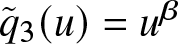 $\tilde{q}_3(u)=u^\beta$ for all
  $u\in[0,1]$ and
  $0\le\beta \lt 1/2$. Therefore Eq. (5.8) becomes
 \begin{equation}
d(u)=\frac{u^{1/3}-u}{u^\beta-u^{1/2}},\qquad u\in[0,1].
\end{equation}
\begin{equation}
d(u)=\frac{u^{1/3}-u}{u^\beta-u^{1/2}},\qquad u\in[0,1].
\end{equation} In the RHS of Figure 3 we show that the function  $d(u)$ given in Eq. (5.10) is increasing for
  $u\in\mathcal{D}$ with some choices of β.
In the following, we provide another distortion-based result by considering different assumptions. The proof is omitted since it follows along the same lines of the ones above. A similar proposition can be stated for the CDF configuration.
Plots of  $d(u)$, for
  $u\in[0,1]$, given in Eq. (5.9) (left) for
  $\alpha=0.5,0.2,0.1$ (full, dashed and dotted, respectively), and of
  $d(u)$, for
  $u\in[0,1]$, given in Eq. (5.10) (right) for
  $\beta=0.33,0.25,0.2$ (full, dashed and dotted, respectively).

Let X be a random variable having SF  $\overline{F}$. Let
  $\tilde{q}_1$ and
  $\tilde{q}_2$ be distortion functions such that
  $\tilde{q}_1(u)\ge u\ge \tilde{q}_2(u)$ for all
  $u\in[0,1]$. Let Y have distorted SF
  $\overline{F}_1=\tilde{q}_1(\overline{F})$ such that
  $-\infty \lt \mathsf{E}[X] \lt \mathsf{E}[Y] \lt +\infty$ and let
  $\hat{X}$ have distorted SF
  $\overline{F}_2=\tilde{q}_2(\overline{F}_1)$, such that
  $-\infty \lt \mathsf{E}[\hat{X}] \lt \mathsf{E}[Y] \lt +\infty$. If
  $Z\equiv\Psi(X,Y)$ and
  $\hat{Z}\equiv\Psi(\hat{X},Y)$, then
  $Z\le_{lr}\hat{Z}$ iff the function
 \begin{equation*}
r(u){\,:=\,}\frac{\tilde{q}_1(u)-u}{\tilde{q}_1(u)-\tilde{q}_2(\tilde{q}_1(u))}
\end{equation*}
\begin{equation*}
r(u){\,:=\,}\frac{\tilde{q}_1(u)-u}{\tilde{q}_1(u)-\tilde{q}_2(\tilde{q}_1(u))}
\end{equation*} is increasing in  $u\in\mathcal{R}{\,:=\,}\{u\in(0,1): \tilde{q}_1(u) \gt \tilde{q}_2(\tilde{q}_1(u))\}$.
When X and Y have SFs  $\overline{F}$ and
  $\overline{G}$, respectively, then the Receiver Operating Characteristic (ROC) curve between X and Y is defined as
  $ROC_{\overline{G},\overline{F}}(u){\,:=\,}\overline{G}(\overline{F}^{-1}(u))$ for
  $u\in[0,1]$. If X and Y possess absolutely continuous distributions, with an interval support having the same initial point, then the ROC curve is a proper distortion function, as discussed in Capaldo et al. [Reference Capaldo, Di Crescenzo and Pellerey5]. Therefore, analogously to Theorems 5.2 and 5.3, one can characterize the likelihood ratio order between two random variables having PDFs as in Eq. (5.1) by using the ROC curve distortions between the respective baseline ordered random variables.
6. Applications to risk theory
We now apply the equilibrium PDFs studied so far to some risk measures that are useful in insurance and actuarial sciences. Further connections between the PDF in Eq. (5.1) and insurance premium principles have been already explored in Psarrakos [Reference Psarrakos27]. We provide some stochastic comparisons and aging results between risks. Unimodality issues are included as well, with special reference to conditions leading to unimodality with mode equal to the VaR.
We assume that a non-negative random variable X, namely risk, represents the random amount of money paid by an insurance company to indemnify a policyholder, a beneficiary and/or a third-party in execution of an insurance contract (cf. Denuit et al. [Reference Denuit, Dhaene, Goovaerts and Kaas9]).
If X is a risk, with CDF F, then the (right-continuous) VaR corresponding to X is defined as  $\mathsf{VaR}[X;p]{\,:=\,} F^{-1}(p)$, for
  $p\in(0,1)$. Note that
  $X\le_{st} Y$ iff
  $\mathsf{VaR}[X;p]\le\mathsf{VaR}[Y;p]$, for all
  $p\in(0,1)$. Moreover, the Conditional Tail Expectation (CTE) of X is defined as
 \begin{equation*}
\mathsf{CTE}[X;p]{\,:=\,}\mathsf{E}\left[X|X \gt \mathsf{VaR}[X;p]\right],\qquad p\in(0,1)
\end{equation*}
\begin{equation*}
\mathsf{CTE}[X;p]{\,:=\,}\mathsf{E}\left[X|X \gt \mathsf{VaR}[X;p]\right],\qquad p\in(0,1)
\end{equation*} and it represents the conditional expected loss given that the loss exceeds its VaR. Note that  $\mathsf{CTE}[X;0]=\mathsf{E}[X]=\int_{0}^{1}\mathsf{VaR}[X;u]{\rm d}u$.
Remark 6.1. Let X be a risk with CDF F and SF  $\overline{F}$. If
  $X^*$ has distorted CDF
  $F_q=q(F)$ through the following distortion function
 \begin{equation}
q(u){\,:=\,}
\begin{cases}
0,&\quad 0\le u\le p,\\
\displaystyle\frac{u-p}{1-p},&\quad p\le u\le 1,\\
\end{cases}
\end{equation}
\begin{equation}
q(u){\,:=\,}
\begin{cases}
0,&\quad 0\le u\le p,\\
\displaystyle\frac{u-p}{1-p},&\quad p\le u\le 1,\\
\end{cases}
\end{equation} defined for any  $p\in(0,1)$, then
  $X^*=_{st}\left[X|X \gt \mathsf{VaR}[X;p]\right]$ and therefore
  $\mathsf{E}[X^*]=\mathsf{CTE}[X;p]$. Moreover, from Eq. (6.1), since
  $q(u)\le u$ for all
  $u\in(0,1)$, then
  $X\le_{st}X^*$. For any
  $p\in(0,1)$, one also has
  $\mathsf{E}[X] \lt \mathsf{CTE}[X;p]$. Hence, if
  $\mathsf{CTE}[X;p] \lt +\infty$, from Proposition 5.1 the random variable
  $Z\equiv\Psi(X,X^*)$ has PDF given by
 \begin{equation*}
f_{Z}(t)=
\begin{cases}
\displaystyle \frac{F(t)}{\mathsf{CTE}[X;p]-\mathsf{E}[X]},&\qquad t\le\mathsf{VaR}[X;p],\\
\displaystyle\frac{p}{1-p}\frac{\overline{F}(t)}{\mathsf{CTE}[X;p]-\mathsf{E}[X]},&\qquad t\ge\mathsf{VaR}[X;p],\\[2mm]
\end{cases}
\end{equation*}
\begin{equation*}
f_{Z}(t)=
\begin{cases}
\displaystyle \frac{F(t)}{\mathsf{CTE}[X;p]-\mathsf{E}[X]},&\qquad t\le\mathsf{VaR}[X;p],\\
\displaystyle\frac{p}{1-p}\frac{\overline{F}(t)}{\mathsf{CTE}[X;p]-\mathsf{E}[X]},&\qquad t\ge\mathsf{VaR}[X;p],\\[2mm]
\end{cases}
\end{equation*} which is unimodal with mode  $\nu=\mathsf{VaR}[X;p]$.
Another important risk measure is the Tail Value-at-Risk corresponding to X, defined as
 \begin{equation}
\mathsf{TVaR}[X;p]{\,:=\,}\frac1{1-p}\int_{p}^{1}\mathsf{VaR}[X;u]{\rm d}u,\qquad p\in(0,1).
\end{equation}
\begin{equation}
\mathsf{TVaR}[X;p]{\,:=\,}\frac1{1-p}\int_{p}^{1}\mathsf{VaR}[X;u]{\rm d}u,\qquad p\in(0,1).
\end{equation} Note that, if X has an absolutely continuous distribution, then  $\mathsf{CTE}[X;p]=\mathsf{TVaR}[X;p]$, for all
  $p\in(0,1)$. For properties and further relations between these and other risk measures we refer the reader to Section 2 in Denuit et al. [Reference Denuit, Dhaene, Goovaerts and Kaas9].
We recall that the Lorenz curve of X is defined as
 \begin{equation}
\mathsf{L}_X(p){\,:=\,}\frac{\int_{0}^{p}\mathsf{VaR}[X;u]{\rm d}u}{\int_{0}^{1}\mathsf{VaR}[X;u]{\rm d}u}=1-\frac{(1-p)\mathsf{TVaR}[X;p]}{\mathsf{TVaR}[X;0]},\qquad p\in(0,1),
\end{equation}
\begin{equation}
\mathsf{L}_X(p){\,:=\,}\frac{\int_{0}^{p}\mathsf{VaR}[X;u]{\rm d}u}{\int_{0}^{1}\mathsf{VaR}[X;u]{\rm d}u}=1-\frac{(1-p)\mathsf{TVaR}[X;p]}{\mathsf{TVaR}[X;0]},\qquad p\in(0,1),
\end{equation} where the latter equality is due to Eq. (6.2). The Lorenz curve is useful in economics since it provides a graphical representation of income or wealth inequality, see Section 3.4 in Denuit et al. [Reference Denuit, Dhaene, Goovaerts and Kaas9]. Note that  $\mathsf{L}_X$ is a proper distortion function, and thus it is a CDF with support included in
  $[0,1]$.
In the absolutely continuous case, the Lorenz curve of a risk is related to its equilibrium PDF and the equilibrium PDF of the corresponding distorted version through the distortion given in Eq. (6.1), as shown below.
Remark 6.2. Let  $X^*$ have distorted CDF as introduced in Remark 6.1. From Eqs. (1.1) and (6.3), if X has an absolutely continuous distribution, then its Lorenz curve can be expressed as
 \begin{equation*}
\mathsf{L}_X(p)=1-\frac{f^e(\mathsf{VaR}[X;p])}{f^e_*(\mathsf{VaR}[X;p])},\qquad p\in(0,1),
\end{equation*}
\begin{equation*}
\mathsf{L}_X(p)=1-\frac{f^e(\mathsf{VaR}[X;p])}{f^e_*(\mathsf{VaR}[X;p])},\qquad p\in(0,1),
\end{equation*} where  $f^e(t)$, for
  $t\ge0$, is the equilibrium PDF of X, while
  $f^e_*(t)$, for
  $t\ge\mathsf{VaR}[X;p]$ and
  $p\in(0,1)$, is the equilibrium PDF of
  $X^*$ with the distortion defined in Eq. (6.1).
We now provide some results under the following assumptions.
Assumptions 6.1. Let X and Y be risks such that  $X\le_{st}Y$ and
  $\mathsf{E}[X] \lt \mathsf{E}[Y] \lt +\infty$. Let
  $Z\equiv\Psi(X,Y)$. We assume that the CDFs of
  $X^*$ and
  $Y^*$ are obtained by applying the distortion given in Eq. (6.1) to the CDFs of X and Y, respectively. We also assume that
  $\mathsf{CTE}[X;p] \lt \mathsf{CTE}[Y;p] \lt +\infty$, for any
  $p\in(0,1)$.
Note that, under Assumptions 6.1, since  $X^*\le_{st}Y^*$, then
  $Z^*\equiv\Psi(X^*,Y^*)$ has PDF
 \begin{equation}
f_{Z*}(t)=
\begin{cases}
\displaystyle 0,&\qquad t\le\mathsf{VaR}[X;p],\\
\displaystyle\frac{F_X(t)-p}{(1-p)\left\{\mathsf{CTE}[Y;p]-\mathsf{CTE}[X;p]\right\}},&\qquad\mathsf{VaR}[X;p]\le t\le\mathsf{VaR}[Y;p],\\[2mm]
\displaystyle f_Z(t)\frac{\mathsf{E}[Y]-\mathsf{E}[X]}{(1-p)\left\{\mathsf{CTE}[Y;p]-\mathsf{CTE}[X;p]\right\}},&\qquad t\ge\mathsf{VaR}[Y;p]\\
\end{cases}
\end{equation}
\begin{equation}
f_{Z*}(t)=
\begin{cases}
\displaystyle 0,&\qquad t\le\mathsf{VaR}[X;p],\\
\displaystyle\frac{F_X(t)-p}{(1-p)\left\{\mathsf{CTE}[Y;p]-\mathsf{CTE}[X;p]\right\}},&\qquad\mathsf{VaR}[X;p]\le t\le\mathsf{VaR}[Y;p],\\[2mm]
\displaystyle f_Z(t)\frac{\mathsf{E}[Y]-\mathsf{E}[X]}{(1-p)\left\{\mathsf{CTE}[Y;p]-\mathsf{CTE}[X;p]\right\}},&\qquad t\ge\mathsf{VaR}[Y;p]\\
\end{cases}
\end{equation} and it represents the equilibrium PDF of two ordered truncated risks in their respective VaR at the same probability level  $p\in(0,1)$.
We remark that the condition  $\mathsf{CTE}[X;p] \lt \mathsf{CTE}[Y;p] \lt +\infty$, for any
  $p\in(0,1)$, given in Assumptions 6.1, is not a consequence of the conditions
  $X\le_{st}Y$ and
  $\mathsf{E}[X] \lt \mathsf{E}[Y] \lt +\infty$. Indeed, for instance, if X is standard uniformly distributed and Y has CDF
 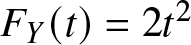 $F_Y(t)=2t^2$ for
  $0\leq t \lt 1/2$ and
  $F_Y(t)=t$ for
  $1/2\leq t\leq 1$, then
  $X\le_{st}Y$ and
  $1/2=\mathsf{E}[X] \lt \mathsf{E}[Y]=13/24$, but
  $\mathsf{CTE}[X;1/2]=\mathsf{CTE}[Y;1/2]=3/4$.
The unimodality of  $Z^*$ is related to that of Z, as shown below.
Proposition 6.1. Under the Assumptions 6.1, for  $p\in(0,1)$, if Z is unimodal with mode
  $\nu\ge\mathsf{VaR}[Y;p]$, then
  $Z^*$ is unimodal with mode ν.
In the following, we obtain sufficient conditions on the risks X, Y and on  $Z\equiv\Psi(X,Y)$ leading to the unimodality of
  $Z^*\equiv\Psi(X^*,Y^*)$ in the VaR of Y.
Proposition 6.2. Under the Assumptions 6.1, for  $p\in(0,1)$, if
  $F_X(t)$ is strictly increasing for
  $t\in\left(\mathsf{VaR}[X;p],\mathsf{VaR}[Y;p]\right)$, and if Z has decreasing HR
  $\lambda_Z(t)$ for
  $t\ge\mathsf{VaR}[Y;p]$, then
  $Z^*$ is unimodal with mode
  $\nu=\mathsf{VaR}[Y;p]$.
Proof. Since  $\lambda_Z(t)$ is decreasing for
  $t\ge\mathsf{VaR}[Y;p]$, then
  $f_Z(t)$ is decreasing for
  $t\ge\mathsf{VaR}[Y;p]$, for
  $p\in(0,1)$. Hence, the result follows from Eq. (6.4).
Corollary 6.1. Under the Assumptions 6.1, for  $p\in(0,1)$, if
  $F_X(t)$ is strictly increasing for
  $t\in(0,+\infty)$ and Z is DFR, then
  $Z^*$ is unimodal with mode
  $\nu=\mathsf{VaR}[Y;p]$.
Hereafter, we show sufficient conditions on the risks X and Y aiming to compare Z and  $Z^*$ in likelihood ratio or reversed hazard rate orders.
Proposition 6.3. Under the Assumptions 6.1, for  $p\in(0,1)$, if
  $F_X(t)/F_Y(t)$ is decreasing for
  $t\in\left(\mathsf{VaR}[X;p],\mathsf{VaR}[Y;p]\right)$, then
  $Z\le_{lr}Z^*$.
Proof. From Eq. (6.4), under the stated hypothesis, the likelihood ratio function
 \begin{equation*}
\frac{f_Z(t)}{f_{Z^*}(t)}=
\begin{cases}
\displaystyle\frac{F_X(t)-F_Y(t)}{F_X(t)-p}\cdot\frac{(1-p)\left\{\mathsf{CTE}[Y;p]-\mathsf{CTE}[X;p]\right\}}{\mathsf{E}[Y]-\mathsf{E}[X]},&\quad\mathsf{VaR}[X;p] \lt t\le\mathsf{VaR}[Y;p],\\
\displaystyle\frac{(1-p)\left\{\mathsf{CTE}[Y;p]-\mathsf{CTE}[X;p]\right\}}{\mathsf{E}[Y]-\mathsf{E}[X]},&\quad t\ge\mathsf{VaR}[Y;p],\\
\end{cases}
\end{equation*}
\begin{equation*}
\frac{f_Z(t)}{f_{Z^*}(t)}=
\begin{cases}
\displaystyle\frac{F_X(t)-F_Y(t)}{F_X(t)-p}\cdot\frac{(1-p)\left\{\mathsf{CTE}[Y;p]-\mathsf{CTE}[X;p]\right\}}{\mathsf{E}[Y]-\mathsf{E}[X]},&\quad\mathsf{VaR}[X;p] \lt t\le\mathsf{VaR}[Y;p],\\
\displaystyle\frac{(1-p)\left\{\mathsf{CTE}[Y;p]-\mathsf{CTE}[X;p]\right\}}{\mathsf{E}[Y]-\mathsf{E}[X]},&\quad t\ge\mathsf{VaR}[Y;p],\\
\end{cases}
\end{equation*} is decreasing in t, i.e.,  $Z\le_{lr}Z^*$.
Corollary 6.2. Under the Assumptions 6.1, if  $X\le_{rhr}Y$, then
  $Z\le_{lr}Z^*$. Therefore:
• If
$X\le_{rhr}Y$, then
$Z\le_{rhr}Z^*$.• If X and Y have absolutely continuous distributions and
$X\le_{lr}Y$, then
$Z\le_{lr}Z^*$.


The ILR property of  $Z^*$ can be obtained under suitable aging assumptions on the risk X and the corresponding Z, as illustrated below.
Proposition 6.4. Under the Assumptions 6.1, let X have an absolutely continuous distribution with decreasing HR  $\lambda_X(t)$ for
  $t\in\left(\mathsf{VaR}[X;p],\mathsf{VaR}[Y;p]\right)$, for
  $p\in(0,1)$. If Z has increasing Glaser’s function
  $\eta_Z(t)$ for
  $t\ge\mathsf{VaR}[Y;p]$, then
  $Z^*$ is ILR.
Proof. For  $p\in(0,1)$, the Glaser’s function of
  $Z^*$ is
 \begin{equation*}
\eta_{Z^*}(t)=
\begin{cases}
\displaystyle h(t){\,:=\,}\frac{f_X(t)}{p-F_X(t)},&\qquad\mathsf{VaR}[X;p] \lt t\le\mathsf{VaR}[Y;p],\\
\displaystyle\eta_Z(t),&\qquad t\ge\mathsf{VaR}[Y;p].\\
\end{cases}
\end{equation*}
\begin{equation*}
\eta_{Z^*}(t)=
\begin{cases}
\displaystyle h(t){\,:=\,}\frac{f_X(t)}{p-F_X(t)},&\qquad\mathsf{VaR}[X;p] \lt t\le\mathsf{VaR}[Y;p],\\
\displaystyle\eta_Z(t),&\qquad t\ge\mathsf{VaR}[Y;p].\\
\end{cases}
\end{equation*} Under the stated hypothesis on  $\lambda_X(t)$, one has
  $f_X(t)$ decreasing for
  $t\in\left(\mathsf{VaR}[X;p],\mathsf{VaR}[Y;p]\right)$. Therefore
 \begin{equation*}
h'(t)=\frac{f'_X(t)(p-F_X(t))+f^2_X(t)}{(p-F_X(t))^2}\ge 0,\qquad\mathsf{VaR}[X;p] \lt t\le\mathsf{VaR}[Y;p]
\end{equation*}
\begin{equation*}
h'(t)=\frac{f'_X(t)(p-F_X(t))+f^2_X(t)}{(p-F_X(t))^2}\ge 0,\qquad\mathsf{VaR}[X;p] \lt t\le\mathsf{VaR}[Y;p]
\end{equation*} and the proof is completed since  $\eta_Z(t)$ is increasing for
  $t\ge\mathsf{VaR}[Y;p]$.
Corollary 6.3. Under the Assumptions 6.1, if X is DFR and Z is ILR, then  $Z^*$ is ILR.
We conclude this section with the following ordering result. Under suitable assumptions between three different risks, the corresponding PDFs obtained from Eq. (6.4) are likelihood ratio ordered.
Proposition 6.5. Let X, Y1 and Y2 be risks such that  $X\le_{st}Y_1\le_{st}Y_2$ and
  $\mathsf{E}[X] \lt \mathsf{E}[Y_1] \lt \mathsf{E}[Y_2] \lt +\infty$. Let
  $X^*$,
  $Y^*_1$ and
  $Y^*_2$ have distorted CDFs from the ones of X, Y1 and Y2 through the distortion function given in Eq. (6.1), respectively, such that
  $\mathsf{E}[X^*] \lt \mathsf{E}[Y^*_1] \lt \mathsf{E}[Y^*_2] \lt +\infty$. Let
  $Z_1\equiv\Psi(X,Y_1)$,
  $Z_2\equiv\Psi(X,Y_2)$,
  $Z_1^*\equiv\Psi(X^*,Y_1^*)$ and
  $Z_2^*\equiv\Psi(X^*,Y_2^*)$. If
  $X\le_{rhr}Y_1$ and
  $Z_1\le_{lr}Z_2$, then
  $Z_1^*\le_{lr}Z_2^*$.
Proof. Under the stated assumptions, it is easy to see that the likelihood ratio function
 \begin{equation*}
\frac{f_{Z_1^*}(t)}{f_{Z_2^*}(t)}=
\begin{cases}
\displaystyle\frac{\mathsf{CTE}[Y_2;p]-\mathsf{CTE}[X;p]}{\mathsf{CTE}[Y_1;p]-\mathsf{CTE}[X;p]},&\qquad\mathsf{VaR}[X;p]\le t\le\mathsf{VaR}[Y_1;p],\\
\displaystyle\frac{F_X(t)-F_{Y_1}(t)}{F_X(t)-p}\cdot\frac{\mathsf{CTE}[Y_2;p]-\mathsf{CTE}[X;p]}{\mathsf{CTE}[Y_1;p]-\mathsf{CTE}[X;p]},&\qquad\mathsf{VaR}[Y_1;p]\le t\le\mathsf{VaR}[Y_2;p],\\
\displaystyle\frac{f_{Z_1}(t)}{f_{Z_2}(t)}\cdot\frac{\mathsf{E}[Y_1]-\mathsf{E}[X]}{\mathsf{E}[Y_2]-\mathsf{E}[X]}\cdot\frac{\mathsf{CTE}[Y_2;p]-\mathsf{CTE}[X;p]}{\mathsf{CTE}[Y_1;p]-\mathsf{CTE}[X;p]},&\qquad t\ge\mathsf{VaR}[Y_2;p],\\
\end{cases}
\end{equation*}
\begin{equation*}
\frac{f_{Z_1^*}(t)}{f_{Z_2^*}(t)}=
\begin{cases}
\displaystyle\frac{\mathsf{CTE}[Y_2;p]-\mathsf{CTE}[X;p]}{\mathsf{CTE}[Y_1;p]-\mathsf{CTE}[X;p]},&\qquad\mathsf{VaR}[X;p]\le t\le\mathsf{VaR}[Y_1;p],\\
\displaystyle\frac{F_X(t)-F_{Y_1}(t)}{F_X(t)-p}\cdot\frac{\mathsf{CTE}[Y_2;p]-\mathsf{CTE}[X;p]}{\mathsf{CTE}[Y_1;p]-\mathsf{CTE}[X;p]},&\qquad\mathsf{VaR}[Y_1;p]\le t\le\mathsf{VaR}[Y_2;p],\\
\displaystyle\frac{f_{Z_1}(t)}{f_{Z_2}(t)}\cdot\frac{\mathsf{E}[Y_1]-\mathsf{E}[X]}{\mathsf{E}[Y_2]-\mathsf{E}[X]}\cdot\frac{\mathsf{CTE}[Y_2;p]-\mathsf{CTE}[X;p]}{\mathsf{CTE}[Y_1;p]-\mathsf{CTE}[X;p]},&\qquad t\ge\mathsf{VaR}[Y_2;p],\\
\end{cases}
\end{equation*} is decreasing in t, i.e.,  $Z_1^*\le_{lr}Z_2^*$.
7. Concluding remarks
In this paper, the (unimodal) equilibrium distribution of a random variable having general support is defined and studied by extending results that have been exploited in the past for non-negative random variables. Various stochastic comparisons between baseline distributions are maintained by the corresponding generalized equilibrium distributions. Conditions for the preservation of aging classes are also investigated. A probabilistic analog of Taylor’s theorem is expanded to the case involving the new equilibrium PDF. Results regarding mean-median-mode relations are illustrated as well. The probabilistic analog of the mean value theorem is stated in the case of the extended equilibrium distribution of two ordered random variables. Unimodality conditions and stochastic comparisons related to such extended equilibrium PDF are exhibited. We show that the mentioned equilibrium PDFs are connected through suitable mixture properties (see Eq. (5.2)).
In insurance and actuarial sciences unimodality and stochastic orderings issues are relevant. We apply these equilibrium PDFs to some well-known risk measures. In particular, the Lorenz curve is related with the equilibrium PDF of a given risk and its truncated version in the corresponding VaR. The unimodality of the equilibrium PDF of two ordered truncated risks in the corresponding VaR is related with the unimodality of the equilibrium PDF of the ordered baseline risks. We have shown conditions for which the mode is equal to the VaR of the risks that is greater in the usual stochastic sense.
Future developments could be oriented to define multivariate versions of the proposed generalized equilibrium distributions, along with the different lines described for non-negative random variables in Gupta and Sankaran [Reference Gupta and Sankaran15], Navarro et al. [Reference Navarro, Ruiz and Del Aguila24] and Navarro and Sarabia [Reference Navarro and Sarabia26]. Inference procedures should be proposed and studied in order to manage economics data by using equilibrium distributions.
Acknowledgements
M.C. and A.D.C. are members of the Gruppo Nazionale Calcolo Scientifico-Istituto Nazionale di Alta Matematica (GNCS-INdAM). This work is partially funded by the “European Union—Next Generation EU” through MUR-PRIN 2022, project 2022XZSAFN “Anomalous Phenomena on Regular and Irregular Domains: Approximating Complexity for the Applied Sciences”, and MUR-PRIN 2022 PNRR, project P2022XSF5H “Stochastic Models in Biomathematics and Applications”. J.N. thanks the support of Ministerio de Ciencia e Innovación of Spain in the grant PID2022-137396NB-I00 funded by MCIN/AEI/10.13039/501100011033 and “ERDF A way of making Europe”.
Declaration of interests
The authors have nothing to declare.
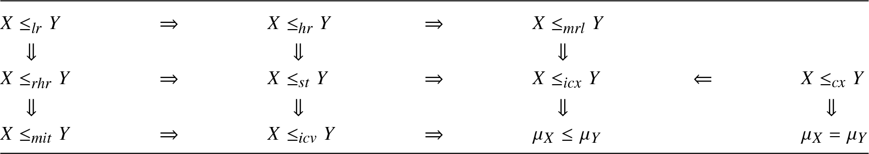
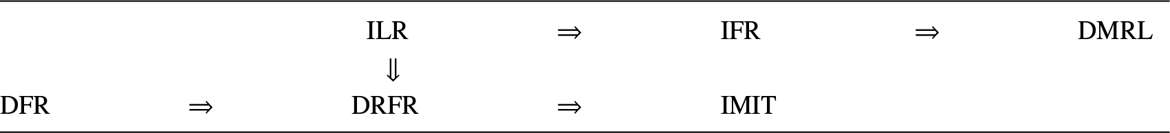
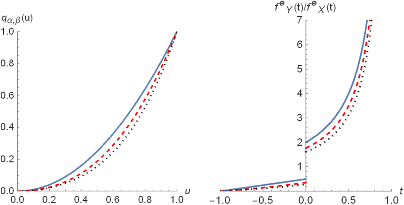

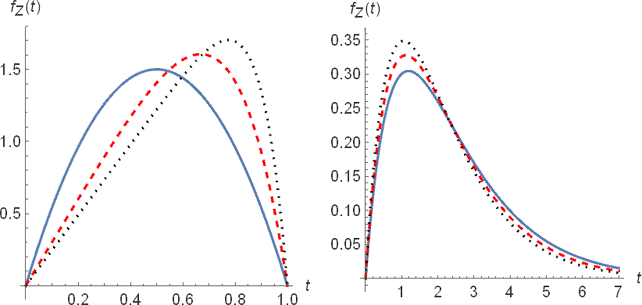


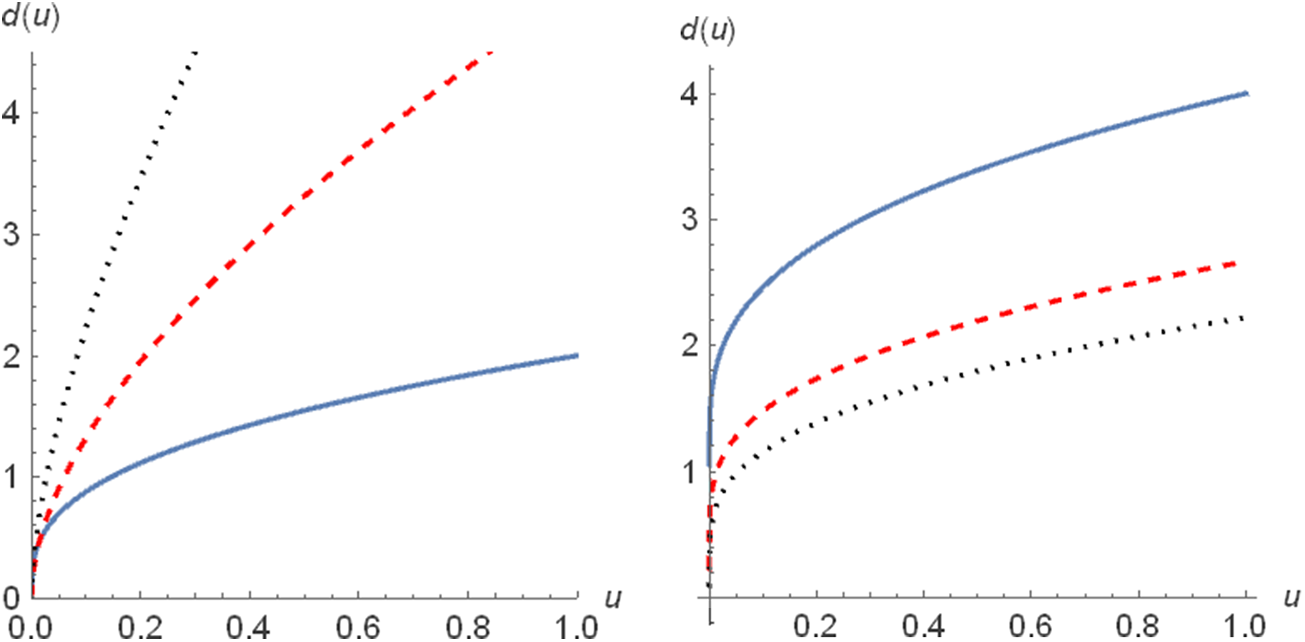


 Open access