


1. Introduction
The concept of entropy was first introduced and thoroughly explored by Shannon [Reference Shannon19], an electrical engineer at Bell Telephone Laboratories, in his research on communication networks. Around the same time, Wiener [Reference Wiener22] independently investigated the concept in his work on Cybernetics, albeit with a different motivation. Let  $X$ be a non-negative rv with an absolutely continuous cumulative distribution function (cdf) $F(x) = P[X \leq x]$ and with probability density function (pdf) $f(x)$. Then the Shannon entropy associated with $X$ is defined as
 \begin{equation}
H(X) = - \int\limits_0^{+\infty} {f(x)\log f(x)\ dx}.
\end{equation}
\begin{equation}
H(X) = - \int\limits_0^{+\infty} {f(x)\log f(x)\ dx}.
\end{equation}Starting from the pioneering work of Shannon [Reference Shannon19], different researchers have shown applications of entropy in different fields. Apart from thermodynamics and information theory, application of Shannon entropy varies over diverse fields such as statistics, economics, finance, psychology, wavelet analysis, image recognition, computer science, fuzzy sets and so on. In spite of its well known applications, it is necessary to modify this measure under different scenarios, specifically the concept of residual entropy proposed by Ebrahimi [Reference Ebrahimi7] substantiate this claim.
If the system has already survived for some units of time, Shannon entropy will not be applicable in such cases which led to the development of residual entropy. Residual entropy is the Shannon entropy associated with the rv  $[X-t|X \gt t]$, $t\geq 0$, and is defined as (see, Ebrahimi [Reference Ebrahimi7])
 \begin{equation}
\begin{aligned}
H(f;t) & = - \int\limits_t^{+\infty} {\frac{{f(x)}}{{\overline F (t)}}\log \left(\frac{{f(x)}}{{\overline F (t)}}\right)dx},
\end{aligned}
\end{equation}
\begin{equation}
\begin{aligned}
H(f;t) & = - \int\limits_t^{+\infty} {\frac{{f(x)}}{{\overline F (t)}}\log \left(\frac{{f(x)}}{{\overline F (t)}}\right)dx},
\end{aligned}
\end{equation} where  $\overline F(t)$ denotes the survival function. Given that an item has survived up to time $t$,
$t$,  $H(f;t)$ measures the uncertainty about its remaining life.
Ebrahimi [Reference Ebrahimi7] used this concept to define new ageing classes such as decreasing (increasing) uncertainty of residual life (DURL (IURL)). Belzunce et al. [Reference Belzunce, Guillamón, Navarro and Ruiz3] proposed kernel-type estimation of the residual entropy function in the case of independent complete data sets. Belzunce et al. [Reference Belzunce, Navarro, Ruiz and del Aguila4] showed that for a rv  $X$ with an increasing residual entropy $H(f;t)$, the function $H(f;t)$ uniquely determines the cdf. Rajesh et al. [Reference Rajesh, Abdul-Sathar, Maya and Nair15] thoroughly elucidated the necessity of developing inferential aspects under dependent sample and proposed non-parametric kernel type estimators for the residual entropy function based on $\alpha$-mixing dependent sample.
Di Crescenzo and Longobardi [Reference Di Crescenzo and Longobardi6] discussed the necessity of developing the uncertainty measure based on the reversed residual life (past lifetime) and they developed the concept of past entropy. If  $X$ denotes the lifetime of a component, a system or a living organism, then the past entropy of $X$ at time $t$ is defined as
 \begin{equation}
\begin{aligned}
\overline H(f;t) & = - \int\limits_0^ t {\frac{{f(x)}}{{F (t)}}\log \frac{{f(x)}}{{F (t)}}\ dx}.
\end{aligned}
\end{equation}
\begin{equation}
\begin{aligned}
\overline H(f;t) & = - \int\limits_0^ t {\frac{{f(x)}}{{F (t)}}\log \frac{{f(x)}}{{F (t)}}\ dx}.
\end{aligned}
\end{equation} This measure has become significant in forensic science, particularly in determining the exact time of failure (or death, in the case of humans) when a unit is found in a failed state at some time  $t$. It also has applications in actuarial science, as discussed by [Reference Sachlas and Papaioannou18]. Maya [Reference Maya12] introduced non-parametric estimators for this measure, applicable to both complete and censored $\alpha$-mixing dependent samples.
Numerous researchers have explored various definitions of entropy and their associated properties. Balakrishnan et al. [Reference Balakrishnan, Buono and Longobardi2] established relationships between certain cumulative entropies and the moments of order statistics. Furthermore, a general formulation of entropy was presented in Balakrishnan et al. [Reference Balakrishnan, Buono and Longobardi1]. Building on the successful applications of the past entropy function, Gupta and Nanda [Reference Gupta and Nanda9] extended (1.3) to define the past entropy function of order  $\beta$. Now the past entropy function of order $\beta$ is defined as
 \begin{equation}
\overline H^\beta (f;t) = \frac{1}{(1-\beta )}\left\{\log \int\limits
_0^t \left(\frac{f (x)}{F (t)}\right)^\beta
dx\right\},\ \text{for} \ \beta \neq 1, \beta \gt 0.
\end{equation}
\begin{equation}
\overline H^\beta (f;t) = \frac{1}{(1-\beta )}\left\{\log \int\limits
_0^t \left(\frac{f (x)}{F (t)}\right)^\beta
dx\right\},\ \text{for} \ \beta \neq 1, \beta \gt 0.
\end{equation}Later on Nanda and Paul [Reference Nanda and Paul13] elucidated certain ordering and ageing properties and some characterization results based on this generalized past entropy measure. As stated by Ebrahimi [Reference Ebrahimi7], systems or components with high uncertainty tend to exhibit lower reliability. Building on this concept, these measures can be effectively used to choose the most reliable system among competing models.
However, in terms of inferential aspects, no studies appear to have been conducted in the existing literature. This gap motivates the authors to explore the development of a non-parametric estimator for the generalized past entropy function using kernel-based estimation. The study focuses on cases where the observations exhibit dependence. More specifically, the proposed estimator is based on an  $\alpha$-mixing dependent sample (see Rosenblatt [Reference Rosenblatt17]), and its definition is provided below.
Definition 1.1. Let  $\{X_i;i\geq 1\}$ denote a sequence of rvs. Given a positive integer $n$, set
 \begin{equation}
\alpha (n) = \sup\limits_ {k \geq 1} \{|P(A \cap B )-P(A)P(B)|;
A\epsilon \mathfrak{F}_1^k, B \epsilon \mathfrak{F}_{k+n}^{+\infty}\},
\end{equation}
\begin{equation}
\alpha (n) = \sup\limits_ {k \geq 1} \{|P(A \cap B )-P(A)P(B)|;
A\epsilon \mathfrak{F}_1^k, B \epsilon \mathfrak{F}_{k+n}^{+\infty}\},
\end{equation} where  $\mathfrak{F}_i^k$ denote the $\sigma$- field of events generated by $\{X_j; i \leq j \leq k\}$. The sequence is said to be $\alpha$-mixing (strong mixing) if the mixing coefficient $\alpha(n)\to 0$ as $n \to +\infty$.
Among various mixing conditions,  $\alpha$-mixing is reasonably weak and has many practical applications. In the same way, Irshad et al. [Reference Irshad, Maya, Buono and Longobardi10] have proposed non-parametric kernel type estimators for two versions of cumulative residual Tsallis entropies.
The rest of the article is organized as follows. In Section 2, we propose a non-parametric kernel type estimator of  $\overline H^{\beta}(f;t)$ given in (1.4) by $\alpha$-mixing dependent sample. Asymptotic properties of the proposed estimator are discussed in Section 3. The performance of the estimator is validated using simulation study in Section 4. In Section 5, a real data set is used to illustrate the performance of the proposed estimator and then the asymptotic normality is analyzed by the use of histograms. Finally, the article is concluded in Section 6.
2. Non-parametric estimation of generalized past entropy function
In this section, we propose a non-parametric kernel type estimator for the generalized past entropy function.
Let  $\{X_i; 1\leq i\leq n\}$ be a sequence of identically distributed rvs. Note that $X{_i}'s$ need not be mutually independent, that is, the observations are supposed to be $\alpha$-mixing. Rosenblatt [Reference Rosenblatt16] and Parzen [Reference Parzen14] proposed a non-parametric kernel type estimator of $f (x)$ that is given by
 \begin{equation}
f_n (x) = \frac{1}{n b_n}\sum\limits_{j = 1}^n {K\left( {\frac{{x -
X_j }}{{b_n }}} \right)},
\end{equation}
\begin{equation}
f_n (x) = \frac{1}{n b_n}\sum\limits_{j = 1}^n {K\left( {\frac{{x -
X_j }}{{b_n }}} \right)},
\end{equation} where  $K(x)$ is a kernel of order $s$ satisfying the conditions:
a. $K(x) \geq 0$ for all
$x$,
$K(x) \geq 0$ for all
$x$,b.
$\int\limits_{- +\infty }^{+\infty} K(x)dx = 1$,c.
$K(\cdot)$ is symmetric about zero and satisfies the Lipschitz condition, that is, there exists a constant
$M$ such that
$|K(x)-K(y)| \leq M |x-y|$,d.
$K_n (x) = \frac{1}{b_n} {K\left( {\frac{{x }}{{b_n }}} \right)}$, where
$\{b_n\}$ is a bandwidth sequence of positive numbers such that
$b_n \rightarrow 0$ and
$nb_n \rightarrow +\infty$ as
$n \rightarrow +\infty$.


The expressions for the bias and variance of  $f_n (x)$ under $\alpha$-mixing dependence sample are respectively given by
 \begin{equation}
Bias\mathop {}\limits^{} (f_n (x)) \backsimeq \frac{{b_n ^s
\Delta_s}}{{s!}}f^{(s)} (x)
\end{equation}
\begin{equation}
Bias\mathop {}\limits^{} (f_n (x)) \backsimeq \frac{{b_n ^s
\Delta_s}}{{s!}}f^{(s)} (x)
\end{equation}and
 \begin{equation}
Var\mathop {}\limits^{} (f_n (x)) \backsimeq \frac{{
f(x)}}{{nb{}_n}}\Delta_K,
\end{equation}
\begin{equation}
Var\mathop {}\limits^{} (f_n (x)) \backsimeq \frac{{
f(x)}}{{nb{}_n}}\Delta_K,
\end{equation} where  $\Delta_s = \int\limits_{- +\infty }^{+\infty} {u^s K(u)\ du} $, $\Delta_K = \int\limits_{- +\infty }^{+\infty} {K^2 (u)\ du}$ and $f^{(s)}(\cdot)$ denotes the $s$-th derivative of $f$.
$f$.
Based on (2.1), we propose a non-parametric kernel type estimator for  $\overline H^{\beta} (f;t)$ that is defined as
 \begin{equation}
\overline H_n^\beta (f;t) = \frac{1}{(1-\beta)}\left\{\log \int\limits_0 ^
t f_n^\beta (x)\ dx - \beta \log F_n (t) \right\},
\end{equation}
\begin{equation}
\overline H_n^\beta (f;t) = \frac{1}{(1-\beta)}\left\{\log \int\limits_0 ^
t f_n^\beta (x)\ dx - \beta \log F_n (t) \right\},
\end{equation} where  $f_n (x)$ is a non-parametric estimator of $f (x)$ and is given in (2.1) and $ F_n (t)= \int\limits_0^t f_n (x) dx $ is a non-parametric estimator of cdf $ F (t)$. The bias and variance of $ F_n (t)$ are respectively given by (see, Maya [Reference Maya12])
 \begin{equation}
Bias\mathop {}\limits^{}(F_n (t)) \backsimeq \frac{b_n^{s}\Delta_{s}
}{s!}\int\limits_0^t f^{(s)}(x)\ dx
\end{equation}
\begin{equation}
Bias\mathop {}\limits^{}(F_n (t)) \backsimeq \frac{b_n^{s}\Delta_{s}
}{s!}\int\limits_0^t f^{(s)}(x)\ dx
\end{equation}and
 \begin{equation}
Var\mathop {}\limits^{} (F_n (t)) \backsimeq \frac{1}{nb_n}
\Delta_K F(t).
\end{equation}
\begin{equation}
Var\mathop {}\limits^{} (F_n (t)) \backsimeq \frac{1}{nb_n}
\Delta_K F(t).
\end{equation}3. Asymptotic properties of generalized past entropy function
In this section, some asymptotic properties of generalized past entropy function are established.
For computational simplicity, define the following
 \begin{equation}
a_n (t) = \log\int\limits_0^t {f_n^{\beta} (x)\ dx},a(t) =
\log\int\limits_0^t {f^{\beta} (x)\ dx},
\end{equation}
\begin{equation}
a_n (t) = \log\int\limits_0^t {f_n^{\beta} (x)\ dx},a(t) =
\log\int\limits_0^t {f^{\beta} (x)\ dx},
\end{equation}and
 \begin{equation}
m_n (t)=\log F_n (t)\ \text{and} \ m(t)=\log F(t).
\end{equation}
\begin{equation}
m_n (t)=\log F_n (t)\ \text{and} \ m(t)=\log F(t).
\end{equation}Therefore,
 \begin{equation}
\overline H^\beta (f;t) = \frac{1}{(1-\beta)}\left[ a(t)- \beta\ m
(t) \right]
\end{equation}
\begin{equation}
\overline H^\beta (f;t) = \frac{1}{(1-\beta)}\left[ a(t)- \beta\ m
(t) \right]
\end{equation}and
 \begin{equation}
\overline H_n^\beta (f;t) = \frac{1}{(1-\beta)}\left[ a_n (t)- \beta\ m_n
(t) \right].
\end{equation}
\begin{equation}
\overline H_n^\beta (f;t) = \frac{1}{(1-\beta)}\left[ a_n (t)- \beta\ m_n
(t) \right].
\end{equation} In the following theorems, the weak and strong consistency properties of  $\overline H_n^\beta (f;t)$ are proved.
Theorem 3.1. Suppose  $\overline H_n^\beta (f;t)$ is a non-parametric estimator of $\overline H^\beta (f;t)$ defined in (2.4) satisfying the assumptions given in Section 2. Then $\overline H_n^\beta (f;t) $ is a consistent estimator of $\overline H^\beta (f;t) $.
Proof. By using Taylor’s series expansion, we have
 \begin{equation*}
\log\int\limits_0^t {f_n^{\beta} (x)\ dx}\backsimeq
\log\int\limits_0^t {f^{\beta} (x)\ dx}+(f_n(t)-f(t))\frac{\int\limits_0^t\beta f^{\beta-1}(x)dx }{\int\limits_0^t f^\beta(x)dx}.
\end{equation*}
\begin{equation*}
\log\int\limits_0^t {f_n^{\beta} (x)\ dx}\backsimeq
\log\int\limits_0^t {f^{\beta} (x)\ dx}+(f_n(t)-f(t))\frac{\int\limits_0^t\beta f^{\beta-1}(x)dx }{\int\limits_0^t f^\beta(x)dx}.
\end{equation*}Using (3.1), we get
 \begin{equation}
a_n(t) \backsimeq a(t)+(f_n(t)-f(t))u(t),
\end{equation}
\begin{equation}
a_n(t) \backsimeq a(t)+(f_n(t)-f(t))u(t),
\end{equation}where
 \begin{equation*}u(t)=\frac{\int\limits_0^t\beta f^{\beta-1}(x)dx }{\int\limits_0^t f^\beta(x)dx}.\end{equation*}
Also,
 \begin{equation*}
\log F_n (t) \backsimeq\log F(t)+\frac{(F_n(t)-F(t))}{F(t)}.
\end{equation*}
\begin{equation*}
\log F_n (t) \backsimeq\log F(t)+\frac{(F_n(t)-F(t))}{F(t)}.
\end{equation*}From (3.2), we write
 \begin{equation}
m_n(t) \backsimeq m(t)+\frac{(F_n(t)-F(t))}{F(t)},
\end{equation}
\begin{equation}
m_n(t) \backsimeq m(t)+\frac{(F_n(t)-F(t))}{F(t)},
\end{equation} Using (3.5) and (3.6), the bias and variance of  $a_n(t)$ and $m_n(t)$ are given by
 \begin{equation}
Bias\mathop {}\limits^{}(a_n (t)) \backsimeq \frac{b_n^{s}}{s!}\Delta_{s}
f^{(s)}(t)u(t),
\end{equation}
\begin{equation}
Bias\mathop {}\limits^{}(a_n (t)) \backsimeq \frac{b_n^{s}}{s!}\Delta_{s}
f^{(s)}(t)u(t),
\end{equation} \begin{equation}
Var\mathop {}\limits^{} (a_n (t)) \backsimeq \frac{1}{nb_n}
\Delta_Kf(t)u^2(t),
\end{equation}
\begin{equation}
Var\mathop {}\limits^{} (a_n (t)) \backsimeq \frac{1}{nb_n}
\Delta_Kf(t)u^2(t),
\end{equation} \begin{equation}
Bias\mathop {}\limits^{}(m_n (t)) \backsimeq \frac{b_n^{s}\Delta_{s}
}{s!F(t)}\int\limits_0^t f^{(s)}(x)\ dx,
\end{equation}
\begin{equation}
Bias\mathop {}\limits^{}(m_n (t)) \backsimeq \frac{b_n^{s}\Delta_{s}
}{s!F(t)}\int\limits_0^t f^{(s)}(x)\ dx,
\end{equation}and
 \begin{equation}
Var\mathop {}\limits^{} (m_n (t)) \backsimeq \frac{1}{nb_n}
\frac{\Delta_K} {F(t)}.
\end{equation}
\begin{equation}
Var\mathop {}\limits^{} (m_n (t)) \backsimeq \frac{1}{nb_n}
\frac{\Delta_K} {F(t)}.
\end{equation} From (3.7) and (3.8), as  $ n \to +\infty$
 \begin{equation*}
\text{MSE} \left( {a_n (t)} \right) \to 0.
\end{equation*}
\begin{equation*}
\text{MSE} \left( {a_n (t)} \right) \to 0.
\end{equation*} Therefore, the estimator  $a_n(t)$ is consistent (in the probability sense), i.e.,
 \begin{equation*}
{a_n (t)}\mathop \to \limits ^ p a(t).
\end{equation*}
\begin{equation*}
{a_n (t)}\mathop \to \limits ^ p a(t).
\end{equation*} From (3.9) and (3.10), as  $ n \to +\infty$
 \begin{equation*}
\text{MSE} \left( {m_n (t)} \right) \to 0.
\end{equation*}
\begin{equation*}
\text{MSE} \left( {m_n (t)} \right) \to 0.
\end{equation*} Therefore, the estimator  $m_n(t)$ is consistent (in the probability sense), i.e.,
 \begin{equation*}
{m_n (t)}\mathop \to \limits ^ p m(t).
\end{equation*}
\begin{equation*}
{m_n (t)}\mathop \to \limits ^ p m(t).
\end{equation*}Therefore
 \begin{equation*}
\overline H_n^\beta (f;t) =\frac{1}{(1-\beta)}\left[ a_n (t)-
\beta\ m_n (t) \right] \mathop \to \limits^p
\frac{1}{(1-\beta)}\left[a(t) -\beta\ m(t)\right]= \overline H^\beta (f;t) .
\end{equation*}
\begin{equation*}
\overline H_n^\beta (f;t) =\frac{1}{(1-\beta)}\left[ a_n (t)-
\beta\ m_n (t) \right] \mathop \to \limits^p
\frac{1}{(1-\beta)}\left[a(t) -\beta\ m(t)\right]= \overline H^\beta (f;t) .
\end{equation*} That is,  $\overline H_n^\beta (f;t)$ is a consistent (in the probability sense) estimator of $\overline H^\beta (f;t)$.
Theorem 3.2. Let  $\overline H_n^\beta (f;t)$ be a non-parametric estimator of $\overline H^\beta (f;t)$ defined in (2.4) satisfying the assumptions given in Section 2. Suppose the kernel $K(\cdot)$ satisfies the requirements:
a.
$K(u)\to 0$ as
$|u|\to +\infty$,b.
$\int\limits_{- +\infty }^{+\infty} |K^{'}(u)| du \lt +\infty$,c.
$\int\limits_{- +\infty }^{+\infty} |u| K(u)\ du \lt +\infty$.
Let  $\overline t=\sup \{t \in \mathbb R; F(t) \lt 1\}$ and $J$ be any compact subset of $(0,\ \overline t)$. Then
 \begin{equation*}
\lim \limits _{n \to +\infty} \sup \limits_ {t
\epsilon J} \left|\overline H_n^\beta (f;t)-\overline H^\beta (f;t)\right|=
0 \ a.s.
\end{equation*}
\begin{equation*}
\lim \limits _{n \to +\infty} \sup \limits_ {t
\epsilon J} \left|\overline H_n^\beta (f;t)-\overline H^\beta (f;t)\right|=
0 \ a.s.
\end{equation*}Proof. By direct calculations, we get
 \begin{equation*}
\begin{aligned}
\overline H_n^\beta (f;t)-\overline H^\beta (f;t)&= \frac{1}{(1-\beta)}\left(a_n
(t)-a(t)\right)-\frac{\beta}{(1-\beta)}\left(m_n (t)-m(t)\right).\\
\end{aligned}
\end{equation*}
\begin{equation*}
\begin{aligned}
\overline H_n^\beta (f;t)-\overline H^\beta (f;t)&= \frac{1}{(1-\beta)}\left(a_n
(t)-a(t)\right)-\frac{\beta}{(1-\beta)}\left(m_n (t)-m(t)\right).\\
\end{aligned}
\end{equation*} \begin{equation*}\nonumber
\begin{aligned}
|\overline H_n^\beta (f;t)-\overline H^\beta (f;t)|
& \backsimeq \frac{u(t)}{(1-\beta)}\left|f_n
(t)-f(t)\right|+\frac{\beta}{(1-\beta)}\left(\frac{| F_n
(t)- F(t)|}{1- F(t)}\right).
\end{aligned}
\end{equation*}
\begin{equation*}\nonumber
\begin{aligned}
|\overline H_n^\beta (f;t)-\overline H^\beta (f;t)|
& \backsimeq \frac{u(t)}{(1-\beta)}\left|f_n
(t)-f(t)\right|+\frac{\beta}{(1-\beta)}\left(\frac{| F_n
(t)- F(t)|}{1- F(t)}\right).
\end{aligned}
\end{equation*} By using Theorem 3.3 and Theorem 4.1 of Cai and Roussas [Reference Cai and Roussas5], the result is immediate. Thus, we conclude that  $\overline H_n^\beta (f;t)$ is a strong consistent estimator of $\overline H^\beta (f;t)$.
In order to prove that  $\overline H_n^\beta (f;t)$ is an integratedly uniformly consistent in quadratic mean estimator of $\overline H^\beta (f;t)$, we consider the following definition from Wegman [Reference Wegman21].
Definition 3.1. The density estimator  $f_n(x)$ is said to be integratedly uniformly consistent in quadratic mean if the mean integrated squared error (MISE) approaches zero, i.e.,
 \begin{equation*}
\lim_{n \to +\infty} \mathbb{E} \left[ \int (f_n(x) -f(x))^2 \,dx \right] = 0
\end{equation*}
\begin{equation*}
\lim_{n \to +\infty} \mathbb{E} \left[ \int (f_n(x) -f(x))^2 \,dx \right] = 0
\end{equation*} In the following theorem, we prove that  $\overline H_n^\beta (f;t)$ is integratedly uniformly consistent in quadratic mean estimator of $\overline H^\beta (f;t)$.
Theorem 3.3. Suppose  $\overline H_n^\beta (f;t)$ is a kernel estimator of $\overline H^\beta (f;t)$ as defined in (2.4). Then, $\overline H_n^\beta (f;t)$ is integratedly uniformly consistent in quadratic mean estimator of $\overline H^\beta (f;t)$.
Proof. MISE of  $\overline H_n^\beta (f;t)$ is given by
 \begin{equation}
\begin{aligned}
{\rm MISE}(\overline H_n^\beta (f;t))&= {\rm E} \int\limits_{0}^{+\infty} \left[\overline H_n^\beta (f;t)-\overline H^\beta (f;t)\right]^2 dt\\
& =\int\limits_{0}^{+\infty} \left[[{\rm Bias}(\overline H_n^\beta (f;t))]^2+{\rm Var}(\overline H_n^\beta (f;t)) \right]dt\\
&= \int\limits_0^{+\infty}\left( \frac{b^{s}_n \Delta_s }{(1-\beta)s!} \left(f^{(s)}(t) u(t)-\frac{\beta}{F(t)} \int\limits_{0}^ {t} f^{(s)}(x) dx \right) \right)^2 dt\\
& +\int\limits_0^{+\infty} \left(\frac{\Delta_K}{nb_n(1-\beta)^{2}} \left(f(t) u^{2}(t)+\frac{\beta^{2}}{F(t)} \right)\right) dt.\\
\end{aligned}
\end{equation}
\begin{equation}
\begin{aligned}
{\rm MISE}(\overline H_n^\beta (f;t))&= {\rm E} \int\limits_{0}^{+\infty} \left[\overline H_n^\beta (f;t)-\overline H^\beta (f;t)\right]^2 dt\\
& =\int\limits_{0}^{+\infty} \left[[{\rm Bias}(\overline H_n^\beta (f;t))]^2+{\rm Var}(\overline H_n^\beta (f;t)) \right]dt\\
&= \int\limits_0^{+\infty}\left( \frac{b^{s}_n \Delta_s }{(1-\beta)s!} \left(f^{(s)}(t) u(t)-\frac{\beta}{F(t)} \int\limits_{0}^ {t} f^{(s)}(x) dx \right) \right)^2 dt\\
& +\int\limits_0^{+\infty} \left(\frac{\Delta_K}{nb_n(1-\beta)^{2}} \left(f(t) u^{2}(t)+\frac{\beta^{2}}{F(t)} \right)\right) dt.\\
\end{aligned}
\end{equation} We have, as  $ n \to +\infty$,
 \begin{equation*}
{\rm MSE}\left( \overline H_n^\beta (f;t)\right) = Bias(\overline H_n^\beta (f;t))]^2+{\rm Var}(\overline H_n^\beta (f;t)) \to 0.
\end{equation*}
\begin{equation*}
{\rm MSE}\left( \overline H_n^\beta (f;t)\right) = Bias(\overline H_n^\beta (f;t))]^2+{\rm Var}(\overline H_n^\beta (f;t)) \to 0.
\end{equation*}Therefore, from (3.11), we have
 \begin{equation}
{\rm MISE}\left(\overline H_n^\beta (f;t)\right) \to 0, \text{as}~ n \to +\infty.
\end{equation}
\begin{equation}
{\rm MISE}\left(\overline H_n^\beta (f;t)\right) \to 0, \text{as}~ n \to +\infty.
\end{equation} From (3.12), we can say that  $\overline H_n^\beta (f;t)$ is integratedly uniformly consistent in quadratic mean estimator of $\overline H^\beta (f;t)$.
Thus the theorem is proved.
In the following theorem, we obtained the optimal bandwidth.
Theorem 3.4. Suppose  $\overline H_n^\beta (f;t)$ is a non-parametric estimator of $ \overline H^\beta (f;t)$ defined in (2.4) satisfying the assumptions given in Section 2. Then the optimal bandwidth is given by
 \begin{equation}
b^{'}_n=\left[\frac{\frac{1}{n} \int\limits_{0}^ {+\infty} \Delta_K \left(f(t) u^{2}(t)+\frac{\beta^{2}}{F(t)} \right) dt }{2s\int\limits_{0}^ {+\infty} \left(\frac{\Delta_s}{s!}\left(f^{(s)}(t) u(t)-\frac{\beta}{F(t)} \int\limits_{0}^ {t} f^{(s)}(x) dx \right)\right)^2dt} \right] ^{\frac{1}{2s+1}}.
\end{equation}
\begin{equation}
b^{'}_n=\left[\frac{\frac{1}{n} \int\limits_{0}^ {+\infty} \Delta_K \left(f(t) u^{2}(t)+\frac{\beta^{2}}{F(t)} \right) dt }{2s\int\limits_{0}^ {+\infty} \left(\frac{\Delta_s}{s!}\left(f^{(s)}(t) u(t)-\frac{\beta}{F(t)} \int\limits_{0}^ {t} f^{(s)}(x) dx \right)\right)^2dt} \right] ^{\frac{1}{2s+1}}.
\end{equation}Proof. By using (3.11), the asymptotic-MISE (A-MISE) is given by
 \begin{equation*}
\begin{aligned}
\text{A-MISE}(\overline H^{\beta}_n (f;t)) & = {b^{2s}_{n}}\int\limits_0^{+\infty}\left(\frac{\Delta_s}{(1-\beta)s!}\left(f^{(s)}(t) -\frac{\beta}{F(t)}\int\limits_0^t f^{(s)}_{(x)} dx \right)\right)^2dt\\
& + \frac{1}{n b_n} \int\limits_0^{+\infty} \frac{\Delta_K}{(1-\beta)^{2}}\left(f(t)u^{2}(t) +\frac{\beta^{2}}{F(t)} \right) dt.\\
\end{aligned}
\end{equation*}
\begin{equation*}
\begin{aligned}
\text{A-MISE}(\overline H^{\beta}_n (f;t)) & = {b^{2s}_{n}}\int\limits_0^{+\infty}\left(\frac{\Delta_s}{(1-\beta)s!}\left(f^{(s)}(t) -\frac{\beta}{F(t)}\int\limits_0^t f^{(s)}_{(x)} dx \right)\right)^2dt\\
& + \frac{1}{n b_n} \int\limits_0^{+\infty} \frac{\Delta_K}{(1-\beta)^{2}}\left(f(t)u^{2}(t) +\frac{\beta^{2}}{F(t)} \right) dt.\\
\end{aligned}
\end{equation*} By minimizing  $\text{MISE}(\overline H^{\beta}_n (f;t) )$ with respect to the parameter $b_n$, we get the optimal bandwidth $b^{'}_n$. $\frac{\partial \text{A-MISE}(\overline H^{\beta}_n (f;t))}{\partial b_{n}}=0\Rightarrow$
 \begin{equation*}
\begin{aligned}
2s b^{2s-1}_{n}\int\limits_0^{+\infty}\left\{\frac{\Delta_s}{(1-\beta)s!}\left(f^{(s)}(t) -\frac{\beta}{F(t)}\int\limits_0^t f^{(s)}_{(x)} dx \right) \right\} ^2dt &= \\
\frac{1}{n b^{2}_n} \int\limits_0^{+\infty} \frac{\Delta_K}{(1-\beta)^{2}}\left(f(t)u^{2}(t) +\frac{\beta^{2}}{F(t)} \right) dt.
\end{aligned}
\end{equation*}
\begin{equation*}
\begin{aligned}
2s b^{2s-1}_{n}\int\limits_0^{+\infty}\left\{\frac{\Delta_s}{(1-\beta)s!}\left(f^{(s)}(t) -\frac{\beta}{F(t)}\int\limits_0^t f^{(s)}_{(x)} dx \right) \right\} ^2dt &= \\
\frac{1}{n b^{2}_n} \int\limits_0^{+\infty} \frac{\Delta_K}{(1-\beta)^{2}}\left(f(t)u^{2}(t) +\frac{\beta^{2}}{F(t)} \right) dt.
\end{aligned}
\end{equation*}  $\Rightarrow$
 \begin{equation*}
b^{2s+1}_{n}=\frac{\frac{1}{n } \int\limits_0^{+\infty} \frac{\Delta_K}{(1-\beta)^{2}}\left(f(t)u^{2}(t) +\frac{\beta^{2}}{F(t)} \right) dt}{2s \int\limits_0^{+\infty}\left\{\frac{\Delta_s}{(1-\beta)s!}\left(f^{(s)}(t) -\frac{\beta}{F(t)}\int\limits_0^t f^{(s)}_{(x)} dx \right) \right\} ^2dt}.
\end{equation*}
\begin{equation*}
b^{2s+1}_{n}=\frac{\frac{1}{n } \int\limits_0^{+\infty} \frac{\Delta_K}{(1-\beta)^{2}}\left(f(t)u^{2}(t) +\frac{\beta^{2}}{F(t)} \right) dt}{2s \int\limits_0^{+\infty}\left\{\frac{\Delta_s}{(1-\beta)s!}\left(f^{(s)}(t) -\frac{\beta}{F(t)}\int\limits_0^t f^{(s)}_{(x)} dx \right) \right\} ^2dt}.
\end{equation*}Therefore,
 \begin{equation*}
\begin{aligned}
b^{'}_{n} &= \left[\frac{\int\limits_0^{+\infty} \Delta_K\left(f(t)u^{2}(t) +\frac{\beta^{2}}{F(t)} \right) {\rm d}t}{2s \int\limits_0^{+\infty}\left\{\frac{\Delta_s}{s!}\left(f^{(s)}(t) -\frac{\beta}{F(t)}\int\limits_0^t f^{(s)}_{(x)} dx \right) \right\} ^2{\rm d}t}\right]^{\frac{1}{2s+1}}n^{-\frac{1}{2s+1}} \\
&= O\left(n^{-\frac{1}{2s+1}}\right), s=1,2,....\\
\end{aligned}
\end{equation*}
\begin{equation*}
\begin{aligned}
b^{'}_{n} &= \left[\frac{\int\limits_0^{+\infty} \Delta_K\left(f(t)u^{2}(t) +\frac{\beta^{2}}{F(t)} \right) {\rm d}t}{2s \int\limits_0^{+\infty}\left\{\frac{\Delta_s}{s!}\left(f^{(s)}(t) -\frac{\beta}{F(t)}\int\limits_0^t f^{(s)}_{(x)} dx \right) \right\} ^2{\rm d}t}\right]^{\frac{1}{2s+1}}n^{-\frac{1}{2s+1}} \\
&= O\left(n^{-\frac{1}{2s+1}}\right), s=1,2,....\\
\end{aligned}
\end{equation*} The following lemma is used to derive the asymptotic normality of  $\overline H^{\beta}(f;t)$ and is established in Theorem 3.4.
Lemma 3.1. Let  $K(x)$ be a kernel of order $s$, let $\{\alpha (i)\}$ be the mixing coefficients and let $\{b_n\}$ be a sequence of numbers satisfying the assumptions given in Section 2. Then, for all fixed point $x$, with $f(x) \gt 0$,
 \begin{equation}
\left(nb_n\right)^\frac{1}{2}\left\{\frac{(f_n (x)- f(x))}{\sigma_f}\right\}
\end{equation}
\begin{equation}
\left(nb_n\right)^\frac{1}{2}\left\{\frac{(f_n (x)- f(x))}{\sigma_f}\right\}
\end{equation} has a standard normal distribution as  $n \to +\infty $ with $\sigma_{f} ^2 \backsimeq \frac{1}{n}f(x)\Delta_k$.
Proof. The proof follows directly by applying the same steps as in the proof of Theorem 8 in Masry [Reference Masry11].
Theorem 3.5. Let  $\overline H^{\beta}_n (f;t)$ be a non-parametric estimator of $\overline H^{\beta}(f;t)$, $K(x)$ be a kernel of order $s$ satisfying the assumptions given in Section 2. Then for fixed $t$,
$t$,
 \begin{equation}
{\sqrt {nb_n} }\left\{\frac{{(\overline H^{\beta}_n (f;t) -\overline H^{\beta} (f;t))}}{{\sigma _{\overline H}}}\right\}
\end{equation}
\begin{equation}
{\sqrt {nb_n} }\left\{\frac{{(\overline H^{\beta}_n (f;t) -\overline H^{\beta} (f;t))}}{{\sigma _{\overline H}}}\right\}
\end{equation} has a standard normal distribution as  $n \to +\infty$ with
 \begin{equation}
\sigma^2_{\overline H} \backsimeq \frac{\Delta_K }{nb_n(1-\beta)^2}\left\{f(t)u^2(t)+ \frac{\beta^2}{F(t)} \right\}.
\end{equation}
\begin{equation}
\sigma^2_{\overline H} \backsimeq \frac{\Delta_K }{nb_n(1-\beta)^2}\left\{f(t)u^2(t)+ \frac{\beta^2}{F(t)} \right\}.
\end{equation} \begin{align*}
\sqrt {n b_n}\left(\overline H^{\beta}_n (f;t)-\overline H^{\beta}(f;t) \right)&= \frac{1}{(1-\beta)}(nb_n)^{\frac{1}{2}} \left\{\log\! \int\limits_0^t f_{n}^{\beta}(x)\ dx- \log\! \int\limits_0^t f^{\beta}(x)\ dx\right\} \\
&\quad - \frac{\beta}{(1-\beta)}(nb_n)^{\frac{1}{2}}\left\{\log F_n (t)-\log F (t)\right\}\\
&\backsimeq \frac{1}{(1-\beta)}(nb_n)^{\frac{1}{2}} \left\{(f_n (t)-f(t))u(t) \right\} \\
&\quad- \frac{\beta }{(1-\beta)}(nb_n)^{\frac{1}{2}}\frac{\int\limits_0^t (f_n(x)-f(x))\ dx}{F(t)}.
\end{align*}
\begin{align*}
\sqrt {n b_n}\left(\overline H^{\beta}_n (f;t)-\overline H^{\beta}(f;t) \right)&= \frac{1}{(1-\beta)}(nb_n)^{\frac{1}{2}} \left\{\log\! \int\limits_0^t f_{n}^{\beta}(x)\ dx- \log\! \int\limits_0^t f^{\beta}(x)\ dx\right\} \\
&\quad - \frac{\beta}{(1-\beta)}(nb_n)^{\frac{1}{2}}\left\{\log F_n (t)-\log F (t)\right\}\\
&\backsimeq \frac{1}{(1-\beta)}(nb_n)^{\frac{1}{2}} \left\{(f_n (t)-f(t))u(t) \right\} \\
&\quad- \frac{\beta }{(1-\beta)}(nb_n)^{\frac{1}{2}}\frac{\int\limits_0^t (f_n(x)-f(x))\ dx}{F(t)}.
\end{align*} By using the asymptotic normality of  $f_n (x)$ given in Lemma 1, the proof is immediate.
4. Simulation
A simulation study is conducted to evaluate the performance of the proposed estimator  $\overline H^{\beta}_n (f;t)$. Here the process $\left\{X_i\right\}$ is generated form exponential AR(1), with correlation coefficient $\phi=0.2$ and parameter $\lambda=1$. The Gaussian kernel is employed as the kernel function for estimation. The estimated value, bias, and MSE of the proposed estimator are calculated for various sample sizes. We vary the values of $\beta$ and the bandwidth parameter is determined using the plug-in method as proposed by Sheather [Reference Sheather and Jones20]. The result for the exponential AR(1) process are presented in Table 1.
Estimated value, bias ad  $MSE$ of $\overline H^{\beta}_n (f;t)$ for the Exponential AR(1) process along with the corresponding theoretical value $\overline H^{\beta} (f;t)$.

From Table 1, it is evident that both the  $MSE$ and bias of the estimators decrease as the sample size increases. The reduction in $MSE$ signifies that the estimators’ predictions become closer to the true values with larger sample sizes, reflecting improved accuracy and efficiency in estimation. Similarly, the decreasing bias highlights the growing precision of the estimator.
5. Numerical examples
To demonstrate the practical applicability of the proposed estimator discussed in Section 2, we analyze real-world data consisting of the failure times (in months) of 20 electric carts used for internal transport and delivery in a large manufacturing facility (see Zimmer et al. [Reference Zimmer, Keats and Wang23]). The bootstrapping procedure is employed to determine the optimal value of  $b_n$ (see Efron [Reference Efron8]).
For estimation, we utilize the Gaussian kernel function:
 \begin{equation*}
K(z) = \frac{1}{\sqrt{2\pi}} \exp \left( \frac{-z^2}{2} \right).
\end{equation*}
\begin{equation*}
K(z) = \frac{1}{\sqrt{2\pi}} \exp \left( \frac{-z^2}{2} \right).
\end{equation*} At each value of  $t$, we compute the biases and mean-squared errors of
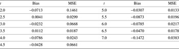
  $\overline{H}_{n}^{\beta} (f;t)$ using 250 bootstrap samples of size 20. Table 2 presents the bootstrap biases and mean-squared errors for the estimator
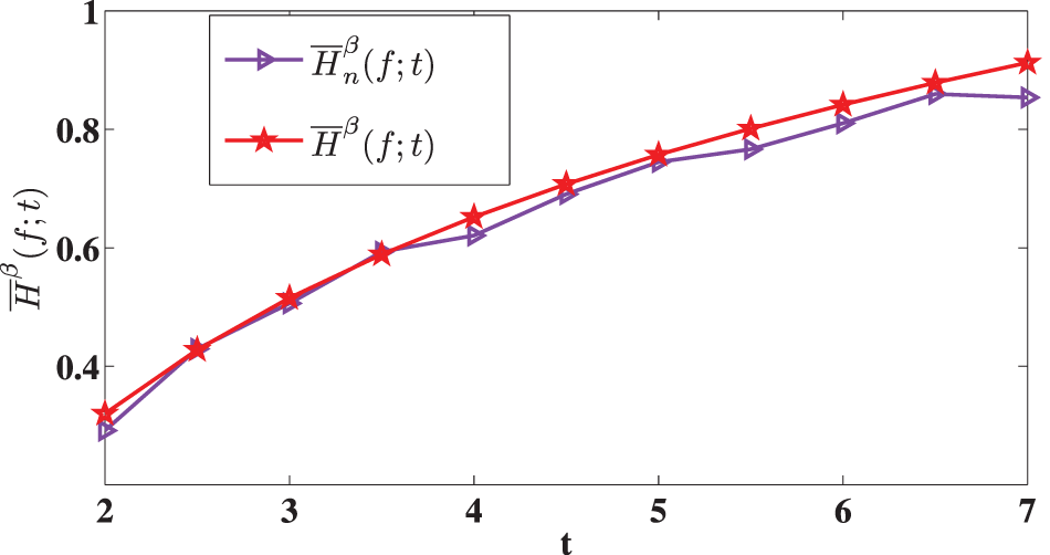
  $\overline{H}_{n}^{\beta} (f;t)$. Figure 1 compares the theoretical value $\overline{H}^{\beta} (f;t)$ with the estimated value $\overline{H}_n^{\beta} (f;t)$. From Figure 1, it is evident that for the given dataset, the generalized past entropy function increases over time.
Plots of estimates of generalized past entropy function for the first failure of 20 electric carts.

Bootstrap bias and mean-squared error of  $\overline H_{n}^{\beta}(f;t)$ for the real data set.

Next, we aim to examine the asymptotic normality of the estimator presented in Theorem 3.5. To achieve this, we conduct a numerical evaluation of  $\overline{H}^{\beta}_n (f;t)$ and analyze it through Monte Carlo simulations. Let $X$ follow an exponential distribution with parameter $\lambda$, where the mean is given by $\mu = 1/\lambda$. Then, the past entropy function of order $\beta$ is expressed as
 \begin{equation}
\overline H^{\beta} (f;t)=\frac{1}{1-\beta}\left[(\beta-1)\log\lambda-\log\beta-\beta\log(1-e^{-\lambda t})+\log(1-e^{-\lambda\beta t})\right].
\end{equation}
\begin{equation}
\overline H^{\beta} (f;t)=\frac{1}{1-\beta}\left[(\beta-1)\log\lambda-\log\beta-\beta\log(1-e^{-\lambda t})+\log(1-e^{-\lambda\beta t})\right].
\end{equation} Before obtaining our estimator, it is necessary to fix a function  $K$ and a sequence $\{b_n\}_{n\in\mathbb N}$ which satisfy the assumptions given in Section 2. Here, we consider
 \begin{eqnarray}
K(x)&=&\frac{1}{\sqrt{2\pi}}\exp\left(-\frac{x^2}{2}\right), \ \ x\in\mathbb R
\end{eqnarray}
\begin{eqnarray}
K(x)&=&\frac{1}{\sqrt{2\pi}}\exp\left(-\frac{x^2}{2}\right), \ \ x\in\mathbb R
\end{eqnarray} \begin{eqnarray}
b_n&=&\frac{1}{\sqrt{n}}, \ \ n\in\mathbb N.
\end{eqnarray}
\begin{eqnarray}
b_n&=&\frac{1}{\sqrt{n}}, \ \ n\in\mathbb N.
\end{eqnarray}By using these assumptions, we obtain
 \begin{equation*}
\nonumber
\Delta_K=\frac{1}{2\sqrt\pi},
\end{equation*}
\begin{equation*}
\nonumber
\Delta_K=\frac{1}{2\sqrt\pi},
\end{equation*}and, for the exponential distribution, we have
 \begin{equation*}
\nonumber
u(t)=\frac{\beta^2}{\lambda(\beta-1)}\frac{1-e^{-\lambda(\beta-1)t}}{1-e^{-\lambda\beta t}}.
\end{equation*}
\begin{equation*}
\nonumber
u(t)=\frac{\beta^2}{\lambda(\beta-1)}\frac{1-e^{-\lambda(\beta-1)t}}{1-e^{-\lambda\beta t}}.
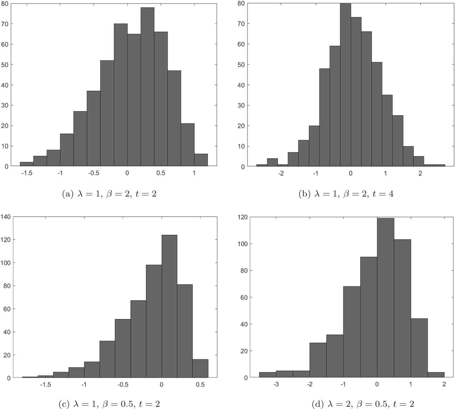
\end{equation*} We aim to verify whether the quantity defined in (3.15) follows a standard normal distribution. Using the exprnd function in MATLAB, we generate 500 samples, each of size  $N = 50$, from an exponential distribution with parameter $\lambda$. For each simulated sample, we extract only the values that do not exceed a fixed threshold $t$, and the count of these selected values is used as $n$ in our evaluations. Subsequently, using the fixed parameters, we compute the quantity given in (3.15) for each sample. To assess its asymptotic normality, we construct a histogram based on the 500 computed values. Specifically, we explore various choices for $\lambda$, $\beta$, and $t$, as illustrated in Figure 2.


6. Conclusion
This paper examines non-parametric estimators for the generalized past entropy function using kernel-based estimation, with  $\alpha$-mixing dependent observations. The asymptotic properties of the proposed estimator are analyzed and established. Additionally, a simulation study and real data analysis are carried out to evaluate the performance of the proposed estimator. We obtained that the estimator is performing good on both simulation study and data analysis owing to bias and $MSE$. As discussed earlier these estimate can be used in selecting a reliable system from the other available competing models.
Future research will extend beyond the  $\alpha$-mixing dependence condition to explore the inferential properties of generalized past entropy function under $\phi$-mixing and $\rho$-mixing dependence conditions.
Declaration of interests
The authors declare that they have no known competing financial interests or personal relationships that could have appeared to influence the work reported in this paper.
Acknowledgements
Francesco Buono and Maria Longobardi are members of the research group GNAMPA of INdAM (Istituto Nazionale di Alta Matematica). ML has been partially supported by MIUR—PRIN 2022 PNRR, project “Stochastic Modeling of Compound Events”, no. P2022KZJTZ, funded by European Union—Next Generation EU.
Appendix
R-code to find  $\overline H^{\beta}_n (f;t)$ by simulation for size $n$=100.
rm(list = ls())
library(MASS)
library(extremefit)
library(xlsx)
library(stats)
# Upper limit of integration
t <- 1
# PDF of the exponential distribution with rate = 1.5
f <- function(x) {
dexp(x, rate = 1)
}
# CDF of the exponential distribution at t
F_t <- pexp(t, rate = 1)
betas <- c( 2,4, 6, 8, 10) # Add more beta values as needed
results_list <- list()
for (beta in betas) {
r2 <- NULL # Reset results for each beta
n <- 100
r <- 1000
t <- 1
Hhat <- numeric(r)
for (s in 1:r) {
print(c(beta, k, s))
#set.seed(10)
# Generate data for the process
lambda <- 1
phi <- 0.2
X <- numeric(n)
a <- numeric(n)
for (i in 2:(n + 1)) {
a[i] <- sample(c(0, rexp(1, lambda)), prob = c(phi, 1 - phi), size = 1)
X[i] <- phi * X[i - 1] + a[i]
}
X <- X[-1]
# Bandwidth estimation
h <- bw.SJ(X)
# The integrand function: (f(x) / F_t)^beta
integrand <- function(x) {
(f(x) / F_t)^beta
}
# Integrate the function from 0 to t, passing beta
integral_result <- integrate(integrand, lower = 0, upper = t)
# Extract the integral value
integral_value <- integral_result$value
# PDF approximation using a kernel density estimator
int <- function(x) {
fn <- numeric(length(x))
for (i in 1:length(x)) {
fn[i] <- mean(dnorm((x[i] - X) / h) / h)
}
return(fn)
}
# Compute the non-parametric CDF Fn(t)
compute_Fn <- function(data, t) {
integrate(Vectorize(int), lower = 0, upper = t)$value
}
# Compute the integral of f_n(x)^beta from 0 to t
compute_integral <- function(data, t, beta){
integrand <- function(x) int(x)^beta
integrate(Vectorize(integrand), lower = 0, upper = t)$value
}
# Function to compute H^beta_n(f; t)
H_beta_n <- function(data, t, beta) {
integral_value <- compute_integral(data, t, beta)
Fn_t <- compute_Fn(data, t)
result <- (log(integral_value) - beta * log(Fn_t))
return(result)
}
# Compute H^beta_n(f; t)
Hhat[s] <- (1 / (1 - beta)) * H_beta_n(X, t, beta)
}
# Compute the estimator and related metrics
est <- (1 / (1 - beta)) * log(integral_value)
H <- mean(Hhat)
Mse <- (est - Hhat)^2
bias <- H - est
MSE <- mean(Mse)
}


 Open access