


1. Introduction
In this paper, we are concerned with an open large-scale storage system with non-reliable file servers in a communication network. The overall storage capacity is assumed to be limited.
In the network considered, servers can break down randomly and when the disk of a given server breaks down, its files are lost, but can be retrieved on the other servers if copies are available. In order to ensure persistence, a duplication mechanism of files to other servers is then performed. The goal is for each file to have at least one copy available on one of the servers as long as possible. Furthermore, in order to use the bandwidth in an optimal way, there should not be too many copies of a given file so that the network can accommodate a large number of distinct files.
In the system considered here, if there is enough storage capacity, a file with one copy can be duplicated on the other servers aiming to guarantee persistence in the system and new files can be admitted to the system for storage, each with two copies, otherwise, if capacity does not allow the new files are rejected and the duplication is blocked.
The natural critical parameters of the network are  $(N,\mu_N,\lambda_N,\xi_N,{F}_{N})$ where N is the number of servers, µN is the failure rates of servers, λN the bandwidth allocated to files duplication, ξN is the bandwidth allocated to new files admission and ${F}_{N}$ the total storage capacity. In this paper, it will be assumed that the total capacity ${F}_{N}$ is proportional to N, that is
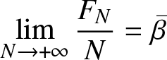 \begin{equation}
\lim_{N\rightarrow +\infty} \frac{{F}_{N}}{N} = {\bar{\beta}}
\end{equation}
\begin{equation}
\lim_{N\rightarrow +\infty} \frac{{F}_{N}}{N} = {\bar{\beta}}
\end{equation}  ${\bar{\beta}}$ is the average storage capacity per server, and that the parameters $\xi_N,\; \mu_N,\lambda_N$ are given by
 \begin{equation*}
\lambda_N = \lambda N,\quad \mu_N = \mu,\quad and \quad \xi_N = \xi N\end{equation*}
\begin{equation*}
\lambda_N = \lambda N,\quad \mu_N = \mu,\quad and \quad \xi_N = \xi N\end{equation*} for some positive real constants  $\lambda, \xi$ and µ.
The evolution in time of the number of files having one copy and files having two copies is modeled by two sequences of stochastic processes which are solutions of some stochastic differential equations with reflecting boundary. In order to study the qualitative behavior of the system, these stochastic processes are renormalized by a scaling parameter N. The resulting renormalized processes are the unique solution of a Skorokhod problem involving a sequence of random measures induced by the process describing the free capacity. Our main result shows that, as the scaling parameter goes to infinity, the sequence of renormalized processes is relatively compact in the space of  ${\mathbb{R}}^2$-valued right continuous functions on ${\mathbb{R}}_+$ with left limits and the limit of any convergent subsequence is the unique solution of a given deterministic dynamical system with reflections at the boundary of a bounded convex subset of ${\mathbb{R}}^2$ (Theorem 3.2). Without reflections at the boundary, this dynamical system admits a unique equilibrium point. According to the position of this equilibrium point, three possible regimes can therefore be derived: the under-loaded, the overloaded, and the critically loaded regime.
In the under-loaded regime, the probability of saturation of the system is small, and one can suppose that the capacity of the system is infinite and in this case the fluid limits are explicitly identified in El Kharroubi and El Masmari [Reference Kharroubi and Masmari7].
In the overloaded regime, the capacity  ${F}_{N}$ is reached in a finite time. In order to identify the fluid limits, exponential martingales are constructed which are useful in studying the limiting hitting time. Furthermore, the analysis involves a stochastic averaging principle with an underlying ergodic Markov process.
In the critically loaded regime, a probabilistic study of fluctuations of the processes around the equilibrium point gives the convergence to a reflected diffusion.
Large-scale storage networks of non-reliable file servers with duplication mechanism have been studied in many papers, see for example, Ramabhadran and Pasquale [Reference Ramabhadran and Pasquale12], Picconi, Baynat, and Sens [Reference Picconi, Baynat, Sens, Janowski and Mohanty9], Picconi et al. [Reference Picconi, Baynat and Sens10], Li, Ma, and Ma [Reference Quan-Lin, Fu-Qing and Jin-Yi11], and Aghajani, Robert, and Sun [Reference Aghajani, Robert and Sun1] where the impact of different replicating functionalities in a distributed system on its reliability is investigated using the theory of Markov processes. The present paper is one of the research articles on the stochastic analysis of unreliable storage systems with duplication mechanisms. The series of articles on this type of research began with the fundamental paper Feuillet and Robert [Reference Feuillet and Robert3], in which the authors investigated the evolution of a closed loss storage system and employed different time scales to provide an asymptotic description of the network’s decay. This work was generalized in Sun, Feuillet, and Robert [Reference Sun, Feuillet and Robert14], where the total number of replicas allowed for any file was assumed to be any integer d.
Within the same context, a recent paper El Kharroubi and El Masmari [Reference Kharroubi and Masmari7] investigated the storage system of non-reliable file servers with the duplication policy as an open network due to the newly added transition of admitting new files to the system. The asymptotic behavior of the system is studied under a fluid level, and the explicit expression of the associated fluid limits is obtained by solving a Skorokhod problem in the orthant  ${\mathbb{R}}_2^+$. Nevertheless, in El Kharroubi and El Masmari [Reference Kharroubi and Masmari7] capacity of the system is assumed to be infinite. And in order to give a complete description of a storage network with loss, duplication, and admitting policies which is of real use in practice, in this paper, capacity of the system is assumed to be finite and the asymptotic behavior of the system is also studied under a fluid level. The associated fluid limits are solutions of a Skorokhod problem in a given bounded convex domain in ${\mathbb{R}}_+^2$. Unfortunately, the resolution of the obtained Skorokhod problem is more complex due to the introduction of the process describing the free capacity of the system noted $(m^N(t))$.
Outline of the paper
Section 2 introduces the stochastic model considered and establishes the stochastic evolution equations of the Markov processes investigated. In Section 3, the link between the fluid equations and the Skorokhod problem is established. It is shown in Theorem 3.2 that the sequence of the scaled processes converges in distribution to a deterministic function, which is the unique solution of a given Skorokhod problem. The under-loaded regime and the critically loaded regimes are studied in Sections 4 and 6. In Section 5, the overloaded regime is investigated.
2. Stochastic model
In this paper, we consider a large-scale storage system that consists of N servers in a communication network. Let FN be the total number of files that can be stored in these servers. It will be assumed that FN is finite. The file storage system operates as follows: As long as the storage capacity is not exceeded new files can be admitted and files with one copy can be duplicated.
For  $i\in\{1,2\}$, $X_i^N (t)$ denotes the number of files with i copies present in the network at time t and $(X_0(t))$ denotes the number of files lost for good. Let $(m^N(t))$ be the number of free places in the network at time $t\geq 0$. The sequence of the processes $(m^N(t))$ is defined on $\bar{\mathbb{N}}=\mathbb{N}\cup \{+\infty\}$ and is given by
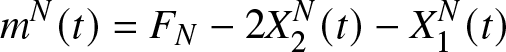 \begin{equation}
m^N(t)=F_{N}-2X_{2}^N (t)-X_{1}^N (t)
\end{equation}
\begin{equation}
m^N(t)=F_{N}-2X_{2}^N (t)-X_{1}^N (t)
\end{equation} The file duplication and admitting policies can be described as follows : conditionally on  $(X_{1}^{N} (t), X_2^N(t))=(x_1,x_2)$ with $x_1 \gt 0$ and $ 2x_2+x_1 \lt F_{N}$, a file with one copy gets an additional copy with rate $\frac{\lambda N}{x_1}$. If $m^N(t)\geq 2$, new files can be stored with rate $\xi N$. Copies of files disappear independently at rate µ. If the last replica of a given file is lost before being repaired, the file is then definitively lost.
All events are supposed to occur after an exponentially distributed time. The admitting, failure, and duplication processes are then independent Poisson processes. The process  ${X}^{N}(t)=(X_{1}^{N} (t),X_{2}^{N} (t))$ is then a Markov process on the state space
 \begin{equation*}
{\mathcal{D}}^N=\{(x_1,x_2)\in{\mathbb{N}}^2\;|\; 2x_2+x_1\leq {F}_{N} \}
\end{equation*}
\begin{equation*}
{\mathcal{D}}^N=\{(x_1,x_2)\in{\mathbb{N}}^2\;|\; 2x_2+x_1\leq {F}_{N} \}
\end{equation*} For  $(x_1,x_2) \in {\mathbb{N}}^{2}$ the ${\mathcal{Q}}$-matrix $Q^{N} = (q^{N}(.,.))$ of $({X}^{N}(t))$ is given by
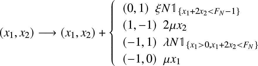 \begin{equation}
(x_1,x_2) \longrightarrow (x_1,x_2)+
\left\{ \begin{array}{ll}
(0,1) \ \ \xi N \mathbb{1}_{\lbrace x_1 + 2 x_2 \lt F_{N} -1 \rbrace} \\
(1,-1)\ \ 2 \mu x_2\\
(-1,1) \ \ \lambda N \mathbb{1}_{\lbrace x_1 \gt 0, x_1 + 2 x_2 \lt F_{N} \rbrace}\\
(-1,0) \ \ \mu x_1
\end{array}
\right.
\end{equation}
\begin{equation}
(x_1,x_2) \longrightarrow (x_1,x_2)+
\left\{ \begin{array}{ll}
(0,1) \ \ \xi N \mathbb{1}_{\lbrace x_1 + 2 x_2 \lt F_{N} -1 \rbrace} \\
(1,-1)\ \ 2 \mu x_2\\
(-1,1) \ \ \lambda N \mathbb{1}_{\lbrace x_1 \gt 0, x_1 + 2 x_2 \lt F_{N} \rbrace}\\
(-1,0) \ \ \mu x_1
\end{array}
\right.
\end{equation}2.1. Stochastic differential equations
The evolution equations associated to the Markov processes  $(X_{0}^{N}(t))$, $(X_{1}^{N}(t))$ and $(X_{2}^{N}(t))$ are given by:
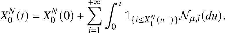 \begin{equation}
X_{0}^{N}(t) = X_{0}^N(0)+ \overset{+ \infty}{\underset{i = 1}{\sum }} \int_{0}^{t} \mathbb{1}_{\lbrace i \leq X_{1}^{N}(u^{-}) \rbrace} {\mathcal{N}}_{\mu,i}(du).
\end{equation}
\begin{equation}
X_{0}^{N}(t) = X_{0}^N(0)+ \overset{+ \infty}{\underset{i = 1}{\sum }} \int_{0}^{t} \mathbb{1}_{\lbrace i \leq X_{1}^{N}(u^{-}) \rbrace} {\mathcal{N}}_{\mu,i}(du).
\end{equation} \begin{eqnarray}
X_{1}^{N}(t)& = & X_{1}^{N}(0) - \int_{0}^{t} \mathbb{1}_{\lbrace X_{1}^{N}(u^{-}) \gt 0,2X_2^N(u^-)+X_1^N(u^-) \lt F_{N} \rbrace} {\mathcal{N}}_{\lambda N}(du)
\end{eqnarray}
\begin{eqnarray}
X_{1}^{N}(t)& = & X_{1}^{N}(0) - \int_{0}^{t} \mathbb{1}_{\lbrace X_{1}^{N}(u^{-}) \gt 0,2X_2^N(u^-)+X_1^N(u^-) \lt F_{N} \rbrace} {\mathcal{N}}_{\lambda N}(du)
\end{eqnarray}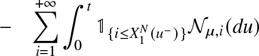 \begin{eqnarray*}
\nonumber &-& \overset{+ \infty}{\underset{i = 1}{\sum }} \int_{0}^{t} \mathbb{1}_{\lbrace i \leq X_{1}^{N}(u^{-}) \rbrace} {\mathcal{N}}_{\mu,i}(du)
\end{eqnarray*}
\begin{eqnarray*}
\nonumber &-& \overset{+ \infty}{\underset{i = 1}{\sum }} \int_{0}^{t} \mathbb{1}_{\lbrace i \leq X_{1}^{N}(u^{-}) \rbrace} {\mathcal{N}}_{\mu,i}(du)
\end{eqnarray*}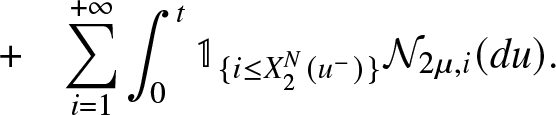 \begin{eqnarray*}
\nonumber
&+ &\overset{+ \infty}{\underset{i = 1}{\sum }} \int_{0}^{t} \mathbb{1}_{\lbrace i \leq X_{2}^{N}(u^{-}) \rbrace} {\mathcal{N}}_{2 \mu,i}(du).
\end{eqnarray*}
\begin{eqnarray*}
\nonumber
&+ &\overset{+ \infty}{\underset{i = 1}{\sum }} \int_{0}^{t} \mathbb{1}_{\lbrace i \leq X_{2}^{N}(u^{-}) \rbrace} {\mathcal{N}}_{2 \mu,i}(du).
\end{eqnarray*}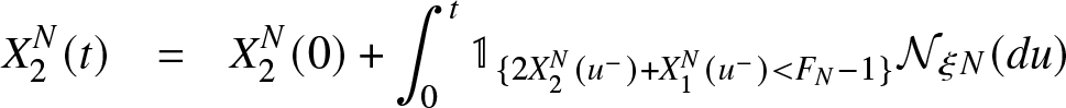 \begin{eqnarray}
X_{2}^{N}(t) &=& X_{2}^{N}(0) + \int_{0}^{t}\mathbb{1}_{\lbrace 2X_2^N(u^-)+X_1^N(u^-) \lt F_{N}-1 \rbrace}{\mathcal{N}}_{\xi N}(du)
\end{eqnarray}
\begin{eqnarray}
X_{2}^{N}(t) &=& X_{2}^{N}(0) + \int_{0}^{t}\mathbb{1}_{\lbrace 2X_2^N(u^-)+X_1^N(u^-) \lt F_{N}-1 \rbrace}{\mathcal{N}}_{\xi N}(du)
\end{eqnarray}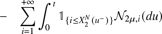 \begin{eqnarray*}
\nonumber
&-&\overset{+ \infty}{\underset{i = 1}{\sum }} \int_{0}^{t} \mathbb{1}_{\lbrace i \leq X_{2}^{N}(u^{-}) \rbrace} {\mathcal{N}}_{2 \mu,i}(du)
\end{eqnarray*}
\begin{eqnarray*}
\nonumber
&-&\overset{+ \infty}{\underset{i = 1}{\sum }} \int_{0}^{t} \mathbb{1}_{\lbrace i \leq X_{2}^{N}(u^{-}) \rbrace} {\mathcal{N}}_{2 \mu,i}(du)
\end{eqnarray*}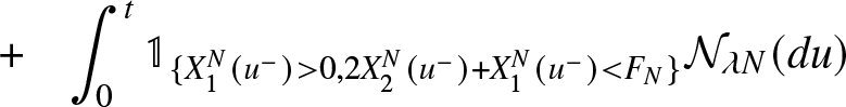 \begin{eqnarray*}
\nonumber
&+&\int_{0}^{t} \mathbb{1}_{\lbrace X_{1}^{N}(u^{-}) \gt 0, 2X_2^N(u^-)+X_1^N(u^-) \lt F_{N} \rbrace}{\mathcal{N}}_{\lambda N}(du)
\end{eqnarray*}
\begin{eqnarray*}
\nonumber
&+&\int_{0}^{t} \mathbb{1}_{\lbrace X_{1}^{N}(u^{-}) \gt 0, 2X_2^N(u^-)+X_1^N(u^-) \lt F_{N} \rbrace}{\mathcal{N}}_{\lambda N}(du)
\end{eqnarray*} where  $({\mathcal{N}}_{\alpha,i})$ denotes an i.i.d sequence of Poisson processes with parameter α. All the sequences of Poisson processes are assumed to be independent. And $x(u^-)=\lim\limits_{\substack{s\to u \\ s \lt u}}x(s) $
The equations (5) and (6) can be rewritten as
 \begin{align}
X_{1}^{N}(t) &= X_{1}^{N}(0)+ {M}_{1}^{N}(t) -\mu \int_{0}^{t} X_{1}^{N}(u) du +2\mu \int_{0}^{t} X_2^{N}(u) du
\end{align}
\begin{align}
X_{1}^{N}(t) &= X_{1}^{N}(0)+ {M}_{1}^{N}(t) -\mu \int_{0}^{t} X_{1}^{N}(u) du +2\mu \int_{0}^{t} X_2^{N}(u) du
\end{align}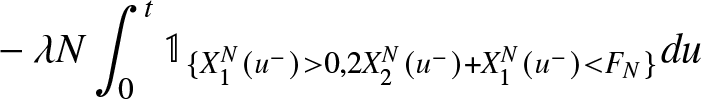 \begin{align*}
\nonumber
& -\lambda N \int_{0}^{t} \mathbb{1}_{\lbrace X_{1}^{N}(u^{-}) \gt 0,2X_2^N(u^-)+X_1^N(u^-) \lt F_{N} \rbrace} du
\end{align*}
\begin{align*}
\nonumber
& -\lambda N \int_{0}^{t} \mathbb{1}_{\lbrace X_{1}^{N}(u^{-}) \gt 0,2X_2^N(u^-)+X_1^N(u^-) \lt F_{N} \rbrace} du
\end{align*} \begin{align}
X_2^N(t)&=X_2^N(0)+ {M}_{2}^{N}(t)-2\mu \int_{0}^{t} X_2^{N}(u) du
\end{align}
\begin{align}
X_2^N(t)&=X_2^N(0)+ {M}_{2}^{N}(t)-2\mu \int_{0}^{t} X_2^{N}(u) du
\end{align} \begin{align*}
\nonumber
&+ \xi N \int_{0}^{t} \mathbb{1}_{\{2X_2^N(u^-)+X_1^N(u^-) \lt F_{N}-1\}} du\\
\nonumber
& +\lambda N \int_{0}^{t}\mathbb{1}_{\lbrace X_{1}^{N}(u^{-}) \gt 0,2X_2^N(u^-)+X_1^N(u^-) \lt F_{N} \rbrace}du \nonumber
\end{align*}
\begin{align*}
\nonumber
&+ \xi N \int_{0}^{t} \mathbb{1}_{\{2X_2^N(u^-)+X_1^N(u^-) \lt F_{N}-1\}} du\\
\nonumber
& +\lambda N \int_{0}^{t}\mathbb{1}_{\lbrace X_{1}^{N}(u^{-}) \gt 0,2X_2^N(u^-)+X_1^N(u^-) \lt F_{N} \rbrace}du \nonumber
\end{align*} where  $({M}_1^N(t))$ and $({M}_2^N(t))$ are martingales associated to Markov processes $(X_{1}^{N}(t))$ and $(X_{2}^{N}(t))$ (see[Reference Robert13] pp 348) given by :
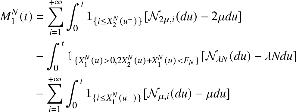 \begin{equation}
\begin{aligned}
{M}_{1}^{N}(t) &= \overset{+ \infty}{\underset{i = 1}{\sum }} \int_{0}^{t} \mathsf{1}_{\lbrace i \leq X_{2}^{N}(u^{-}) \rbrace} [ {\mathcal{N}}_{2 \mu,i}(du) -2 \mu du] \\
&- \int_{0}^{t} \mathbb{1}_{\{X_1^N(u) \gt 0,2X_2^N(u)+X_1^N(u) \lt F_{N}\}} [ {\mathcal{N}}_{\lambda N}(du) - \lambda N du ]\\
&- \overset{+ \infty}{\underset{i = 1}{\sum }} \int_{0}^{t} \mathsf{1}_{\lbrace i \leq X_{1}^{N}(u^{-}) \rbrace} [ {\mathcal{N}}_{\mu,i}(du) - \mu du]
\end{aligned}
\end{equation}
\begin{equation}
\begin{aligned}
{M}_{1}^{N}(t) &= \overset{+ \infty}{\underset{i = 1}{\sum }} \int_{0}^{t} \mathsf{1}_{\lbrace i \leq X_{2}^{N}(u^{-}) \rbrace} [ {\mathcal{N}}_{2 \mu,i}(du) -2 \mu du] \\
&- \int_{0}^{t} \mathbb{1}_{\{X_1^N(u) \gt 0,2X_2^N(u)+X_1^N(u) \lt F_{N}\}} [ {\mathcal{N}}_{\lambda N}(du) - \lambda N du ]\\
&- \overset{+ \infty}{\underset{i = 1}{\sum }} \int_{0}^{t} \mathsf{1}_{\lbrace i \leq X_{1}^{N}(u^{-}) \rbrace} [ {\mathcal{N}}_{\mu,i}(du) - \mu du]
\end{aligned}
\end{equation}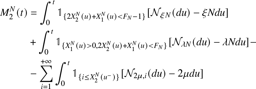 \begin{equation}
\begin{aligned}
{M}_{2}^{N}(t) &= \int_{0}^{t} \mathbb{1}_{\lbrace 2X_2^N(u)+X_1^N(u) \lt F_{N}-1\rbrace}[ {\mathcal{N}}_{\xi N}(du) - \xi N du ] \\
&+\int_{0}^{t} \mathbb{1}_{\{X_1^N(u) \gt 0,2X_2^N(u)+X_1^N(u) \lt F_{N}\}} [ {\mathcal{N}}_{\lambda N}(du) - \lambda N du ] -\\
&-\overset{+ \infty}{\underset{i = 1}{\sum }} \int_{0}^{t} \mathbb{1}_{\lbrace i \leq X_{2}^{N}(u^{-}) \rbrace} [ {\mathcal{N}}_{2 \mu,i}(du) - 2 \mu du]
\end{aligned}
\end{equation}
\begin{equation}
\begin{aligned}
{M}_{2}^{N}(t) &= \int_{0}^{t} \mathbb{1}_{\lbrace 2X_2^N(u)+X_1^N(u) \lt F_{N}-1\rbrace}[ {\mathcal{N}}_{\xi N}(du) - \xi N du ] \\
&+\int_{0}^{t} \mathbb{1}_{\{X_1^N(u) \gt 0,2X_2^N(u)+X_1^N(u) \lt F_{N}\}} [ {\mathcal{N}}_{\lambda N}(du) - \lambda N du ] -\\
&-\overset{+ \infty}{\underset{i = 1}{\sum }} \int_{0}^{t} \mathbb{1}_{\lbrace i \leq X_{2}^{N}(u^{-}) \rbrace} [ {\mathcal{N}}_{2 \mu,i}(du) - 2 \mu du]
\end{aligned}
\end{equation} The predictable increasing processes associated to the martingales  $({M}_{1}^{N}(t))$ and $({M}_{2}^{N}(t))$ are, respectively, given by
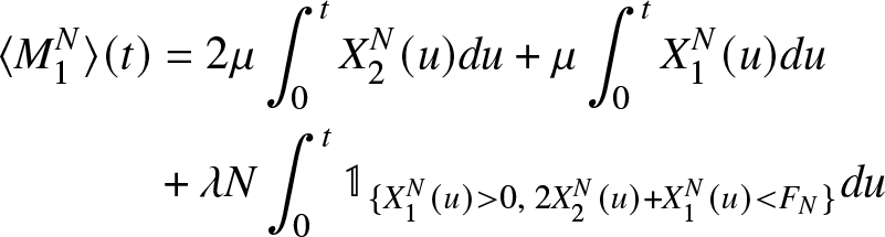 \begin{equation}\begin{aligned}
\langle {M}_{1}^{N}\rangle(t) &= 2 \mu \int_{0}^{t} X_{2}^{N}(u) du + \mu \int_{0}^{t} X_{1}^{N}(u) du \\
&+ \lambda N \int_{0}^{t}\mathbb{1}_{\lbrace X_{1}^{N}(u) \gt 0,\; 2X_2^N(u)+X_1^N(u) \lt F_{N} \rbrace} du
\end{aligned}
\end{equation}
\begin{equation}\begin{aligned}
\langle {M}_{1}^{N}\rangle(t) &= 2 \mu \int_{0}^{t} X_{2}^{N}(u) du + \mu \int_{0}^{t} X_{1}^{N}(u) du \\
&+ \lambda N \int_{0}^{t}\mathbb{1}_{\lbrace X_{1}^{N}(u) \gt 0,\; 2X_2^N(u)+X_1^N(u) \lt F_{N} \rbrace} du
\end{aligned}
\end{equation}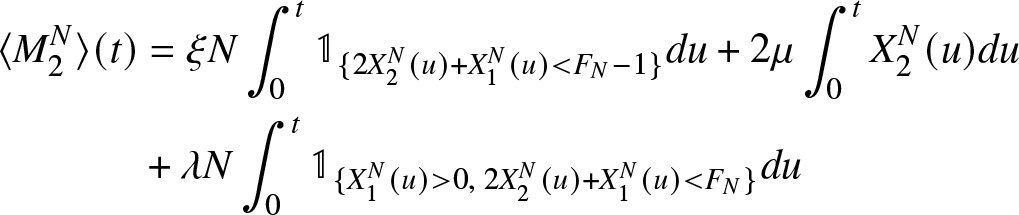 \begin{equation}
\begin{aligned}
\langle {M}_{2}^{N}\rangle(t)& = \xi N \int_{0}^{t} \mathbb{1}_{\lbrace 2X_2^N(u)+X_1^N(u) \lt F_{N}-1 \rbrace} du +2 \mu \int_{0}^{t} X_{2}^{N}(u) du\\
& + \lambda N \int_{0}^{t}\mathbb{1}_{\lbrace X_{1}^{N}(u) \gt 0,\;2X_2^N(u)+X_1^N(u) \lt F_{N} \rbrace} du
\end{aligned}
\end{equation}
\begin{equation}
\begin{aligned}
\langle {M}_{2}^{N}\rangle(t)& = \xi N \int_{0}^{t} \mathbb{1}_{\lbrace 2X_2^N(u)+X_1^N(u) \lt F_{N}-1 \rbrace} du +2 \mu \int_{0}^{t} X_{2}^{N}(u) du\\
& + \lambda N \int_{0}^{t}\mathbb{1}_{\lbrace X_{1}^{N}(u) \gt 0,\;2X_2^N(u)+X_1^N(u) \lt F_{N} \rbrace} du
\end{aligned}
\end{equation}3. Fluid equations and Skorokhod problem
Let  ${\mathcal{S}}$ be the convex domain in $ {\mathbb{R}}^2$ given by
 \begin{equation*}{\mathcal{S}}=\{(x_1,x_2)\in{\mathbb{R}}^2 |x_1\geq 0,x_2\geq 0, 2x_2+x_1\leq {\bar{\beta}}\}\end{equation*}
 and  $\mathcal{D}({\mathbb{R}}_+,{\mathbb{R}}^2)$ the space of ${\mathbb{R}}^2$-valued right continuous functions on ${\mathbb{R}}_+$ with left limits. Let ${\mathcal{M}}_{m,n}(\mathbb{R})$ be the space of m × n matrices over $\mathbb{R}$.
In this paper, we consider the following Skorokhod problem in the convex domain  ${\mathcal{S}}$. Let $\theta\in{\mathcal{M}}_{2,1}(\mathbb{R})$, $A\in{\mathcal{M}}_{2,2}(\mathbb{R})$ and $ R\in{\mathcal{M}}_{2,2}(\mathbb{R})$. Let ν be the measure on
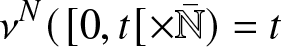
  $[0,+\infty[\times \bar{\mathbb{N}}$ satisfying $\nu([0,t]\times \bar{\mathbb{N}})=t$ for all $t\geq 0$.
Definition 3.1. The couple of functions  $z\in\mathcal{D}({\mathbb{R}}_+,{\mathbb{R}}^2)$ and $y\in\mathcal{D}({\mathbb{R}}_+,{\mathbb{R}}^2)$ with $z(0)\in {\mathcal{S}}$, is called the solution of the Skorokhod problem associated with the data $(\theta,\nu,A,R,{\mathcal{S}})$ and the function
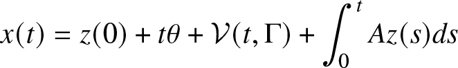 \begin{equation}
x(t)= z(0)+t\theta+\mathcal{V}(t,\Gamma)+\int_{0}^t Az(s)ds
\end{equation}
\begin{equation}
x(t)= z(0)+t\theta+\mathcal{V}(t,\Gamma)+\int_{0}^t Az(s)ds
\end{equation} where for Γ in a σ-algebra  $\mathcal{B}(\bar{\mathbb{N}})$
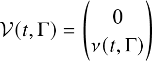 \begin{equation*}\mathcal{V}(t,\Gamma)=\begin{pmatrix} 0\\\nu(t,\Gamma)\end{pmatrix}\end{equation*}
if the three following conditions hold :
(1)
(14) \begin{equation}
z(t)=z(0)+t\theta+\mathcal{V}(t,\Gamma)+\int_{0}^t Az(s)ds+Ry(t)
\end{equation}
\begin{equation}
z(t)=z(0)+t\theta+\mathcal{V}(t,\Gamma)+\int_{0}^t Az(s)ds+Ry(t)
\end{equation}(2)
$z(t)\in {\mathcal{S}}$ for all
$t\geq 0$(3) for
$i=1,2$ the component yi of the function y are non-decreasing functions with
$y_i(0)=0$, and for
$t\geq 0$
(15)\begin{align}
&y_1(t)=\int_{0}^{t}\mathbb{1}_{\{z_1(s)=0\}} dy_1(s)
\end{align}(16)\begin{align}
&y_2(t)=\int_{0}^{t}\mathbb{1}_{\{z_1 \gt 0,z_1(s)+2z_2(s)={\bar{\beta}}\}} dy_2(s)
\end{align}


If  $z\in\mathcal{D}({\mathbb{R}}_+,{\mathbb{R}}^d)$ and $y\in\mathcal{D}({\mathbb{R}}_+,{\mathbb{R}}^d)$ with $z(0)\in {\mathcal{S}}$ is a solution of the above Skorokhod problem then the function $z=(z(t))$ has the following properties. First z behaves on the interior of the set S like a solution of the following ordinary differential equation
 \begin{equation}
x(t)=x(0)+\theta t+\mathcal{V}(t,\Gamma)+\int_0^t Ax(s)ds
\end{equation}
\begin{equation}
x(t)=x(0)+\theta t+\mathcal{V}(t,\Gamma)+\int_0^t Ax(s)ds
\end{equation} And second, z is reflected instantaneously at the boundaries  $(\partial{\mathcal{S}})_1=\{x_1=0\}$ and $(\partial{\mathcal{S}})_2=\{x_1+2x_2={\bar{\beta}}\}$ of the set ${\mathcal{S}}$. The direction of the reflection on the boundary $(\partial{\mathcal{S}})_1$ is the first column vector of the reflection matrix R and the direction of reflection on $(\partial{\mathcal{S}})_2$ is the second column vector the matrix R. See for example, Tanaka[Reference Tanaka15].
3.1. Fluid equations
If  $({X}^N(t))$ is a sequence of processes, one defines the renormalized sequence of processes of $({X}^N(t))$ by
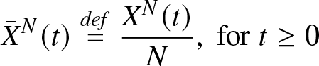 \begin{equation*}
{\bar{X}}^N(t)\stackrel{def}{=} \frac{{X}^{N}(t)}{N},\; \text{for}\; t\geq 0\end{equation*}
\begin{equation*}
{\bar{X}}^N(t)\stackrel{def}{=} \frac{{X}^{N}(t)}{N},\; \text{for}\; t\geq 0\end{equation*} From equations (2), (7), (8) one gets the fluid stochastic differential equations associated with the sequence of processes  $({\bar{X}}_1^N(t))$ and $({\bar{X}}_2^N(t))$
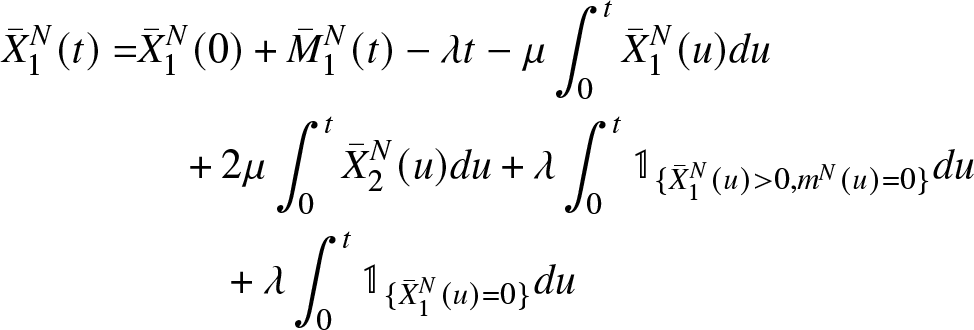 \begin{equation}
\begin{aligned}
{\bar{X}}_{1}^{N}(t) = & {\bar{X}}_{1}^{N}(0)+ {\bar{M}}_{1}^{N}(t)-\lambda t-\mu \int_{0}^{t} {\bar{X}}_{1}^{N}(u) du \\
&\quad +2\mu \int_{0}^{t} {\bar{X}}_2^{N}(u) du + \lambda \int_{0}^{t} \mathbb{1}_{\lbrace {\bar{X}}_{1}^{N}(u) \gt 0, m^N(u)=0\rbrace} du \\
&\qquad+\lambda \int_{0}^{t} \mathbb{1}_{\lbrace {\bar{X}}_{1}^{N}(u)=0\rbrace} du
\end{aligned}\end{equation}
\begin{equation}
\begin{aligned}
{\bar{X}}_{1}^{N}(t) = & {\bar{X}}_{1}^{N}(0)+ {\bar{M}}_{1}^{N}(t)-\lambda t-\mu \int_{0}^{t} {\bar{X}}_{1}^{N}(u) du \\
&\quad +2\mu \int_{0}^{t} {\bar{X}}_2^{N}(u) du + \lambda \int_{0}^{t} \mathbb{1}_{\lbrace {\bar{X}}_{1}^{N}(u) \gt 0, m^N(u)=0\rbrace} du \\
&\qquad+\lambda \int_{0}^{t} \mathbb{1}_{\lbrace {\bar{X}}_{1}^{N}(u)=0\rbrace} du
\end{aligned}\end{equation}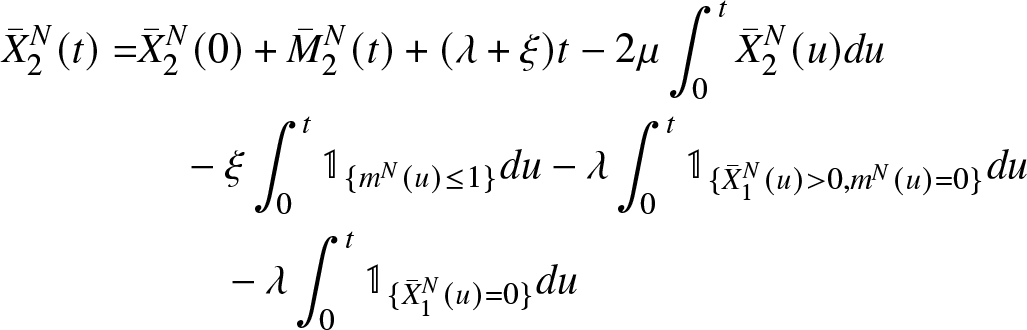 \begin{equation}
\begin{aligned}
{\bar{X}}_2^N(t) =& {\bar{X}}_2^N(0) + {\bar{M}}_{2}^{N}(t)+(\lambda+\xi)t-2\mu \int_{0}^{t} {\bar{X}}_2^{N}(u) du\\
&\quad -\xi \int_{0}^{t} \mathbb{1}_{\{m^N(u)\leq 1\}} du
-\lambda \int_{0}^{t} \mathbb{1}_{\lbrace {\bar{X}}_{1}^{N}(u) \gt 0 ,m^N(u)=0\rbrace} du\\
&\qquad- \lambda \int_{0}^{t} \mathbb{1}_{\lbrace {\bar{X}}_{1}^{N}(u)= 0\rbrace} du
\end{aligned}
\end{equation}
\begin{equation}
\begin{aligned}
{\bar{X}}_2^N(t) =& {\bar{X}}_2^N(0) + {\bar{M}}_{2}^{N}(t)+(\lambda+\xi)t-2\mu \int_{0}^{t} {\bar{X}}_2^{N}(u) du\\
&\quad -\xi \int_{0}^{t} \mathbb{1}_{\{m^N(u)\leq 1\}} du
-\lambda \int_{0}^{t} \mathbb{1}_{\lbrace {\bar{X}}_{1}^{N}(u) \gt 0 ,m^N(u)=0\rbrace} du\\
&\qquad- \lambda \int_{0}^{t} \mathbb{1}_{\lbrace {\bar{X}}_{1}^{N}(u)= 0\rbrace} du
\end{aligned}
\end{equation} The process  $(m^N(t))$ evolves on a very rapid time-scale compared with the process ${\bar{X}}^N(t)\stackrel{def}{=}( {\bar{X}}_1^N(t), {\bar{X}}_2^N(t))$. One can see that, while the velocity of the process $({\overline{X}}^N(t))$ is of the order O(1), the velocity of the process $(m^N(t))$ is much faster than $({\overline{X}}^N(t))$ and is of the order O(N).
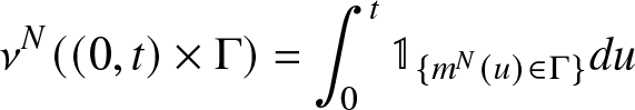
We consider as in Hunt and Kurtz [Reference Hunt and Kurtz5] the random measure ν N on  $[0,+\infty[\times \bar{\mathbb{N}}$ defined by
 \begin{equation}
\nu^N((0,t)\times \Gamma)=\int_0^t\mathbb{1}_{\{m^N(u)\in\Gamma\}}du
\end{equation}
\begin{equation}
\nu^N((0,t)\times \Gamma)=\int_0^t\mathbb{1}_{\{m^N(u)\in\Gamma\}}du
\end{equation} for all  $t\in [0,+\infty[$ and Γ in a σ-algebra $\mathcal{B}(\bar{\mathbb{N}})$. Note that the measure ν N satisfies the condition $\nu^N((0,t)\times \bar{\mathbb{N}})=t$. There is a subsequence of the sequence $(\nu^N)$ that converges in distribution to random measure ν satisfying $\nu((0,t)\times ~\bar{\mathbb{N}})=t$. (see Hunt and Kurtz [Reference Hunt and Kurtz5] for more details). In terms of the random measure ν N equations (18), (19) becomes
 \begin{equation}
\begin{aligned}
{\bar{X}}_{1}^{N}(t) = & {\bar{X}}_{1}^{N}(0)+ {\bar{M}}_{1}^{N}(t)-\lambda t-\mu \int_{0}^{t} {\bar{X}}_{1}^{N}(u) du \\
&\quad +2\mu \int_{0}^{t} {\bar{X}}_2^{N}(u) du + \lambda \int_{0}^{t} \mathbb{1}_{\lbrace {\bar{X}}_{1}^{N}(u) \gt 0, m^N(u)=0\rbrace} du \\
&\qquad+\lambda \int_{0}^{t} \mathbb{1}_{\lbrace {\bar{X}}_{1}^{N}(u)=0\rbrace} du
\end{aligned}
\end{equation}
\begin{equation}
\begin{aligned}
{\bar{X}}_{1}^{N}(t) = & {\bar{X}}_{1}^{N}(0)+ {\bar{M}}_{1}^{N}(t)-\lambda t-\mu \int_{0}^{t} {\bar{X}}_{1}^{N}(u) du \\
&\quad +2\mu \int_{0}^{t} {\bar{X}}_2^{N}(u) du + \lambda \int_{0}^{t} \mathbb{1}_{\lbrace {\bar{X}}_{1}^{N}(u) \gt 0, m^N(u)=0\rbrace} du \\
&\qquad+\lambda \int_{0}^{t} \mathbb{1}_{\lbrace {\bar{X}}_{1}^{N}(u)=0\rbrace} du
\end{aligned}
\end{equation}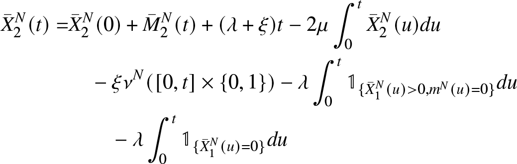 \begin{equation}
\begin{aligned}
{\bar{X}}_2^N(t) =& {\bar{X}}_2^N(0) + {\bar{M}}_{2}^{N}(t)+(\lambda+\xi)t-2\mu \int_{0}^{t} {\bar{X}}_2^{N}(u) du\\
&\quad -\xi \nu^N([0,t]\times\{0,1\})
-\lambda \int_{0}^{t} \mathbb{1}_{\lbrace {\bar{X}}_{1}^{N}(u) \gt 0 ,m^N(u)=0\rbrace} du\\
&\qquad- \lambda \int_{0}^{t} \mathbb{1}_{\lbrace {\bar{X}}_{1}^{N}(u)= 0\rbrace} du
\end{aligned}
\end{equation}
\begin{equation}
\begin{aligned}
{\bar{X}}_2^N(t) =& {\bar{X}}_2^N(0) + {\bar{M}}_{2}^{N}(t)+(\lambda+\xi)t-2\mu \int_{0}^{t} {\bar{X}}_2^{N}(u) du\\
&\quad -\xi \nu^N([0,t]\times\{0,1\})
-\lambda \int_{0}^{t} \mathbb{1}_{\lbrace {\bar{X}}_{1}^{N}(u) \gt 0 ,m^N(u)=0\rbrace} du\\
&\qquad- \lambda \int_{0}^{t} \mathbb{1}_{\lbrace {\bar{X}}_{1}^{N}(u)= 0\rbrace} du
\end{aligned}
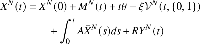
\end{equation}The above equations can be rewritten in the matrix form as follows:
 \begin{equation}
\begin{aligned}
{\bar{X}}^N(t)&={\bar{X}}^N(0)+{\bar{M}}^N(t)+t\bar{\theta}-\xi\mathcal{V}^N(t,\{0,1\})\\
&\qquad+ \int_{0}^t A{\bar{X}}^N(s)ds+RY^N(t)
\end{aligned}
\end{equation}
\begin{equation}
\begin{aligned}
{\bar{X}}^N(t)&={\bar{X}}^N(0)+{\bar{M}}^N(t)+t\bar{\theta}-\xi\mathcal{V}^N(t,\{0,1\})\\
&\qquad+ \int_{0}^t A{\bar{X}}^N(s)ds+RY^N(t)
\end{aligned}
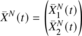
\end{equation}where
 \begin{equation*}
{\bar{X}}^N(t)=\begin{pmatrix}{\bar{X}}_{1}^{N}(t)\\ {\bar{X}}_{2}^N(t)\end{pmatrix}\; {\bar{M}}^N(t)=\begin{pmatrix} \frac{{M}_{1}^{N}(t)}{N}\\ \frac{{M}_{2}^{N}(t)}{N} \end{pmatrix}\end{equation*}
\begin{equation*}
{\bar{X}}^N(t)=\begin{pmatrix}{\bar{X}}_{1}^{N}(t)\\ {\bar{X}}_{2}^N(t)\end{pmatrix}\; {\bar{M}}^N(t)=\begin{pmatrix} \frac{{M}_{1}^{N}(t)}{N}\\ \frac{{M}_{2}^{N}(t)}{N} \end{pmatrix}\end{equation*}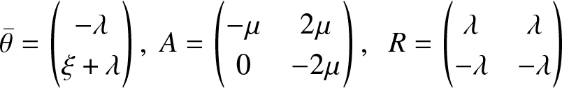 \begin{equation*}
\bar{\theta}=\begin{pmatrix} -\lambda\\\xi +\lambda\end{pmatrix},
\; A=\begin{pmatrix} -\mu & 2\mu \\ 0 & -2\mu \end{pmatrix},\;\; R=\begin{pmatrix} \lambda & \lambda\\ -\lambda & -\lambda\end{pmatrix}\end{equation*}
\begin{equation*}
\bar{\theta}=\begin{pmatrix} -\lambda\\\xi +\lambda\end{pmatrix},
\; A=\begin{pmatrix} -\mu & 2\mu \\ 0 & -2\mu \end{pmatrix},\;\; R=\begin{pmatrix} \lambda & \lambda\\ -\lambda & -\lambda\end{pmatrix}\end{equation*}
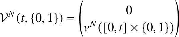 \begin{equation*}\mathcal{V}^N(t,\{0,1\})=\begin{pmatrix} \nonumber 0 \\ \nu^N([0,t] \times \{0,1\})\end{pmatrix}\end{equation*}
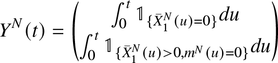 \begin{equation*} Y^N(t)=\begin{pmatrix}
\int_{0}^{t} \mathbb{1}_{\{{\bar{X}}_1^N(u)= 0\}}du\\
\int_{0}^{t} \mathbb{1}_{\lbrace {\bar{X}}_{1}^{N}(u) \gt 0 ,m^N(u)=0\rbrace} du\end{pmatrix}\end{equation*}
\begin{equation*} Y^N(t)=\begin{pmatrix}
\int_{0}^{t} \mathbb{1}_{\{{\bar{X}}_1^N(u)= 0\}}du\\
\int_{0}^{t} \mathbb{1}_{\lbrace {\bar{X}}_{1}^{N}(u) \gt 0 ,m^N(u)=0\rbrace} du\end{pmatrix}\end{equation*} As illustrated in Figure 1 the couple of processes  $( {\bar{X}}^N(t) )$ and $(Y^N (t))$ can be interpreted as the solution of the Skorokhod problem associated with data $(\bar{\theta} ,\nu^N, A,R,{\mathcal{S}})$ and
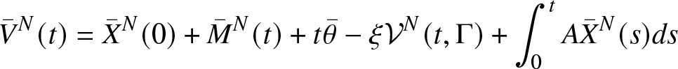 \begin{equation} {\bar{V}}^N(t)={\bar{X}}^N(0)+{\bar{M}}^N(t)+t\bar{\theta}-\xi\mathcal{V}^N(t,\Gamma)+ \int_{0}^t A{\bar{X}}^N(s)ds \end{equation}
 The following graphic illustrates the simulation for the process  $ ( {\overline{X}}_1(t), {\overline{X}}_2(t))$, and it has been shown that the process $ ( {\overline{X}}_1(t))$ is well reflected at the boundary ${(\partial{\mathcal{S}})}_1$ and the process $ ( {\overline{X}}_1(t) + 2 ( {\overline{X}}_2(t)) )$ is reflected at the boundary $(\partial{\mathcal{S}})_2$.
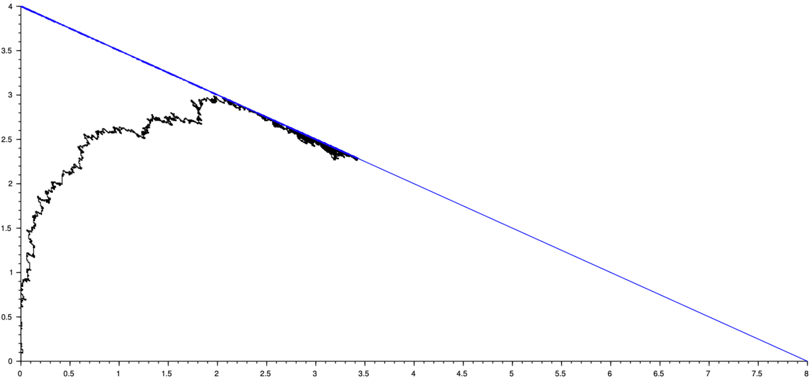
Figure 1. Simulation of the process  $({\overline{X}}_1^N(t), {\overline{X}}_2^N(t))$ in the convex ${\mathcal{S}}$
In the next theorem, we prove the relative compactness of the sequence of processes  $\left({\overline{X}}^{N}(.),Y^{N}(.), {\mathcal{V}}^N(.)\right)$ in $\mathcal{D}({\mathbb{R}}_+,{\mathbb{R}}^2)\times {\mathcal{M}}_{1}({\mathbb{R}}_+\times\bar{\mathbb{N}})$. Where ${\mathcal{M}}_{1}({\mathbb{R}}_+\times\bar{\mathbb{N}})$ is the space of Radon measures on ${\mathbb{R}}_+\times\bar{\mathbb{N}}$.
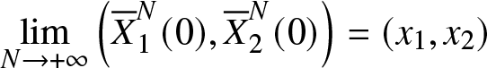
Theorem 3.2 Suppose that
 \begin{eqnarray*}
\nonumber \underset{N \rightarrow + \infty}{lim} ( {\overline{X}}_1^N(0), {\overline{X}}_2^N(0)) = (x_1, x_2) \in {\mathcal{S}},
\end{eqnarray*}
\begin{eqnarray*}
\nonumber \underset{N \rightarrow + \infty}{lim} ( {\overline{X}}_1^N(0), {\overline{X}}_2^N(0)) = (x_1, x_2) \in {\mathcal{S}},
\end{eqnarray*} the sequence  $\left({\overline{X}}^{N}(.),Y^{N}(.), \nu^N(.)\right)$ is then relatively compact in $\mathcal{D}({\mathbb{R}}_+,{\mathbb{R}}^3)$ and the limit $\left( x(.) ,y(.), \nu(.)\right)$ of any convergent subsequence satisfies:
 \begin{equation}
\begin{aligned}
x_1(t) &= x_1 - \lambda t-\mu \int_{0}^t x_1(s)ds + 2\mu \int_{0}^t x_2(s) ds \\
&+ \lambda \int_{[0,t] \times \mathbb{N}} \mathbb{1}_{\lbrace x_1(s) \gt 0 \rbrace} \mathbb{1}_{\lbrace 0 \rbrace} (u) \nu (ds \times du) +\lambda y_1(t)
\end{aligned}
\end{equation}
\begin{equation}
\begin{aligned}
x_1(t) &= x_1 - \lambda t-\mu \int_{0}^t x_1(s)ds + 2\mu \int_{0}^t x_2(s) ds \\
&+ \lambda \int_{[0,t] \times \mathbb{N}} \mathbb{1}_{\lbrace x_1(s) \gt 0 \rbrace} \mathbb{1}_{\lbrace 0 \rbrace} (u) \nu (ds \times du) +\lambda y_1(t)
\end{aligned}
\end{equation}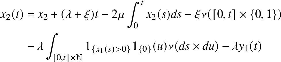 \begin{equation}
\begin{aligned}
x_2(t) &= x_2 + (\lambda+\xi) t -2 \mu \int_{0}^t x_2(s) ds- \xi \nu ([0,t] \times \{0,1\}) \\
& - \lambda \int_{[0,t] \times \mathbb{N}} \mathbb{1}_{\lbrace x_1(s) \gt 0 \rbrace} \mathbb{1}_{\lbrace 0 \rbrace} (u) \nu (ds \times du) - \lambda y_1(t)
\end{aligned}
\end{equation}
\begin{equation}
\begin{aligned}
x_2(t) &= x_2 + (\lambda+\xi) t -2 \mu \int_{0}^t x_2(s) ds- \xi \nu ([0,t] \times \{0,1\}) \\
& - \lambda \int_{[0,t] \times \mathbb{N}} \mathbb{1}_{\lbrace x_1(s) \gt 0 \rbrace} \mathbb{1}_{\lbrace 0 \rbrace} (u) \nu (ds \times du) - \lambda y_1(t)
\end{aligned}
\end{equation} where the function y1 is a non-decreasing function with  $y_1(0)=0$, and for $t\geq 0$
 \begin{equation*}\begin{aligned} y_1(t)=\int_{0}^{t}\mathbb{1}_{\{x_1(s)=0\}} dy_1(s)
\end{aligned}
\end{equation*}
\begin{equation*}\begin{aligned} y_1(t)=\int_{0}^{t}\mathbb{1}_{\{x_1(s)=0\}} dy_1(s)
\end{aligned}
\end{equation*}Lemma 3.3. The sequences of processes  $\left(\frac{{M}_{1}^{N}(t)}{N}\right)_{t\geq0}$ and $\left(\frac{{M}_{2}^{N}(t)}{N}\right)_{t\geq0}$ converge in distribution to 0 uniformly on compact sets.
Proof. Doob’s inequalities show that, for ϵ > 0 and  $t \geq 0$
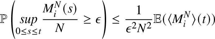 \begin{equation*}
\mathbb{P}\left( \underset{0 \leq s\leq t }{sup}\frac{{M}_{i}^{N}(s)}{N} \geq \epsilon \right)\leq \frac{1}{\epsilon^{2} N^{2}} \mathbb{E} ( \langle {M}_{i}^{N}\rangle(t))\end{equation*}
\begin{equation*}
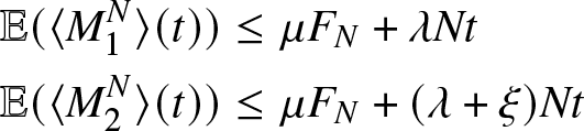
\mathbb{P}\left( \underset{0 \leq s\leq t }{sup}\frac{{M}_{i}^{N}(s)}{N} \geq \epsilon \right)\leq \frac{1}{\epsilon^{2} N^{2}} \mathbb{E} ( \langle {M}_{i}^{N}\rangle(t))\end{equation*}From equations (11), (12) one gets
 \begin{equation*}
\begin{aligned}
\mathbb{E} ( \langle {M}_{1}^{N}\rangle(t))&\leq \mu {F}_{N}+\lambda Nt\\
\mathbb{E} ( \langle {M}_{2}^{N}\rangle(t))&\leq \mu {F}_{N}+(\lambda+\xi) Nt\\
\end{aligned}
\end{equation*}
\begin{equation*}
\begin{aligned}
\mathbb{E} ( \langle {M}_{1}^{N}\rangle(t))&\leq \mu {F}_{N}+\lambda Nt\\
\mathbb{E} ( \langle {M}_{2}^{N}\rangle(t))&\leq \mu {F}_{N}+(\lambda+\xi) Nt\\
\end{aligned}
\end{equation*} Then from (1) the sequences of processes  $\left(\frac{{M}_{1}^{N}(t)}{N}\right)_{t\geq0}$ and $\left(\frac{{M}_{2}^{N}(t)}{N}\right)_{t\geq0}$ converge in distribution to 0 uniformly on any bounded time interval.
Proof. proof of Theorem 3.2
First, we prove the relative compactness of the process
 \begin{equation*}{\bar{X}}^N(t)=\begin{pmatrix}{\bar{X}}_{1}^{N}(t)\\ {\bar{X}}_{2}^N(t)\end{pmatrix}
\end{equation*}
\begin{equation*}{\bar{X}}^N(t)=\begin{pmatrix}{\bar{X}}_{1}^{N}(t)\\ {\bar{X}}_{2}^N(t)\end{pmatrix}
\end{equation*} For this we prove separately that $({\overline{X}}_1^{N}(t))$ and $({\overline{X}}_2^{N}(t))$ are tight.
For  $T \gt 0, \delta \gt 0$ we denote by $\omega_{g}^T(\delta)$ the modulus of continuity of the function g on $[0,T]$:
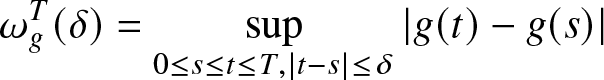 \begin{equation}
\omega_{g}^T(\delta)=\sup_{0\leq s\leq t\leq T,|t-s|\leq \delta}\vert g(t)-g(s)\vert
\end{equation}
\begin{equation}
\omega_{g}^T(\delta)=\sup_{0\leq s\leq t\leq T,|t-s|\leq \delta}\vert g(t)-g(s)\vert
\end{equation} The equation (21) shows that the processes  $({\overline{X}}_1^{N}(t),Y_1^N(t))$ with $Y_1^N(t)=\lambda\int_{0}^{t} \mathbb{1}_{\{X_1^N(u)= 0\}} du)$ is the unique solution of the Skorokhod problem associated to the process
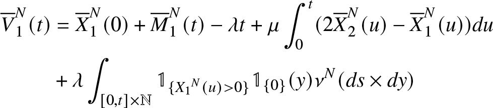 \begin{equation}\begin{aligned}
{\overline{V}}_1^N(t)& = {\overline{X}}_1^N(0) + {\overline{M}}_1^N(t) - \lambda t + \mu \int_{0}^t (2 {\overline{X}}_2^N(u) - {\overline{X}}_1^N(u) ) du \\
&+ \lambda \int_{[0,t] \times \mathbb{N}} \mathbb{1}_{\lbrace {X_1}^{N}(u) \gt 0 \rbrace}\mathbb{1}_{\lbrace 0 \rbrace} (y) \nu^N (ds \times dy)
\end{aligned}
\end{equation}
\begin{equation}\begin{aligned}
{\overline{V}}_1^N(t)& = {\overline{X}}_1^N(0) + {\overline{M}}_1^N(t) - \lambda t + \mu \int_{0}^t (2 {\overline{X}}_2^N(u) - {\overline{X}}_1^N(u) ) du \\
&+ \lambda \int_{[0,t] \times \mathbb{N}} \mathbb{1}_{\lbrace {X_1}^{N}(u) \gt 0 \rbrace}\mathbb{1}_{\lbrace 0 \rbrace} (y) \nu^N (ds \times dy)
\end{aligned}
\end{equation}By using explicit representation of the solution of the Skorokhod in dimension 1, see El Karoui and Chaleyat-Maurel [Reference Karoui and Chaleyat-Maurel6], one has
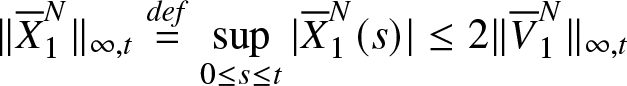 \begin{equation*} \|{\overline{X}}_1^N\|_{\infty,t}\stackrel{def}{=}\sup_{0\leq s\leq t}|{\overline{X}}_1^N(s)|\leq 2 \|{\overline{V}}_1^{N}\|_{\infty,t} \end{equation*}
and
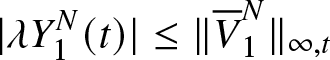 \begin{equation*}|\lambda Y_{1}^N(t)|\leq \|{\overline{V}}_1^{N}\|_{\infty,t}\end{equation*}
By equation (29), one gets that
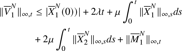 \begin{equation*}\begin{aligned}\nonumber
\|{\overline{V}}_1^{N}\|_{\infty,t}&\leq |{\overline{X}}_1^N(0))|+ 2 \lambda t+\mu \int_0^t\|{\overline{X}}_1^N\|_{\infty,s}ds\\ \nonumber
&+2\mu\int_0^t\|{\overline{X}}_2^N\|_{\infty,s}ds+ \|{\overline{M}}_1^{N}\|_{\infty,t}
\end{aligned}
\end{equation*}
\begin{equation*}\begin{aligned}\nonumber
\|{\overline{V}}_1^{N}\|_{\infty,t}&\leq |{\overline{X}}_1^N(0))|+ 2 \lambda t+\mu \int_0^t\|{\overline{X}}_1^N\|_{\infty,s}ds\\ \nonumber
&+2\mu\int_0^t\|{\overline{X}}_2^N\|_{\infty,s}ds+ \|{\overline{M}}_1^{N}\|_{\infty,t}
\end{aligned}
\end{equation*}and using inequalities given above,
 \begin{equation*}\begin{aligned}\nonumber
\|{\overline{X}}_1^N\|_{\infty,t}&\leq 2 |{\overline{X}}_1^N(0)|+4 \lambda t+2\mu\int_0^t\|{\overline{X}}_1^N\|_{\infty,s}ds\\ \nonumber
&+4\mu\int_0^t\|{\overline{X}}_2^N\|_{\infty,s}ds+ 2\|{\overline{M}}_1^{N}\|_{\infty,t}\nonumber
\end{aligned}
\end{equation*}
\begin{equation*}\begin{aligned}\nonumber
\|{\overline{X}}_1^N\|_{\infty,t}&\leq 2 |{\overline{X}}_1^N(0)|+4 \lambda t+2\mu\int_0^t\|{\overline{X}}_1^N\|_{\infty,s}ds\\ \nonumber
&+4\mu\int_0^t\|{\overline{X}}_2^N\|_{\infty,s}ds+ 2\|{\overline{M}}_1^{N}\|_{\infty,t}\nonumber
\end{aligned}
\end{equation*} \begin{equation*}\begin{aligned}\nonumber
\|{\overline{X}}_2^N\|_{\infty,t}&\leq |{\overline{X}}_1^N(0)|+|{\overline{X}}_2^N(0)|+(4\lambda+3\xi) t
+ \|{\overline{M}}_1^{N}\|_{\infty,t}+\|{\overline{M}}_2^{N}\|_{\infty,t}\\ \nonumber
&+\mu\int_0^t\|{\overline{X}}_1^N\|_{\infty,s}ds+4\mu\int_0^t\|{\overline{X}}_2^N\|_{\infty,s}ds
\end{aligned}
\end{equation*}
\begin{equation*}\begin{aligned}\nonumber
\|{\overline{X}}_2^N\|_{\infty,t}&\leq |{\overline{X}}_1^N(0)|+|{\overline{X}}_2^N(0)|+(4\lambda+3\xi) t
+ \|{\overline{M}}_1^{N}\|_{\infty,t}+\|{\overline{M}}_2^{N}\|_{\infty,t}\\ \nonumber
&+\mu\int_0^t\|{\overline{X}}_1^N\|_{\infty,s}ds+4\mu\int_0^t\|{\overline{X}}_2^N\|_{\infty,s}ds
\end{aligned}
\end{equation*}Then
 \begin{equation*}\nonumber
\|{\overline{X}}_1^N\|_{\infty,t}+\|{\overline{X}}_2^N\|_{\infty,t}\leq H^N(T)+8\mu\int_0^t(\|{\overline{X}}_1^N\|_{\infty,s}+\|{\overline{X}}_2^N\|_{\infty,s})ds
\end{equation*}
\begin{equation*}\nonumber
\|{\overline{X}}_1^N\|_{\infty,t}+\|{\overline{X}}_2^N\|_{\infty,t}\leq H^N(T)+8\mu\int_0^t(\|{\overline{X}}_1^N\|_{\infty,s}+\|{\overline{X}}_2^N\|_{\infty,s})ds
\end{equation*}with
 \begin{equation*}H^N(t)=3|{\overline{X}}_1^N(0)|+ |{\overline{X}}_2^N(0)|+(8\lambda+3\xi)T+3\|{\overline{M}}_1^{N}\|_{\infty,T}+\|{\overline{M}}_2^{N}\|_{\infty,T}\end{equation*}
Gronwall’s lemma gives that the relation
 \begin{equation*}\|{\overline{X}}_1^N\|_{\infty,t}+\|{\overline{X}}_2^N\|_{\infty,t}\leq H^N(T)e^{8\mu t}\end{equation*}
 holds for all  $t\in[0,T]$. The convergence of martingales and of $|{\overline{X}}_1^N(0)|$, $|{\overline{X}}_2^N(0)|$ shows that the sequence $(H^N(T))$ converges in distribution. Consequently for ϵ > 0, there exists some C > 0 such that for $i=1,2$ and all $N\in\mathbb{N}$
 \begin{equation*}\mathbb{P}\left(\|{\overline{X}}_1^N\|_{\infty,t} + \|{\overline{X}}_2^N\|_{\infty,t} \gt C\right)\leq \epsilon.
\end{equation*}
\begin{equation*}\mathbb{P}\left(\|{\overline{X}}_1^N\|_{\infty,t} + \|{\overline{X}}_2^N\|_{\infty,t} \gt C\right)\leq \epsilon.
\end{equation*} If η > 0, there exists N 1 and δ > 0 such that for all  $N\geq N_1$
 \begin{equation*}\delta(\lambda+4\mu C)\leq \frac{\eta}{2}\end{equation*}
and
 \begin{equation*}\mathbb{P}\left(\omega_{{\overline{M}}_{1}^{N}}^T(\delta)\geq \frac{\eta}{2}\right)\leq \epsilon\end{equation*}
One gets finally
 \begin{align*}
\mathbb{P}\left(\omega_{{\overline{V}}_{1}^{N}}^T(\delta)\geq \eta\right)&\leq\mathbb{P}\left(2\lambda\delta+2\mu\delta(\|{\overline{X}}_1^N\|_{\infty,T}+\|{\overline{X}}_2^N\|_{\infty,T})\geq \frac{\eta}{2}\right)\\
&+\mathbb{P}\left(\omega_{{\overline{M}}_{1}^{N}}^T(\delta)\geq \frac{\eta}{2}\right)\leq 3\epsilon
\end{align*}
\begin{align*}
\mathbb{P}\left(\omega_{{\overline{V}}_{1}^{N}}^T(\delta)\geq \eta\right)&\leq\mathbb{P}\left(2\lambda\delta+2\mu\delta(\|{\overline{X}}_1^N\|_{\infty,T}+\|{\overline{X}}_2^N\|_{\infty,T})\geq \frac{\eta}{2}\right)\\
&+\mathbb{P}\left(\omega_{{\overline{M}}_{1}^{N}}^T(\delta)\geq \frac{\eta}{2}\right)\leq 3\epsilon
\end{align*} Consequently the sequence  $({\overline{V}}_{1}^{N}(t))$ is tight and by continuity of the solution of the Skorokhod problem in dimension 1 the sequences $({\overline{X}}_1^N(t))$ and $(\overline{Y}_1^{N}(t))$ are tight, see Billingsley [Reference Patrick8].
From equation ((22)) one gets for s < t :
 \begin{equation*}
\begin{aligned}
\nonumber |{\overline{X}}_2^N(t)-{\overline{X}}_2^N(s)| &\leq (\lambda+\xi)(t-s)+2\mu\int_s^t|{\overline{X}}_2^N(u)|du+|{\overline{M}}_{2}^{N}(t)-{\overline{M}}_{2}^{N}(s)| \\ \nonumber
&+ (2\lambda+\xi)(t-s)+\lambda (Y_1^N(t)-Y_1^N(s))
\end{aligned}
\end{equation*}
\begin{equation*}
\begin{aligned}
\nonumber |{\overline{X}}_2^N(t)-{\overline{X}}_2^N(s)| &\leq (\lambda+\xi)(t-s)+2\mu\int_s^t|{\overline{X}}_2^N(u)|du+|{\overline{M}}_{2}^{N}(t)-{\overline{M}}_{2}^{N}(s)| \\ \nonumber
&+ (2\lambda+\xi)(t-s)+\lambda (Y_1^N(t)-Y_1^N(s))
\end{aligned}
\end{equation*}and
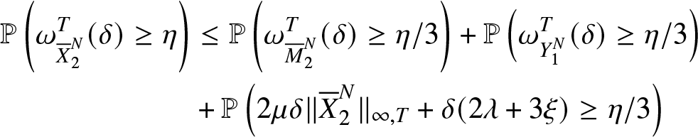 \begin{equation}
\begin{aligned}
\mathbb{P}\left(\omega_{{\overline{X}}_2^N}^T(\delta) \geq \eta\right) &\leq \mathbb{P}\left(\omega_{{\overline{M}}_{2}^{N}}^T(\delta)\geq \eta/3\right)
+\mathbb{P}\left(\omega_{Y_{1}^{N}}^T(\delta)\geq \eta/3\right)\\
&+\mathbb{P}\left(2\mu\delta\|{\overline{X}}_2^N\|_{\infty,T}+\delta(2 \lambda+3 \xi) \geq \eta/3\right)
\end{aligned}
\end{equation}
\begin{equation}
\begin{aligned}
\mathbb{P}\left(\omega_{{\overline{X}}_2^N}^T(\delta) \geq \eta\right) &\leq \mathbb{P}\left(\omega_{{\overline{M}}_{2}^{N}}^T(\delta)\geq \eta/3\right)
+\mathbb{P}\left(\omega_{Y_{1}^{N}}^T(\delta)\geq \eta/3\right)\\
&+\mathbb{P}\left(2\mu\delta\|{\overline{X}}_2^N\|_{\infty,T}+\delta(2 \lambda+3 \xi) \geq \eta/3\right)
\end{aligned}
\end{equation} There exists  $N_1\geq 0$ such that $\delta(2\mu C-\xi)\leq\epsilon$ and
 \begin{equation*}\mathbb{P}\left(\omega_{{\overline{M}}_{2}^{N}}^T(\delta)\geq \frac{\eta}{3}\right)\leq \epsilon\end{equation*}
and
 \begin{equation*}\mathbb{P}\left(\lambda\omega_{\frac{{Y}_{1}^{N}}{N}}^T(\delta)\geq \frac{\eta}{3}\right)\leq \epsilon\end{equation*}
and, consequently
 \begin{equation*}\mathbb{P}\left(\omega_{{\overline{X}}_2^N}^T(\delta)\geq \eta\right)\leq 3\epsilon\end{equation*}
 The sequence  ${\overline{X}}_2^N$ is therefore tight.
It remains to prove the relative compactness of the sequence of random measures ν N on  $[0,+\infty[\times\bar{\mathbb{N}}$. Since for all N and all $t\geq 0$
 \begin{equation*}
\nu^N([0,t[\times\bar{\mathbb{N}})=t\end{equation*}
\begin{equation*}
\nu^N([0,t[\times\bar{\mathbb{N}})=t\end{equation*}The result is given in Hunt and Kurtz [Reference Thomas17] Lemma 1.3.
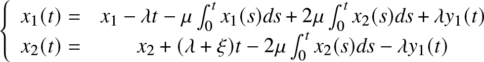
Remark 3.4. The dynamical system associated to the equations given in (25) and (26) are given by
 \begin{equation*}
\left\{\begin{array}{cc}
x_1(t)=&x_1-\lambda t-\mu\int_0^tx_1(s)ds+2\mu\int_0^tx_2(s)ds+\lambda y_1(t)\\
x_2(t)=&x_2+(\lambda+\xi) t-2\mu\int_0^tx_2(s)ds-\lambda y_1(t)
\end{array}
\right.
\end{equation*}
\begin{equation*}
\left\{\begin{array}{cc}
x_1(t)=&x_1-\lambda t-\mu\int_0^tx_1(s)ds+2\mu\int_0^tx_2(s)ds+\lambda y_1(t)\\
x_2(t)=&x_2+(\lambda+\xi) t-2\mu\int_0^tx_2(s)ds-\lambda y_1(t)
\end{array}
\right.
\end{equation*} The unique solution of this reflected ordinary differential equations noted  $x(t) = (x_1(t), x_2(t))$ is given by
(1) If
$ (x_1,x_2)\in{{\mathcal{S}}}_1\cup{{\mathcal{S}}}_2 $, then for all
$ t \geq 0 $,
(31)\begin{equation}\begin{aligned}
\left\{\begin{array}{ll}
&{x}_1(t)=\left(x_1+2x_2-\dfrac{\lambda+2\xi}{\mu}\right)e^{-\mu t}-\left(2x_2-\dfrac{\lambda+\xi}{\mu}\right)e^{-2\mu t}+\dfrac{\xi}{\mu} \\
&{x}_2(t)=\dfrac{\lambda+\xi}{2\mu}+\left(x_2-\dfrac{\lambda+\xi}{2\mu}\right)e^{-2\mu t}
\end{array}
\right.
\end{aligned}
\end{equation}(2) If
$ (x_1,x_2)\in{{\mathcal{S}}}_3 $,
$ x_1 = 0 $, then
(32)\begin{align}
x_1(t) &= \frac{\xi}{\mu}\left(e^{-\mu (t-{\tau}_1)}-1\right)^2 \mathbb{1}_{[{\tau}_1,+\infty[}(t)
\end{align}(33)\begin{align}
x_2(t) &= \left( x_2+\xi t \right) \mathbb{1}_{[0,{\tau}_1]}(t) + \left(\frac{\lambda}{2\mu} + \frac{\xi}{2\mu}\left(1 - e^{-2\mu (t-{\tau}_1)}\right)\right)\mathbb{1}_{[{\tau}_1,+\infty[}(t)
\end{align}(34)\begin{align}
y_1(t) &= \frac{(\lambda - 2 \mu x_2) t - \mu \xi t^2}{\lambda} \mathbb{1}_{[0,{\tau}_1]}(t)
+ \frac{(\lambda - 2 \mu x_2)^2}{4\lambda \mu \xi }\mathbb{1}_{[{\tau}_1,+\infty)}(t)
\end{align}where
$ {\tau}_1 = \frac{\lambda - 2 \mu x_2}{2 \mu \xi} $.


With
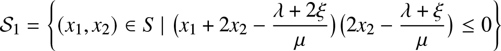 \begin{equation*} {{\mathcal{S}}}_1=
\left\{(x_1,x_2)\in S\;|\;\bigl(x_1+2x_2-\frac{\lambda +2\xi}{\mu}\bigr)\bigl(2x_2-\frac{\lambda+\xi}{\mu}\bigr)\leq 0\right\}
\end{equation*}
\begin{equation*} {{\mathcal{S}}}_1=
\left\{(x_1,x_2)\in S\;|\;\bigl(x_1+2x_2-\frac{\lambda +2\xi}{\mu}\bigr)\bigl(2x_2-\frac{\lambda+\xi}{\mu}\bigr)\leq 0\right\}
\end{equation*} \begin{equation*} {{\mathcal{S}}}_2=
\left\{(x_1,x_2)\in S\;|\;x_1+2x_2 \gt \frac{\lambda +2\xi}{\mu}\;,\;\frac{\lambda+\xi}{\mu} \lt 2x_2\right\}
\end{equation*}
\begin{equation*} {{\mathcal{S}}}_2=
\left\{(x_1,x_2)\in S\;|\;x_1+2x_2 \gt \frac{\lambda +2\xi}{\mu}\;,\;\frac{\lambda+\xi}{\mu} \lt 2x_2\right\}
\end{equation*} \begin{equation*} {{\mathcal{S}}}_3=
\left\{(x_1,x_2)\in S\;|\;x_1+2x_2 \lt \frac{\lambda +2\xi}{\mu}\;,\;\frac{\lambda+\xi}{\mu} \gt 2x_2\right\}
\end{equation*}
\begin{equation*} {{\mathcal{S}}}_3=
\left\{(x_1,x_2)\in S\;|\;x_1+2x_2 \lt \frac{\lambda +2\xi}{\mu}\;,\;\frac{\lambda+\xi}{\mu} \gt 2x_2\right\}
\end{equation*}See (4) for the explicit solution to the reflected ODE obtained above. This dynamical system admits a unique equilibrium point
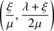 \begin{equation*}
\left(\frac{\xi}{\mu},\frac{\lambda+\xi}{2\mu}\right)
\end{equation*}
\begin{equation*}
\left(\frac{\xi}{\mu},\frac{\lambda+\xi}{2\mu}\right)
\end{equation*} Thus, according to the position of this equilibrium point in the convex set  ${\mathcal{S}}$, three possible regimes can be considered. Let
 \begin{equation*}
\rho \stackrel{def}{=} \frac{\lambda+ 2 \xi}{\mu}\end{equation*}
\begin{equation*}
\rho \stackrel{def}{=} \frac{\lambda+ 2 \xi}{\mu}\end{equation*} The under-loaded regime ( $\rho \lt {\bar{\beta}}$), the critically loaded regime ( $\rho = {\bar{\beta}}$) and the overloaded regime ( $\rho \gt {\bar{\beta}}$). Each of the aforementioned regimes will be developed in detail in the next sections.
4. The under-loaded regime
Throughout this section, we assume that the condition
 \begin{equation}
\rho \lt {\bar{\beta}}
\end{equation}
\begin{equation}
\rho \lt {\bar{\beta}}
\end{equation}holds.
In the Under-loaded regime, the equilibrium point ρ is less than  ${\bar{\beta}}$, and the figure below, fig. 2, illustrates the stabilization of the process $({\overline{X}}_1(t), {\overline{X}}_2(t))$ at the equilibrium point and never reaches the boundary $(\partial{\mathcal{S}})_2$.
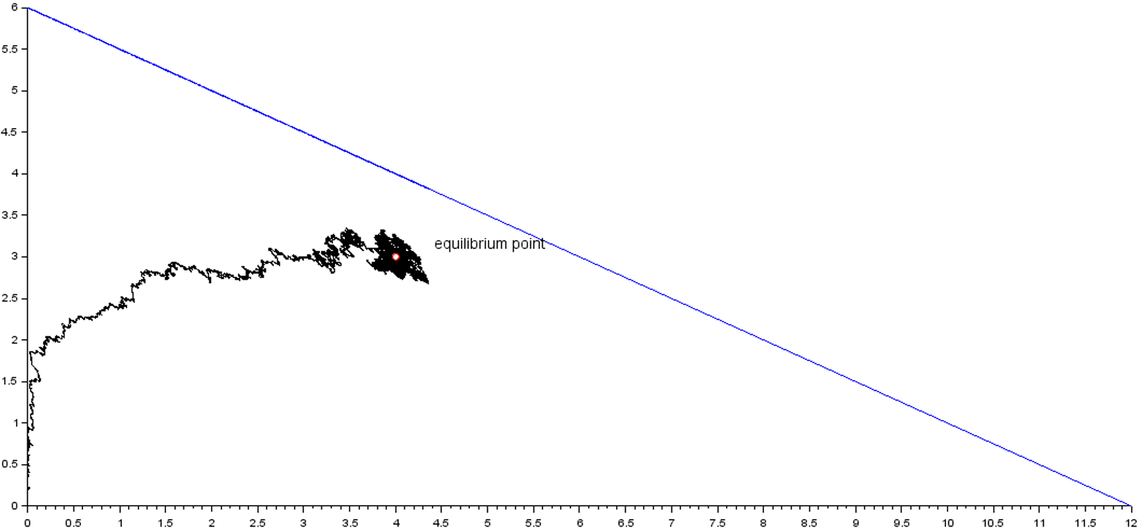
Figure 2. Simulation of the process  $({\overline{X}}_1(t), {\overline{X}}_2(t))$ with respect to the boundary $(\partial{\mathcal{S}})_2$
Let  $(X_1^N(t))$ and $(X_2^N(t))$ the processes given, respectively, by equations (7) and (8). Recall that $(X_1^N(t)+X_2^N(t))$ is the process describing the total number of files that are present in the system at time t. Let $(Z^N(t))$ be the process given by
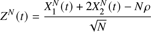 \begin{equation}
Z^N(t)=\dfrac{X_1^N(t)+2X_2^N(t)-N\rho}{\sqrt{N}}
\end{equation}
\begin{equation}
Z^N(t)=\dfrac{X_1^N(t)+2X_2^N(t)-N\rho}{\sqrt{N}}
\end{equation} The Q-matrix  $Q^{N} = (q^{N}(.,.))$ of the Markov process $ (X_1^N(t) ,X_2^N(t) ,Z^N(t)) $ is defined by;
For  $(x_1,x_2)\in{\mathcal{D}}^N$ and $z=\dfrac{x_1+2x_2-N\rho}{\sqrt{N}}$
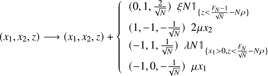 \begin{equation} (x_1,x_2,z) \longrightarrow (x_1,x_2,z)+
\left\{ \begin{array}{ll}
(0,1,\frac{2}{\sqrt{N}}) \ \ \xi N \mathbb{1}_{\lbrace z \lt \frac{{F}_{N} -1}{\sqrt{N}}-N\rho \rbrace} \\
(1,-1,-\frac{1}{\sqrt{N}})\ \ 2 \mu x_2\\
(-1,1,\frac{1}{\sqrt{N}}) \ \ \lambda N \mathbb{1}_{\lbrace x_1 \gt 0, z \lt \frac{{F}_{N}}{\sqrt{N}}-N\rho \rbrace}\\
(-1,0,-\frac{1}{\sqrt{N}}) \ \ \mu x_1
\end{array}
\right.
\end{equation}
\begin{equation} (x_1,x_2,z) \longrightarrow (x_1,x_2,z)+
\left\{ \begin{array}{ll}
(0,1,\frac{2}{\sqrt{N}}) \ \ \xi N \mathbb{1}_{\lbrace z \lt \frac{{F}_{N} -1}{\sqrt{N}}-N\rho \rbrace} \\
(1,-1,-\frac{1}{\sqrt{N}})\ \ 2 \mu x_2\\
(-1,1,\frac{1}{\sqrt{N}}) \ \ \lambda N \mathbb{1}_{\lbrace x_1 \gt 0, z \lt \frac{{F}_{N}}{\sqrt{N}}-N\rho \rbrace}\\
(-1,0,-\frac{1}{\sqrt{N}}) \ \ \mu x_1
\end{array}
\right.
\end{equation} and the generator of  $ (X_1^N(t) ,X_2^N(t) ,Z^N(t)) $ is given by,
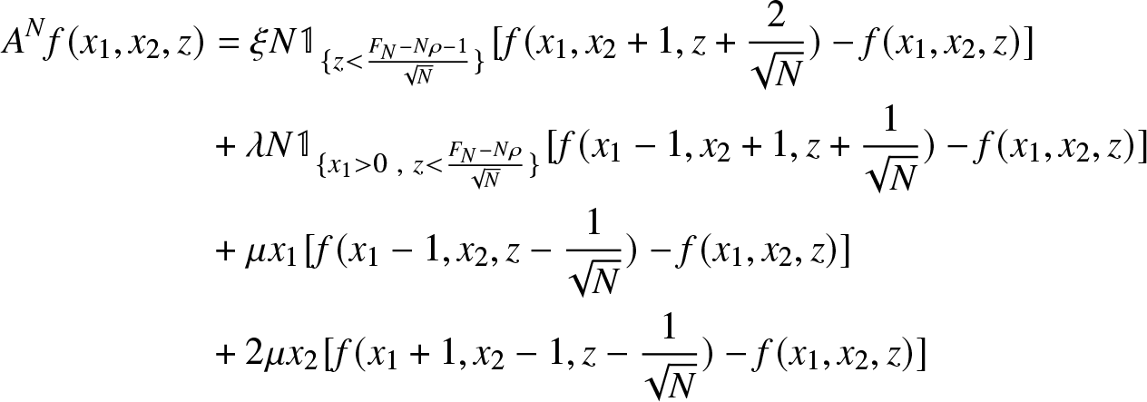 \begin{align*}
A^N f(x_1, x_2, z) & = \xi N \mathbb{1}_{\lbrace z \lt \frac{{F}_{N} - N \rho - 1}{\sqrt{N}} \rbrace} [f(x_1 , x_2 +1, z+ \frac{2}{\sqrt{N}}) - f(x_1, x_2, z)] \\
&+ \lambda N \mathbb{1}_{\lbrace x_1 \gt 0 \ , \ z \lt \frac{{F}_{N} - N \rho}{\sqrt{N}} \rbrace} [f(x_1 - 1, x_2 + 1, z+ \frac{1}{\sqrt{N}})- f(x_1, x_2, z)] \\
& + \mu x_1 [f(x_1 - 1, x_2, z- \frac{1}{\sqrt{N}}) - f(x_1, x_2, z)] \\
&+ 2 \mu x_2 [f(x_1 + 1, x_2 - 1, z- \frac{1} {\sqrt{N}}) - f(x_1, x_2, z)]
\end{align*}
\begin{align*}
A^N f(x_1, x_2, z) & = \xi N \mathbb{1}_{\lbrace z \lt \frac{{F}_{N} - N \rho - 1}{\sqrt{N}} \rbrace} [f(x_1 , x_2 +1, z+ \frac{2}{\sqrt{N}}) - f(x_1, x_2, z)] \\
&+ \lambda N \mathbb{1}_{\lbrace x_1 \gt 0 \ , \ z \lt \frac{{F}_{N} - N \rho}{\sqrt{N}} \rbrace} [f(x_1 - 1, x_2 + 1, z+ \frac{1}{\sqrt{N}})- f(x_1, x_2, z)] \\
& + \mu x_1 [f(x_1 - 1, x_2, z- \frac{1}{\sqrt{N}}) - f(x_1, x_2, z)] \\
&+ 2 \mu x_2 [f(x_1 + 1, x_2 - 1, z- \frac{1} {\sqrt{N}}) - f(x_1, x_2, z)]
\end{align*}For any function f depending only on the third variable z, i.e.,
 \begin{equation*}
f(x_1,x_2,z)=g(z)\quad \forall\;(x_1,x_2)\in\mathbb{N}^2 \quad with \quad x_1 \gt 0
\end{equation*}
\begin{equation*}
f(x_1,x_2,z)=g(z)\quad \forall\;(x_1,x_2)\in\mathbb{N}^2 \quad with \quad x_1 \gt 0
\end{equation*} for some twice differentiable function g on  $\mathbb{R}$ one gets
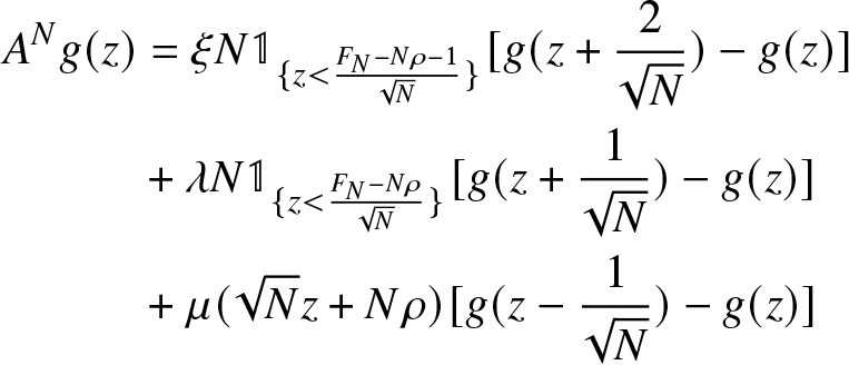 \begin{align*}
\nonumber
A^N g( z) & = \xi N \mathbb{1}_{\lbrace z \lt \frac{{F}_{N} - N \rho - 1}{\sqrt{N}} \rbrace} [g( z+ \frac{2}{\sqrt{N}}) - g( z)] \\
\nonumber
&+ \lambda N \mathbb{1}_{\lbrace z \lt \frac{{F}_{N} - N \rho}{\sqrt{N}} \rbrace} [g( z+ \frac{1}{\sqrt{N}})- g( z)] \\
\nonumber & + \mu(\sqrt{N}z+N\rho)[g(z- \frac{1}{\sqrt{N}}) - g( z)]
\end{align*}
\begin{align*}
\nonumber
A^N g( z) & = \xi N \mathbb{1}_{\lbrace z \lt \frac{{F}_{N} - N \rho - 1}{\sqrt{N}} \rbrace} [g( z+ \frac{2}{\sqrt{N}}) - g( z)] \\
\nonumber
&+ \lambda N \mathbb{1}_{\lbrace z \lt \frac{{F}_{N} - N \rho}{\sqrt{N}} \rbrace} [g( z+ \frac{1}{\sqrt{N}})- g( z)] \\
\nonumber & + \mu(\sqrt{N}z+N\rho)[g(z- \frac{1}{\sqrt{N}}) - g( z)]
\end{align*} Remark that condition (35) implies that terms  $\frac{{F}_{N} - N \rho - 1}{\sqrt{N}}$ and $\frac{{F}_{N} - N \rho}{\sqrt{N}}$ converge to $+\infty$. Thus the generator converges to
 \begin{equation*}
-\mu zg'(z)+(\lambda+3\xi)g''(z)\qquad z\in\mathbb{R}
\end{equation*}
\begin{equation*}
-\mu zg'(z)+(\lambda+3\xi)g''(z)\qquad z\in\mathbb{R}
\end{equation*} when  $N\rightarrow +\infty$, which is the generator of an Ornstein–Uhlenbeck process with variance converges to $\frac{\lambda+3\xi}{\mu}$. By results given in Ethier and Kurtz [Reference Ethier and Kurtz2] one can see that for some positive constant α the process $(X_1^N(t)+2X_2^N(t))$ lives in $[N\rho-\alpha N, N\rho+\alpha N]\subset [0,N{\bar{\beta}}]$ and the probability of saturation of the system is therefore small. In the under-loaded regime one can suppose that the capacity of the system is infinite, i.e., ${F}_{N}=+\infty$. In this case, the complete study of the process $(X_1^N(t),X_2^N(t))$ is made in the article El Kharroubi and El Masmari [Reference Kharroubi and Masmari7].
5. The overloaded regime
Throughout this section, we assume that the condition
 \begin{equation}
\rho \gt {\bar{\beta}}
\end{equation}
\begin{equation}
\rho \gt {\bar{\beta}}
\end{equation}holds.
In the Overloaded regime, the equilibrium point ρ exceeds  $ {\bar{\beta}} $, and the figure below, fig. 3, illustrates that the process $ ({\overline{X}}_1(t), {\overline{X}}_2(t)) $ being constrained by the boundary $ (\partial{\mathcal{S}})_2 $ and never reaching the equilibrium point.
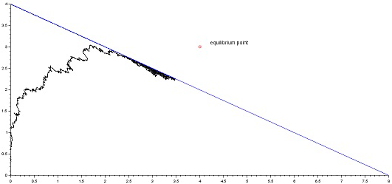
Figure 3. Simulation of the process  $({\overline{X}}_1(t), {\overline{X}}_2(t))$ with respect to the boundary $(\partial{\mathcal{S}})_2$
the Q-matrix  $Q^{N} = (q^{N}(.,.))$ and the generator of the Markov process $ ({X_1}^{N}(t/N), {X_2}^{N}(t/N) ,m^N(t/N)) $ are given by,
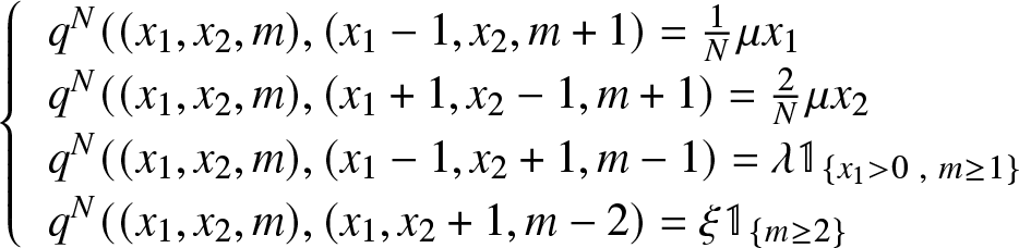 \begin{equation*}
\nonumber
\left\{ \begin{array}{ll}
q^{N}((x_1,x_2, m),(x_1 - 1, x_2, m+1)= \frac{1}{N} \mu x_1\\
q^{N}((x_1,x_2, m),(x_1 +1, x_2-1, m+ 1)= \frac{2}{N} \mu x_2 \\
q^{N}((x_1,x_2, m),(x_1 -1, x_2 + 1, m- 1)= \lambda \mathbb{1}_{\lbrace x_1 \gt 0 \ , \ m\geq 1 \rbrace} \\
q^{N}((x_1,x_2, m),(x_1 , x_2 +1, m- 2)= \xi \mathbb{1}_{\lbrace m\geq 2 \rbrace} \end{array}
\right.
\end{equation*}
\begin{equation*}
\nonumber
\left\{ \begin{array}{ll}
q^{N}((x_1,x_2, m),(x_1 - 1, x_2, m+1)= \frac{1}{N} \mu x_1\\
q^{N}((x_1,x_2, m),(x_1 +1, x_2-1, m+ 1)= \frac{2}{N} \mu x_2 \\
q^{N}((x_1,x_2, m),(x_1 -1, x_2 + 1, m- 1)= \lambda \mathbb{1}_{\lbrace x_1 \gt 0 \ , \ m\geq 1 \rbrace} \\
q^{N}((x_1,x_2, m),(x_1 , x_2 +1, m- 2)= \xi \mathbb{1}_{\lbrace m\geq 2 \rbrace} \end{array}
\right.
\end{equation*}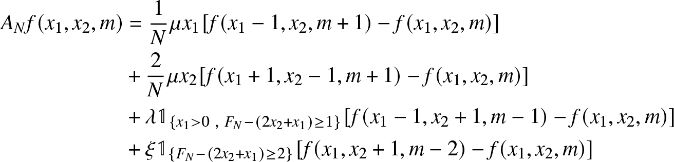 \begin{align*}
A_N f(x_1, x_2, m) & = \frac{1}{N} \mu x_1 [f(x_1 - 1, x_2, m+1) - f(x_1, x_2, m)] \\ &+ \frac{2}{N} \mu x_2 [f(x_1 +1, x_2-1, m+ 1)- f(x_1, x_2, m)] \\
& + \lambda \mathbb{1}_{\lbrace x_1 \gt 0 \ , \ {F}_{N} - (2 x_2 + x_1) \geq 1 \rbrace} [f(x_1 -1, x_2 + 1, m- 1) - f(x_1, x_2, m)] \\
&+ \xi \mathbb{1}_{\lbrace {F}_{N} - (2 x_2 + x_1) \geq 2 \rbrace} [f(x_1 , x_2 +1, m- 2) - f(x_1, x_2, m)]
\end{align*}
\begin{align*}
A_N f(x_1, x_2, m) & = \frac{1}{N} \mu x_1 [f(x_1 - 1, x_2, m+1) - f(x_1, x_2, m)] \\ &+ \frac{2}{N} \mu x_2 [f(x_1 +1, x_2-1, m+ 1)- f(x_1, x_2, m)] \\
& + \lambda \mathbb{1}_{\lbrace x_1 \gt 0 \ , \ {F}_{N} - (2 x_2 + x_1) \geq 1 \rbrace} [f(x_1 -1, x_2 + 1, m- 1) - f(x_1, x_2, m)] \\
&+ \xi \mathbb{1}_{\lbrace {F}_{N} - (2 x_2 + x_1) \geq 2 \rbrace} [f(x_1 , x_2 +1, m- 2) - f(x_1, x_2, m)]
\end{align*}For any function f depending only on the third variable m, i.e.,
 \begin{equation*}
f(x_1,x_2,m)=g(m)\quad \forall\;(x_1,x_2)\in\mathbb{N}^2
\end{equation*}
\begin{equation*}
f(x_1,x_2,m)=g(m)\quad \forall\;(x_1,x_2)\in\mathbb{N}^2
\end{equation*} for some function g on  $\mathbb{N}$ one gets
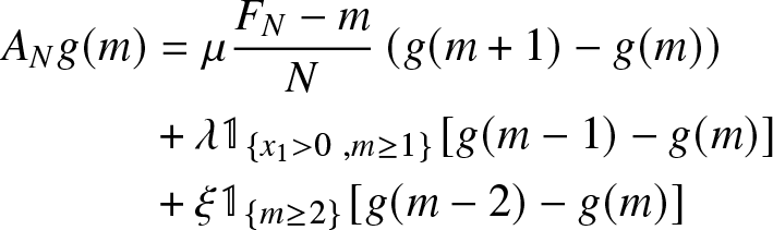 \begin{equation*}\begin{aligned}\nonumber
A_N g( m) & = \mu\frac{{F}_{N}-m}{N}\left(g(m+1) - g(m)\right) \\ \nonumber
&+ \lambda \mathbb{1}_{\lbrace x_1 \gt 0 \ , m \geq 1 \rbrace} [g( m- 1) - g(m)] \\ \nonumber
&+ \xi \mathbb{1}_{\lbrace m \geq 2 \rbrace} [g(m- 2) - g( m)]
\end{aligned}
\end{equation*}
\begin{equation*}\begin{aligned}\nonumber
A_N g( m) & = \mu\frac{{F}_{N}-m}{N}\left(g(m+1) - g(m)\right) \\ \nonumber
&+ \lambda \mathbb{1}_{\lbrace x_1 \gt 0 \ , m \geq 1 \rbrace} [g( m- 1) - g(m)] \\ \nonumber
&+ \xi \mathbb{1}_{\lbrace m \geq 2 \rbrace} [g(m- 2) - g( m)]
\end{aligned}
\end{equation*}This generator converges to
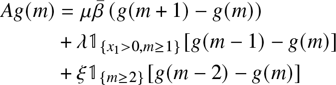 \begin{equation*}\begin{aligned}\nonumber
Ag( m) & = \mu{\bar{\beta}}\left(g(m+1) - g(m)\right) \\ \nonumber
&+ \lambda \mathbb{1}_{\lbrace x_1 \gt 0, m \geq 1 \rbrace} [g( m- 1) - g(m)] \\ \nonumber
&+ \xi \mathbb{1}_{\lbrace m \geq 2 \rbrace} [g(m- 2) - g( m)]
\end{aligned}
\end{equation*}
\begin{equation*}\begin{aligned}\nonumber
Ag( m) & = \mu{\bar{\beta}}\left(g(m+1) - g(m)\right) \\ \nonumber
&+ \lambda \mathbb{1}_{\lbrace x_1 \gt 0, m \geq 1 \rbrace} [g( m- 1) - g(m)] \\ \nonumber
&+ \xi \mathbb{1}_{\lbrace m \geq 2 \rbrace} [g(m- 2) - g( m)]
\end{aligned}
\end{equation*} Thus, for any  $x=(x_1,x_2)\in\mathbb{N}^*\times\mathbb{N}$, this is the generator of the Markov process $(m(t))$ with transitions
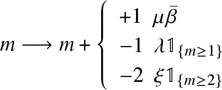 \begin{equation} m \longrightarrow m+
\left\{ \begin{array}{ll}
+1 \ \ \mu {\bar{\beta}} \\
-1 \ \ \lambda \mathbb{1}_{\{m \geq 1\}} \\
-2 \ \ \xi \mathbb{1}_{\{m \geq 2\}} \end{array}
\right.
\end{equation}
\begin{equation} m \longrightarrow m+
\left\{ \begin{array}{ll}
+1 \ \ \mu {\bar{\beta}} \\
-1 \ \ \lambda \mathbb{1}_{\{m \geq 1\}} \\
-2 \ \ \xi \mathbb{1}_{\{m \geq 2\}} \end{array}
\right.
\end{equation}Proposition 5.1. Under the condition (38), the process  $(m(t))$ has a unique invariant distribution π, its generating function $g(u) = {\underset{n \geq 0}{\sum }} \pi(n) u^n$ is given by, for $u\in[-1,1]$
 \begin{equation}
g(u) = \frac{1}{-\mu {\bar{\beta}}+ (\lambda+\xi) u +\xi} \left[(\lambda u+\xi (1+u)) \pi(0) +\xi (1+u) u \pi(1)\right]
\end{equation}
\begin{equation}
g(u) = \frac{1}{-\mu {\bar{\beta}}+ (\lambda+\xi) u +\xi} \left[(\lambda u+\xi (1+u)) \pi(0) +\xi (1+u) u \pi(1)\right]
\end{equation} Where  $( \pi(0), \pi(1))$ are given by
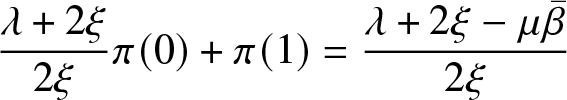
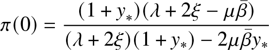 \begin{equation}
\pi(0) = \frac{({1+y}_{*}) (\lambda+2 \xi - \mu {\bar{\beta}})}{(\lambda+2\xi)( 1+y_{*}) -2\mu{\bar{\beta}}y_{*}}
\end{equation}
\begin{equation}
\pi(0) = \frac{({1+y}_{*}) (\lambda+2 \xi - \mu {\bar{\beta}})}{(\lambda+2\xi)( 1+y_{*}) -2\mu{\bar{\beta}}y_{*}}
\end{equation}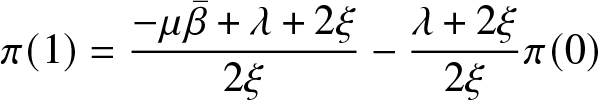 \begin{equation}
\pi(1)= \frac{-\mu {\bar{\beta}} + \lambda +2 \xi}{2 \xi} - \frac{\lambda + 2 \xi}{2 \xi } \pi(0)
\end{equation}
\begin{equation}
\pi(1)= \frac{-\mu {\bar{\beta}} + \lambda +2 \xi}{2 \xi} - \frac{\lambda + 2 \xi}{2 \xi } \pi(0)
\end{equation}with
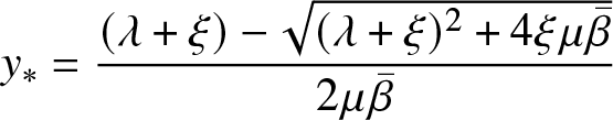 \begin{equation*}
y_{*} = \frac{(\lambda+\xi)- \sqrt{(\lambda+\xi)^2 + 4 \xi \mu {\bar{\beta}}}}{2 \mu {\bar{\beta}}}
\end{equation*}
\begin{equation*}
y_{*} = \frac{(\lambda+\xi)- \sqrt{(\lambda+\xi)^2 + 4 \xi \mu {\bar{\beta}}}}{2 \mu {\bar{\beta}}}
\end{equation*}Proof. The existence and uniqueness of the stationary distribution is a simple consequence of Foster’s criterion. See Proposition 8.14 of Robert [Reference Robert13]. For  $u \in [-1,1]$, define
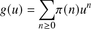 \begin{equation*}g(u) = {\underset{n \geq 0}{\sum }} \pi(n) u^n\end{equation*}
The equilibrium equation
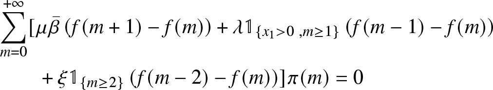 \begin{equation}
\begin{aligned}
&\sum_{m=0}^{+\infty}[\mu{\bar{\beta}}\left(f(m+1)-f(m)\right)+\lambda\mathbb{1}_{\lbrace x_1 \gt 0 \ , m \geq 1 \rbrace}\left(f(m-1)-f(m)\right)\\
&\qquad+\xi\mathbb{1}_{\lbrace m \geq 2 \rbrace}\left(f(m-2)-f(m)\right)] \pi(m)=0
\end{aligned}
\end{equation}
\begin{equation}
\begin{aligned}
&\sum_{m=0}^{+\infty}[\mu{\bar{\beta}}\left(f(m+1)-f(m)\right)+\lambda\mathbb{1}_{\lbrace x_1 \gt 0 \ , m \geq 1 \rbrace}\left(f(m-1)-f(m)\right)\\
&\qquad+\xi\mathbb{1}_{\lbrace m \geq 2 \rbrace}\left(f(m-2)-f(m)\right)] \pi(m)=0
\end{aligned}
\end{equation} for  $f(m)=u^m$, gives the following relation
 \begin{equation*}
g(u) (\mu {\bar{\beta}} u^2 (u-1) + \lambda (u-u^2) +\xi (1-u^2)) = \lambda (u-u^2) \pi(0) + \xi (1-u^2) ( \pi(0) + u \pi(1))
\end{equation*}
\begin{equation*}
g(u) (\mu {\bar{\beta}} u^2 (u-1) + \lambda (u-u^2) +\xi (1-u^2)) = \lambda (u-u^2) \pi(0) + \xi (1-u^2) ( \pi(0) + u \pi(1))
\end{equation*}Let
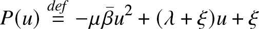 \begin{equation*}P(u)\stackrel{def}{=} - \mu {\bar{\beta}} u^2 +(\lambda +\xi) u +\xi \end{equation*}
then we have
 \begin{equation}
P(u) g(u) = ((\lambda+\xi) u+ \xi )\pi (0) + \xi (1+u) u \pi(1))
\end{equation}
\begin{equation}
P(u) g(u) = ((\lambda+\xi) u+ \xi )\pi (0) + \xi (1+u) u \pi(1))
\end{equation} Note that  $P(-1)=-( \mu {\bar{\beta}}+\lambda) \lt 0$, $P(0)=\xi$ and $P(1)=-\mu {\bar{\beta}}+\lambda+2\xi \gt 0$ by Condition (38). The function P(u) has a unique root in $[-1,1]$ and it is necessarily $y_*$.
We have therefore that  $y_*$ is a root of the RHS of the Relation (44), hence
 \begin{equation*}
\mu{\bar{\beta}}y_*^2\pi(0)+\xi y_*(1+y_*)\pi(1)=0
\end{equation*}
\begin{equation*}
\mu{\bar{\beta}}y_*^2\pi(0)+\xi y_*(1+y_*)\pi(1)=0
\end{equation*} and the relation  $g(1)=1$ gives the additional identity
 \begin{equation*}
\frac{\lambda+2\xi}{2 \xi} \pi(0)+\pi(1) =\frac{\lambda + 2 \xi - \mu {\bar{\beta}}}{2 \xi}
\end{equation*}
\begin{equation*}
\frac{\lambda+2\xi}{2 \xi} \pi(0)+\pi(1) =\frac{\lambda + 2 \xi - \mu {\bar{\beta}}}{2 \xi}
\end{equation*}The proposition is proved.
5.1. Fluid limits
Our aim in this section is to identify the limit of the renormalized processes  $({\bar{X}}_1^N(t))$ and $({\bar{X}}_2^N(t))$ given, respectively, by equations (18) and (19). We assume that
 \begin{equation}
\underset{N \rightarrow + \infty}{\text{lim}} \left( {\overline{X}}_1^N(0), {\overline{X}}_2^N(0) \right) = \left( x_1, x_2 \right)
\end{equation}
\begin{equation}
\underset{N \rightarrow + \infty}{\text{lim}} \left( {\overline{X}}_1^N(0), {\overline{X}}_2^N(0) \right) = \left( x_1, x_2 \right)
\end{equation} and we successively study the cases where  $(x_1,x_2)$ is chosen inside the set ${\mathcal{S}}$ and the case where $(x_1,x_2)$ lies on the boundary $(\partial {\mathcal{S}})_2$.
5.1.1. Starting from the interior of
$ {\mathcal{S}}$

Let  $T_1^N$ be the hitting time
 \begin{equation*}T_1^N=\inf\{t \gt 0\;|\; m^N(t)\in\{0,1\}\}\end{equation*}
 Note that before time  $T_1^N$ the Markov process $(X_1^N(t),X_2^N(t))$ coincides with the Markov process describing the storage process with infinite capacity ( ${F}_{N}=+\infty$).
The Proposition 5.4 proves the convergence in distribution of the hitting time  $T_1^N$. The proof of this result is inspired by the study of $M/M/N/N$ queue ( see Robert [Reference Robert13] and Fricker, Robert, and Tibi [Reference Fricker, Robert and Tibi4]). Let $\phi_c^N$ be the function on ${\mathbb{R}}^+$ defined by
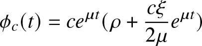 \begin{equation*}\phi_c(t) = ce^{\mu t} (\rho + \frac{c \xi }{2 \mu} e^{\mu t})\end{equation*}
 for  $c \in {\mathbb{R}}^*$, $N\in\mathbb{N}^*$.
Lemma 5.2. Let  $v=(1,2)$. The function
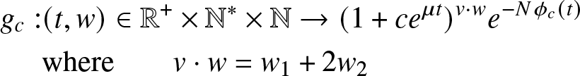 \begin{align*}
{g}_{c} : &(t,w) \in {\mathbb{R}}^+ \times \mathbb{N}^*\times\mathbb{N} \rightarrow (1+c e^{\mu t} )^ {v\cdot w} e^{- N\phi_c(t)}\\
&\text{where}\qquad v\cdot w=w_1+2w_2
\end{align*}
\begin{align*}
{g}_{c} : &(t,w) \in {\mathbb{R}}^+ \times \mathbb{N}^*\times\mathbb{N} \rightarrow (1+c e^{\mu t} )^ {v\cdot w} e^{- N\phi_c(t)}\\
&\text{where}\qquad v\cdot w=w_1+2w_2
\end{align*} is space-time harmonic with respect to the Q-matrix Q given in (4) with  ${F}_{N}=+\infty$. In other words
 \begin{equation*}\frac{\partial {g}_{c}}{\partial t} (t,w) + Q ({g}_{c}) (t,w) =0,\; \text{for all} \ t \in {\mathbb{R}}^+ \; \text{and for all} \; w \in \mathbb{N}^*\times\mathbb{N}\end{equation*}
Proof. For  $t\in{\mathbb{R}}_+$ and $w\in\mathbb{N}^*\times\mathbb{N}$
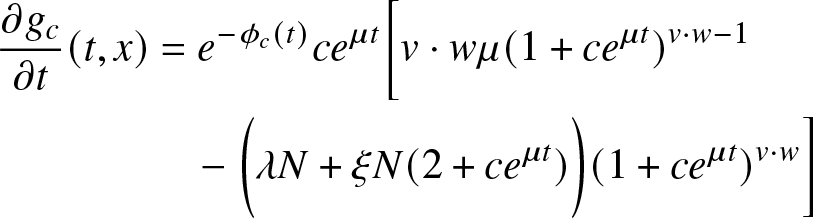 \begin{equation*}\nonumber
\begin{aligned}
\frac{\partial {g}_{c}}{\partial t} (t,x) & =e^{- \phi_c (t)}ce^{\mu t} \biggl[ v\cdot w \mu(1+c e^{\mu t})^ {v\cdot w-1}\\
& \quad- \biggl( \lambda N + \xi N(2+ c e^{\mu t})\biggr) (1+c e^{\mu t})^{v\cdot w}\biggr]
\end{aligned}
\end{equation*}
\begin{equation*}\nonumber
\begin{aligned}
\frac{\partial {g}_{c}}{\partial t} (t,x) & =e^{- \phi_c (t)}ce^{\mu t} \biggl[ v\cdot w \mu(1+c e^{\mu t})^ {v\cdot w-1}\\
& \quad- \biggl( \lambda N + \xi N(2+ c e^{\mu t})\biggr) (1+c e^{\mu t})^{v\cdot w}\biggr]
\end{aligned}
\end{equation*}on other hand
 \begin{equation*}Q({g}_{c})(t,w)=Q({g}_{c}(t,.))(w)\end{equation*}
is given by
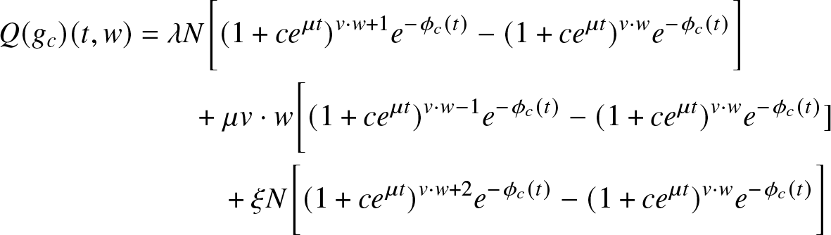 \begin{equation*}\nonumber
\begin{aligned}
Q({g}_{c})(t,w)& =\lambda N \biggl[(1+c e^{\mu t})^{v\cdot w+1} e^{- \phi_c (t)} - (1+c e^{\mu t})^{v\cdot w} e^{- \phi_c (t)}\biggr] \\
&\qquad + \mu {v\cdot w} \biggl[(1+c e^{\mu t})^{v\cdot w-1} e^{- \phi_c (t)} - (1+c e^{\mu t})^{v\cdot w} e^{- \phi_c (t)}]\\
& \quad\quad\quad+ \xi N \biggl[(1+c e^{\mu t})^{v\cdot w+2} e^{- \phi_c (t)} - (1+c e^{\mu t})^{v\cdot w}e^{- \phi_c (t)}\biggr]
\end{aligned}
\end{equation*}
\begin{equation*}\nonumber
\begin{aligned}
Q({g}_{c})(t,w)& =\lambda N \biggl[(1+c e^{\mu t})^{v\cdot w+1} e^{- \phi_c (t)} - (1+c e^{\mu t})^{v\cdot w} e^{- \phi_c (t)}\biggr] \\
&\qquad + \mu {v\cdot w} \biggl[(1+c e^{\mu t})^{v\cdot w-1} e^{- \phi_c (t)} - (1+c e^{\mu t})^{v\cdot w} e^{- \phi_c (t)}]\\
& \quad\quad\quad+ \xi N \biggl[(1+c e^{\mu t})^{v\cdot w+2} e^{- \phi_c (t)} - (1+c e^{\mu t})^{v\cdot w}e^{- \phi_c (t)}\biggr]
\end{aligned}
\end{equation*}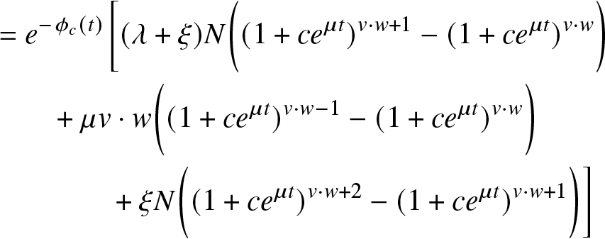 \begin{equation*}\nonumber
\begin{aligned}
& = e^{- \phi_c (t)} \biggl[(\lambda + \xi) N \biggl((1+c e^{\mu t})^{v\cdot w+1} - (1+c e^{\mu t})^{v\cdot w} \biggr)\\
&\qquad +\mu{v\cdot w} \biggl((1+c e^{\mu t})^{v\cdot w-1} - (1+c e^{\mu t})^{v\cdot w}\biggr )\\
& \qquad\qquad+ \xi N \biggl((1+c e^{\mu t})^{v\cdot w+2} -(1+c e^{\mu t})^{v\cdot w+1}\biggr )\biggr]
\end{aligned}
\end{equation*}
\begin{equation*}\nonumber
\begin{aligned}
& = e^{- \phi_c (t)} \biggl[(\lambda + \xi) N \biggl((1+c e^{\mu t})^{v\cdot w+1} - (1+c e^{\mu t})^{v\cdot w} \biggr)\\
&\qquad +\mu{v\cdot w} \biggl((1+c e^{\mu t})^{v\cdot w-1} - (1+c e^{\mu t})^{v\cdot w}\biggr )\\
& \qquad\qquad+ \xi N \biggl((1+c e^{\mu t})^{v\cdot w+2} -(1+c e^{\mu t})^{v\cdot w+1}\biggr )\biggr]
\end{aligned}
\end{equation*}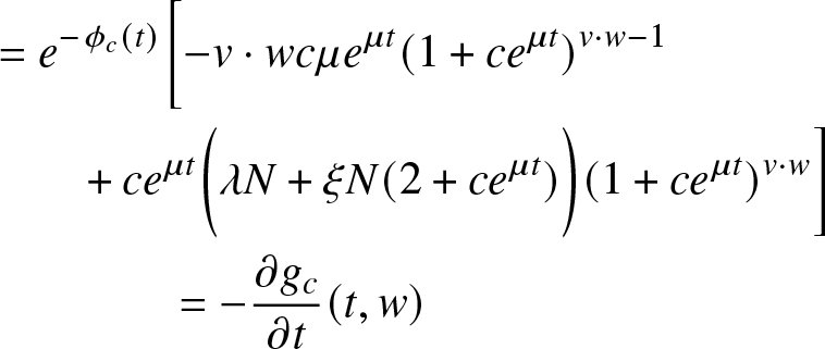 \begin{equation*}\nonumber
\begin{aligned}
& = e^{- \phi_c (t)} \biggl[- {v\cdot w}c \mu e^{\mu t} (1+c e^{\mu t})^{v\cdot w-1} \\
&\qquad +c e^{\mu t} \biggl(\lambda N + \xi N (2 + c e^{\mu t})\biggr) (1+c e^{\mu t})^{v\cdot w} \biggr]\\
&\qquad\qquad = - \frac{\partial {g}_{c}}{\partial t} (t,w)
\end{aligned}
\end{equation*}
\begin{equation*}\nonumber
\begin{aligned}
& = e^{- \phi_c (t)} \biggl[- {v\cdot w}c \mu e^{\mu t} (1+c e^{\mu t})^{v\cdot w-1} \\
&\qquad +c e^{\mu t} \biggl(\lambda N + \xi N (2 + c e^{\mu t})\biggr) (1+c e^{\mu t})^{v\cdot w} \biggr]\\
&\qquad\qquad = - \frac{\partial {g}_{c}}{\partial t} (t,w)
\end{aligned}
\end{equation*}(1) For
$c \in {\mathbb{R}}^*$ and
$N\in\mathbb{N}^*$ the process
(46)\begin{equation} \left( {g}_{c}(t,{X}^N(t))\right)
\end{equation}is a martingale.
(2) For
$N\in\mathbb{N}^*$ the following processes are martingales.
(47)\begin{equation}\left(e^{\mu t} (v\cdot {X}^N(t) - N\rho )\right)
\end{equation}(48)\begin{equation} \left( e^{2 \mu t} \left((v\cdot {X}^N(t) - N\rho )^2 - v\cdot {X}^N(t) - N\frac{\xi}{\mu}\right)\right)
\end{equation}


(1) By Lemma 5.2 the function
$(t,w)\rightarrow {g}_{c}(t,w)$ is space-time harmonic for the Q-matrix Q given in ((4)) with
${F}_{N}=+\infty$. Since
$t \rightarrow \frac{\partial {g}_{c}}{\partial t}$ is continuous, then the process
$({g}_{c}(t,{X}^N(t))$ is a local martingale (See Corollary B.5 in Robert [Reference Robert13]). Furthermore, for
$t \in {\mathbb{R}}^+$,
\begin{eqnarray*}
\nonumber v\cdot {X}^N(t) \leq (2 X_2^N(0) + X_1^N(0))+ 2 {\mathcal{N}}_{\xi_N}(]0,t]) + {\mathcal{N}}_{\lambda_N}(]0,t])
\end{eqnarray*}one gets for
$t\geq 0$,
\begin{equation*}\mathbb{E} ( \sup_{0 \leq s \leq t }|{g}_{c}(t,{X}^N(t)|) \lt + \infty\end{equation*}Thus the process
$({g}_{c}(t,{X}^N(t))$ is a martingale (see proposition A.7 in Robert [Reference Robert13]).(2) Let Ψ be the function on
${\mathbb{R}}^+\times \mathbb{N}$ defined by
\begin{equation*}\Psi(x,z)=(1+x)^ze^{-N\rho x}e^{-\frac{N\xi}{2\mu}x^2}\end{equation*}Note that
\begin{equation*}\Psi(ce^{\mu t},v\cdot {X}^N(t))={g}_{c}(t,{X}^N(t))\end{equation*}and therefore
$(\Psi(ce^{\mu t},v\cdot {X}^N(t))$ is a martingale. On other hand, it is well known that
\begin{equation*}e^{-N\rho x}(1+x)^z=\sum_{n\geq 0}C_n^{N\rho}(z)\frac{{x}^n}{n!}
\end{equation*}where
$C_n^{N\rho}(z)$ is the nth Poisson-Charlier polynomial (see Chihara [Reference Theodore16]). Hence, the expansion of
$\Psi(x,z)$ is given by(49)\begin{equation}
\Psi(x,z)=\sum_{n\geq 0}\left(\sum_{k=0}^nC_{n-k}^{N\rho}(z)b_k\right)\frac{{x}^n}{n!}
\end{equation}where
$b_{2k+1}=0$ and
$b_{2k}=\left(-\frac{N\xi}{2\mu}\right)^k$


Replacing in (49) x and z by  $ce^{\mu t}$ and $v\cdot {X}^N(t)$, respectively, one gets that for any $n\in\mathbb{N}^*$,
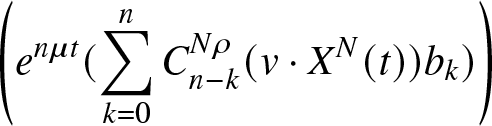 \begin{equation*}\left( e^{n\mu t}(\sum_{k=0}^nC_{n-k}^{N\rho}(v\cdot {X}^N(t))b_k)\right)\end{equation*}
is a martingale. In particular for n = 1 and n = 2 one gets that the processes
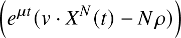 \begin{equation*}\left(e^{\mu t}(v\cdot {X}^N(t)-N\rho)\right)\end{equation*}
and
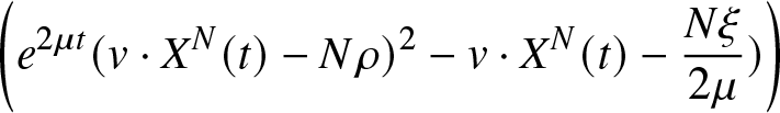 \begin{equation*}\left(e^{2\mu t}(v\cdot {X}^N(t)-N\rho)^2-v\cdot {X}^N(t)-\frac{N\xi}{2\mu})\right)\end{equation*}
are martingales.
Proposition 5.4. if Conditions (38) and (45) hold with  $x_1+2x_2 \lt {\bar{\beta}}$ then the hitting time $T_{1}^N$ converges in distribution to T 0 where
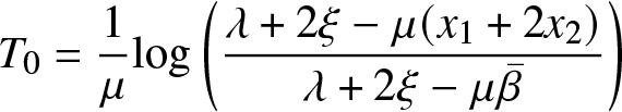 \begin{equation}
T_0 = \frac{1}{\mu} \text{log} \left( \frac{\lambda + 2 \xi - \mu (x_1 + 2 x_2)}{\lambda + 2 \xi - \mu {\bar{\beta}}} \right)
\end{equation}
\begin{equation}
T_0 = \frac{1}{\mu} \text{log} \left( \frac{\lambda + 2 \xi - \mu (x_1 + 2 x_2)}{\lambda + 2 \xi - \mu {\bar{\beta}}} \right)
\end{equation}Proof. We assume that Conditions (38) and (45) hold with  $x_1+2x_2 \lt {\bar{\beta}}$. Doob’s optional stopping Theorem applied to the martingale given in (47) and to $T_1^N$ show that the process
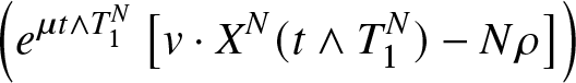 \begin{equation*} \nonumber
\left(e^{\mu t \wedge T_{1}^N}\left[ v\cdot {X}^{N}(t \wedge T_{1}^N)- N\rho \right]\right)
\end{equation*}
\begin{equation*} \nonumber
\left(e^{\mu t \wedge T_{1}^N}\left[ v\cdot {X}^{N}(t \wedge T_{1}^N)- N\rho \right]\right)
\end{equation*}is a martingale. Thus, the following equality holds
 \begin{equation*} \mathbb{E} \left(e^{\mu t \wedge T_{1}^N}\left[N\rho -v\cdot {X}^{N}(t \wedge T_{1}^N) \right]\right)= N\rho-v\cdot {X}^{N}(0)
\end{equation*}
\begin{equation*} \mathbb{E} \left(e^{\mu t \wedge T_{1}^N}\left[N\rho -v\cdot {X}^{N}(t \wedge T_{1}^N) \right]\right)= N\rho-v\cdot {X}^{N}(0)
\end{equation*} Since  $v\cdot {X}^{N} (t \wedge T_{1}^N) \leq {F}_{N}-1$, one gets that,
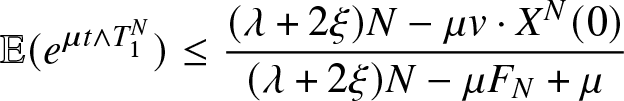 \begin{equation*} \nonumber \mathbb{E} (e^{\mu t \wedge T_{1}^N} ) \leq \frac{(\lambda + 2\xi) N - \mu v\cdot {X}^{N}(0)}{(\lambda + 2\xi) N - \mu {F}_{N}+\mu}
\end{equation*}
\begin{equation*} \nonumber \mathbb{E} (e^{\mu t \wedge T_{1}^N} ) \leq \frac{(\lambda + 2\xi) N - \mu v\cdot {X}^{N}(0)}{(\lambda + 2\xi) N - \mu {F}_{N}+\mu}
\end{equation*}By letting t go to infinity, monotone convergence Theorem shows that
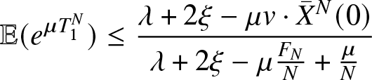 \begin{equation*} \nonumber \mathbb{E} (e^{\mu T_{1}^N} ) \leq \frac{\lambda + 2\xi - \mu v\cdot{\bar{X}}^N(0)}{\lambda + 2\xi - \mu \frac{{F}_{N}}{N}+\frac{\mu}{N}}
\end{equation*}
\begin{equation*} \nonumber \mathbb{E} (e^{\mu T_{1}^N} ) \leq \frac{\lambda + 2\xi - \mu v\cdot{\bar{X}}^N(0)}{\lambda + 2\xi - \mu \frac{{F}_{N}}{N}+\frac{\mu}{N}}
\end{equation*}And that implies uniform integrability of the martingale
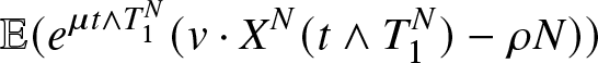 \begin{equation*} \nonumber \mathbb{E} (e^{\mu t \wedge T_{1}^N} (v\cdot {X}^{N} (t \wedge T_{1}^N)- \rho N))
\end{equation*}
\begin{equation*} \nonumber \mathbb{E} (e^{\mu t \wedge T_{1}^N} (v\cdot {X}^{N} (t \wedge T_{1}^N)- \rho N))
\end{equation*}One gets therefore the following identity
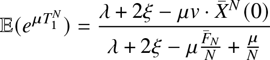 \begin{equation}\mathbb{E} (e^{\mu T_1^N}) = \frac{\lambda +2 \xi -\mu v\cdot{\bar{X}}^N(0)}{\lambda + 2 \xi - \mu \frac{{\bar{F}}_N}{N}+\frac{\mu}{N} }
\end{equation}
\begin{equation}\mathbb{E} (e^{\mu T_1^N}) = \frac{\lambda +2 \xi -\mu v\cdot{\bar{X}}^N(0)}{\lambda + 2 \xi - \mu \frac{{\bar{F}}_N}{N}+\frac{\mu}{N} }
\end{equation} Doob’s optional stopping theorem applied again to the martingale given by (48) and to the stopping time  $T_1^N$ shows that the process
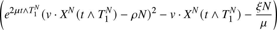 \begin{equation*} \nonumber \left(e^{{2 \mu t \wedge T_{1}^N}} (v\cdot {X}^{N}(t \wedge T_{1}^N)- \rho N)^{2} - v\cdot {X}^{N}(t\wedge T_{1}^N) - \frac{\xi N}{\mu}\right)
\end{equation*}
\begin{equation*} \nonumber \left(e^{{2 \mu t \wedge T_{1}^N}} (v\cdot {X}^{N}(t \wedge T_{1}^N)- \rho N)^{2} - v\cdot {X}^{N}(t\wedge T_{1}^N) - \frac{\xi N}{\mu}\right)
\end{equation*} is a martingale. Since  $v\cdot {X}^{N} (t \wedge T_{1}^N) \leq {F}_{N}-1$, $N{\bar{\beta}} \lt N\rho$ and $N{\bar{\beta}}= {F}_{N}$ one could then use the same arguments used above to get the following identity
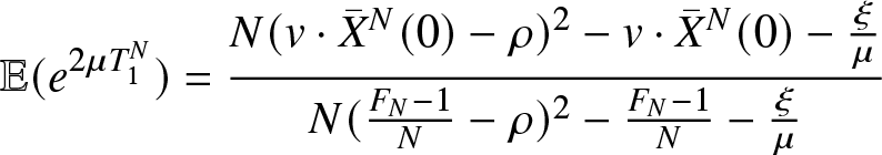 \begin{equation}\mathbb{E} (e^{{2 \mu T_{1}^N}}) = \frac{N (v\cdot{\bar{X}}^N(0)- \rho )^{2} - v\cdot{\bar{X}}^N(0) - \frac{\xi }{\mu}}{N(\frac{{F}_{N}-1}{N}- \rho)^{2} - \frac{{F}_{N}-1}{N} - \frac{\xi }{\mu}}
\end{equation}
\begin{equation}\mathbb{E} (e^{{2 \mu T_{1}^N}}) = \frac{N (v\cdot{\bar{X}}^N(0)- \rho )^{2} - v\cdot{\bar{X}}^N(0) - \frac{\xi }{\mu}}{N(\frac{{F}_{N}-1}{N}- \rho)^{2} - \frac{{F}_{N}-1}{N} - \frac{\xi }{\mu}}
\end{equation} One then deduces that  $var(e^{\mu T_{1}^N}) = O(1/N)$ and the Tchebychev inequality implies that, for ϵ > 0,
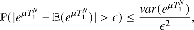 \begin{equation*}\mathbb{P} (| e^{\mu T_{1}^N} - \mathbb{E} (e^{\mu T_{1}^N} ) | \gt \epsilon) \leq \frac{var(e^{\mu T_{1}^N})}{\epsilon^{2}},\end{equation*}
 Hence, using the identity given by (51), the sequence  $(T_1^N)$ converges in probability to T 0.
Theorem 5.5 If Conditions (38) and (45) hold with  $x_1+2x_2 \lt {\bar{\beta}}$ and $x_2 \gt \frac{\lambda+\xi}{2\mu}$ Then for the convergence in distribution,
 \begin{equation*} \nonumber \underset{N \rightarrow + \infty}{lim} ({\overline{X}}_1^N(t),{\overline{X}}_2^N(t))_{0\leq t \leq T_0} =({\bar{x}}_1(t),{\bar{x}}_2(t))_{0\leq t \leq T_0}
\end{equation*}
\begin{equation*} \nonumber \underset{N \rightarrow + \infty}{lim} ({\overline{X}}_1^N(t),{\overline{X}}_2^N(t))_{0\leq t \leq T_0} =({\bar{x}}_1(t),{\bar{x}}_2(t))_{0\leq t \leq T_0}
\end{equation*} with  $({\bar{x}}_1(t), {\bar{x}}_2(t)) $ are given in (31).
Note that at time T 0 , the fluid limit  $({\bar{x}}_1(t), {\bar{x}}_2(t)) $ hits the boundary ${(\partial{\mathcal{S}})}_2$, i.e., ${\bar{x}}_1(T_0) + 2 {\bar{x}}_2(T_0) = {\bar{\beta}}$.
Proof. We assume that Conditions (38) and (45) hold with  $x_1+2x_2 \lt {\bar{\beta}}$ and $x_2 \gt \frac{\lambda+\xi}{2\mu}$. By Theorem 3.2 the sequence
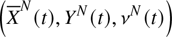 \begin{equation*}\left({\overline{X}}^{N}(t),Y^{N}(t), \nu^N(t)\right)\end{equation*}
 is relatively compact in  $\mathcal{D}({\mathbb{R}}_+,{\mathbb{R}}^3)$ and the limit $\left( x(.) ,y(.), \nu(.)\right)$ of any convergent subsequence satisfies for all $t\geq 0$:
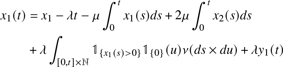 \begin{equation}
\begin{aligned}
x_1(t) &= x_1 - \lambda t-\mu \int_{0}^t x_1(s)ds + 2\mu \int_{0}^t x_2(s) ds \\
&+ \lambda \int_{[0,t] \times \mathbb{N}} \mathbb{1}_{\lbrace x_1(s) \gt 0 \rbrace} \mathbb{1}_{\lbrace 0 \rbrace} (u) \nu (ds \times du) +\lambda y_1(t)
\end{aligned}
\end{equation}
\begin{equation}
\begin{aligned}
x_1(t) &= x_1 - \lambda t-\mu \int_{0}^t x_1(s)ds + 2\mu \int_{0}^t x_2(s) ds \\
&+ \lambda \int_{[0,t] \times \mathbb{N}} \mathbb{1}_{\lbrace x_1(s) \gt 0 \rbrace} \mathbb{1}_{\lbrace 0 \rbrace} (u) \nu (ds \times du) +\lambda y_1(t)
\end{aligned}
\end{equation} \begin{equation}
\begin{aligned} x_2(t)
&= x_2 + (\lambda+\xi) t -2 \mu \int_{0}^t x_2(s) ds- \xi \nu ([0,t] \times \{0,1\}) \\ & - \lambda \int_{[0,t] \times \mathbb{N}} \mathbb{1}_{\lbrace x_1(s) \gt 0 \rbrace} \mathbb{1}_{\lbrace 0 \rbrace} (u) \nu (ds \times du) - \lambda y_1(t)
\end{aligned}
\end{equation}
\begin{equation}
\begin{aligned} x_2(t)
&= x_2 + (\lambda+\xi) t -2 \mu \int_{0}^t x_2(s) ds- \xi \nu ([0,t] \times \{0,1\}) \\ & - \lambda \int_{[0,t] \times \mathbb{N}} \mathbb{1}_{\lbrace x_1(s) \gt 0 \rbrace} \mathbb{1}_{\lbrace 0 \rbrace} (u) \nu (ds \times du) - \lambda y_1(t)
\end{aligned}
\end{equation} The condition  $x_2 \gt \frac{\lambda+\xi}{2\mu}$ implies that the function $y_1(t)=0$ for all $t\geq 0$ (see Theorem 2 in El Kharroubi and El Masmari [Reference Kharroubi and Masmari7]). Thus, it is sufficient to show that for all $t\leq T_0$
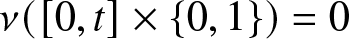 \begin{equation*}\nu ([0,t] \times \{0,1\})=0\end{equation*}
Let us first recall that,
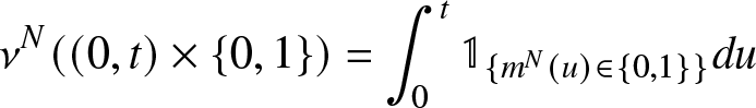 \begin{equation*} \nu^N((0,t)\times \{0,1\})=\int_0^t\mathbb{1}_{\{m^N(u)\in\{0,1\}\}}du\end{equation*}
 and that the increasing sequence of hitting times  $(T_1^N)$ converges in probability to T 0. For any $t\leq T_0$ and for any ϵ > 0
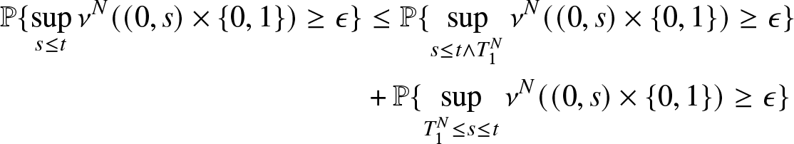 \begin{align*}
\mathbb{P}\{\sup_{s\leq t}\nu^N((0,s)\times \{0,1\})\geq\epsilon\}&\leq
\mathbb{P}\{\sup_{s\leq t\wedge T_1^N }\nu^N((0,s)\times \{0,1\})\geq\epsilon\}\\
\qquad &+ \mathbb{P}\{\sup_{T_1^N\leq s\leq t }\nu^N((0,s)\times \{0,1\})\geq\epsilon\}
\end{align*}
\begin{align*}
\mathbb{P}\{\sup_{s\leq t}\nu^N((0,s)\times \{0,1\})\geq\epsilon\}&\leq
\mathbb{P}\{\sup_{s\leq t\wedge T_1^N }\nu^N((0,s)\times \{0,1\})\geq\epsilon\}\\
\qquad &+ \mathbb{P}\{\sup_{T_1^N\leq s\leq t }\nu^N((0,s)\times \{0,1\})\geq\epsilon\}
\end{align*} The first term of the RHS of the above Inequality is equal to zero. Since for  $T_1^N\leq s\leq t $
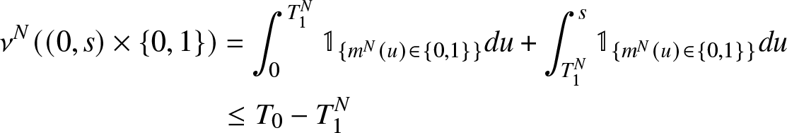 \begin{align*}
\nu^N((0,s)\times \{0,1\})&=\int_0^{T_1^N}\mathbb{1}_{\{m^N(u)\in\{0,1\}\}}du+\int_{T_1^N}^s\mathbb{1}_{\{m^N(u)\in\{0,1\}\}}du\\
&\leq T_0-T_1^N
\end{align*}
\begin{align*}
\nu^N((0,s)\times \{0,1\})&=\int_0^{T_1^N}\mathbb{1}_{\{m^N(u)\in\{0,1\}\}}du+\int_{T_1^N}^s\mathbb{1}_{\{m^N(u)\in\{0,1\}\}}du\\
&\leq T_0-T_1^N
\end{align*} \begin{equation*}\mathbb{P}\{\sup_{s\leq t}\nu^N((0,s)\times \{0,1\})\geq\epsilon\}\leq
\mathbb{P}\{|T^N-T_0|\geq\epsilon\} \end{equation*}
\begin{equation*}\mathbb{P}\{\sup_{s\leq t}\nu^N((0,s)\times \{0,1\})\geq\epsilon\}\leq
\mathbb{P}\{|T^N-T_0|\geq\epsilon\} \end{equation*}Thus,
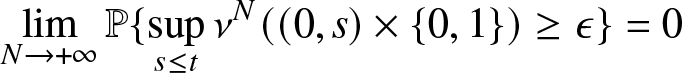 \begin{equation*}\lim_{N\rightarrow +\infty}\mathbb{P}\{\sup_{s\leq t}\nu^N((0,s)\times \{0,1\})\geq\epsilon\}=0\end{equation*}
 Application 1 : In that case, simulations have shown that if one assumes that if the system starts from the interior of the domain  $ {\mathcal{S}}$, $ x_1 + 2x_2 \lt {\bar{\beta}}$, the storage system before $ T_1^N$ behaves like the system with infinite capacity, and the processes $( X_{0}^N(t))$, $( X_{1}^N(t))$ and $( X_{2}^N(t))$ in the finite capacity case are close to the processes $( X_{0}^N(t))$, $( X_{1}^N(t))$ and $( X_{2}^N(t))$ without constraints on the boundary ${F}_{N}$. And the better choice of parameters that guarantees reliability remains the same as in the infinite capacity case before T 1,
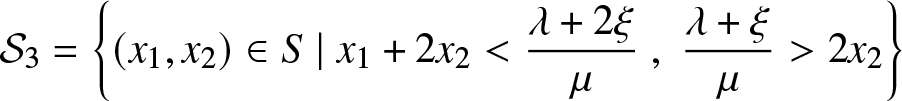 \begin{equation*} {{\mathcal{S}}}_3=
\left\{(x_1,x_2)\in S\;|\;x_1+2x_2 \lt \frac{\lambda +2\xi}{\mu}\;,\;\frac{\lambda+\xi}{\mu} \gt 2x_2\right\}
\end{equation*}
\begin{equation*} {{\mathcal{S}}}_3=
\left\{(x_1,x_2)\in S\;|\;x_1+2x_2 \lt \frac{\lambda +2\xi}{\mu}\;,\;\frac{\lambda+\xi}{\mu} \gt 2x_2\right\}
\end{equation*}The graphs below illustrate the closeness of the processes with finite capacity, represented by the color red, and those with infinite capacity, represented by the color blue in figs. 4a), 4b and 4c)
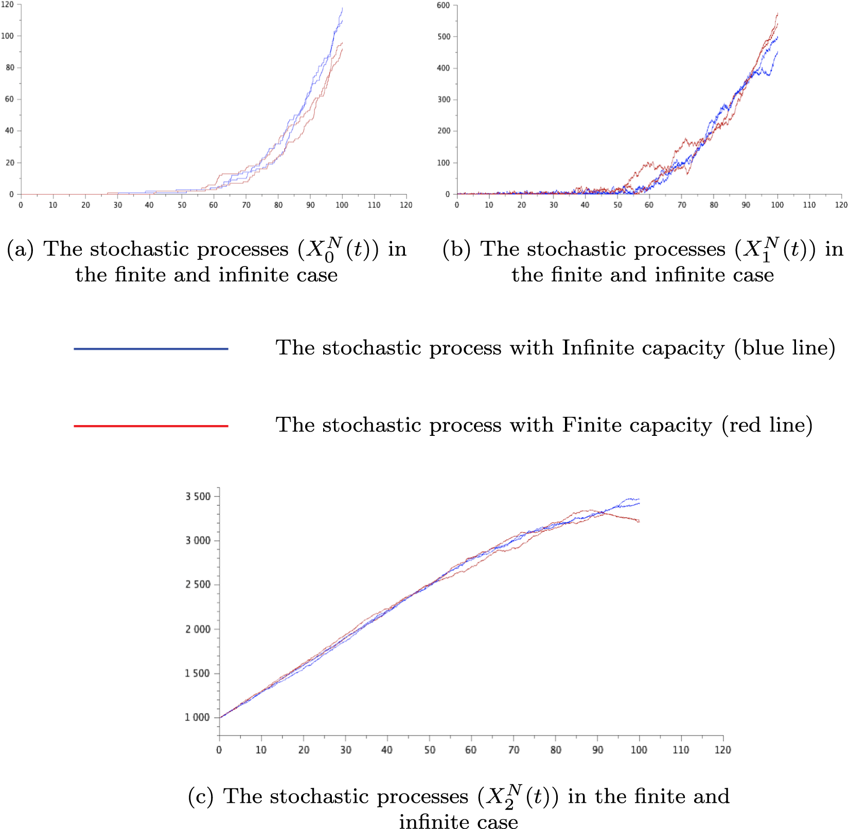
Figure 4. Comparison between the stochastic processes in the finite and infinite case before  $T_{1}^N$. a) The stochastic processes $( X_{0}^N(t))$ in the finite and infinite case. b) The stochastic processes $( X_{1}^N(t))$ in the finite and infinite case. c) The stochastic processes $( X_{2}^N(t))$ in the finite and infinite case.
5.1.2. Starting from the boundary of
$(\partial{\mathcal{S}})_2$ of the set
${\mathcal{S}}$


Theorem 5.6 If Conditions (38) and (45) hold with  $x_1+2x_2={\bar{\beta}}$. Then for the convergence in distribution,
 \begin{equation*} \underset{N \rightarrow + \infty}{lim} ({\bar{X}}_1^N(t),{\bar{X}}_2^N(t))_{t \geq 0} = (x_1(t), x_2(t))_{t \geq 0}
\end{equation*}
\begin{equation*} \underset{N \rightarrow + \infty}{lim} ({\bar{X}}_1^N(t),{\bar{X}}_2^N(t))_{t \geq 0} = (x_1(t), x_2(t))_{t \geq 0}
\end{equation*} where  $(x_1(t), x_2(t))_{t \geq 0} $ is the solution of the ordinary differential equation,
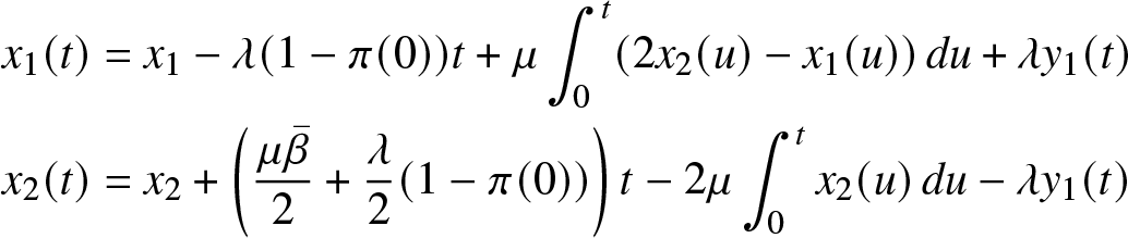 \begin{equation}
\begin{aligned}
x_1(t) &= x_1 - \lambda (1-\pi(0))t + \mu \int_{0}^t (2 x_2(u) - x_1(u)) \, du + \lambda y_1(t) \\
x_2(t) &= x_2 + \left(\frac{\mu{\bar{\beta}}}{2}+\frac{\lambda}{2}(1-\pi(0))\right) t -2 \mu \int_{0}^t x_2(u) \, du - \lambda y_1(t)
\end{aligned}
\end{equation}
\begin{equation}
\begin{aligned}
x_1(t) &= x_1 - \lambda (1-\pi(0))t + \mu \int_{0}^t (2 x_2(u) - x_1(u)) \, du + \lambda y_1(t) \\
x_2(t) &= x_2 + \left(\frac{\mu{\bar{\beta}}}{2}+\frac{\lambda}{2}(1-\pi(0))\right) t -2 \mu \int_{0}^t x_2(u) \, du - \lambda y_1(t)
\end{aligned}
\end{equation} where  $\pi(0)$ is defined by Equation (41).
Proof. Our goal is to identify the measure ν in Equations (53) and (54). The Q-matrix of the Markov process  $({X}^N(.), m^N(.))$ is given by,
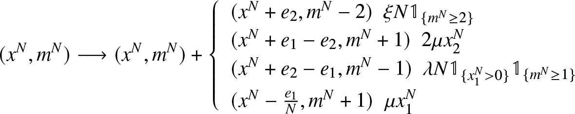 \begin{equation*}\nonumber (x^N,m^N) \longrightarrow (x^N,m^N)+
\left\{ \begin{array}{ll}
(x^N+e_2,m^N-2) \ \ \xi N \mathbb{1}_{\{m^N \geq 2\}} \\
(x^N+e_1-e_2,m^N+1)\ \ 2 \mu x_2^N\\
(x^N+e_2-e_1,m^N-1) \ \ \lambda N \mathbb{1}_{\{x_1^N \gt 0\}} \mathbb{1}_{\{m^N \geq 1\}} \\
(x^N-\frac{{e}_1}{N},m^N+1) \ \ \mu x_1^N
\end{array}
\right.
\end{equation*}
\begin{equation*}\nonumber (x^N,m^N) \longrightarrow (x^N,m^N)+
\left\{ \begin{array}{ll}
(x^N+e_2,m^N-2) \ \ \xi N \mathbb{1}_{\{m^N \geq 2\}} \\
(x^N+e_1-e_2,m^N+1)\ \ 2 \mu x_2^N\\
(x^N+e_2-e_1,m^N-1) \ \ \lambda N \mathbb{1}_{\{x_1^N \gt 0\}} \mathbb{1}_{\{m^N \geq 1\}} \\
(x^N-\frac{{e}_1}{N},m^N+1) \ \ \mu x_1^N
\end{array}
\right.
\end{equation*}Thus, the process
 \begin{equation*}\left(f({X}^N(t), m^N(t) ) - f({X}^N(0), m^N(0) )-\int_0^t (Qf)({X}^N(s), m^N(s) )ds\right)
\end{equation*}
\begin{equation*}\left(f({X}^N(t), m^N(t) ) - f({X}^N(0), m^N(0) )-\int_0^t (Qf)({X}^N(s), m^N(s) )ds\right)
\end{equation*} is a martingale for all bounded function f on  ${\mathbb{R}}^+\times \bar{\mathbb{N}}$. In particular the process
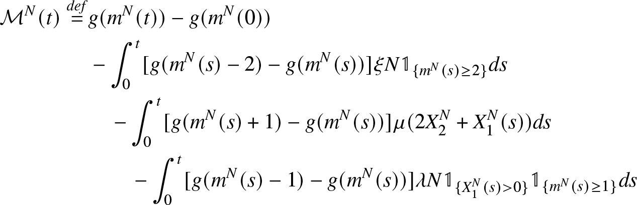 \begin{equation}
\begin{aligned}
\mathcal{M}^N(t)\stackrel{def}{=}&g(m^N(t)) - g(m^N(0))\\
& - \int_{0}^t [g(m^N(s)-2)- g(m^N(s))]\xi N \mathbb{1}_{\{m^N(s) \geq 2\}}ds \\
&\quad -\int_{0}^t [g(m^N(s)+1) - g(m^N(s))] \mu(2X_2^N+X_1^N(s))ds \\
&\qquad -\int_{0}^t [g(m^N(s)-1) - g(m^N(s))] \lambda N \mathbb{1}_{\{X_1^N(s) \gt 0\}} \mathbb{1}_{\{m^N(s) \geq 1\}}ds
\end{aligned}
\end{equation}
\begin{equation}
\begin{aligned}
\mathcal{M}^N(t)\stackrel{def}{=}&g(m^N(t)) - g(m^N(0))\\
& - \int_{0}^t [g(m^N(s)-2)- g(m^N(s))]\xi N \mathbb{1}_{\{m^N(s) \geq 2\}}ds \\
&\quad -\int_{0}^t [g(m^N(s)+1) - g(m^N(s))] \mu(2X_2^N+X_1^N(s))ds \\
&\qquad -\int_{0}^t [g(m^N(s)-1) - g(m^N(s))] \lambda N \mathbb{1}_{\{X_1^N(s) \gt 0\}} \mathbb{1}_{\{m^N(s) \geq 1\}}ds
\end{aligned}
\end{equation} is a martingale for all bounded function g on  $\bar{\mathbb{N}}$. It follows from Doob’s inequality that the process $ (\frac{\mathcal{M}^N(t)}{N})$ converges in distribution to 0.
Since  $2{\bar{X}}_2^N(t)+{\bar{X}}_1^N(t)=\frac{{F}_{N}}{N}-\frac{m^N(t)}{N}$, Equation (56) can be rewritten as
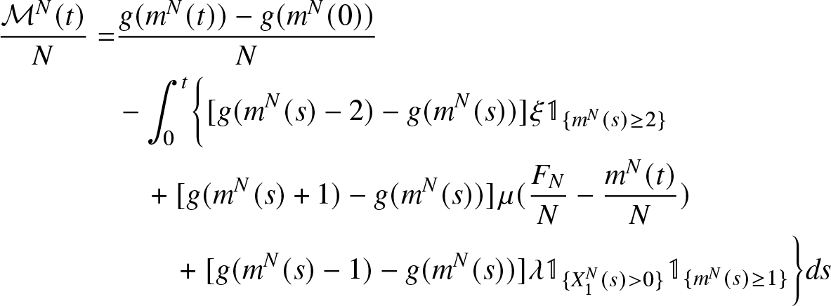 \begin{equation}
\begin{aligned}
\frac{{\mathcal{M}}^N(t)}{N}=&\frac{g(m^N(t)) - g(m^N(0))}{N}\\
& - \int_{0}^t\biggl\{[g(m^N(s)-2)- g(m^N(s))]\xi \mathbb{1}_{\{m^N(s) \geq 2\}} \\
&\quad + [g(m^N(s)+1) - g(m^N(s))] \mu(\frac{{F}_{N}}{N}-\frac{m^N(t)}{N}) \\
&\qquad + [g(m^N(s)-1) - g(m^N(s))] \lambda \mathbb{1}_{\{X_1^N(s) \gt 0\}} \mathbb{1}_{\{m^N(s) \geq 1\}}\biggr\} ds
\end{aligned}
\end{equation}
\begin{equation}
\begin{aligned}
\frac{{\mathcal{M}}^N(t)}{N}=&\frac{g(m^N(t)) - g(m^N(0))}{N}\\
& - \int_{0}^t\biggl\{[g(m^N(s)-2)- g(m^N(s))]\xi \mathbb{1}_{\{m^N(s) \geq 2\}} \\
&\quad + [g(m^N(s)+1) - g(m^N(s))] \mu(\frac{{F}_{N}}{N}-\frac{m^N(t)}{N}) \\
&\qquad + [g(m^N(s)-1) - g(m^N(s))] \lambda \mathbb{1}_{\{X_1^N(s) \gt 0\}} \mathbb{1}_{\{m^N(s) \geq 1\}}\biggr\} ds
\end{aligned}
\end{equation} In terms of measure  $\nu^N(.)$, we may rewrite the last term on the RHS of (57) as follows :
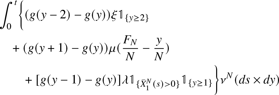 \begin{equation}
\begin{aligned}
& \int_{0}^t\biggl\{(g(y-2)- g(y))\xi \mathbb{1}_{\{y \geq 2\}}\\
&\quad + (g(y+1) - g(y)) \mu(\frac{{F}_{N}}{N}-\frac{y}{N})\\
&\qquad + [g(y-1) - g(y)] \lambda \mathbb{1}_{\{{\bar{X}}_1^N(s) \gt 0\}} \mathbb{1}_{\{y \geq 1\}}\biggr\}\nu^N(ds\times dy)
\end{aligned}
\end{equation}
\begin{equation}
\begin{aligned}
& \int_{0}^t\biggl\{(g(y-2)- g(y))\xi \mathbb{1}_{\{y \geq 2\}}\\
&\quad + (g(y+1) - g(y)) \mu(\frac{{F}_{N}}{N}-\frac{y}{N})\\
&\qquad + [g(y-1) - g(y)] \lambda \mathbb{1}_{\{{\bar{X}}_1^N(s) \gt 0\}} \mathbb{1}_{\{y \geq 1\}}\biggr\}\nu^N(ds\times dy)
\end{aligned}
\end{equation} which also converges to 0 since  $\frac{1}{N}\left(g(m^N(t)) - g(m^N(0))\right)$ converges to 0 as $N\rightarrow+\infty$. Furthermore, by continuous mapping theorem one gets that
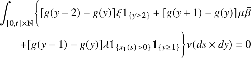 \begin{equation*}\begin{aligned}\nonumber \int_{[0,t]\times \mathbb{N}} \biggl\{[g(y-2)- g(y)] \xi \mathbb{1}_{\{y \geq 2\}} + [g(y+1) - g(y)] \mu {\bar{\beta}} \\ \nonumber
+ [g(y-1) - g(y)] \lambda \mathbb{1}_{\{x_1(s) \gt 0\}} \mathbb{1}_{\{y \geq 1\}} \biggr\} \nu(ds \times dy) =0
\end{aligned}
\end{equation*}
\begin{equation*}\begin{aligned}\nonumber \int_{[0,t]\times \mathbb{N}} \biggl\{[g(y-2)- g(y)] \xi \mathbb{1}_{\{y \geq 2\}} + [g(y+1) - g(y)] \mu {\bar{\beta}} \\ \nonumber
+ [g(y-1) - g(y)] \lambda \mathbb{1}_{\{x_1(s) \gt 0\}} \mathbb{1}_{\{y \geq 1\}} \biggr\} \nu(ds \times dy) =0
\end{aligned}
\end{equation*} for all  $t\geq 0$.
Thus, for almost all  $t \geq 0$,
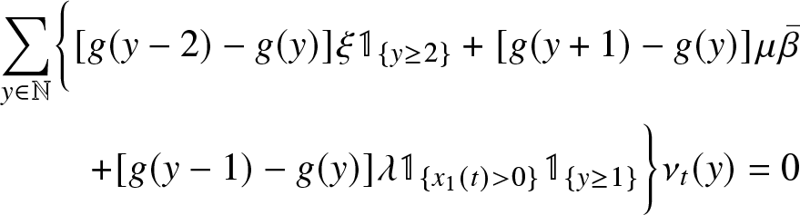 \begin{equation*}\begin{aligned}\nonumber \sum_{y\in \mathbb{N}} \biggl\{[g(y-2)- g(y)] \xi \mathbb{1}_{\{y \geq 2\}} + [g(y+1) - g(y)] \mu {\bar{\beta}} \\ \nonumber
+ [g(y-1) - g(y)] \lambda \mathbb{1}_{\{x_1(t) \gt 0\}} \mathbb{1}_{\{y \geq 1\}} \biggr\}\nu_t (y) =0
\end{aligned}
\end{equation*}
\begin{equation*}\begin{aligned}\nonumber \sum_{y\in \mathbb{N}} \biggl\{[g(y-2)- g(y)] \xi \mathbb{1}_{\{y \geq 2\}} + [g(y+1) - g(y)] \mu {\bar{\beta}} \\ \nonumber
+ [g(y-1) - g(y)] \lambda \mathbb{1}_{\{x_1(t) \gt 0\}} \mathbb{1}_{\{y \geq 1\}} \biggr\}\nu_t (y) =0
\end{aligned}
\end{equation*} Hence, for all  $t\geq 0$ such that $x_1(t) \gt 0$, the measure $\nu_t(.)=\pi$ where the measure π is invariant for the Markov process $(m(t))$ with Q-matrix given by (39). The theorem is proved.
Application 2: In the Overloaded case, if the system starts from the boundary  $\partial {{\mathcal{S}}}_2$, i.e., $x_1 + 2 x_2 = {\bar{\beta}}$, and the parameters have been fixed as follows:
- The number of nodes N = 100,
- The duplication rate is
$\lambda = 0,3$,- The admitting rate is ξ = 0.3,
- The loss rate is µ = 0.01,
- The maximal number of files to be stored in the system is
$F_{max} = 7000$.


In the simulations below, it will be shown that the fluid limits  $(x_0(t), x_1(t),x_2(t))$ obtained in (55) coincide with the stochastic process $(X_0^N(t), X_1^N(t),X_2^N(t))$ defined for the model. And the new coming files for storage are accepted with approximately the rate $\xi N (1 - \pi_{{\bar{\beta}}}(0))$. On the other hand, the reliability of the system is not impacted by the capacity of the system in this case.
See the graphs below, fig. 5 which clearly illustrate the striking alignment between the stochastic processes and their corresponding fluid limits. This strong correspondence underscores the critical role of the fluid limits in accurately capturing and describing the asymptotic behavior of the stochastic processes.
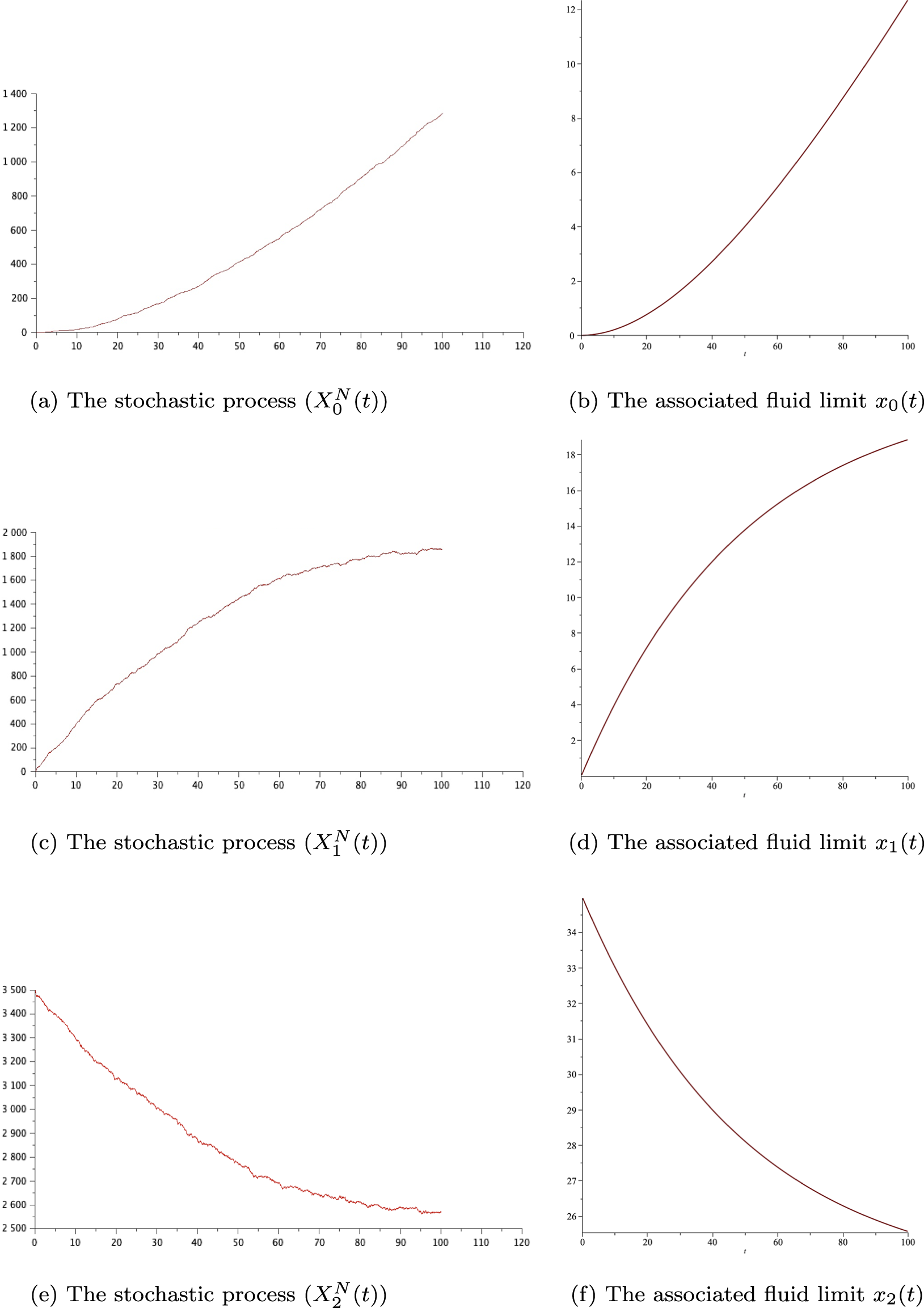
Figure 5. Comparison between the stochastic processes  $X_0^N(t), X_1^N(t), X_2^N(t)$ and their respective fluid limits $x_0(t), x_1(t), x_2(t)$. a) The stochastic process $ (X_0^N(t))$. b) The associated fluid limit $ x_0(t)$. c) The stochastic process $ (X_1^N(t))$. d) The associated fluid limit $ x_1(t)$. e) The stochastic process $ (X_2^N(t))$. f) The associated fluid limit $ x_2(t)$.
6. The critically loaded regime
In the Critically-loaded regime, the equilibrium point ρ is identical to  $ {\bar{\beta}} $, and the figure below, fig. 6, illustrates that the process $ ({\overline{X}}_1(t), {\overline{X}}_2(t)) $ being constrained by the boundary $ (\partial{\mathcal{S}})_2 $ which coincides with the equilibrium point.
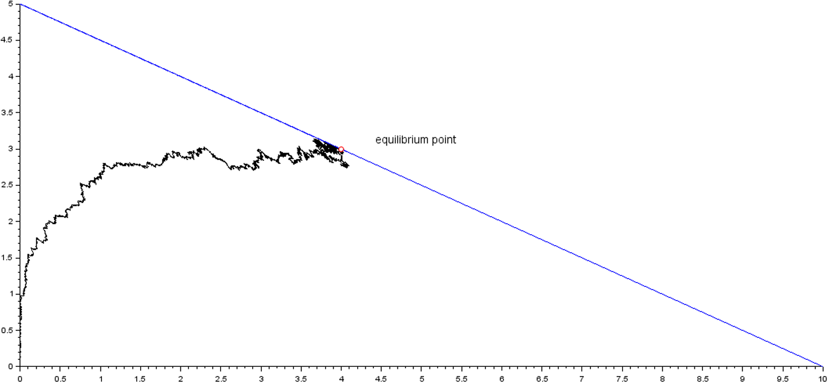
Figure 6. The equilibrium point in the critically loaded regime
Throughout this section, we assume that the condition
 \begin{equation}
\rho={\bar{\beta}}
\end{equation}
\begin{equation}
\rho={\bar{\beta}}
\end{equation} holds. Let  $\lbrace Z_1^N(t),Z_2^N(t),Z^N(t)\rbrace$ be the Markov process defined by
 \begin{equation*}Z_1^N(t)=\sqrt{N}(\rho_1-{\bar{X}}_1^N(t)),\quad Z_2^N(t)=\sqrt{N}(\rho_2-{\bar{X}}_2^N(t))\end{equation*}
and
 \begin{equation*}Z^N(t)=\sqrt{N}(\rho-{\bar{X}}_1^N(t)-2{\bar{X}}_2^N(t))=Z_1^N(t)+2Z_2^N(t)\end{equation*}
where
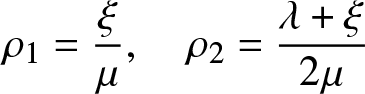 \begin{equation*}\rho_1=\frac{\xi}{\mu},\quad \rho_2=\frac{\lambda+\xi}{2\mu}\end{equation*}
In the following proposition we prove that the sequence of processes
 \begin{equation*}\lbrace Z_1^N(t),Z_2^N(t),Z^N(t)\rbrace\end{equation*}
converges in distribution to a reflected three-dimensional Ornstein–Uhlenbeck process.
The Q-matrix  $Q^{N} = (q^{N}(.,.))$ and the generator of the Markov process $\lbrace Z_1^N(t),Z_2^N(t),Z^N(t)\rbrace$
are given by:
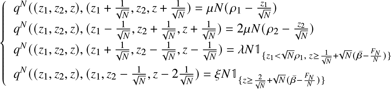 \begin{equation*}
\nonumber
\left\{ \begin{array}{ll}
q^{N}((z_1,z_2, z),(z_1+\frac{1}{\sqrt{N}}, z_2, z+\frac{1}{\sqrt{N}})=\mu N(\rho_1-\frac{z_1}{\sqrt{N}})\\
q^{N}((z_1,z_2, z),(z_1-\frac{1}{\sqrt{N}}, z_2+\frac{1}{\sqrt{N}}, z+\frac{1}{\sqrt{N}})= 2\mu N(\rho_2-\frac{z_2}{\sqrt{N}} ) \\
q^{N}((z_1,z_2, z),(z_1+\frac{1}{\sqrt{N}}, z_2-\frac{1}{\sqrt{N}}, z-\frac{1}{\sqrt{N}})= \lambda N \mathbb{1}_{\lbrace z_1 \lt \sqrt{N}\rho_1,\;z\geq \frac{1}{\sqrt{N}}+\sqrt{N}({\bar{\beta}}-\frac{{F}_{N}}{N}) \rbrace} \\
q^{N}((z_1,z_2, z),(z_1, z_2-\frac{1}{\sqrt{N}}, z-2\frac{1}{\sqrt{N}})= \xi N \mathbb{1}_{\lbrace z\geq \frac{2}{\sqrt{N}}+\sqrt{N}({\bar{\beta}}-\frac{{F}_{N}}{N}) \rbrace} \end{array}
\right.
\end{equation*}
\begin{equation*}
\nonumber
\left\{ \begin{array}{ll}
q^{N}((z_1,z_2, z),(z_1+\frac{1}{\sqrt{N}}, z_2, z+\frac{1}{\sqrt{N}})=\mu N(\rho_1-\frac{z_1}{\sqrt{N}})\\
q^{N}((z_1,z_2, z),(z_1-\frac{1}{\sqrt{N}}, z_2+\frac{1}{\sqrt{N}}, z+\frac{1}{\sqrt{N}})= 2\mu N(\rho_2-\frac{z_2}{\sqrt{N}} ) \\
q^{N}((z_1,z_2, z),(z_1+\frac{1}{\sqrt{N}}, z_2-\frac{1}{\sqrt{N}}, z-\frac{1}{\sqrt{N}})= \lambda N \mathbb{1}_{\lbrace z_1 \lt \sqrt{N}\rho_1,\;z\geq \frac{1}{\sqrt{N}}+\sqrt{N}({\bar{\beta}}-\frac{{F}_{N}}{N}) \rbrace} \\
q^{N}((z_1,z_2, z),(z_1, z_2-\frac{1}{\sqrt{N}}, z-2\frac{1}{\sqrt{N}})= \xi N \mathbb{1}_{\lbrace z\geq \frac{2}{\sqrt{N}}+\sqrt{N}({\bar{\beta}}-\frac{{F}_{N}}{N}) \rbrace} \end{array}
\right.
\end{equation*}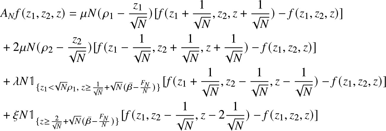 \begin{equation*}\begin{aligned}\nonumber
&A_N f(z_1, z_2, z) = \mu N(\rho_1-\frac{{z}_1}{\sqrt{N}}) [f(z_1+\frac{1}{\sqrt{N}}, z_2, z+\frac{1}{\sqrt{N}}) - f(z_1,z_2, z)] \\ \nonumber
&+ 2\mu N(\rho_2-\frac{{z}_2}{\sqrt{N}} ) [f(z_1-\frac{1}{\sqrt{N}}, z_2+\frac{1}{\sqrt{N}}, z+\frac{1}{\sqrt{N}})- f(z_1,z_2, z)] \\ \nonumber
& + \lambda N \mathbb{1}_{\lbrace z_1 \lt \sqrt{N}\rho_1,\;z\geq \frac{1}{\sqrt{N}}+\sqrt{N}({\bar{\beta}}-\frac{{F}_{N}}{N}) \rbrace} [f(z_1+\frac{1}{\sqrt{N}}, z_2-\frac{1}{\sqrt{N}}, z-\frac{1}{\sqrt{N}}) - f(z_1,z_2, z)] \\ \nonumber
&+ \xi N \mathbb{1}_{\lbrace z\geq \frac{2}{\sqrt{N}}+\sqrt{N}({\bar{\beta}}-\frac{{F}_{N}}{N}) \rbrace} [f(z_1, z_2-\frac{1}{\sqrt{N}}, z-2\frac{1}{\sqrt{N}}) - f(z_1,z_2, z)]
\end{aligned}
\end{equation*}
\begin{equation*}\begin{aligned}\nonumber
&A_N f(z_1, z_2, z) = \mu N(\rho_1-\frac{{z}_1}{\sqrt{N}}) [f(z_1+\frac{1}{\sqrt{N}}, z_2, z+\frac{1}{\sqrt{N}}) - f(z_1,z_2, z)] \\ \nonumber
&+ 2\mu N(\rho_2-\frac{{z}_2}{\sqrt{N}} ) [f(z_1-\frac{1}{\sqrt{N}}, z_2+\frac{1}{\sqrt{N}}, z+\frac{1}{\sqrt{N}})- f(z_1,z_2, z)] \\ \nonumber
& + \lambda N \mathbb{1}_{\lbrace z_1 \lt \sqrt{N}\rho_1,\;z\geq \frac{1}{\sqrt{N}}+\sqrt{N}({\bar{\beta}}-\frac{{F}_{N}}{N}) \rbrace} [f(z_1+\frac{1}{\sqrt{N}}, z_2-\frac{1}{\sqrt{N}}, z-\frac{1}{\sqrt{N}}) - f(z_1,z_2, z)] \\ \nonumber
&+ \xi N \mathbb{1}_{\lbrace z\geq \frac{2}{\sqrt{N}}+\sqrt{N}({\bar{\beta}}-\frac{{F}_{N}}{N}) \rbrace} [f(z_1, z_2-\frac{1}{\sqrt{N}}, z-2\frac{1}{\sqrt{N}}) - f(z_1,z_2, z)]
\end{aligned}
\end{equation*}Proposition 6.1. If f is twice differentiable on  ${\mathbb{R}}^3$ and such that $\nabla f(z_1,z_2,0)=0$ then the generator converges to
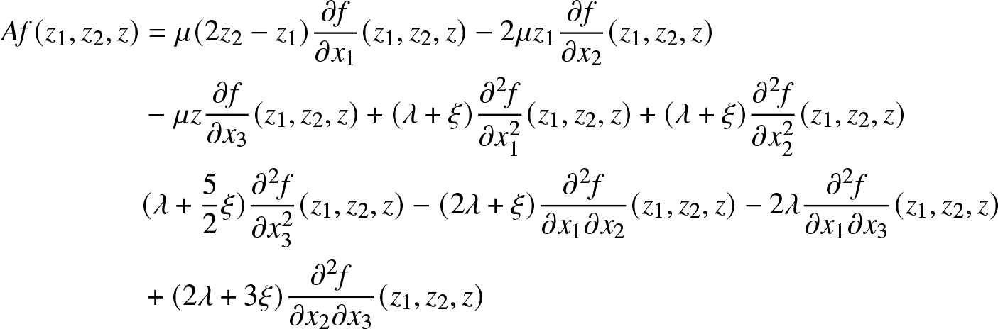 \begin{equation}
\begin{aligned}
Af(z_1,z_2,z)&=\mu (2z_2-z_1)\frac{\partial f}{\partial x_1}(z_1,z_2,z)-2\mu z_1\frac{\partial f}{\partial x_2}(z_1,z_2,z)\\
&-\mu z\frac{\partial f}{\partial {x}_{3}}(z_1,z_2,z)+(\lambda+\xi)\frac{{\partial}^2 f}{\partial x_1^2}(z_1,z_2,z)+(\lambda+\xi)\frac{{\partial}^2 f}{\partial x_2^2}(z_1,z_2,z)\\
&(\lambda+\frac{5}{2}\xi)\frac{{\partial}^2 f}{\partial {x}_{3}^2}(z_1,z_2,z)-(2\lambda+\xi)\frac{{\partial}^2 f}{\partial x_1\partial x_2}(z_1,z_2,z)-2\lambda\frac{{\partial}^2 f}{\partial x_1\partial {x}_{3}}(z_1,z_2,z)\\
&+(2\lambda+3\xi)\frac{{\partial}^2 f}{\partial x_2\partial {x}_{3}}(z_1,z_2,z)
\end{aligned}
\end{equation}
\begin{equation}
\begin{aligned}
Af(z_1,z_2,z)&=\mu (2z_2-z_1)\frac{\partial f}{\partial x_1}(z_1,z_2,z)-2\mu z_1\frac{\partial f}{\partial x_2}(z_1,z_2,z)\\
&-\mu z\frac{\partial f}{\partial {x}_{3}}(z_1,z_2,z)+(\lambda+\xi)\frac{{\partial}^2 f}{\partial x_1^2}(z_1,z_2,z)+(\lambda+\xi)\frac{{\partial}^2 f}{\partial x_2^2}(z_1,z_2,z)\\
&(\lambda+\frac{5}{2}\xi)\frac{{\partial}^2 f}{\partial {x}_{3}^2}(z_1,z_2,z)-(2\lambda+\xi)\frac{{\partial}^2 f}{\partial x_1\partial x_2}(z_1,z_2,z)-2\lambda\frac{{\partial}^2 f}{\partial x_1\partial {x}_{3}}(z_1,z_2,z)\\
&+(2\lambda+3\xi)\frac{{\partial}^2 f}{\partial x_2\partial {x}_{3}}(z_1,z_2,z)
\end{aligned}
\end{equation}for z > 0 and to
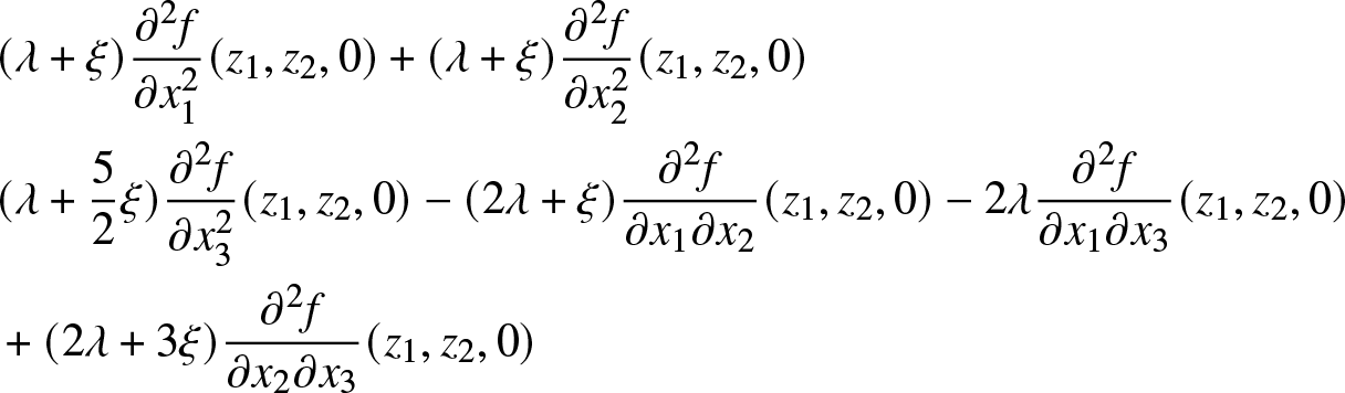 \begin{equation}
\begin{aligned}
&(\lambda+\xi)\frac{{\partial}^2 f}{\partial x_1^2}(z_1,z_2,0)+(\lambda+\xi)\frac{{\partial}^2 f}{\partial x_2^2}(z_1,z_2,0)\\
&(\lambda+\frac{5}{2}\xi)\frac{{\partial}^2 f}{\partial {x}_{3}^2}(z_1,z_2,0)-(2\lambda+\xi)\frac{{\partial}^2 f}{\partial x_1\partial x_2}(z_1,z_2,0)-2\lambda\frac{{\partial}^2 f}{\partial x_1\partial {x}_{3}}(z_1,z_2,0)\\
&+(2\lambda+3\xi)\frac{{\partial}^2 f}{\partial x_2\partial {x}_{3}}(z_1,z_2,0)
\end{aligned}
\end{equation}
\begin{equation}
\begin{aligned}
&(\lambda+\xi)\frac{{\partial}^2 f}{\partial x_1^2}(z_1,z_2,0)+(\lambda+\xi)\frac{{\partial}^2 f}{\partial x_2^2}(z_1,z_2,0)\\
&(\lambda+\frac{5}{2}\xi)\frac{{\partial}^2 f}{\partial {x}_{3}^2}(z_1,z_2,0)-(2\lambda+\xi)\frac{{\partial}^2 f}{\partial x_1\partial x_2}(z_1,z_2,0)-2\lambda\frac{{\partial}^2 f}{\partial x_1\partial {x}_{3}}(z_1,z_2,0)\\
&+(2\lambda+3\xi)\frac{{\partial}^2 f}{\partial x_2\partial {x}_{3}}(z_1,z_2,0)
\end{aligned}
\end{equation}which is the generator of the three-dimensional Ornstein–Uhlenbeck process reflected on the boundary of the half-space z > 0. One could refer to the following papers Ward and Glynn [Reference Ward and Glynn19], Ward and Glynn [Reference Ward and Glynn18], and Lidong and Chunmei [Reference Zhang and Jiang20] where the properties of the reflected Ornstein–Uhlenbeck and the associated infinitesimal generator are presented.
Acknowledgments
The authors are grateful to Philippe Robert for useful conversations and exchange of notes during the preparation of this work.
Competing interests
The authors declare none.


 Open access