


1. Introduction
Symmetrization procedures have a wide range of applications in modern analysis, geometric variational problems and optimization. Understanding the behaviour of functional and perimeter inequalities under symmetrization allows to prove the existence of symmetric minimisers of geometric variational problems, and to provide comparison principles for solutions of PDEs (see, for instance [Reference Cianchi and Fusco9, Reference Gidas, Ni and Nirenberg14, Reference Kawohl15, Reference Kawohl16, Reference Morgan and Pratelli19, Reference Pólya and Szegö21, Reference Serrin22, Reference Talenti24, Reference Trombetti, Lions, Alvino and Ferone25] and the references therein).
Examples of set symmetrizations under which the volume is preserved and the perimeter does not increase include Steiner symmetrization, Ehrhard symmetrization, circular and spherical symmetrization. We say that rigidity holds for a perimeter inequality if the set of extremals is trivial. Showing rigidity can lead to proving the uniqueness of minimisers of variational problems. For example, proving the rigidity of Steiner's inequality for convex sets was substantial in the celebrated proof of the Euclidean isoperimetric inequality by De Giorgi (see, [Reference De Giorgi10, Reference De Giorgi11]).
Later on, the study of rigidity was revived in the seminal paper of Chlebík, Cianchi and Fusco (see [Reference Chlebík, Cianchi and Fusco8]), where the authors gave the sufficient conditions for rigidity of Steiner's inequality, also for sets that are not convex. Henceforth, necessary and sufficient conditions for rigidity for Steiner's inequality have been obtained in [Reference Cagnetti, Colombo, De Philippis and Maggi5] in the case where the distribution function is a special function of bounded variation with locally finite jump set. In the Gauss space, necessary and sufficient conditions for rigidity of Ehrhard's inequality are given in [Reference Cagnetti, Colombo, De Philippis and Maggi6]. In the last two papers, the results are stated in terms of essential connectedness. For an expository article of the aforementioned rigidity results, we refer to [Reference Cagnetti4]. In [Reference Cagnetti, Perugini and Stöger7], the authors provided the necessary and sufficient conditions for rigidity for perimeter inequality under spherical symmetrization, while in [Reference Perugini20], sufficient conditions for rigidity have been given for the anisotropic Steiner's perimeter inequality. We further point out that, regarding the smooth case, the authors in [Reference Morgan, Howe and Harman18] proved sufficient conditions for rigidity of perimeter inequality in warped products, for a wide class of symmetrizations, including Steiner, Schwarz and spherical symmetrization.
The literature about Steiner's perimeter inequality of a higher codimension is less explored. Particularly, sufficient conditions for rigidity for any codimension have been provided in [Reference Barchiesi, Cagnetti and Fusco2], through a comprehensive analysis of the barycenter function. The problem of a complete characterization (that is, necessary and sufficient conditions) for the rigidity of generic higher codimensions, however, remains open.
A special case of interest is where the codimension is equal to $(n-1)$ . In this case, Steiner's symmetrization of codimension $(n-1)$
 is usually referred to as Schwarz symmetrization.
The purpose of this paper is to provide necessary and sufficient conditions for rigidity of equality cases for the perimeter inequality under Schwarz symmetrization. In particular, we prove that the sufficient conditions for rigidity shown in [Reference Barchiesi, Cagnetti and Fusco2] are also necessary. Our results are established by following techniques developed in [Reference Cagnetti, Perugini and Stöger7].
In the remainder of this introductory section, we recall the setting of the problem, and we state our main results.
1.1. Schwarz symmetrization
For $n \geq 2$ with $n \in \mathbb {N}$
 , we label each point $x \in \mathbb {R}^{n}$
 as $x= (z,\,w)$
 , where $z \in \mathbb {R}$
 and $w \in \mathbb {R}^{n-1}$
 .
.
Given a measurable set $E \subset \mathbb {R}^{n}$ and $z \in \mathbb {R}$
 , we define the $(n-1)$
 -dimensional slice of $E$
 at $z$
 as
as

For a Lebesgue measurable function $\ell : \mathbb {R} \rightarrow [0,\, \infty ),$ we say that the set $E$
 is $\ell$
 -distributed if

where $\mathcal {H}^{n-1}$ denotes the $(n-1)$
 -dimensional Hausdorff measure in $\mathbb {R}^{n}$
 .
.
We can associate to $\ell$ the function $r_{\ell } : \mathbb {R} \rightarrow [0,\,\infty )$
 , which is such that

where $B^{n-1} (w,\, \rho )$ denotes the open ball in $\mathbb {R}^{n-1}$
 with radius $\rho$
 and centred at $w \in \mathbb {R}^{n-1}$
 .
.
Note that $r_{\ell }(z)$ is the radius of an $(n-1)$
 -dimensional ball whose measure is $\ell (z)$
 , and can be explicitly written as

where we set $\omega _{n-1}:= \mathcal {H}^{n-1}(B^{n-1}(0,\,1))$ .
.
If $E \subset \mathbb {R}^{n}$ is $\ell$
 -distributed, then the Schwarz symmetric set $F_{\ell }$
 of $E$
 with respect to the axis $\{ w= 0 \}$
 is defined as

see Figure 1.
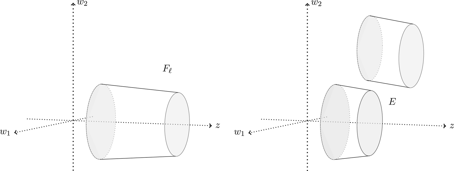
Figure 1. The symmetric set $F_{\ell }$ (left) of an $\ell$
 -distrubuted set $E$
 (right) in case of $n=3$
 . Note that, in general the slices of the set $E$
 do not need to be disks.
This is the $\ell$ -distributed set whose cross sections are $(n-1)$
 -dimensional open balls centred at the $z$
 axis. We notice that the Schwarz symmetric set $F_{\ell }$
 of an $\ell$
 -distributed set $E$
 depends only on the function $\ell$
 , and not on the particular $\ell$
 -distributed set $E$
 under consideration.
Due to Fubini's theorem, Schwarz symmetrization preserves the volume, i.e. if $E$ is $\ell$
 -distributed and $\mathcal {H}^{n} (E) < \infty$
 , it turns out that $\mathcal {H}^{n} (E) =\mathcal {H}^{n}(F_{\ell }).$
 Moreover, the perimeter inequality under Schwarz symmetrization holds, that is

see, for instance, [Reference Brock and Solynin3]. Here, $P(E)$ stands for the perimeter of $E$
 in $\mathbb {R}^{n}$
 (see § 2.4). Additionally, a localized version of (1.5) holds, that is, if $E$
 is a set of finite perimeter, then

for every Borel set $B \subset \mathbb {R}$ , see [Reference Barchiesi, Cagnetti and Fusco2, Theorem 1.1].
The inequality (1.6) is well-known in the literature (see, for instance, [Reference Brock and Solynin3], where this is proved through a careful approximation by polarizations). In [Reference Barchiesi, Cagnetti and Fusco2], one can find an alternative and direct proof, which allowed the authors to give sufficient conditions for rigidity of Steiner's inequality of a general higher codimension $k$ , where $1< k \leq n-1$
 .
.
1.2. Rigidity for perimeter inequality under Schwarz symmetrization
We shall now describe the main objective of the present paper. Given a Lebesgue measurable function $\ell : \mathbb {R} \rightarrow [0,\,\infty )$ , such that $F_{\ell }$
 is a set of finite perimeter and finite volume, we define the class of equality cases of (1.6) as

Due to the invariance of the perimeter under translations along a direction $\tau \in \mathbb {R}^{n-1}$ , as well as the definition of the symmetric set $F_{\ell }$
 , the following inclusion is always true:

where $\triangle$ denotes the symmetric difference of sets. We say that rigidity holds for (1.6) if the opposite inclusion is also satisfied, i.e.

1.3. State of the art
Let us now give an account of the available results in the literature for the rigidity of (1.6). In general, not all equality cases of (1.6) can be written as a translation of the symmetric set $F_{\ell }$ . This can happen, for instance, if the (reduced) boundary $\partial ^{*} F_{\ell }$
 of $F_{\ell }$
 contains flat vertical parts. In such a case, we can find an $\ell$
 -distributed set $E$
 which preserves perimeter under symmetrization, and it is not equivalent to (a translation of) the symmetric set $F_{\ell }$
 ; see Figure 2.


In order to rule out this issue, the authors in [Reference Barchiesi, Cagnetti and Fusco2] localized the problem, by considering an open set $\Omega \subset \mathbb {R}$ , and imposing the following condition:

where $\nu _{w}^{F_{\ell }}(z,\,w)$ denotes the $w$
 -component of the measure-theoretic outer unit normal to the symmetric set $F_{\ell }$
 . It turns out that (1.9) is related to the regularity of the function $\ell$
 . Note that, in general, if $E$
 is a set of finite perimeter in $\mathbb {R}^{n}$
 , then either $F_{\ell }$
 is equivalent to $\mathbb {R}^{n}$
 , or $\ell$
 is a function of Bounded Variation in $\mathbb {R}$
 (see proposition 2.2).
In [Reference Barchiesi, Cagnetti and Fusco2, Proposition 3.5], the authors showed that (1.9) is equivalent to asking that $\ell$ is a Sobolev function in $\Omega$
 , as explained below.
Proposition 1.1 Let $\ell : \mathbb {R}\rightarrow [0,\, \infty )$ be a measurable function, such that $F_{\ell }$
 is a set of finite perimeter and finite volume in $\mathbb {R}^{n}$
 and let $\Omega \subset \mathbb {R}$
 be an open set. Then

if and only if

Even if condition (1.9) (or, equivalently, (1.10)) is satisfied, rigidity can still be violated. In particular, this can happen when the symmetric set $F_{\ell }$ is not connected in a suitable measure-theoretic way, despite the fact that it can be connected from a topological point of view; see Figure 3.


Note that, once condition (1.9) [or, equivalently, (1.10) is imposed, we have that $\ell \in W^{1,1} (\Omega )$ , and since $\Omega$
 is a one-dimensional set, $\ell$
 is absolutely continuous in $\Omega$
 . Therefore the condition imposed in [Reference Barchiesi, Cagnetti and Fusco2] to rule out situations as in Figure 3 can be written as

where $\ell ^{*}$ denotes the Lebesgue representative of $\ell$
 , see [Reference Barchiesi, Cagnetti and Fusco2, condition (1.4)].
It turns out that (1.9) and (1.11) are sufficient for rigidity (see [Reference Barchiesi, Cagnetti and Fusco2, Theorem 1.2]), as explained below.
Theorem 1.2 Let $\ell : \mathbb {R} \rightarrow [0,\, \infty )$ be a measurable function, such that $F_{\ell }$
 is a set of finite perimeter and finite volume. Let $\Omega \subset \mathbb {R}$
 be a connected open set, and suppose that (1.9) and (1.11) are satisfied. If

then $E \cap ( \Omega \times \mathbb {R} )$ is equivalent to (a translation along $\mathbb {R}^{n-1}$
 ) of $F_{\ell } \cap ( \Omega \times \mathbb {R})$
 . Here, $P(E; \Omega \times \mathbb {R})$
 denotes the relative perimeter of $E$
 in $\Omega \times \mathbb {R}$
 .
.
1.4. The main result
Our contribution is to show that conditions (1.9) and (1.11) are also necessary for rigidity. As we have already observed, the proof of the theorem 1.2 requires the localization of the problem in an open and connected set $\Omega \subset \mathbb {R}$ , to impose the condition (1.10). We will show that this can be avoided. We also notice that, if $F_{\ell }$
 is a set of finite perimeter and finite volume, in general, we only have that $\ell \in BV(\mathbb {R})$
 and this means that $\ell$
 may be discontinuous. Therefore, we need to rephrase condition (1.11) in terms of the approximate $\liminf$ $\ell ^{\wedge }$
 of $\ell$
 at every point $z \in \mathbb {R}$
 , see § 2. We are now able to state our main result. Below, $\mathring {J}$
 denotes the interior of $J$
 .
.
Theorem 1.3 Let $\ell : \mathbb {R}\rightarrow [0,\, \infty )$ be a measurable function, such that $F_{\ell }$
 is a set of finite perimeter and finite volume. Then, the following statements are equivalent$:$
(i) (ℛ𝒮) holds true;
(ii) $\{ \ell ^{\wedge } >0\}$
 is a (possibly unbounded) interval $J$ and $\ell \in W^{1,1}(\mathring {J})$.


As we have already pointed out, the proof of the direction $(ii) \Longrightarrow (i)$ of theorem 1.3 relies on the proof of [Reference Barchiesi, Cagnetti and Fusco2, Theorem 1.2]. We will prove that the converse $(i) \Longrightarrow (ii)$
 is also true. We highlight the fact that our approach is not based on a comprehensive use of a general perimeter formula for sets $E \subset \mathbb {R}^{n}$
 satisfying equality in (1.6), as it appears in [Reference Cagnetti, Colombo, De Philippis and Maggi6]. On the contrary, inspired by the techniques developed in [Reference Cagnetti, Perugini and Stöger7], we analyse the properties of the function $\ell$
 and we provide a careful study of the transformations that can be applied on the symmetric set $F_{\ell }$
 , without creating any perimeter contribution.
To this end, the rest of the paper is structured as follows. In § 2, we fix the notation, build the necessary background and we gather some preliminary results that appeared in the literature. In § 3, we show the direction $(i) \Longrightarrow (ii)$ of theorem 1.3, by studying the properties of the distribution function $\ell,$
 and exploiting counterexamples where rigidity is violated.
2. Background and proof of the theorem 1.3 $(ii) \Longrightarrow (i)$

In this section, we will recall the necessary machinery, which will be used throughout the paper. The interested reader could refer to [Reference Ambrosio, Fusco and Pallara1, Reference Barchiesi, Cagnetti and Fusco2, Reference Evans and Gariepy12, Reference Federer13, Reference Maggi17, Reference Simon23].
We fix $n\in \mathbb {N}$ with $n \geq 2$
 . For each $x \in \mathbb {R}^{n}$
 , we write $x=(z,\,w)$
 , with $z \in \mathbb {R}$
 and $w \in \mathbb {R}^{n-1}$
 . The standard Euclidean norm will be denoted by $|\cdot |$
 in $\mathbb {R},\, \ \mathbb {R}^{n-1}$
 or $\mathbb {R}^{n}$
 depending on the context. For $1 \leq m \leq n$
 , we will denote the $m$
 -dimensional Hausdorff measure in $\mathbb {R}^{n}$
 by $\mathcal {H}^{m}.$
 For every radius $\rho >0$
 and $x \in \mathbb {R}^{n}$
 we write $B_{\rho }(x)$
 for the open ball of $\mathbb {R}^{n}$
 with radius $\rho$
 and centred at $x$
 . The volume of the unit ball in $\mathbb {R}^{n}$
 is denoted as $\omega _{n}$
 , i.e., $\omega _{n}:= \mathcal {H}^{n} (B_{1}(0))$
 . Note that throughout the paper, in case of balls in different dimensions, we will denote the corresponding ball in dimension $m$
 with radius $\rho$
 centred at $w \in \mathbb {R}^{m}$
 by writing $B^{m}(w,\,\rho )$
 .
.
Now, for $x \in \mathbb {R}^{n}$ and $\nu \in \partial B_{1}(0)$
 , we set

and

Let $\{E_{j} \} _{j \in \mathbb {N}}$ be a sequence of Lebesgue measurable sets in $\mathbb {R}^{n}$
 with $\mathcal {H}^{n} (E_{j}) < \infty$
 for every $j \in \mathbb {N}$
 , and let $E \subset \mathbb {R}^{n}$
 be a Lebesgue measurable set with $\mathcal {H}^{n} (E) < \infty$
 . We say that $\{ E_{j} \}_{j \in \mathbb {N}}$
 converges to $E$
 as $j \rightarrow \infty$
 and we write

where $\triangle$ stands for the symmetric difference of sets. Additionally, if $E_{1},\, E_{2} \subset \mathbb {R}^{n}$
 are Lebesgue measurable sets, we say that

and

Moreover, the characteristic function of a Lebesgue measurable set $E \subset \mathbb {R}^{n}$ will be denoted by $\chi _{E}$
 .
.
2.1. Density points
Let $E \subset \mathbb {R}^{n}$ be a Lebesgue measurable set and $x \in \mathbb {R}^{n}$
 . We define the lower and upper $n$
 -dimensional densities of $E$
 at $x$
 as
as

respectively. The maps $x \longmapsto \theta _{*} (E,\,x)$ and $x \longmapsto \theta ^{*} (E,\,x)$
 are Borel functions (even in case where $E$
 is Lebesgue non-measurable, see [Reference Simon23, Chapter 1, Remark 3.1]) and they coincide $\mathcal {H}^{n}$
 -a.e. in $\mathbb {R}^{n}$
 . Hence, the $n$
 -dimensional density of $E$
 at $x$
 is defined as the Borel function

For each $s \in [0,\,1],$ we define the set of points of density $s$
 with respect to $E$
 as
as

The essential boundary $\partial ^{e}E$ of $E$
 is defined as the set

2.2. Approximate limits of measurable functions
Let $g: \mathbb {R}^{n} \rightarrow \mathbb {R}$ be a Lebesgue measurable function. We define the approximate upper limit $g^{\vee }(x)$
 and the approximate lower limit $g^{\wedge }(x)$
 of $g$
 at $x \in \mathbb {R}^{n}$
 as
as

and

respectively. We highlight the fact that both $g^{\vee }$ and $g^{\wedge }$
 are Borel functions and they are defined for every $x \in \mathbb {R}^{n}$
 with values in $\mathbb {R} \cup \{ \pm \infty \}.$
 In addition, if $g_{1}: \mathbb {R}^{n} \rightarrow \mathbb {R}$
 and $g_{2}: \mathbb {R}^{n} \rightarrow \mathbb {R}$
 are measurable functions such that $g_{1} = g_{2}$ $\mathcal {H}^{n}$
 -a.e. on $\mathbb {R}^{n}$
 , then it turns out that

The approximate discontinuity set $S_{g}$ of $g$
 is defined as

and satisfies $\mathcal {H}^{n} (S_{g}) =0.$ Moreover, even if $g^{\wedge },\, \ g^{\vee }$
 could take values $\pm \infty$
 on $S_{g}$
 , it turns out that the difference $g^{\vee } - g^{\wedge }$
 is well-defined in $\mathbb {R} \cup \{ \pm \infty \}$
 for every point $x \in S_{g}$
 . In the light of the above considerations, the approximate jump $[\, g \,]$
 of $g$
 is the Borel function $[\, g \,]:\mathbb {R}^{n} \rightarrow [0,\,\infty ]$
 defined as

Let $E\subset \mathbb {R}^{n}$ be a Lebesgue measurable set. We will say that $s \in \mathbb {R} \cup \{ \pm \infty \}$
 is the approximate limit of $g$
 at $x$
 with respect to $E$
 , denoted by $s = \text {aplim} (g ,\, E,\, x)$
 , if
, if


and

We will say that $x \in S_{g}$ is a jump point of $g$
 if there exist $\nu \in \partial B_{1}(0)$
 such that

In this spirit, we define the approximate jump direction $\nu _{g}(x)$ of $g$
 at $x$
 as $\nu _{g}(x):=\nu$
 . The set of approximate jump points of $g$
 is denoted by $J_{g}$
 . Note that $J_{g} \subset S_{g}$
 and $\nu _{g} : J_{g} \rightarrow \partial B_{1}(0)$
 is a Borel function.
2.3. Functions of bounded variation
Let $\Omega \subset \mathbb {R}^{n}$ be an open set. We denote by $C_{c}^{1}( \Omega ; \mathbb {R}^{n})$
 and by $C_{c}( \Omega ; \mathbb {R}^{n})$
 the class of $C^{1}$
 functions with compact support and the class of all continuous functions with compact support from $\Omega$
 to $\mathbb {R}^{n}$
 , respectively. We also recall the Sobolev space $W^{1,1} (\Omega )$
 , that is, the space of all functions $g \in L^{1} (\Omega )$
 , whose distributional derivative $Dg$
 belongs to $L^{1} (\Omega )$
 .
.
Given $g \in L^{1} (\Omega )$ , the total variation of $g$
 in $\Omega$
 is defined as

We then define the space of functions of bounded variation in $\Omega$ , denoted by $BV(\Omega )$
 , as the set of functions $g \in L^{1} (\Omega )$
 such that $|Dg|(\Omega ) <\infty$
 . In addition, we will say that $g \in BV_{loc} (\Omega )$
 , if $g \in BV(\Omega ')$
 for every $\Omega ' \subset \subset \Omega$
 . If $g \in BV(\Omega )$
 , due to Radon-Nikodym decomposition of $D g$
 with respect to $\mathcal {H}^{n}$
 , we have

where $D^{a}g$ and $D^{s}g$
 are mutually singular measures and $D^{a}g \ll \mathcal {H}^{n}$
 . The density of $D^{a}g$
 with respect to $\mathcal {H}^{n}$
 will be denoted as $\nabla g$
 , and we have that $\nabla g \in L^{1} (\Omega,\, \mathbb {R}^{n})$
 with $D^{a}g = \nabla g \ d \mathcal {H}^{n}$
 . Additionally, it turns out that $\mathcal {H}^{n-1} ( S_{g} \backslash J_{g} ) = 0$
 and $[\, g\, ] \in L^{1}_{loc} ( \mathcal {H}^{n-1} \llcorner J_{g})$
 , see [Reference Ambrosio, Fusco and Pallara1, Theorem 3.78]. The jump part of $g$
 is the $\mathbb {R}^{n}$
 -valued Radon measure given by

Finally, the Cantorian part $D^{c}g$ of $Dg$
 is defined as the $\mathbb {R}^{n}$
 -valued Radon measure

and is such that $|D^{c}g | (N)=0$ for every set $N \subset \mathbb {R}^{n}$
 , which is $\sigma$
 -finite with respect to $\mathcal {H}^{n-1}$
 , see [Reference Ambrosio, Fusco and Pallara1, Proposition 3.92].
Note, that in the special case $n=1$ , if $(a,\,b) \subset \mathbb {R}$
 is an open interval, every $g \in BV(a,\,b)$
 can be decomposed as the sum

where $g^{a} \in W^{1,1} (a,\,b)$ , $g^{j}$
 is a purely jump function (that is, $D g^{j} = D^{j}g^{j})$
 and $g^{c}$
 is a purely Cantorian function (that is, $Dg^{c} = D^{c}g^{c}$
 ), see [Reference Ambrosio, Fusco and Pallara1, Corollary 3.33]. Moreover, if $g$
 is a good representative (see [Reference Ambrosio, Fusco and Pallara1, Theorems 3.27, 3.28]), then the total variation $|Dg|$
 of $Dg$
 can be written as

where the supremum is taken over all $M \in \mathbb {N}$ and over all possible partitions of the interval $(a,\,b)$
 with $a< x_{1} < x_{2} < \cdots < x_{M} < b$
 .
.
2.4. Sets of locally finite perimeter in the Euclidean space
Let $n,\,m \in \mathbb {N}$ with $1\leq m \leq n$
 . Let also $E \subset \mathbb {R}^{n}$
 be an $\mathcal {H}^{m}$
 -measurable set. We say that $E$
 is a countably $\mathcal {H}^{m}$
 -rectifiable set if there exists a countable family of Lipschitz functions $(g_{j})_{j \in \mathbb {N}}$
 , where $g_{j}: \mathbb {R}^{m} \rightarrow \mathbb {R}^{n}$
 , such that $E \subset _{\mathcal {H}^{m}} \bigcup _{j \in \mathbb {N}} g_{j} (\mathbb {R}^{m})$
 . In addition, if $\mathcal {H}^{m} ( E \cap K) < \infty$
 for every compact set $K \subset \mathbb {R}^{n}$
 , we say that $E$
 is a locally $\mathcal {H}^{m}$
 -rectifiable set.
Let $E \subset \mathbb {R}^{n}$ be a Lebesgue measurable set. We say that $E$
 is a set of locally finite perimeter in $\mathbb {R}^{n}$
 if there exists an $\mathbb {R}^{n}$
 -valued Radon measure $\mu _{E}$
 , such that

Note that, $E$ is a set of locally finite perimeter if and only if $\chi _{E} \in BV_{loc} (\mathbb {R}^{n})$
 . If $G \subset \mathbb {R}^{n}$
 is a Borel set, then the relative perimeter of $E$
 in $G$
 is defined as

When $G=\mathbb {R}^{n}$ , we ease the notation to $P(E):=P(E; \mathbb {R}^{n})$
 .
.
The reduced boundary $\partial ^{*}E$ of $E$
 is the set of all $x\in \mathbb {R}^{n}$
 such that

The Borel function $\nu _{E}: \partial ^{*} E \rightarrow \partial B_{1}(0)$ is usually referred to as the measure-theoretic outer normal to $E$
 . Due to Lebesgue-Besicovitch derivation theorem and [Reference Ambrosio, Fusco and Pallara1, Theorem 3.59], it holds that the reduced boundary $\partial ^{*}E$
 of $E$
 is a locally $(n-1)$
 -rectifiable set in $\mathbb {R}^{n}$
 and
and

so that

Thus, for every Borel set $G \subset \mathbb {R}^{n}$ we have that

Finally, if $E$ is a set of locally finite perimeter, it holds

and additionally, thanks to Federer's theorem (see e.g., [Reference Ambrosio, Fusco and Pallara1, Theorem 3.61] or [Reference Maggi17, Theorem 16.2]), we have that

which implies that the essential boundary $\partial ^{e}E$ of $E$
 is locally $\mathcal {H}^{n-1}$
 -rectifiable in $\mathbb {R}^{n}$
 .
.
2.5. Preliminary results
In this final subsection, we state some results which will be useful in the following.
The first significant result relates to the set $E_{z}$ defined in (1.1). Namely, as it turns out, for $\mathcal {H}^{1}$
 -a.e $z \in \mathbb {R}$
 , $E_{z}$
 is a set of finite perimeter and its reduced boundary $\partial ^{*} (E_{z})$
 enjoys an advantageous property. These facts follow due to a variant of a result by Vol'pert [Reference Vol'pert26], which is provided in [Reference Barchiesi, Cagnetti and Fusco2, Theorem 2.4].
Proposition 2.1 Vol'pert
Let $E$ be a set of finite perimeter in $\mathbb {R}^{n}$
 . Then for $\mathcal {H}^{1}$
 -a.e. $z \in \mathbb {R}$
 the following hold true$:$
(i) $E_{z}$
is a set of finite perimeter in $\mathbb {R}^{n-1}$;(ii) $\mathcal {H}^{n-2}((\partial ^{*} E)_{z} \triangle \partial ^{*} (E_{z}))=0$
.


Thanks to $(ii)$ above, we will often write $\partial ^{*} E_{z}$
 instead of $(\partial ^{*} E)_{z}$
 or $\partial ^{*} (E_{z})$
 . The next result presents a crucial regularity property of the function $\ell$
 , and it can be found in [Reference Barchiesi, Cagnetti and Fusco2, Lemma 3.1].
Proposition 2.2 Let $E$ be a set of finite perimeter in $\mathbb {R}^{n}$
 . Then either $\ell (z) =\infty$
 for $\mathcal {H}^{1}$
 -a.e. $z \in \mathbb {R}$
 , or $\ell (z) < \infty$
 for $\mathcal {H}^{1}$
 -a.e. $z \in \mathbb {R}$
 and $\mathcal {H}^{n} (E) < \infty$
 . In the latter case, we have $\ell \in BV(\mathbb {R} )$
 .
.
We present the following auxiliary inequality, which is a special case of [Reference Barchiesi, Cagnetti and Fusco2, Proposition 3.4].
Proposition 2.3 Let $\ell :\mathbb {R} \rightarrow [0,\, \infty )$ be a measurable function, such that $F_{\ell }$
 is a set of finite perimeter and finite volume. Let $E \subset \mathbb {R}^{n}$
 be an $\ell$
 -distributed set and let $f: \mathbb {R} \rightarrow [0,\,\infty ]$
 be a Borel measurable function. Then

Moreover, if $E = F_{\ell },$ the equality holds in (2.9).
A straightforward consequence of the above result is the following.
Corollary 2.4 Let $\ell : \mathbb {R}\rightarrow [0,\, \infty )$ be a measurable function, such that $F_{\ell }$
 is a set of finite perimeter and finite volume. Then

for every Borel set $B \subset \mathbb {R}$ .
.
For sake of completeness, we close this preliminary section by presenting the proof of theorem 1.3 $(ii) \Longrightarrow (i)$ .
.
Proof Proof of theorem 1.3 $(ii) \Longrightarrow (i)$
Suppose that $(ii)$ holds. Since $\ell \in W^{1,1}(\mathring {J})$
 , by proposition 1.1, the condition (ℛ𝒮) is satisfied with $\Omega = \mathring {J}$
 . In addition, since $J$
 is one-dimensional, $\ell$
 is absolutely continuous in $\mathring {J}$
 and therefore,

where $\ell ^{*}$ stands for the Lebesgue representative of $\ell$
 . Thus, it turns out that (1.11) is true. Therefore, due to theorem 1.2, $(i)$
 follows.
3. Proof of the theorem 1.3 $(i) \Longrightarrow (ii)$

We start our analysis with the following lemma, which will be extensively used in the sequel.
Lemma 3.1 Let $\ell : \mathbb {R}\rightarrow [0,\, \infty )$ be a measurable function, such that $F_{\ell }$
 is a set of finite perimeter and finite volume. Let also $r_{\ell }$
 be defined as in (1.3) and consider $\bar {z} \in \mathbb {R}.$
 Then
Then

Proof. The proof is divided into two steps.
Step 1: We prove
(3.2)\begin{equation} ( \partial^{*} F_{\ell})_{\bar{z}} \subset \overline{B^{n-1} ( 0 , r_{\ell}^{{\vee}}(\bar{z}))} \backslash B^{n-1} ( 0 , r_{\ell}^{{\wedge}}(\bar{z})). \end{equation}To this end, it is enough to prove that
(3.3a)\begin{equation} r_{\ell}^{{\wedge}}(\bar{z}) \leq |w| \quad \text{for every } w \in (\partial^{*} F_{\ell})_{\bar{z}} \end{equation}and
(3.3b)\begin{equation} r_{\ell}^{{\vee}}(\bar{z}) \geq |w| \quad \text{for every } w \in (\partial^{*} F_{\ell})_{\bar{z}}. \end{equation}
First, we prove (3.3a). To achieve that, we observe that (3.3a) will follow by proving the implication:
\[ r_{\ell}^{{\wedge}}(\bar{z}) > |w| \Longrightarrow (\bar{z},w) \in F_{\ell}^{(1)}, \]or equivalently,
\[ r_{\ell}^{{\wedge}}(\bar{z}) > |w| \Longrightarrow (\bar{z},w) \in (\mathbb{R}^{n} \backslash F_{\ell})^{(0)}. \]
To this aim, let $w \in \mathbb {R}^{n-1}$
be such that $r_{\ell }^{\wedge } (\bar {z}) > |w|$, and let $\delta >0$ be such that
\[ r_{\ell}^{{\wedge}}(\bar{z}) = |w| + \delta. \]Let now $\bar {\rho } \in (0,\, {\delta }/{2}]$
. Then,
\[ |w-w'| < \bar{\rho} \leq \frac{\delta}{2} \quad \text{for every } (z',w') \in B_{\bar{\rho}} ( (\bar{z},w)). \]By virtue of the triangle inequality, we have
\[ r_{\ell}^{{\wedge}}(\bar{z}) = |w| + \delta \geq |w'| -|w-w'| + \delta > |w'| + \frac{ \delta}{2}, \]so that
(3.4)\begin{equation} r_{\ell}^{{\wedge}}(\bar{z}) - \frac{\delta}{2} > |w'| \quad \text{for every } (z',w') \in B_{\bar{\rho}} ( (\bar{z},w)) . \end{equation}
Now, thanks to (3.4) and the definition of $F_\ell$
, we have
\begin{align*} & (\mathbb{R}^{n} \backslash F_\ell ) \cap B_{\bar{\rho}} ( (\bar{z},w) )\\ & \quad \subset \left\{ (z',w') \in \mathbb{R} \times \mathbb{R}^{n-1}: r_{\ell}^{{\wedge}}(\bar{z}) - \frac{\delta}{2} > |w'| \geq r_{\ell}(z') \right\} \cap B_{\bar{\rho}} ( (\bar{z},w) ). \end{align*}Hence, for every $\rho \in (0,\, \bar {\rho })$
, we have
\begin{align*} & \mathcal{H}^{n} ( (\mathbb{R}^{n} \backslash F_\ell) \cap B_{\rho} ( (\bar{z},w) ) )\\ & \quad = \int_{\bar{z} - \rho}^{\bar{z} + \rho} \mathcal{H}^{n-1} ( (\mathbb{R}^{n} \backslash F_\ell ) \cap B_{\rho} ( (\bar{z},w)) \cap \{ z = \zeta\} )\,{\rm d} \zeta \\ & \quad \leq \int_{\bar{z} - \rho}^{\bar{z} + \rho} \chi_{ \left\{ r_{\ell} < r_{\ell}^{{\wedge}}(\bar{z}) - \frac{\delta}{2} \right\}} (\zeta) \mathcal{H}^{n-1} ( (\mathbb{R}^{n} \backslash F_\ell ) \cap B_{\rho}((\bar{z},w)) \cap \{z = \zeta\})\,{\rm d}\zeta \\ & \quad = \int_{ ( \bar{z} - \rho, \bar{z} + \rho) \cap \left\{ r_{\ell} < r_{\ell}^{{\wedge}}(\bar{z}) - \frac{\delta}{2} \right\}} \mathcal{H}^{n-1} ( (\mathbb{R}^{n} \backslash F_\ell )\cap B_{\rho}(( \bar{z},w)) \cap \{z = \zeta\})\,{\rm d} \zeta. \end{align*}Now, for $\rho \in (0,\, \bar {\rho })$
and for every $\zeta \in ( \bar {z} - \rho,\, \bar {z} + \rho )$, we observe that,
\[ B_{\rho} ( (\bar{z},w)) \cap \{ z = \zeta\} \subset \left\{ (z,w_{0}) \in \mathbb{R} \times \mathbb{R}^{n-1} : z= \bar{z} \text{ and } w_{0} \in B^{n-1} (w,\rho)\right\}. \]Therefore, for $\rho \in (0,\, \bar {\rho })$
we obtain
\begin{align*} & \mathcal{H}^{n} ( (\mathbb{R}^{n} \backslash F_\ell ) \cap B_{\rho} ( (\bar{z},w))) \\ & \leq \int_{ ( \bar{z} - \rho, \bar{z} + \rho) \cap \left\{ r_{\ell} < r_{\ell}^{{\wedge}}(\bar{z}) - \frac{\delta}{2} \right\}} \mathcal{H}^{n-1} (B^{n-1} ( w, \rho ) )\,{\rm d} \zeta\\ & = \omega_{n-1} \rho^{n-1} \int_{ ( \bar{z} - \rho, \bar{z} + \rho) \cap \left\{ r_{\ell} < r_{\ell}^{{\wedge}}(\bar{z}) - \frac{\delta}{2} \right\}} 1\,{\rm d} \zeta \\ & = \omega_{n-1} \rho^{n-1} \ \mathcal{H}^{1} (( \bar{z} - \rho, \bar{z} + \rho) \cap \left\{ r_{\ell} < r_{\ell}^{{\wedge}}(\bar{z}) - \frac{\delta}{2} \right\} ). \end{align*}
Finally, we have
\begin{align*} & \lim_{ \rho \rightarrow 0^+} \frac{ \mathcal{H}^{n} ( (\mathbb{R}^{n} \backslash F_\ell) \cap B_{\rho}( (\bar{z},w)))}{\omega_{n} \rho^{n} } \\ & \leq \frac{ \omega_{n-1}}{\omega_{n}} \lim_{ \rho \rightarrow 0^+} \frac{ \mathcal{H}^{1} (( \bar{z} - \rho, \bar{z} + \rho) \cap \left\{ r_{\ell} < r_{\ell}^{{\wedge}}(\bar{z}) - \frac{\delta}{2} \right\} )}{ \rho} \\ & =0, \end{align*}where in the last equality we make use of the definition of $r_{\ell }^{\wedge }(\bar {z})$
, see (2.2). This shows (3.3a). Employing an analogous argument, it can be shown that
\[ r_{\ell}^{{\vee}}(\bar{z}) < |w| \Longrightarrow (\bar{z},w) \in F_{\ell}^{(0)}. \]This implies (3.3b), and finally proves (3.2). For a graphical illustration of Step 1, see Figure 4.
Step 2: We conclude the proof. We first observe that by corollary 2.4 with $B=\{\bar {z}\}$
, we obtain
\begin{align*} \mathcal{H}^{n-1} ( ( \partial^{*} F_{\ell})_{\bar{z}} ) & = \mathcal{H}^{n-1} ( \partial^{*} F_{\ell} \cap \{ z= \bar{z} \} ) \\ & = \mathcal{H}^{n-1} ( \partial^{*} F_{\ell} \cap ( \{ \bar{z} \} \times \mathbb{R}^{n-1})) \\ & = P (F_{\ell}; \{ \bar{z} \} \times \mathbb{R}^{n-1})\\ & = \ell^{{\vee}}(\bar{z}) - \ell^{{\wedge}}(\bar{z}) \\ & = \mathcal{H}^{n-1} (\overline{ B^{n-1} (0, r_{\ell}^{{\vee}}(\bar{z}))} )- \mathcal{H}^{n-1} ( B^{n-1} ( 0, r_{\ell}^{{\wedge}}(\bar{z}))) \\ & = \mathcal{H}^{n-1} (\overline{ B^{n-1} ( 0, r_{\ell}^{{\vee}}(\bar{z}))} \big\backslash ( B^{n-1} ( ( 0, r_{\ell}^{{\wedge}}(\bar{z}))) ). \end{align*}
Figure 4. A graphical illustration of Step 1 for $n=3$
.Finally, recalling that, by Step 1
\[ ( \partial^{*} F_{\ell})_{\bar{z}} \subset \overline{B^{n-1} ( 0 , r_{\ell}^{{\vee}}(\bar{z}))} \backslash B^{n-1} ( 0 , r_{\ell}^{{\wedge}}(\bar{z})), \]we obtain
\begin{align*} (\partial^{*} F_{\ell} )_{\bar{z}}& =_{\mathcal{H}^{n-1}} \overline{B^{n-1} ( 0 , r_{\ell}^{{\vee}}(\bar{z}))} \backslash B^{n-1} ( 0 , r_{\ell}^{{\wedge}}(\bar{z})) \\ & =_{\mathcal{H}^{n-1}} B^{n-1} ( 0, r_{\ell}^{{\vee}}(\bar{z})) \backslash B^{n-1} ( 0 , r_{\ell}^{{\wedge}}(\bar{z})), \end{align*}which concludes the proof.


Now, we can show that if the set $\{\ell ^{\wedge } >0 \}$ fails to be a (possibly unbounded) interval, then rigidity is violated.
Proposition 3.2 Let $\ell : \mathbb {R}\rightarrow [0,\, \infty )$ be a measurable function, such that $F_{\ell }$
 is a set of finite perimeter and finite volume, and let $r_{\ell }$
 be defined as in (1.3). Suppose that the set $\{ \ell ^{\wedge } >0 \}$
 is not an interval. That is, suppose that there exists $\bar {z} \in \{ \ell ^{\wedge }=0\}$
 such that

Then, rigidity is violated. More precisely, setting $E_{1}:= F_{\ell } \cap \{ z < \bar {z} \}$ and $E_{2} = F_{\ell } \backslash E_{1},$
 then
then

Proof. Let $E_{1},\, \ E_{2}$ and $E$
 be as in the statement. Let also $\tau \in \mathbb {R}^{n-1}$
 . First of all, note that, since $\{z < \bar {z}\}$
 is open and $E \cap \{z < \bar {z}\}= F_{\ell } \cap \{z < \bar {z}\}$
 , we have

for every $s \in [0,\,1].$ In accordance of that, we infer

In the same fashion, for every $\tau \in \mathbb {R}^{n-1}$ , we obtain

Hence, due to (3.5) and (3.6), we have

As a consequence, in order to complete the proof, we need to show that

In what will follow, without loss of generality we assume that

We divide the proof of (3.7) in several steps.
Step 1: We show that
(3.9)\begin{equation} ( \partial^{*} E)_{\bar{z} } \subset \overline{B^{n-1} ( 0 , r_{\ell}^{{\vee}} (\bar{z}))} \cup \{ \tau \}. \end{equation}
To this end, it suffices to prove that
(3.10)\begin{equation} |w| \leq r_{\ell}^{{\vee}}( \bar{z} ) \quad \text{ for every } w \in (\partial^{*} E )_{\bar{z}} \backslash \{ \tau \} . \end{equation}
Step 1a: We show that
\[ |w| > r_{\ell}^{{\vee}} (\bar{z}) \Longrightarrow (\bar{z},w) \ \in E_{1}^{(0)}. \]To this aim, suppose that there exists $\delta >0$
such that
\[ |w| = r_{\ell}^{{\vee}} ( \bar{z}) + \delta. \]Then, by arguing as in Step 1 of lemma 3.1, for every $\bar {\rho } \in (0,\, {\delta }/{2})$
we obtain
\[ |w'| > r_{\ell}^{{\vee}} ( \bar{z}) + \frac{\delta}{2} \quad \text{ for every } (z',w') \in B_{\bar{\rho}}((\bar{z},w)). \]So, by the definition of $E_{1},$
we have
\begin{align*} & E_{1} \cap B_{\bar{\rho}}((\bar{z},w)) = F_{\ell} \cap \{ z< \bar{z} \} \cap B_{\bar{\rho}}((\bar{z},w)) \\ & \subset \left\{ (z',w') \in \mathbb{R}\times \mathbb{R}^{n-1} : z' < \bar{z} \ \text{and} \ r_{\ell}^{{\vee}} (\bar{z}) + \frac{\delta}{2} < |w'| < r_{\ell} (z') \right\} \cap B_{\bar{\rho}}((\bar{z},w)). \end{align*}
Thus, for every $\rho \in ( 0 ,\, \bar {\rho })$
, by similar calculations as in Step 1 of lemma 3.1, we obtain
\begin{align*} & \lim_{ \rho \rightarrow 0^+} \frac{\mathcal{H}^{n}(E_{1} \cap B_{\rho} ((\bar{z},w)) )}{\omega_{n} \rho^{n}} \\ & \leq \frac{1}{ \omega_{n}} \lim_{ \rho \rightarrow 0^+} \int_{(\bar{z} -\rho, \bar{z}) \cap \{ r_{\ell} > r_{\ell}^{{\vee}} (\bar{z}) +\frac{\delta}{2}\}} \mathcal{H}^{n-1} ( F_{\ell} \cap B_{\rho}((\bar{z},w)) \cap \{ z = \zeta \} )\,{\rm d} \zeta \\ & \leq \frac{ \omega_{n-1}}{\omega_{n}} \lim_{ \rho \rightarrow 0^+} \frac{ \mathcal{H}^{1} ( ( \bar{z} - \rho, \bar{z} ) \cap \left\{ r_{\ell} > r_{\ell}^{{\vee}} (\bar{z}) + \frac{\delta}{2} \right\} )}{\rho} \\ & =0, \end{align*}where in the latter inequality (3.8) has been used.
Step 1b: We show that
(3.11)\begin{equation} \{ z= \bar{z} \} \backslash\{(\bar{z},\tau )\} \subset ( (0, \tau ) + E_{2})^{(0)}. \end{equation}
To this aim, suppose that $\epsilon := | w - \tau | >0.$
We will prove that $(\bar {z},\,w) \in ( (0,\,\tau ) + E_2)^{(0)}.$ Recalling the argument which was used in the proof of (3.4), we choose $\bar {\rho }\in (0,\, {\epsilon }/{2})$ such that
\[ |w' - \tau | > \frac{\epsilon}{2} \quad \text{ for every}\ (z',w') \in B_{\bar{\rho}} ((\bar{z},w)). \]Then, we have
\begin{align*} & ( (0, \tau) + E_{2} ) \cap B_{\bar{\rho}} ((\bar{z},w)) \\ & = ( (0,\tau) + ( F_{\ell} \cap \{ z \geq \bar{z} \}) ) \cap B_{\bar{\rho}} ((\bar{z},w))\\ & \subset \left\{ (z',w') \in \mathbb{R} \times \mathbb{R}^{n-1} : z' \geq \bar{z}, \ \ \frac{\epsilon}{2} < |w' - \tau | < r_{\ell} (z')\right\} \cap B_{\bar{\rho}} ((\bar{z},w)). \end{align*}
Now, for $\rho \in (0,\, \bar {\rho })$
and for every $\zeta \in ( \bar {z} - \rho,\, \bar {z} + \rho )$, we note that,
\[ B_{\rho} ( (\bar{z},w)) \cap \{ z = \zeta\} \subset \left\{ (z,w_{0}) \in \mathbb{R} \times \mathbb{R}^{n-1} : z= \bar{z} \text{ and } w_{0} \in B^{n-1} (w,\rho)\right\}. \]Thus, for every $\rho \in (0 ,\, \bar {\rho })$
,
\begin{align*} \mathcal{H}^{n} ((0, \tau ) + E_{2} ) \cap B_{\rho} ( ( \bar{z} ,w))) & \leq \int_{ ( \bar{z} , \bar{z} + \rho) \cap \{ r_{\ell} > \frac{\epsilon}{2} \}} \mathcal{H}^{n-1} (B^{n-1} ( w, \rho ) )\,{\rm d} \zeta \\ & = \omega_{n-1} \rho^{n-1} \int_{ ( \bar{z}, \bar{z} + \rho) \cap \{ r_{\ell} > \frac{\epsilon}{2} \} } 1\,{\rm d} \zeta \\ & = \omega_{n-1} \rho^{n-1} \ \mathcal{H}^{1} (( \bar{z}, \bar{z} + \rho) \cap \left\{ r_{\ell} > \frac{\epsilon}{2} \right\} ). \end{align*}
Based on this, by (3.8) we infer that
\begin{align*} \lim_{ \rho \rightarrow 0^+} \frac{ \mathcal{H}^{n} ((0, \tau) ) + E_{2} ) \cap B_{\rho} ( ( \bar{z} ,w))) }{ \omega_{n} \rho^{n}} & \leq \frac{ \omega_{n-1}}{\omega_{n}} \lim_{ \rho \rightarrow 0^+} \frac{ \mathcal{H}^{1} (( \bar{z}, \bar{z} + \rho) \cap \left\{ r_{\ell} > \frac{\epsilon}{2} \right\} )}{\rho} \\ & =0, \end{align*}which proves (3.11).
Step 1c: To conclude the proof of Step 1, we observe that, by Step 1a and 1b, as well as by the definition of $E,$
it follows that
\[ \left\{ (\bar{z},w) \in \mathbb{R} \times \mathbb{R}^{n-1} : |w| > r_{\ell}^{{\vee}} (\bar{z}) \right\} \bigg\backslash \{ ( \bar{z},\tau ) \} \subset E_{1}^{(0)} \cap ( (0,\tau) +E_{2} )^{(0)} = E^{(0)}. \]
Therefore,
\begin{align*} (\partial^{*}E)_{ \bar{z}} & \subset \mathbb{R}^{n-1} \bigg\backslash ( \left\{ w \in \mathbb{R}^{n-1} : |w| > r_{\ell}^{{\vee}} (\bar{z}) \right\} \bigg\backslash\{ \tau\} ) \\ & = \overline{ B^{n-1} ( 0, r_{\ell}^{{\vee}} (\bar{z}) )}\cup \{ \tau\}, \end{align*}which shows (3.9).
Step 2: Finally, we show (3.7). Note that, thanks to Step 1, lemma 3.1 and perimeter inequality (1.6), we have
\begin{align*} P(E ; \{ z= \bar{z} \} )& = \mathcal{H}^{n-1} ( \partial^{*} E \cap \{z = \bar{z}\}) = \mathcal{H}^{n-1} (( \partial^{*} E )_{\bar{z}}) \\ & \leq \mathcal{H}^{n-1} ( B^{n-1} ( (0, r_{\ell}^{{\vee}} (\bar{z}) ) ) \\ & = \mathcal{H}^{n-1} ( \partial^{*} F_{\ell} \cap \{z = \bar{z} \})\\ & = P (F_{\ell}; \{z=\bar{z} \}) \leq P(E ; \{z= \bar{z} \}), \end{align*}which makes our proof complete.


We will now show that, if the jump part $D^{j} \ell$ of $D \ell$
 is non-zero, then rigidity is violated.
Proposition 3.3 Let $\ell : \mathbb {R}\rightarrow [0,\, \infty )$ be a measurable function, such that $F_{\ell }$
 is a set of finite perimeter and finite volume, and let $r_{\ell }$
 be defined as in (1.3). Suppose that $\ell$
 has a jump at some point $\bar {z} \in \mathbb {R}$
 . Then rigidity is violated. More precisely, setting $E_{1}:= F_{\ell } \cap \{ z < \bar {z} \}$
 and $E_{2} := F_{\ell } \backslash E_{1},$
 then
then

for every $\tau \in \mathbb {R}^{n-1}$ such that

Proof. Let $E_{1},\, \ E_{2}$ and $E$
 be as in the statement. Let also $\tau \in \mathbb {R}^{n-1}$
 be such that (3.12) is satisfied. It is not restrictive to assume that

By an analogous argument as in the beginning of the proof of proposition 3.2, we obtain

Hence, in order to complete the proof, we finally need to show that

We divide the proof of (3.14) into further steps.
Step 1: We prove that
(3.15)\begin{equation} (\partial^{*} E)_{\bar{z}} \subset \overline{B^{n-1} (0, r_{\ell}^{{\vee}}( \bar{z} ))} \backslash B^{n-1} ( \tau , r_{\ell}^{{\wedge}}(\bar{z})). \end{equation}
In order to show (3.15), it suffices to prove that
(3.16a)\begin{equation} r_{\ell}^{{\wedge}} (\bar{z}) \leq |w-\tau| \quad \text{ for every } w \in (\partial^{*} E)_{\bar{z}} \end{equation}and
(3.16b)\begin{equation} r_{\ell}^{{\vee}} (\bar{z}) \geq |w| \quad \text{ for every } w \in (\partial^{*} E)_{\bar{z}}. \end{equation}
First, let us prove (3.16a). To achieve that, we observe, due to (2.7), our claim will follow if we prove that
(3.17)\begin{equation} |w -\tau| < r_{\ell}^{{\wedge}} (\bar{z}) \Longrightarrow (\bar{z},w) \in (\mathbb{R}^{n} \backslash E)^{(0)}. \end{equation}
To this end, suppose that $w \in \mathbb {R}^{n-1}$
is such that $|w -\tau | < r_{\ell }^{\wedge } (\bar {z})$. Then, we observe that
\[ \mathbb{R}^{n} \backslash E = (( \mathbb{R}^{n} \backslash E) \cap \{ z < \bar{z} \}) \cup ( ( \mathbb{R}^{n} \backslash E) \cap \{ z \geq \bar{z}\} ). \]
Now, arguing as in Step 1 of proposition 3.2, we infer that
(3.18)\begin{equation} \lim_{\rho \rightarrow 0^+} \frac{\mathcal{H}^{n} ( (\mathbb{R}^{n} \backslash E)\cap B_{\rho} (( \bar{z},w) \cap \{z < \bar{z} \})} {\omega_{n} \rho^{n}} =0. \end{equation}
Hence, to complete the proof of the claim, it remains to show that
(3.19)\begin{equation} \lim_{\rho \rightarrow 0^+} \frac{\mathcal{H}^{n} ( (\mathbb{R}^{n} \backslash E)\cap B_{\rho} (( \bar{z},w) \cap \{z \geq \bar{z})\}} {\omega_{n} \rho^{n}} =0. \end{equation}Then there exists $\delta >0$
such that
\[ |w-\tau| + \delta = r_{\ell}^{{\wedge}}(\bar{z}). \]Let now $\bar {\rho } \in (0,\, {\delta }/{2}]$
. Then, for each $(z',\,w') \in B_{\bar {\rho }}((\bar {z},\,w))$
\[ r_{\ell}^{{\wedge}} (\bar{z}) \geq |w'-\tau| -|w-w'| + \delta > |w'-\tau| - \frac{\delta}{2} +\delta = |w'-\tau| + \frac{\delta}{2}, \]so that
(3.20)\begin{equation} r_{\ell}^{{\wedge}} (\bar{z}) - \frac{\delta}{2} > |w' - \tau| \quad \text{ for every } (z',w') \in B_{\bar{\rho}}((\bar{z},w)). \end{equation}Then, employing (3.20) and the definition of the set $E$
, we infer
\begin{align*} & (\mathbb{R}^{n} \backslash E)\cap B_{\bar{\rho}}((\bar{z},w)) \cap \{ z \geq \bar{z}\} \\ & \subset \left\{ (z',w') \in \mathbb{R} \times \mathbb{R}^{n-1}: z \geq \bar{z}, \ r_{\ell}^{{\wedge}}(\bar{z}) - \frac{\delta}{2}>|w'-\tau|\geq r_{\ell} (z') \right\} \cap B_{\bar{\rho}}((\bar{z},w)). \end{align*}Moreover, we note that for $\rho \in (0,\, \bar {\rho })$
and for every $\zeta \in ( \bar {z} - \rho,\, \bar {z} + \rho )$, we have
\[ B_{\rho} ( (\bar{z},w)) \cap \{ z = \zeta\} \subset \left\{ (z,w_{0}) \in \mathbb{R} \times \mathbb{R}^{n-1} : z= \bar{z} \text{ and } w_{0} \in B^{n-1} (w,\rho)\right\}. \]As a consequence, for $\rho \in (0,\, \bar {\rho })$
we obtain
\begin{align*} & \mathcal{H}^{n} ((\mathbb{R}^{n} \backslash E)\cap B_{\rho}((\bar{z},w)) \cap \{ z \geq \bar{z}\} ) \\ & \leq \int_{ ( \bar{z} , \bar{z} + \rho) \cap \left\{ r_{\ell}< r_{\ell}^{{\wedge}}(\bar{z}) - \frac{\delta}{2} \right\}} \mathcal{H}^{n-1} (B^{n-1} ( w, \rho ) )\,{\rm d} \zeta\\ & = \omega_{n-1} \rho^{n-1} \int_{ ( \bar{z}, \bar{z} + \rho) \cap \left\{ r_{\ell} < r_{\ell}^{{\wedge}}(\bar{z}) - \frac{\delta}{2} \right\}} 1\,{\rm d} \zeta \\ & = \omega_{n-1} \rho^{n-1} \mathcal{H}^{1} (( \bar{z}, \bar{z} + \rho) \cap \left\{ r_{\ell} < r_{\ell}^{{\wedge}}(\bar{z}) - \frac{\delta}{2} \right\} ). \end{align*}Then, thanks to (3.13), we infer
\begin{align*} & \lim_{\rho \rightarrow 0^+} \frac{\mathcal{H}^{n} ( (\mathbb{R}^{n} \backslash E) \cap B_{\rho} ( (\bar{z},w))\cap \{ z \geq \bar{z}\})}{\omega_{n} \rho^{n}} \\ & \leq \frac{\omega_{n-1}}{\omega_{n}} \lim_{\rho \rightarrow 0^+} \frac{ \mathcal{H}^{1} (( \bar{z}, \bar{z} + \rho) \cap \left\{ r_{\ell} < r_{\ell}^{{\wedge}}(\bar{z}) - \frac{\delta}{2} \right\} )} {\rho} =0, \end{align*}where (2.3b) has been employed. This proves (3.19). Then, combining (3.18) and (3.19), (3.17) follows, and thus the proof of (3.16a) is complete.
Now, for (3.16b), arguing again as in Step 1 of proposition 3.2, we have
(3.21)\begin{equation} |w|> r_{\ell}^{{\vee}} (\bar{z}) \Longrightarrow (\bar{z},w) \in E_{1}^{(0)}. \end{equation}Making use of similar arguments as above, it can be shown that
(3.22)\begin{equation} |w|> r_{\ell}^{{\vee}} (\bar{z}) \Longrightarrow (\bar{z},w) \in ((0,\tau)+E_{2})^{(0)}, \end{equation}which, shows (3.16b), and in turn (3.15). For a graphical illustration of Step 1, see Figure 5.
Step 2: We conclude the proof. From (3.12), we infer that
\[ B^{n-1} (\tau, r_{\ell}^{{\wedge}} (\bar{z}) ) \subset B^{n-1} ( 0, r_{\ell}^{{\vee}} ( \bar{z})). \]As a consequence, thanks to Step 1, lemma 3.1 and perimeter inequality (1.6), we have
\begin{align*} P(E ; \{ z = \bar{z} \} ) & = \mathcal{H}^{n-1} ( \partial^{*} E \cap \{ z = \bar{z} \} ) = \mathcal{H}^{n-1} ( ( \partial^{*} E)_{\bar{z} }) \\ & \leq \mathcal{H}^{n-1} (B^{n-1} ( ( 0, r_{\ell}^{{\vee}} ( \bar{z})) \backslash B^{n-1} (\tau, r_{\ell}^{{\wedge}} (\bar{z}) ) ) \\ & = \ell^{{\vee}}( \bar{z} ) - \ell^{{\wedge}} ( \bar{z} ) \\ & = P( F_{\ell} ; \{ z= \bar{z} \} ) \\ & \leq P(E ; \{z = \bar{z} \} ). \end{align*}From this, we deduce (3.14), which completes the proof.


Figure 5. A graphical illustration of Step 1 for $n=2$ .
.
We are going to prove now that if the Cantorian part $D^{c} \ell$ of $D \ell$
 is non-zero, then rigidity is violated.
Proposition 3.4 Let $\ell : \mathbb {R}\rightarrow [0,\, \infty )$ be a measurable function, such that $F_{\ell }$
 is a set of finite perimeter and finite volume. Let also $r_{\ell }$
 be as in (1.3). Suppose that $D^{c} \ell \neq 0.$
 Then rigidity is violated.
Proof. With no loss of generality, we assume that $\ell$ is a purely Cantorian function. Indeed, one can decompose $\ell$
 as
as

where $\ell ^{a} \in W^{1,1}(\mathbb {R})$ , $\ell ^{j}$
 is purely jump function and $\ell ^{c}$
 is purely Cantorian. In the case of $\ell ^{j} \neq 0$
 , the result becomes trivial since, due to proposition 3.3, rigidity is violated. Now, note that, in the generic case where $\ell \neq \ell ^{c}$
 , due to (3.23), the argument of the proof can be repeated just to the Cantorian part $\ell ^{c}$
 of $\ell$
 . Thus, in what will follow, we assume that

In addition, due to proposition 3.2, we can assume that $\{\ell ^{\wedge } >0\}$ is an interval, otherwise, the result becomes trivial. Since $\ell$
 is purely Cantorian, there exists a continuous representative of $\ell$
 . From now on, we work with this continuous representative, which is still denoted by $\ell$
 .
.
Note now that, since $\ell$ is continuous, there exists $a,\,b >0$
 such that $J:= (a,\,b) \subset \subset \{ \ell ^{\wedge }>0\}$
 and
and

Since $D^{c} \ell \neq 0,$ we can assume that $| D^{c} \ell | (J) >0$
 .
.
We now fix $\lambda \in (0,\,1)$ , and we define the function $g: \mathbb {R} \rightarrow \mathbb {R}$
 as
as

Let us fix a unit vector $e \in \mathbb {R}^{n-1}$ . We define the set

One can observe that we cannot obtain $E$ using a single translation on $F_{\ell }$
 along $\mathbb {R}^{n-1}$
 . We are going to prove now that $E \in \mathcal {K} (\ell ).$
 We divide the proof in several steps.
Step 1: We construct a sequence $\{\ell ^{k}\}_{k \in \mathbb {N}}$
, where $\ell ^{k} : J \rightarrow [0,\,\infty )$, which satisfies the following properties:
(i) $r_{\ell }^{k}(z) \longrightarrow r_{\ell }(z)$
, as $k \rightarrow \infty$ for every $z \in J$,(ii) $D \ell ^{k} = D^{j} \ell ^{k}$
for every $k \in \mathbb {N}$,(iii) $\displaystyle {\lim _{k \rightarrow \infty } P ( F_{\ell ^k} ; J \times \mathbb {R}^{n-1} ) = P (F_{\ell } ; J \times \mathbb {R}^{n-1})}$
.
By (2.6) and since $\ell$
is continuous, we have
\[ |D\ell| (J) = \sup \left\{ \sum_{i=1}^{N-1} | \ell(z_{i+1}) - \ell(z_{i})|: \ a< z_{1} < z_{2}< \cdots < z_{N} < b \right\}, \]where the supremum runs over $N \in \mathbb {N}$
and over all $z_{1},\, z_{2} ,\, \ldots,\, z_{N}$ with $a< z_{1}< z_{2} < \cdots < z_{N}< b$. From that, for every $k \in \mathbb {N}$ there exist $N_{k} \in \mathbb {N}$ and $z_{1}^{k},\, \dots,\, z_{N}^{k}$ with $a< z_{1}^{k} < \cdots < z_{N}^{k} < b$ such that
(3.26)\begin{equation} | D \ell| (J) \leq \sum_{i=1}^{N_{k}-1} | \ell (z_{i+1}^{k}) - \ell (z_{i}^{k})|+ \frac{1}{k} \end{equation}and
\[ | z_{i+1}^{k} - z_{i}^{k}| < \frac{1}{k}, \quad \text{ for every }i=1,\dots, N_{k}-1. \]It is not restrictive to assume that the partitions are increasing in $k$
, i.e.
\[ \{z_{1}^{k} , \cdots, z_{N_{k}}^{k} \} \subset \{ z_{1}^{k+1} , \cdots, z_{N_{k}+1}^{k+1} \} \quad \text{ for every } k \in \mathbb{N}. \]We define now for every $k \in \mathbb {N}$
(3.27)\begin{equation} \ell^{k} (z) := \sum_{i=0}^{N_{k}} \ell (z_{i}^{k}) \chi_{[z_{i}^{k}, z_{i+1}^{k})} (z), \quad z \in J, \end{equation}where we set $z_{0}^{k}:=a$
and $z_{N_{k}+1}^{k} :=b$. Moreover, we set
\[ r_{\ell}^{k}(z):= \left( \frac{\ell^{k} (z)}{\omega_{n-1}}\right)^{{1}/{n-1}} \quad \text{ for every $z \in J$ and for every $k \in \mathbb{N}$}. \]Note that, by definition, $r_{\ell }^{k}=r_{\ell ^{k}}$
and $r_{\ell }^{k} \in BV(J).$ By the continuity of $\ell$, we infer that
(3.28)\begin{equation} \ell^{k} (z) \longrightarrow \ell(z) \quad \text{ uniformly for all } z \in \bar{J}. \end{equation}Hence, since the map $\eta \longmapsto (\eta / \omega _{n-1})^{1/n-1}$
is continuous in $(0,\,\infty )$, we infer that (i) holds true. Moreover, by (3.27), (ii) holds also true.
For (iii), thanks to (3.28), we infer that
(3.29)\begin{equation} \lim_{k \rightarrow \infty} \mathcal{H}^{n-2} ( (\partial^{*}F_{\ell^{k}})_{z} )= \mathcal{H}^{n-2} ( (\partial^{*}F_{\ell})_{z} ) \text{ for all } z \in J. \end{equation}In addition,
(3.30)\begin{align} |D\ell^{k}| (J) & = \sum_{i=0}^{N_{k}} | \ell (z_{i+1}^{k}) - \ell (z_{i}^{k})| \nonumber\\ & = | \ell(z_{1}^{k}) - \ell(a) | + \sum_{i=0}^{N_{k}-1} | \ell (z_{i+1}^{k}) - \ell (z_{i}^{k} )|+| \ell(b) - \ell(z_{N_{k}}^{k})|. \end{align}Now, using (3.26), we obtain
\[ |D \ell | (J) - \frac{1}{k} \leq \sum_{i=1}^{N_{k}-1} | \ell ( z_{i+1}^{k}) - \ell(z_{i}^{k})| \leq |D\ell| (J). \]Combining the above inequality with (3.30) and recalling again the continuity of $\ell,$
we infer that
(3.31)\begin{align} |D^{c} \ell|(J)& = | D \ell | (J) = \lim _{k \rightarrow \infty} \sum_{i=0}^{N_{k} -1} | \ell (z_{i+1}^{k}) - \ell(z_{i}^{k}) |\nonumber\\ & = \lim_{k \rightarrow \infty} |D \ell^{k} | (J) =\lim_{k \rightarrow \infty} |D^{s} \ell^{k}|(J). \end{align}
Finally, recalling corollary 2.4 and employing (3.29), we obtain
\begin{align*} \lim_{k \rightarrow \infty} P ( F_{\ell^{k}}; J \times \mathbb{R}^{n-1})& = \lim_{k \rightarrow \infty}( \int_{J} \mathcal{H}^{n-2} ( ( \partial^{*} F_{\ell^{k}})_{z} )\,{\rm d}z + |D^{s} \ell^{k}|(J) ) \\ & = \int_{J} \mathcal{H}^{n-2} ( (\partial^{*} F_{\ell})_{z}\,{\rm d}z + |D^{s} \ell|(J) \\ & = P (F_\ell ; J \times \mathbb{R}^{n-1}), \end{align*}which proves (iii).
Step 2: For $k \in \mathbb {N},$
we will construct a $\ell ^{k}$-distributed set $E^k$ satisfying
\[ P (E^{k} ; J \times \mathbb{R}^{n-1}) = P (F_{\ell^{k}} ; J \times \mathbb{R}^{n-1}). \]As a consequence of (3.) in Step 1, for $k \in \mathbb {N}$
we infer that $D r_{\ell }^{k} = D^{j} r_{\ell }^{k}$ and that the jump set of $r_{\ell ^{k}}$ is a finite set. In particular,
\[ D r_{\ell}^{k} = \sum_{i=1}^{N_{k}} ( r_{\ell} (z_{i}^{k}) -r_{\ell}( z_{i-1}^{k}) ) \delta_{z_{i}^{k}}, \]where, for each $i \in \{1,\,2,\, \dots,\, N_{k} \}$
, $\delta _{z_{i}^{k}}$ denotes the Dirac delta measure concentrated at the point $z_{i}^{k}$. Let us now fix $\lambda \in (0,\,1)$ and we define iteratively the family of sets $\{ E_{i}^{k} \}_{i=1}^{N_{k}} \subset J \times \mathbb {R}^{n-1}$ as
\begin{align*} E_{1}^{k}& := [ F_{\ell^{k}} \cap ( \{ z< z_{1}^{k} \} \backslash \overline{ \{ z < a \} } ) ] \cup [ \lambda (r_{\ell} (z_{1}^{k}) - r_{\ell} (a) )e\\ & \quad + ( F_{\ell^{k}} \cap ( \{z < b \} \backslash \{z < z_{1}^{k}\} ) ) ] \\ E_{2}^{k}& := [ E_{1}^{k} \cap \{ z< z_{2}^{k} \} ] \cup [ \lambda (r_{\ell} (z_{2}^{k})\\ & \quad - r_{\ell} (z_{1}^{k}) )e + ( E_{1}^{k} \backslash \{z < z_{2}^{k}\} ) ]\\ & \quad \vdots \\ E_{N_{k}}^{k} & := [ E_{N_{k}-1}^{k} \cap \{ z< z_{N_{k}}^{k} \} ] \cup [ \lambda (r_{\ell} (z_{N_{k}}^{k}) - r_{\ell} (z_{N_{k}-1}^{k}) )e\\ & \quad + ( E_{N_{k}-1}^{k} \backslash \{z < z_{N_{k}}^{k}\} ) ], \end{align*}
see Figure 6. Applying proposition 3.3 for each $i \in \{ 1,\, \ldots,\, N_{k} \},$
we infer that
\begin{align*} P(E_{1}^{k} ; J \times \mathbb{R}^{n-1}) =P(E_{2}^{k} ; J \times \mathbb{R}^{n-1})= \cdots & = P(E_{N_{k}}^{k} ; J \times \mathbb{R}^{n-1})\\ & = P (F_{\ell^{k}} ; J \times \mathbb{R}^{n-1}). \end{align*}
Figure 6. A graphical illustration of the set $E_{N_{k}}^{k}$
in Step 2.Note now, that for $i\in \{ 1,\,2,\, \cdots,\, N_{k} \}$
the general term of the above family of sets can be written as
\begin{align*} E_{i}^{k}& = [F_{\ell^{k}} \cap \{ z< z_{1}^{k} \} \backslash \overline{\{ z< a \}} ] \cup [ \lambda (r_{\ell} (z_{1}^{k}) - r_{\ell} (a) )e\\ & \quad + ( F_{\ell^{k}} \cap ( \{ z< z_{2}^{k} \} \backslash \{ z < z_{1}^{k} \} ) ) ] \\ & \quad \cup [ \lambda (r_{\ell} (z_{2}^{k}) - r_{\ell} (a))e + ( F_{\ell^{k}} \cap ( \{ z< z_{3}^{k} \} \backslash \{ z < z_{2}^{k} \} ) ) ]\\ & \quad \cup \cdots \cup[ \lambda (r_{\ell} (z_{N_{k}}^{k}) - r_{\ell} (a))e + ( F_{\ell^{k}} \cap ( \{ z< b \} \backslash \{ z < z_{N_{k}}^{k} \} ) ) ]. \end{align*}
Therefore, if we set
(3.32)\begin{equation} E^{k}:= E_{N_{k}}^{k} = \left\{ (z,w) \in J \times \mathbb{R}^{n-1} : | w - \lambda (r_{\ell^{k}} (z) - r_{\ell^{k}} (a))e | < r_{\ell^{k}} (z) \right\}, \end{equation}we conclude that
\[ P(E^{k}; J \times \mathbb{R}^{n-1}) =P (F_{\ell^{k}} ; J \times \mathbb{R}^{n-1}), \quad \text{ for every } k \in \mathbb{N}. \]
Step 3: We claim now, that
\[ E^{k} \longrightarrow \widetilde{E} \quad \text{ in } J \times \mathbb{R}^{n-1} \]for some $\ell$
-distributed set $\widetilde {E}$ satisfying
\[ P( \widetilde{E} ; J \times \mathbb{R}^{n-1}) = P( F_{\ell}; J \times \mathbb{R}^{n-1}). \]Indeed, thanks to (3.) of Step 1, it turns out that
\[ r_{\ell}^{k} (z) \longrightarrow r_{\ell} (z) \quad \text{ for } \mathcal{H}^{1}\text{-a.e. } z \in J. \]As a result, recalling (3.32) and if $\widetilde {E}$
is defined as
(3.33)\begin{equation} \widetilde{E}:=\left\{ (z,w) \in J \times \mathbb{R}^{n-1}: |w - \lambda( r_{\ell}(z) - r_{\ell}(a))e | < r_{\ell}(z) \right\}, \end{equation}it follows that $\widetilde {E}$
is $\ell$-distributed and $E^{k} \longrightarrow \widetilde {E}$ in $J \times \mathbb {R}^{n-1}.$
Finally, by Step1, Step 2, lower semicontinuity of perimeter with respect to $L^{1}$
convergence (see e.g. [Reference Maggi17, Theorem 12.15]) and perimeter inequality (1.6), we obtain
\begin{align*} P(F_{\ell}; J \times \mathbb{R}^{n-1}) & \leq P (\widetilde{E} ; J \times \mathbb{R}^{n-1}) \leq \liminf_{k \rightarrow \infty} P( E^{k}; J \times \mathbb{R}^{n-1} ) \\ & = \liminf_{k \rightarrow \infty} P( F_{\ell^{k}}; J \times \mathbb{R}^{n-1}) = \lim_{k \rightarrow \infty} P (F_{\ell^{k}}; J \times \mathbb{R}^{n-1})\\ & = P (F_{\ell}; J \times \mathbb{R}^{n-1}), \end{align*}
and thus,
\[ P(\widetilde{E} ; J \times \mathbb{R}^{n-1}) = P( F_{\ell}; J \times \mathbb{R}^{n-1}). \]
Step 4: Now consider the set $E$
defined in (3.25). By previous steps, it turns out that $E$ is $\ell$-distributed, and furthermore
\begin{align*} E & =_{\mathcal{H}^{n}} ( F_{\ell} \cap \{ z < a \} ) \cup [ \widetilde{E} \cap ( \{ z< b \} \backslash \{z < a \} )] \cup [ \lambda ( r_{\ell}(b) - r_{\ell} (a) )e\\ & \quad + ( F_{\ell} \backslash \{ z< b \} ) ]. \end{align*}Since $J \times \mathbb {R}^{n-1} =(a,\,b) \times \mathbb {R}^{n-1} = \{ z < b \} \backslash \overline { \{z < a \}}$
and using similar argument as in the proof of proposition 3.2, we have
\begin{align*} P(E)& = P (E ; \{z < a \}) + P(E ; \{z=a\} ) + P(E; \{z< b\} \backslash \overline{ \{z < a \} })\\ & \quad+ P (E ; \{ z=b\} ) + P( E ; \{z>b\}) \\ & = P (F_{\ell} ; \{ z< a\} ) + P (E ; \{z=a\} ) + P (\widetilde{E} ;\{z< b\} \backslash \overline{ \{z < a \}}) \\ & \quad + P (E ; \{ z=b\} ) + P( F_{\ell} ; \{z>b\})\\ & = P (F_{\ell} ; \{ z< a\} ) + P (E ; \{z=a\} ) + P (F_{\ell} ;\{z< b\} \backslash \overline{ \{z < a \}}) \\ & \quad + P (E ; \{ z=b\} ) + P( F_{\ell} ; \{z>b\}), \\ \end{align*}where Step 3 has been employed.
In addition, an analogous argument as in Step 1 of the proof of proposition 3.3 shows that
\[ P ( E; \{ z=a\} ) = P (E; \{z=b\} ) =0. \]As a consequence, we infer
\begin{align*} P(E)& = P (F_{\ell} ; \{z < a\} ) + P(F_{\ell}; \{z < b\} \backslash \overline{ \{z< a\} } ) + P( F_{\ell} ; \{z>b\} )\\ & = P(F_{\ell}). \end{align*}
Therefore, $E \in \mathcal {K} ( \ell )$
. In the light of this, the proof is completed.


We can now show the implication $(i) \Longrightarrow (ii)$ of theorem 1.3.
Proof Proof of theorem 1.3: $(i) \Longrightarrow (ii)$
We assume that $(ii)$ is false. Namely, suppose that either the set $\{ \ell ^{\wedge } >0 \}$
 is not an interval or $\{ \ell ^{\wedge } >0 \}$
 is an interval and $\ell \notin W^{1,1} (\{ \ell ^{\wedge } >0 \})$
 . Then, if $\{ \ell ^{\wedge } >0 \}$
 is not an interval, by proposition 3.2, we have that rigidity is violated. On the other hand, if $\ell \notin W^{1,1} (\{ \ell ^{\wedge } >0 \})$
 then, by propositions 3.3 and 3.4, rigidity is also violated. This contradiction completes our proof.
Acknowledgements
The author wishes to express his gratitude to his Ph.D advisor Filippo Cagnetti (Università di Parma), for introducing the problem and for many stimulating discussions and enlighting suggestions on early versions of the manuscript, as well as to Matteo Perugini (Università degli Studi di Milano) for many fruitful discussions. The author was supported by the EPSRC scholarship under the grant EP/R513362/1 Free-Discontinuity Problems and Perimeter Inequalities under Symmetrization. There are no data associated with this article.


 Open access