


1 INTRODUCTION
Relativity and quantum mechanics are the two pillars of modern physics. Historically, they were discovered separately through the work of Einstein, de Broglie, Bohr and later Heisenberg, Schrödinger and others. Both theories have so far triumphantly passed all experimental challenges and provide predictions with unprecedented precision in their respective field. Both are difficult to reconcile with our every day experience, that is, classical physics does not readily allow conceptual access to these two aspects of our reality.
Here we perform a gedanken experiment. We construct an idealised universe consisting of a classical medium filling Euclidean space. This medium will, by construction, allow for the propagation of classical waves. These can be combined to a particular solution of the wave equation, which we refer to as a “spheron”. We show that spherons which propagate show properties which can be described as being of quantum mechanical nature, and that they also automatically obey the laws of special relativity.
This gedanken experiment thus shows how special relativity can be seen as possibly being a direct consequence of the wave nature of matter, but perhaps more importantly, it may be a useful didactic argument for introducing the concepts of quantum mechanics and special relativity.
The structure of this contribution is as follows: Section 2 introduces the idealised universe and the “matter” which can exist in it. The properties of these “matter particles”, which are propagating standing waves and are referred to as spherons, are discussed in Section 3. Here it is shown that these spherons have quantum-mechanical-like properties, and special relativistic behaviour emerges naturally. A discussion of these issues is provided in Section 4, where the insights gained are suggested to be potentially helpful in understanding or visualizing the possibly deep and natural connection between the wave nature of matter and the emergence of special relativity in a universe where matter has wave-like properties. Appendix A compares spherons in the idealised universe with de Broglie waves in the real universe, and Appendix B contains an in-depth treatment of operator methods to be used on analyzing spherons in the idealised universe. In Appendix C a relevant and well-motivated question is asked, namely if the motion of spherons relative to the ideal gas may be detectable from the inside by a “spheronic observer”, therewith demonstrating the spheronic-universe ansatz to not lead to special relativistic behaviour. This question is analysed in depth and explicitly computed. The result is that in an idealised universe consisting only of spherons such that all measurements can only be performed by internal observers made of spherons with measuring devices made of spherons, the existence of the ideal gas cannot be inferred by a wind or from an anisotropic sound speed. Possible implications for the real universe are discussed.
2 THE IDEALISED UNIVERSE
Our idealised classical Euclidean universe we consider, for the sake of the argument, to be filled with an idealised gas. Such a gas can only harbor curl-free oscillations which may be described by a scalar quantity (e.g. the time-varying density difference from the ambient medium, ρ(t)). The propagation of small perturbations in the density of the medium with sound speed cs are solutions of the wave equation:
 \begin{equation}
\frac{1}{c_s^{2}}\frac{\partial ^{2}}{\partial t^{2}}\rho -\nabla ^{2}\rho =0.
\end{equation}
\begin{equation}
\frac{1}{c_s^{2}}\frac{\partial ^{2}}{\partial t^{2}}\rho -\nabla ^{2}\rho =0.
\end{equation}
For a derivation of the wave equation from the properties of the medium and a consideration of the limitations of the linear approach, see e.g. the textbook by Skudrzyk (1971). Since our considerations only rely on the wave equation describing the dynamics of the medium sufficiently accurately, we do not discuss this topic here. A class of solutions of the wave equation are plane waves,
 \begin{equation}
\rho \left(x,y,z,t\right)=A_{0}{\rm sin}\left(kx-\omega t\right).
\end{equation}
\begin{equation}
\rho \left(x,y,z,t\right)=A_{0}{\rm sin}\left(kx-\omega t\right).
\end{equation}
The frequency, ω, and wavenumber, k, are coupled by ω = csk which holds for all solutions presented in this contribution. Since the wave equation is linear, plane waves may be superimposed. Superimposing the above wave with an identical wave moving in the opposite direction results in a standing wave,
 \begin{eqnarray}
\rho & = & A_{0}{\rm sin}\left(kx-\omega t\right)+A_{0}{\rm sin}\left(kx+\omega t\right)\nonumber \\
& = & 2A_{0}{\rm sin}\left(kx\right){\rm cos}\left(\omega t\right).
\end{eqnarray}
\begin{eqnarray}
\rho & = & A_{0}{\rm sin}\left(kx-\omega t\right)+A_{0}{\rm sin}\left(kx+\omega t\right)\nonumber \\
& = & 2A_{0}{\rm sin}\left(kx\right){\rm cos}\left(\omega t\right).
\end{eqnarray}
Formulated in the usual spherical coordinates with radial distance $r=\left(x^{2}+y^{2}+z^{2}\right)^{\frac{1}{2}}$
and Cartesian coordinates x, y, z,
$r=\left(x^{2}+y^{2}+z^{2}\right)^{\frac{1}{2}}$
and Cartesian coordinates x, y, z,
 \begin{equation}
\rho =\frac{A_{0}}{r}{\rm sin}\left(kr-\omega t\right)
\end{equation}
\begin{equation}
\rho =\frac{A_{0}}{r}{\rm sin}\left(kr-\omega t\right)
\end{equation}
is a solution of the wave equation (Equation (1)) and describes an outbound spherical wave. Here, the wave “starts” from a point source at the origin of the coordinate system and wave fronts subsequently propagate with speed cs in direction of increasing r. Superposition with an inbound wave leads to
 \begin{equation}
\rho = 2A_{0}\frac{{\rm sin}\left(kr\right)}{r}{\rm cos}\left(\omega t\right),
\end{equation}
\begin{equation}
\rho = 2A_{0}\frac{{\rm sin}\left(kr\right)}{r}{\rm cos}\left(\omega t\right),
\end{equation}
which is a standing spherical wave. Its two parts are the amplitude A(r) = 2A 0sin(kr)/r, which only depends on position, and a harmonic oscillation B(t) = cos(ωt), which only depends on time. Thus
 \begin{equation}
\rho =A\left(r\right)B\left(t\right).
\end{equation}
\begin{equation}
\rho =A\left(r\right)B\left(t\right).
\end{equation}
Choosing a plane (here the x-z plane), the value ρ(x, y = 0, z, t = 0) is plotted on the vertical-axis in Figure 1.
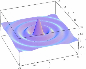
Figure 1. ρ from Equation (5) with $A_{0}=\frac{1}{2}$
, ω = 1 and cs
= 1 at t = 0 (units are arbitrary).
$A_{0}=\frac{1}{2}$
, ω = 1 and cs
= 1 at t = 0 (units are arbitrary).
Standing spherical waves do have a notion of localization. The point o where the amplitude A(r) reaches its global maximum is called the wave center, which is in the case of the above example the origin. It is one of the key parameters for a description of the standing spherical wave, complemented by the frequency ω. Since there is only one single frequency ω involved, this is a monochromatic phenomenon.
With the speed of sound, cs , being the limiting speed of the medium, and setting
 \begin{equation}
\gamma _s \eqcellsep = \eqcellsep \sqrt{1-\frac{v^{2}}{c_s^{2}}},\\
\end{equation}
\begin{equation}
\gamma _s \eqcellsep = \eqcellsep \sqrt{1-\frac{v^{2}}{c_s^{2}}},\\
\end{equation}
 \begin{equation}
t^{\prime } \eqcellsep = \eqcellsep \frac{1}{\gamma _s}\left(t-\frac{v}{c_s^{2}}z\right),\\
\end{equation}
\begin{equation}
t^{\prime } \eqcellsep = \eqcellsep \frac{1}{\gamma _s}\left(t-\frac{v}{c_s^{2}}z\right),\\
\end{equation}
 \begin{equation}
z^{\prime } \eqcellsep = \eqcellsep \frac{1}{\gamma _s}(z-vt),\\
\end{equation}
\begin{equation}
z^{\prime } \eqcellsep = \eqcellsep \frac{1}{\gamma _s}(z-vt),\\
\end{equation}
 \begin{equation}
r^{\prime } \eqcellsep = \eqcellsep \left(x^{2}+y^{2}+z^{\prime 2}\right)^{\frac{1}{2}},
\end{equation}
\begin{equation}
r^{\prime } \eqcellsep = \eqcellsep \left(x^{2}+y^{2}+z^{\prime 2}\right)^{\frac{1}{2}},
\end{equation}
 \begin{equation}
\rho \eqcellsep = \eqcellsep 2A_{0}\frac{{\rm sin} (kr^{\prime })}{r^{\prime }}{\rm cos} (\omega t^{\prime }),\\
\end{equation}
\begin{equation}
\rho \eqcellsep = \eqcellsep 2A_{0}\frac{{\rm sin} (kr^{\prime })}{r^{\prime }}{\rm cos} (\omega t^{\prime }),\\
\end{equation}
 \begin{equation}
\eqcellsep = \eqcellsep A(r^{\prime }) B(t^{\prime })
\end{equation}
\begin{equation}
\eqcellsep = \eqcellsep A(r^{\prime }) B(t^{\prime })
\end{equation}
Equations (7)– (9) are close to the formulas for the Lorentz transformation used in relativity and the use of these formulas within classical mechanics is unusual. We note explicitly here that this has nothing to do with the theory of Special Relativity, but merely constitutes the mathematical description of propagating spherons, which are physical solutions of the classical wave equation. An explicit calculation quickly shows that Equation (12) solves the wave equation whereas the use of quantities resulting from a Galilean transformation in Equation (6) does not result in such a solution. Mathematically this will not come as a surprise, since the wave equation is known as an invariant of the Lorentz transformation and it is not an invariant of the Galilean transformation.
Equations (7)– (9) should therefore be thought of as a “Lorentz composition of quantities” instead of a Lorentz transformation in order to avoid confusion with relativistic ideas and terminology. So while the use of such a Lorentz composition is commanded by the wave-nature of spherons, we have defined our factor γ s not in the usual way used in Special Relativity (the usual notation applied there is γ = 1/γ s ) to remind us of the fact that we are not explicitly dealing with Special Relativity here. Instead, the idealised universe is based on classical mechanics in classical space and time.
We now populate this universe with matter. To represent matter without rest mass (radiation) we choose moving plane waves that follow Equation (2). Such waves transport energy at the speed of sound and cannot stand still. We choose spherons to represent matter with rest mass. Our choice is justified by the similarities between the properties of spherons in the idealised universe and the properties of matter with rest mass in our real universe, which are laid out in the next section. From these elementary particles we envision more complex material entities being built, including intelligent beings that are able to observe their environment and perform measurements with their material tools, all of which are composed of elementary particles which are spherons in the idealised universe. We call such an intelligent being a “spheronic observer”.
For the sake of the present argument we ignore the fact that the spherons cannot interact. This is due to the linearity which is a consequence of the assumptions made and is addressed later. We reiterate that the idealised universe is filled with spherons which are its elementary particles with rest mass. The gas is merely a (hypothetical) medium which aids our discussion and which sustains the existence of the spherons. Observers made of spheronic “matter” cannot detect this gas as explained in the next section.
3 SPHERONS
The wave center of Equation (12) is moving with speed v in the z-direction as can be seen by setting z′ = 0 and solving for z. So compared to a standing spherical wave, a spheron naturally needs the velocity vector v as an additional parameter for its description. Equation (12) also shows that a spheron may be understood to be composed of two parts: The amplitude A(r ′) and an oscillating part B(t ′).
From the transformation it is evident that the speed of sound is the limiting speed for the spheron. Physically, this will come as no surprise, since the speed of sound is the limiting speed of energy transport in the medium and a propagating spheron is “transporting” energy.
Note that an observer consisting of spherons does not experience a resistance from the medium while moving. There is no “airflow” around a spheron because spherons propagate as waves and are not solid bodies moving through the medium.
3.1 Length contraction and time dilation
A spheronic observer has no ab-initio knowledge of space-time and has to derive measurement rods and clocks from the properties of spheronic matter.
To define the rods of a comoving spheronic observer, let his or her defining standard ruler stretch from the wave center to the first zero of the amplitude A(r ′). While this delivers the desired length scales derived from the properties of a spheron, the standard ruler should not be thought of as a thing made of “solid real” matter. It remains a wave-natured measurement tool and for a spheronic observer a measurement is a process determined by the properties of his or her tools
Every existing real clock relies on the counting of some cyclic event provided by the matter the clock is made of. To define a spheronic clock, let the observer count the oscillations in the wave center. This wrist watch then defines his/her proper time.
The effect of the Lorentz-composition on the amplitude A(r ′) is shown in Figure 2. Compared to Figure 1, the waves centered around the wave center in Figure 1 have acquired an elliptic shape. This is a “relativistic” contraction in direction of propagation. The quotes are meant to indicate once more that this “relativistic” contraction is based on the speed of sound as the limiting speed, and not on the speed of light in our real universe. From here on, we assume that the reader keeps this in mind and leave the quotes away for ease of reading. Besides this difference in limiting speeds, the effect follows the pattern of a contraction in Special Relativity in the real universe, which is a consequence of the formulas used.


Writing out B(t′) = cos(ω t′)
 \begin{equation}
B(t) = {\rm cos}\left(\frac{\omega }{\gamma _s}\left(t-\frac{v}{c_s^{2}}z\right)\right),
\end{equation}
\begin{equation}
B(t) = {\rm cos}\left(\frac{\omega }{\gamma _s}\left(t-\frac{v}{c_s^{2}}z\right)\right),
\end{equation}
and for a virtual (spheronic) observer at rest, say at z = 0, the frequency becomes
 \begin{equation}
B(t^{^{\prime }}\left(z=0\right))={\rm cos}\left(\frac{\omega }{\gamma _s}\left(t\right)\right),\vspace*{-4pt}
\end{equation}
\begin{equation}
B(t^{^{\prime }}\left(z=0\right))={\rm cos}\left(\frac{\omega }{\gamma _s}\left(t\right)\right),\vspace*{-4pt}
\end{equation}
and thus ω′ = ω/γ s > ω. The term
 \begin{equation}
\omega ^{\prime }=\frac{\omega }{\sqrt{1-\frac{v^{2}}{c_s^{2}}}}, \vspace*{-4pt}
\end{equation}
\begin{equation}
\omega ^{\prime }=\frac{\omega }{\sqrt{1-\frac{v^{2}}{c_s^{2}}}}, \vspace*{-4pt}
\end{equation}
resembles, in the real universe, the mass term,
 \begin{equation}
m=\frac{m_{0}}{\sqrt{1-\frac{v^{2}}{c^{2}}}},
\end{equation}
\begin{equation}
m=\frac{m_{0}}{\sqrt{1-\frac{v^{2}}{c^{2}}}},
\end{equation}
of special relativity, where m 0 is the rest mass.
In the idealised universe, for a virtual spheronic observer comoving with the wave center, z = vt, and thus the oscillation is
 \begin{equation}
B\left(t^{^{\prime }}\left(z=vt\right)\right) \eqcellsep = \eqcellsep {\rm cos}\left(\frac{\omega }{\gamma _s}\left(t-\frac{v}{c^{2}}vt\right)\right),\\
\end{equation}
\begin{equation}
B\left(t^{^{\prime }}\left(z=vt\right)\right) \eqcellsep = \eqcellsep {\rm cos}\left(\frac{\omega }{\gamma _s}\left(t-\frac{v}{c^{2}}vt\right)\right),\\
\end{equation}
 \begin{equation}
\eqcellsep = \eqcellsep {\rm cos}\left(\gamma _s\omega t\right),
\end{equation}
\begin{equation}
\eqcellsep = \eqcellsep {\rm cos}\left(\gamma _s\omega t\right),
\end{equation}
3.2 Phase waves and operator methods
The wave part of the spheron at rest is a harmonic oscillation. The wave part of a propagating spheron (Equation (13)) is a moving plane wave with phase velocity
 \begin{equation}
v_{P}=\frac{c_s}{v}c_s,
\end{equation}
\begin{equation}
v_{P}=\frac{c_s}{v}c_s,
\end{equation}
as can be seen from setting t − vz/c 2 s = 0 and solving for z. The speed of the phase is larger by a factor cs /v than the speed of sound. This supersonic phase speed resembles the superluminal phase speed of a quantum mechanical de Broglie wave. The phase speed does not interfere with the speed of sound as the limiting speed of energy transport in the medium, since this phase wave does not transport any energy. The same applies to a de Broglie wave. Also Equations (14) and (18) may be seen as a “theorem of phase harmony” (“théorème de l’harmonie de phases”, de Broglie 1925) in action.
The plane wave described by Equation (13) is in many respects a “phase wave” as is the original “onde de phase” of de Broglie and could therefore be termed a “real de Broglie wave”. Figure 3 shows a moving spheron as the multiplication of a contracted amplitude with a plane phase wave.
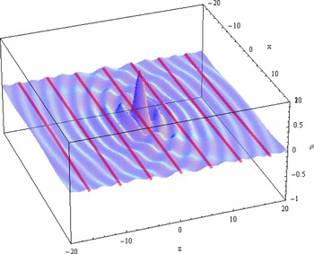
Figure 3. As Figure 2. Spheron with $A_{0}=\frac{1}{2}$
, ω = 1, cs
= 1 and v = 0.75cs
. The wavefronts of the phase wave are marked in red.
$A_{0}=\frac{1}{2}$
, ω = 1, cs
= 1 and v = 0.75cs
. The wavefronts of the phase wave are marked in red.
It is common practice to employ complex quantities (see e.g. Skudrzyk 1971) for the description of plane waves, since that simplifies the calculations considerably. The phase wave of a propagating spheron may be written in complex notation as e iωt′. For velocities small compared to the speed of sound, v ≪ cs , an approximation may be used. Using the identities
 \begin{equation}
\frac{\partial }{\partial t}e^{i\omega t^{\prime }} \eqcellsep \equiv \eqcellsep i\frac{\omega }{\gamma _s}e^{i\omega t^{\prime }},\\
\end{equation}
\begin{equation}
\frac{\partial }{\partial t}e^{i\omega t^{\prime }} \eqcellsep \equiv \eqcellsep i\frac{\omega }{\gamma _s}e^{i\omega t^{\prime }},\\
\end{equation}
 \begin{equation}
\nabla ^{2}e^{i\omega t^{\prime }} \eqcellsep \equiv \eqcellsep \left(i\frac{\omega }{\gamma _s}\frac{\mathbf {v}}{c_s^{2}}\right)^{2}e^{i\omega t^{\prime }},
\end{equation}
\begin{equation}
\nabla ^{2}e^{i\omega t^{\prime }} \eqcellsep \equiv \eqcellsep \left(i\frac{\omega }{\gamma _s}\frac{\mathbf {v}}{c_s^{2}}\right)^{2}e^{i\omega t^{\prime }},
\end{equation}
 \begin{equation}
\frac{\omega }{\gamma _s}\approx \omega \left(1+\frac{1}{2}\frac{v^{2}}{c_s^{2}}\right),
\end{equation}
\begin{equation}
\frac{\omega }{\gamma _s}\approx \omega \left(1+\frac{1}{2}\frac{v^{2}}{c_s^{2}}\right),
\end{equation}
and it follows that
 \begin{equation}
\frac{\partial }{\partial t} e^{i\omega t^{\prime }} \eqcellsep \approx \eqcellsep i\omega \left(1+\frac{1}{2}\frac{v^{2}}{c_s^{2}}\right)e^{i\omega t^{\prime }},\\
\end{equation}
\begin{equation}
\frac{\partial }{\partial t} e^{i\omega t^{\prime }} \eqcellsep \approx \eqcellsep i\omega \left(1+\frac{1}{2}\frac{v^{2}}{c_s^{2}}\right)e^{i\omega t^{\prime }},\\
\end{equation}
 \begin{equation}
\nabla ^{2}e^{i\omega t^{\prime }} \eqcellsep \approx \eqcellsep -\omega ^{2}\frac{v^{2}}{c_s^{4}}e^{i\omega t^{\prime }},
\end{equation}
\begin{equation}
\nabla ^{2}e^{i\omega t^{\prime }} \eqcellsep \approx \eqcellsep -\omega ^{2}\frac{v^{2}}{c_s^{4}}e^{i\omega t^{\prime }},
\end{equation}
 \begin{equation}
-i\frac{\partial }{\partial t} e^{i\omega t^{\prime }} = \omega e^{i\omega t^{\prime }}-\frac{c_s^{2}\nabla ^{2}e^{i\omega t^{\prime }}}{2\omega }
\end{equation}
\begin{equation}
-i\frac{\partial }{\partial t} e^{i\omega t^{\prime }} = \omega e^{i\omega t^{\prime }}-\frac{c_s^{2}\nabla ^{2}e^{i\omega t^{\prime }}}{2\omega }
\end{equation}
can be concluded. Remarkably, this resembles a “Schrödinger-Equation” for an unbound particle. Slowly (v ≪ cs ) moving elementary particles of the idealised universe, slow spherons, thus obey a Schrödinger-like equation. Also, for purely algebraical reasons, this phase wave is a solution of a “Klein-Gordon-Equation”, where the frequency ω plays the role of the mass in the real Klein-Gordon equation,
 \begin{equation}
\left(\frac{1}{c_s^{2}}\frac{\partial ^{2}}{\partial t^{2}}-\nabla ^{2}\right)e^{i\omega t^{\prime }}=-\frac{\omega ^{2}}{c_s^{2}}e^{i\omega t^{\prime }}.
\end{equation}
\begin{equation}
\left(\frac{1}{c_s^{2}}\frac{\partial ^{2}}{\partial t^{2}}-\nabla ^{2}\right)e^{i\omega t^{\prime }}=-\frac{\omega ^{2}}{c_s^{2}}e^{i\omega t^{\prime }}.
\end{equation}
All this makes it tempting to explore the applicability of other quantum mechanical mathematics to spherons.
Written in complex notation, Equation (11) becomes
 \begin{equation}
\rho =2A_{0}\frac{{\rm sin}\left(kr^{\prime }\right)}{r^{\prime }}e^{i\omega t^{\prime }},
\end{equation}
\begin{equation}
\rho =2A_{0}\frac{{\rm sin}\left(kr^{\prime }\right)}{r^{\prime }}e^{i\omega t^{\prime }},
\end{equation}
and
 \begin{equation}
\rho ^{*}=2A_{0}\frac{{\rm sin}\left(kr^{\prime }\right)}{r^{\prime }}e^{-i\omega t^{\prime }}
\end{equation}
\begin{equation}
\rho ^{*}=2A_{0}\frac{{\rm sin}\left(kr^{\prime }\right)}{r^{\prime }}e^{-i\omega t^{\prime }}
\end{equation}
is its complex conjugate. Accordingly,
 \begin{equation}
\rho \rho ^{*}=\left(2A_{0}\frac{{\rm sin}\left(kr^{\prime }\right)}{r^{\prime }}\right)^{2},
\end{equation}
\begin{equation}
\rho \rho ^{*}=\left(2A_{0}\frac{{\rm sin}\left(kr^{\prime }\right)}{r^{\prime }}\right)^{2},
\end{equation}
since e iωt′ e − iωt′ = 1 always holds. The volume integral over ρρ* is
 \begin{equation}
\int \rho \rho ^{*}dV = 4A_{0}^{2}2\pi 2\gamma _s\left[\frac{1}{2}r^{\prime }-\frac{1}{4k}{\rm sin}\left(2kr^{\prime }\right)\right]_{0}^{R^{\prime }}
\end{equation}
\begin{equation}
\int \rho \rho ^{*}dV = 4A_{0}^{2}2\pi 2\gamma _s\left[\frac{1}{2}r^{\prime }-\frac{1}{4k}{\rm sin}\left(2kr^{\prime }\right)\right]_{0}^{R^{\prime }}
\end{equation}
(see Appendix B), where R′ is the radius associated with the volume V. The integral is not a constant value. To enforce a value of 1 for the volume integral, a factor
 \begin{equation}
\vartheta ^{\prime }=\frac{1}{2A_{0}}\frac{1}{\pi r^{\prime }}\sqrt{\frac{1}{2k\gamma _s}}
\end{equation}
\begin{equation}
\vartheta ^{\prime }=\frac{1}{2A_{0}}\frac{1}{\pi r^{\prime }}\sqrt{\frac{1}{2k\gamma _s}}
\end{equation}
may be used (see Appendix B). Setting
 \begin{equation}
\chi \eqcellsep = \eqcellsep \vartheta ^{\prime } 2A_{0}\frac{{\rm sin}\left(kr^{\prime }\right)}{r^{\prime }},\\
\end{equation}
\begin{equation}
\chi \eqcellsep = \eqcellsep \vartheta ^{\prime } 2A_{0}\frac{{\rm sin}\left(kr^{\prime }\right)}{r^{\prime }},\\
\end{equation}
 \begin{equation}
\eqcellsep = \eqcellsep \frac{1}{\pi r^{\prime }}\sqrt{\frac{1}{2k\gamma _s}}\frac{{\rm sin}\left(kr^{\prime }\right)}{r^{\prime }},
\end{equation}
\begin{equation}
\eqcellsep = \eqcellsep \frac{1}{\pi r^{\prime }}\sqrt{\frac{1}{2k\gamma _s}}\frac{{\rm sin}\left(kr^{\prime }\right)}{r^{\prime }},
\end{equation}
 \begin{equation}
\psi =\chi e^{i\omega t},
\end{equation}
\begin{equation}
\psi =\chi e^{i\omega t},
\end{equation}
leads to
 \begin{equation}
\int \psi ^{*}\psi dV=\int \chi ^{2}dV=1.
\end{equation}
\begin{equation}
\int \psi ^{*}\psi dV=\int \chi ^{2}dV=1.
\end{equation}
The quantity ψ may be seen as representing physical quantities of Equation (12), since it allows for a recovery of elementary properties of the spheron with operator-methods in the following way (for a detailed calculation, see Appendix B): Define
 \begin{equation}
\mathbf {\hat{x}}=x\, \mathbf {e_{x}}+y\, \mathbf {e_{y}}+z\, \mathbf {e_{z}},
\end{equation}
\begin{equation}
\mathbf {\hat{x}}=x\, \mathbf {e_{x}}+y\, \mathbf {e_{y}}+z\, \mathbf {e_{z}},
\end{equation}
then the wave-center of the spheron can be recovered with
 \begin{equation}
\mathbf {o}=\int \psi ^{*} \, \mathbf {\hat{x}} \,\psi \, dV,
\end{equation}
\begin{equation}
\mathbf {o}=\int \psi ^{*} \, \mathbf {\hat{x}} \,\psi \, dV,
\end{equation}
a quantity depending on the frequency is delivered by
 \begin{equation}
\frac{\omega }{\gamma _s} = \int \psi ^{*}\left(-i\frac{\partial }{\partial t}\right)\psi \, dV
\end{equation}
\begin{equation}
\frac{\omega }{\gamma _s} = \int \psi ^{*}\left(-i\frac{\partial }{\partial t}\right)\psi \, dV
\end{equation}
and a quantity depending on the velocity is obtained with
 \begin{equation}
\frac{\omega }{\gamma _s}\frac{\mathrm{1}}{c_s^{2}}\mathbf {v}=\int \psi ^{*} \, i \, \mathbf {\nabla } \, \psi \,dV.
\end{equation}
\begin{equation}
\frac{\omega }{\gamma _s}\frac{\mathrm{1}}{c_s^{2}}\mathbf {v}=\int \psi ^{*} \, i \, \mathbf {\nabla } \, \psi \,dV.
\end{equation}
These operators are close to the quantum-mechanical operators for location, energy and momentum respectively.
Other analogies can be found, but discussing them here will not add any more insight concerning the subject of this contribution. Nevertheless one last remark is in order: since the wave equation results from applying classical mechanics to the medium, it is perfectly possible to employ Hamiltonians or Lagrangians, as is common practice in quantum mechanics.
3.3 A spheronic theory of relativity
The Lorentz composition results in relativistic effects for the amplitude and quantum mechanical effects for the wave part at the same time. The spheron can only be fully understood by considering both aspects at the same time, it is a phase wave and a “localised” amplitude represented by a point-like wave center, one entity with a “dualistic” nature. This concludes our reasoning for choosing spherons as representing matter with rest mass in our toy universe.
Contraction and dilation provide a direct path to special relativity, including the 4-dimensional space-time, and the full apparatus of relativity. To get there, it is necessary to give up the human perspective and adopt the perspective of a spheronic observer.
First we note that a spheronic observer has no means to measure his state of motion against the gas. If he would construct a “spheronic interferometer” to measure his/her speed against a hypothesised “ether”, he would end up with a null-result, as did Michelson and Morley with their experiments to measure an ether drift in the late 19th century. This can be shown by an explicit calculation, but it is easier to remind oneself that the only reason to introduce the contraction of rods and the dilation of clocks were the need to explain these unexpected null-results.
With the ideas of rigid bodies in mind, these indeed seem to be awkward ad-hoc explanations with little physical plausibility. In his 1908 paper, Minkowski acknowledges them to work mathematically but calls them a “present from above” (“Geschenk von oben”, Minkowski 1908). He then states that Lorentz’ idea is completely equivalent (“völlig äquivalent”) to his new conception of time and space.
From the perspective of a human physicist, an analogue to a Lorentzian ether theory is the best choice to describe the vibrations of the medium. Note, that the relativistic contraction and dilation in the idealised universe are no “present from above”, but a direct consequence of the wave nature (“Wellenartigkeit”) of matter.
From the perspective of an internal spheronic observer, things are different. What is an obvious and measurable contraction of the spheronic observer’s standard ruler for an external human (who is not an observer made of spheronic matter and who therefore can observe the idealised universe from “outside” by not being part of it) is actually unmeasurable and unnoticeable to the spheronic observerFootnote 1 . The same applies to the dilation of proper time. The spheronic observer’s standard ruler and clock define her/his units of measurement. Putting oneself in the position of such an observer with the task of developing a physical theory leads to a spheronic theory of relativity.
A human observer in the real universe thinking up the idealised universe can easily switch between these two perspectives. This makes it possible to explore all the seemingly paradoxical results of relativity within the classical framework of our idealised universe. This includes, among other issues, the relativity of simultaneity and the twin paradox. With a set of comoving synchronised spheronical co-observers it is also possible to setup a 4-dimensional spheronic space-time on that basis.
Beyond that it might be interesting to note that the intimate relation between time and space measured and experienced by a spheronic observer is deeply rooted in the material (i.e. spheronic) nature of her/his existence. It is for this reason, that a spheronic observer always measures the speed of sound to be a constant quantity.
But the properties of the matter the observer is made of determine the reality of a spheronic observer to an even greater extent. The material layer effectively shields a spheronic observer from the underlying physical reality and cannot be circumvented by him. As a result e.g. the existence of the full fledged wave function is, for a spheronic observer, not measurable and remains a non-physical (sub- trans- or meta-physical) speculation for him. The reach of her/his material tools define the reach of her/his physical theories.
4 DISCUSSION
The gedanken experiment presented here, in which an idealised universe is created from simple classical principles, indicates intriguing properties that resemble some important aspects of our real world. These aspects may be relevant for a quantum mechanical and special relativistic understanding of our real universe.
In our real universe, we are in a position which is in many respects similar to the situation of spheronic observers in the idealised universe. Like them we are made of matter which can be described as waves, and such are all our tools and means to gather information about the universe we inhabit.
Turning back to our idealised world, we have thus discovered that the very simple approach of analyzing a known solution of the wave equation with tools usually not applied there can reveal many elements of modern physics. Among these are a natural speed limit for entities, relativistic contraction and time dilation as well as supersonic (superluminal) phase waves and an example how a “ridiculous looking proposal” (Penrose 2005, page 500) of an operator-logic can be founded in geometrical properties of the object under study.
The reader will have noticed a major difference between a “de Broglie wave” associated to a spheron and the de Broglie wave associated with a particle in traditional quantum mechanics. Following a paradigm already present in de Broglie’s nobel-prize winning thesis, traditional quantum mechanical models treat a particle as a wave-packet to arrive at a localised entity. This packet is made of a continuous spectrum of de Broglie waves and although there cannot be any experimental evidence for this it still seems to be the standard model (e.g. Tipler & Llewellyn 2002). Within this scheme, quantum mechanics needs to postulate for every class of elementary particle a separate field. In contrast to this, a spheron is localised by its amplitude, which is “associated” to the “de Broglie wave” by multiplication. As a consequence of this, our idealised quantum mechanics needs just one “field” with just one governing “universal” equation and the various types of particles are modelled as different solutions to this. In the case of the spheron, the amplitude complements the “de Broglie wave” and both together solve the wave equation, while the “de Broglie wave” only solves the “Klein-Gordon-equation”.
Naturally, we emphasised more the similarities than the differences between spherons and matter, of which there are plenty. To mention only one: Spherons do not interact with any other vibrations, be it another spheron or a plane wave. This is due to the linearity of the wave equation which leads to the possibility of superimposing solutions to generate a new one. Other properties of real matter are missing completely. In the real universe, there is definitely more than one type of elementary particle and there are properties like spin, which have no counterpart in spherons.
Some of these differences might be studied within the framework of the idealised universe by varying the properties of the medium, since this generally determines the existence, the properties of and the interaction between the wave solutions that can exist within it. Giving up on the linearity of the wave equation means giving up the superposition principle and would thus enforce interacting entities. Keeping the linearity but dropping the requirement of a curl-free medium allows for it to harbor more diverse classes of vibrations including phenomena with spin-like properties.
It is generally an interesting endeavor to hunt for analogies and various more or less obvious possibilities to do so provide a vast playground. Whatever the odds are to develop a model that comes closer to observed reality: it seems remarkable that even such a most simple medium as an idealised gas can reproduce so much of the fundamental elements of modern physics.
Our gedanken experiment may thus shed an interesting light on interpreting the quantum mechanical and special relativistic properties of the real universe, in the sense that these two properties may be two sides of the same coin. But, perhaps more importantly, the present spheron-gedanken experiment may be useful for teaching quantum mechanics and special relativity, as a means of visualizing the possibly intimate connection between the wave-like properties of matter and special relativity, in the sense that if real matter can be described by waves then special relativity automatically emerges.
ACKNOWLEDGEMENTS
We thank the referee for very careful analysis of the material presented here and for helpful suggestions which clarified the arguments. The challenge discussed in Appendix C has been posed by the referee.
APPENDIX A REAL DE-BROGLIE WAVES
To make the relationship between the wave part of a moving spheron in our idealised universe and a quantum-mechanical de Broglie wave in the real universe (in which the limiting speed is the speed of light, c) explicit, note that a de Broglie wave in the real universe associated with a particle of rest mass m 0, moving in the direction of increasing values of z, is usually written as
 \begin{equation}
B\left(x,t\right)=e^{i\left(pz-Et\right)/\hbar },
\end{equation}
\begin{equation}
B\left(x,t\right)=e^{i\left(pz-Et\right)/\hbar },
\end{equation}
where E = ℏw is the relativistic energy and p = ℏk is the relativistic momentum. The energy is
 \begin{equation}
E \eqcellsep = \eqcellsep mc^{2}=\hbar w,\\
\end{equation}
\begin{equation}
E \eqcellsep = \eqcellsep mc^{2}=\hbar w,\\
\end{equation}
 \begin{equation}
\eqcellsep = \eqcellsep \frac{m_{0}}{\sqrt{1-\frac{v^{2}}{c^{2}}}}c^{2}=\hbar \frac{w_{0}}{\sqrt{1-\frac{v^{2}}{c^{2}}}},
\end{equation}
\begin{equation}
\eqcellsep = \eqcellsep \frac{m_{0}}{\sqrt{1-\frac{v^{2}}{c^{2}}}}c^{2}=\hbar \frac{w_{0}}{\sqrt{1-\frac{v^{2}}{c^{2}}}},
\end{equation}
 \begin{equation}
p \eqcellsep = \eqcellsep mv=\frac{E}{c^{2}}v=\hbar k,\\
\end{equation}
\begin{equation}
p \eqcellsep = \eqcellsep mv=\frac{E}{c^{2}}v=\hbar k,\\
\end{equation}
 \begin{equation}
\eqcellsep = \eqcellsep \frac{m_{0}}{\sqrt{1-\frac{v^{2}}{c^{2}}}}v=\hbar \frac{w_{0}}{\sqrt{1-\frac{v^{2}}{c^{2}}}}\frac{1}{c^{2}}v=\hbar k.
\end{equation}
\begin{equation}
\eqcellsep = \eqcellsep \frac{m_{0}}{\sqrt{1-\frac{v^{2}}{c^{2}}}}v=\hbar \frac{w_{0}}{\sqrt{1-\frac{v^{2}}{c^{2}}}}\frac{1}{c^{2}}v=\hbar k.
\end{equation}
 \begin{equation}
Et-pz \eqcellsep = \eqcellsep \hbar \frac{w_{0}}{\sqrt{1-\frac{v^{2}}{c^{2}}}}t-\hbar \frac{v}{c^{2}}\frac{w_{0}}{\sqrt{1-\frac{v^{2}}{c^{2}}}}z,\\
\end{equation}
\begin{equation}
Et-pz \eqcellsep = \eqcellsep \hbar \frac{w_{0}}{\sqrt{1-\frac{v^{2}}{c^{2}}}}t-\hbar \frac{v}{c^{2}}\frac{w_{0}}{\sqrt{1-\frac{v^{2}}{c^{2}}}}z,\\
\end{equation}
 \begin{equation}
\eqcellsep = \eqcellsep \hbar \frac{w_{0}}{\sqrt{1-\frac{v^{2}}{c^{2}}}}\left(t-\frac{v}{c^{2}}z\right).
\end{equation}
\begin{equation}
\eqcellsep = \eqcellsep \hbar \frac{w_{0}}{\sqrt{1-\frac{v^{2}}{c^{2}}}}\left(t-\frac{v}{c^{2}}z\right).
\end{equation}
 \begin{equation}
B\left(x,t\right) \eqcellsep = \eqcellsep e^{-i\left(\frac{w_{0}}{\gamma _s}\left(t-\frac{v}{c^{2}}z\right)\right)},\\
\end{equation}
\begin{equation}
B\left(x,t\right) \eqcellsep = \eqcellsep e^{-i\left(\frac{w_{0}}{\gamma _s}\left(t-\frac{v}{c^{2}}z\right)\right)},\\
\end{equation}
 \begin{equation}
\eqcellsep = \eqcellsep e^{-i\left(w_{0}t\mbox{'}\right)},\\
\end{equation}
\begin{equation}
\eqcellsep = \eqcellsep e^{-i\left(w_{0}t\mbox{'}\right)},\\
\end{equation}
 \begin{equation}
\eqcellsep = \eqcellsep {\rm cos}\left(-w_{0}t\mbox{'}\right)+i\, {\rm sin}\left(-w_{0}t\mbox{'}\right),
\end{equation}
\begin{equation}
\eqcellsep = \eqcellsep {\rm cos}\left(-w_{0}t\mbox{'}\right)+i\, {\rm sin}\left(-w_{0}t\mbox{'}\right),
\end{equation}
 \begin{equation}
B\left(t^{\prime }\right)={\rm cos}\left(\omega t^{\prime }\right),
\end{equation}
\begin{equation}
B\left(t^{\prime }\right)={\rm cos}\left(\omega t^{\prime }\right),
\end{equation}
(see eqs 11 and 12), which is the plane wave part of the moving spheron. Since cos(− α) = cos(α) (A11) may thus be seen as the real part of a de Broglie type plane wave.
APPENDIX B VOLUME INTEGRALS AND OPERATORS
Based on (eqs 7-10) and assuming there is a speed limit c (which is cs in our idealised universe or the speed of light in the real universe)
 \begin{equation}
r^{\prime } \eqcellsep = \eqcellsep \big(x^{2}+y^{2}+z^{^{\prime 2}}\big)^{\frac{1}{2}},\\
\end{equation}
\begin{equation}
r^{\prime } \eqcellsep = \eqcellsep \big(x^{2}+y^{2}+z^{^{\prime 2}}\big)^{\frac{1}{2}},\\
\end{equation}
 \begin{equation}
\eqcellsep = \eqcellsep r\left(1+\frac{z^{^{\prime 2}}-z^{2}}{r^{2}}\right)^{\frac{1}{2}},\\
\end{equation}
\begin{equation}
\eqcellsep = \eqcellsep r\left(1+\frac{z^{^{\prime 2}}-z^{2}}{r^{2}}\right)^{\frac{1}{2}},\\
\end{equation}
 \begin{equation}
\eqcellsep = \eqcellsep r\left(1+\frac{\frac{\left(z-vt\right)^{2}}{1-\frac{v^{2}}{c^{2}}}-z^{2}}{r^{2}}\right)^{\frac{1}{2}},
\end{equation}
\begin{equation}
\eqcellsep = \eqcellsep r\left(1+\frac{\frac{\left(z-vt\right)^{2}}{1-\frac{v^{2}}{c^{2}}}-z^{2}}{r^{2}}\right)^{\frac{1}{2}},
\end{equation}
 \begin{equation}
r^{\prime } \eqcellsep = \eqcellsep r\left(1+\frac{\frac{z^{2}}{1-\frac{v^{2}}{c^{2}}}-z^{2}}{r^{2}}\right)^{\frac{1}{2}},\\
\end{equation}
\begin{equation}
r^{\prime } \eqcellsep = \eqcellsep r\left(1+\frac{\frac{z^{2}}{1-\frac{v^{2}}{c^{2}}}-z^{2}}{r^{2}}\right)^{\frac{1}{2}},\\
\end{equation}
 \begin{equation}
\eqcellsep = \eqcellsep r\left(1+\frac{\frac{1-\left(1-\frac{v^{2}}{c^{2}}\right)}{1-\frac{v^{2}}{c^{2}}}z^{2}}{r^{2}}\right)^{\frac{1}{2}},
\end{equation}
\begin{equation}
\eqcellsep = \eqcellsep r\left(1+\frac{\frac{1-\left(1-\frac{v^{2}}{c^{2}}\right)}{1-\frac{v^{2}}{c^{2}}}z^{2}}{r^{2}}\right)^{\frac{1}{2}},
\end{equation}
 \begin{equation}
{\rm cos}\left(\theta \right)=\frac{z}{r},
\end{equation}
\begin{equation}
{\rm cos}\left(\theta \right)=\frac{z}{r},
\end{equation}
this may be written as
 \begin{equation}
r^{\prime }=r\left(1+\left(\frac{1-\gamma _s^{2}}{\gamma _s^{2}}\right){\rm cos}^{2}\left(\theta \right)\right)^{\frac{1}{2}}.
\end{equation}
\begin{equation}
r^{\prime }=r\left(1+\left(\frac{1-\gamma _s^{2}}{\gamma _s^{2}}\right){\rm cos}^{2}\left(\theta \right)\right)^{\frac{1}{2}}.
\end{equation}
Therefore
 \begin{equation}
dr^{\prime }=dr\left(1+\left(\frac{1-\gamma _s^{2}}{\gamma _s^{2}}\right){\rm cos}^{2}\left(\theta \right)\right)^{\frac{1}{2}},
\end{equation}
\begin{equation}
dr^{\prime }=dr\left(1+\left(\frac{1-\gamma _s^{2}}{\gamma _s^{2}}\right){\rm cos}^{2}\left(\theta \right)\right)^{\frac{1}{2}},
\end{equation}
or
 \begin{equation}
r \eqcellsep = \eqcellsep \frac{r^{\prime }}{\left(1+\left(\frac{1-\gamma _s^{2}}{\gamma _s^{2}}\right){\rm cos}^{2}\left(\theta \right)\right)^{\frac{1}{2}}},\\
\end{equation}
\begin{equation}
r \eqcellsep = \eqcellsep \frac{r^{\prime }}{\left(1+\left(\frac{1-\gamma _s^{2}}{\gamma _s^{2}}\right){\rm cos}^{2}\left(\theta \right)\right)^{\frac{1}{2}}},\\
\end{equation}
 \begin{equation}
dr \eqcellsep = \eqcellsep \frac{dr^{\prime }}{\left(1+\left(\frac{1-\gamma _s^{2}}{\gamma _s^{2}}\right){\rm cos}^{2}\left(\theta \right)\right)^{\frac{1}{2}}},
\end{equation}
\begin{equation}
dr \eqcellsep = \eqcellsep \frac{dr^{\prime }}{\left(1+\left(\frac{1-\gamma _s^{2}}{\gamma _s^{2}}\right){\rm cos}^{2}\left(\theta \right)\right)^{\frac{1}{2}}},
\end{equation} $\rho =2A_{0}\frac{{\rm sin}\left(kr^{\prime }\right)}{r^{\prime }}e^{i\omega t^{\prime }}$
, the volume integral over ρρ* is
$\rho =2A_{0}\frac{{\rm sin}\left(kr^{\prime }\right)}{r^{\prime }}e^{i\omega t^{\prime }}$
, the volume integral over ρρ* is
 \begin{equation}
\int \rho \rho ^{*}dV \eqcellsep = \eqcellsep \int \int \int A^{2}\left(r^{\prime }\right)r^{2}{\rm sin}\left(\theta \right)drd\theta d\phi ,\\
\end{equation}
\begin{equation}
\int \rho \rho ^{*}dV \eqcellsep = \eqcellsep \int \int \int A^{2}\left(r^{\prime }\right)r^{2}{\rm sin}\left(\theta \right)drd\theta d\phi ,\\
\end{equation}
 \begin{equation}
\eqcellsep = \eqcellsep \int \int \int A^{2}\left(r^{\prime }\right)\frac{r^{^{\prime 2}}}{\left(1+\left(\frac{1-\gamma _s^{2}}{\gamma _s^{2}}\right){\rm cos}^{2}\left(\theta \right)\right)^{\frac{3}{2}}} \nonumber \\
\eqcellsep \times \eqcellsep {\rm sin}\left(\theta \right)dr^{\prime }d\theta d\phi .
\end{equation}
\begin{equation}
\eqcellsep = \eqcellsep \int \int \int A^{2}\left(r^{\prime }\right)\frac{r^{^{\prime 2}}}{\left(1+\left(\frac{1-\gamma _s^{2}}{\gamma _s^{2}}\right){\rm cos}^{2}\left(\theta \right)\right)^{\frac{3}{2}}} \nonumber \\
\eqcellsep \times \eqcellsep {\rm sin}\left(\theta \right)dr^{\prime }d\theta d\phi .
\end{equation}
 \begin{equation}
\int _{0}^{\pi }\frac{{\rm sin}\left(\theta \right)}{\left(1+\left(\frac{1-\gamma _s^{2}}{\gamma _s^{2}}\right){\rm cos}^{2}\left(\theta \right)\right)^{\frac{3}{2}}}d\theta =\frac{2}{\left(1+\frac{1-\gamma _s^{2}}{\gamma _s^{2}}\right)^{\frac{1}{2}}}=2\gamma _s,
\end{equation}
\begin{equation}
\int _{0}^{\pi }\frac{{\rm sin}\left(\theta \right)}{\left(1+\left(\frac{1-\gamma _s^{2}}{\gamma _s^{2}}\right){\rm cos}^{2}\left(\theta \right)\right)^{\frac{3}{2}}}d\theta =\frac{2}{\left(1+\frac{1-\gamma _s^{2}}{\gamma _s^{2}}\right)^{\frac{1}{2}}}=2\gamma _s,
\end{equation}
and
 \begin{equation}
\int _{0}^{2\pi }d\phi =2\pi ,
\end{equation}
\begin{equation}
\int _{0}^{2\pi }d\phi =2\pi ,
\end{equation}
the volume integral is
 \begin{equation}
\int \rho \rho ^{*}dV \eqcellsep = \eqcellsep 2\gamma _s 2\pi \int A^{2}\left(r^{\prime }\right)r^{^{\prime 2}}dr^{\prime },\\
\end{equation}
\begin{equation}
\int \rho \rho ^{*}dV \eqcellsep = \eqcellsep 2\gamma _s 2\pi \int A^{2}\left(r^{\prime }\right)r^{^{\prime 2}}dr^{\prime },\\
\end{equation}
 \begin{equation}
\eqcellsep = \eqcellsep 2\gamma _s 2\pi \int \left(2A_{0}\frac{{\rm sin}\left(kr^{\prime }\right)}{r^{\prime }}\right)^{2}r^{^{\prime 2}}dr^{\prime },\\
\end{equation}
\begin{equation}
\eqcellsep = \eqcellsep 2\gamma _s 2\pi \int \left(2A_{0}\frac{{\rm sin}\left(kr^{\prime }\right)}{r^{\prime }}\right)^{2}r^{^{\prime 2}}dr^{\prime },\\
\end{equation}
 \begin{equation}
\eqcellsep = \eqcellsep 2\gamma _s 2\pi 4A_{0}^{2}\int {\rm sin}^{2}\left(kr^{\prime }\right)dr^{\prime },\\
\end{equation}
\begin{equation}
\eqcellsep = \eqcellsep 2\gamma _s 2\pi 4A_{0}^{2}\int {\rm sin}^{2}\left(kr^{\prime }\right)dr^{\prime },\\
\end{equation}
 \begin{equation}
\eqcellsep = \eqcellsep 2\gamma _s 2\pi 4A_{0}^{2}\left[\frac{1}{2}r^{\prime }-\frac{1}{4k}{\rm sin}\left(2kr^{\prime }\right)\right]_{0}^{R^{\prime }},
\end{equation}
\begin{equation}
\eqcellsep = \eqcellsep 2\gamma _s 2\pi 4A_{0}^{2}\left[\frac{1}{2}r^{\prime }-\frac{1}{4k}{\rm sin}\left(2kr^{\prime }\right)\right]_{0}^{R^{\prime }},
\end{equation}
 \begin{equation}
\vartheta ^{\prime }=\frac{1}{2A_{0}}\frac{1}{\pi r^{\prime }}\sqrt{\frac{1}{2k\gamma _s}},
\end{equation}
\begin{equation}
\vartheta ^{\prime }=\frac{1}{2A_{0}}\frac{1}{\pi r^{\prime }}\sqrt{\frac{1}{2k\gamma _s}},
\end{equation}
set
 \begin{equation}
\chi \eqcellsep = \eqcellsep\vartheta ^{\prime } 2A_{0}\frac{{\rm sin}\left(kr^{\prime }\right)}{r^{\prime }} = \vartheta ^{\prime } \, A(r^{\prime }),\\
\end{equation}
\begin{equation}
\chi \eqcellsep = \eqcellsep\vartheta ^{\prime } 2A_{0}\frac{{\rm sin}\left(kr^{\prime }\right)}{r^{\prime }} = \vartheta ^{\prime } \, A(r^{\prime }),\\
\end{equation}
 \begin{equation}
\eqcellsep = \eqcellsep \frac{1}{\pi r^{\prime }}\sqrt{\frac{1}{2k\gamma _s}}\frac{{\rm sin}\left(kr^{\prime }\right)}{r^{\prime }},
\end{equation}
\begin{equation}
\eqcellsep = \eqcellsep \frac{1}{\pi r^{\prime }}\sqrt{\frac{1}{2k\gamma _s}}\frac{{\rm sin}\left(kr^{\prime }\right)}{r^{\prime }},
\end{equation}
 \begin{equation*}
\psi =\chi e^{i\omega t},
\end{equation*}
\begin{equation*}
\psi =\chi e^{i\omega t},
\end{equation*}
then
 \begin{equation}
\int \psi ^{*}\psi dV=\int \chi ^{2}dV.
\end{equation}
\begin{equation}
\int \psi ^{*}\psi dV=\int \chi ^{2}dV.
\end{equation}
The volume integral over ψ*ψ is
 \begin{equation}
\int \chi ^{2}dV \eqcellsep = \eqcellsep \int \int \int \left(\frac{1}{\pi r^{\prime }}\sqrt{\frac{1}{2k\gamma _s}}\frac{{\rm sin}\left(kr^{\prime }\right)}{r^{\prime }}\right)^{2}\\
\end{equation}
\begin{equation}
\int \chi ^{2}dV \eqcellsep = \eqcellsep \int \int \int \left(\frac{1}{\pi r^{\prime }}\sqrt{\frac{1}{2k\gamma _s}}\frac{{\rm sin}\left(kr^{\prime }\right)}{r^{\prime }}\right)^{2}\\
\end{equation}
 \begin{equation}
\eqcellsep \times \eqcellsep r^{2}{\rm sin}\left(\theta \right)drd\theta d\phi ,\\
\end{equation}
\begin{equation}
\eqcellsep \times \eqcellsep r^{2}{\rm sin}\left(\theta \right)drd\theta d\phi ,\\
\end{equation}
 \begin{equation}
\eqcellsep = \eqcellsep \frac{1}{\pi ^{2}2k\gamma _s}\int \int \int \left(\frac{1}{r^{\prime }}\frac{{\rm sin}\left(kr^{\prime }\right)}{r^{\prime }}\right)^{2}\\
\end{equation}
\begin{equation}
\eqcellsep = \eqcellsep \frac{1}{\pi ^{2}2k\gamma _s}\int \int \int \left(\frac{1}{r^{\prime }}\frac{{\rm sin}\left(kr^{\prime }\right)}{r^{\prime }}\right)^{2}\\
\end{equation}
 \begin{equation}
\eqcellsep \times \eqcellsep r^{2}{\rm sin}\left(\theta \right)drd\theta d\phi ,\\
\end{equation}
\begin{equation}
\eqcellsep \times \eqcellsep r^{2}{\rm sin}\left(\theta \right)drd\theta d\phi ,\\
\end{equation}
 \begin{equation}
\eqcellsep = \eqcellsep \frac{2\gamma _s 2\pi }{\pi ^{2}2k\gamma _s}\int \left(\frac{1}{r^{\prime }}\frac{{\rm sin}\left(kr^{\prime }\right)}{r^{\prime }}\right)^{2}r^{^{\prime 2}}dr^{\prime },\\
\end{equation}
\begin{equation}
\eqcellsep = \eqcellsep \frac{2\gamma _s 2\pi }{\pi ^{2}2k\gamma _s}\int \left(\frac{1}{r^{\prime }}\frac{{\rm sin}\left(kr^{\prime }\right)}{r^{\prime }}\right)^{2}r^{^{\prime 2}}dr^{\prime },\\
\end{equation}
 \begin{equation}
\eqcellsep = \eqcellsep \frac{2}{\pi k}\int \left(\frac{{\rm sin}\left(kr^{\prime }\right)}{r^{\prime }}\right)^{2}dr^{\prime },\\
\end{equation}
\begin{equation}
\eqcellsep = \eqcellsep \frac{2}{\pi k}\int \left(\frac{{\rm sin}\left(kr^{\prime }\right)}{r^{\prime }}\right)^{2}dr^{\prime },\\
\end{equation}
 \begin{equation}
\eqcellsep = \eqcellsep \frac{2}{k\pi }\left(-\left[\frac{{\rm sin}^{2}\left(kr^{\prime }\right)}{r^{\prime }}\right]_{0}^{R^{\prime }} \right. \\
\end{equation}
\begin{equation}
\eqcellsep = \eqcellsep \frac{2}{k\pi }\left(-\left[\frac{{\rm sin}^{2}\left(kr^{\prime }\right)}{r^{\prime }}\right]_{0}^{R^{\prime }} \right. \\
\end{equation}
 \begin{equation}
\eqcellsep + \eqcellsep \left. k\int _{0}^{R^{\prime }}\frac{{\rm sin}\left(2kr^{\prime }\right)}{r^{\prime }}dr^{\prime }\right).
\end{equation}
\begin{equation}
\eqcellsep + \eqcellsep \left. k\int _{0}^{R^{\prime }}\frac{{\rm sin}\left(2kr^{\prime }\right)}{r^{\prime }}dr^{\prime }\right).
\end{equation}
 \begin{equation}
\int _{r^{\prime }}\left(\frac{{\rm sin}\left(kr^{\prime }\right)}{r^{\prime }}\right)^{2}dr^{\prime },
\end{equation}
\begin{equation}
\int _{r^{\prime }}\left(\frac{{\rm sin}\left(kr^{\prime }\right)}{r^{\prime }}\right)^{2}dr^{\prime },
\end{equation}
thus approaches, for sufficiently large R′ and to arbitrary precision, $k\frac{\pi }{2}$
and the integral of ψ*ψ then comes out as
$k\frac{\pi }{2}$
and the integral of ψ*ψ then comes out as
 \begin{equation}
\int \psi ^{*}\psi \, dV=1.
\end{equation}
\begin{equation}
\int \psi ^{*}\psi \, dV=1.
\end{equation}
At any other time t ≠ 0, the calculations hold mutatis mutandis, since the values of χ2 are displaced by an amount of z = vt on the z-axis, which is equivalent to a shift of origin, and which does not alter the summation over all of space. With such a “normalised” wave like ψ, the effect of the operator
 \begin{equation}
\mathbf {\hat{x}}=x\mathbf {e_{x}}+y\mathbf {e_{y}}+z\mathbf {e_{z}},
\end{equation}
\begin{equation}
\mathbf {\hat{x}}=x\mathbf {e_{x}}+y\mathbf {e_{y}}+z\mathbf {e_{z}},
\end{equation}
in
 \begin{equation}
\mathbf {o} \eqcellsep = \eqcellsep \int \psi ^{*} \, \mathbf {\hat{x}} \, \psi \, dV,\\
\end{equation}
\begin{equation}
\mathbf {o} \eqcellsep = \eqcellsep \int \psi ^{*} \, \mathbf {\hat{x}} \, \psi \, dV,\\
\end{equation}
 \begin{equation}
\eqcellsep = \eqcellsep \int \mathbf {\hat{x}} \, \chi ^{2} \, dV,
\end{equation}
\begin{equation}
\eqcellsep = \eqcellsep \int \mathbf {\hat{x}} \, \chi ^{2} \, dV,
\end{equation}
 \begin{equation}
e^{-i\omega t^{\prime }}i\mathbf {\nabla }e^{i\omega t^{\prime }} \eqcellsep = \eqcellsep e^{-i\omega t^{\prime }}e^{i\omega t^{\prime }}i\mathbf {\nabla }\left(i\omega t^{\prime }\right),\\
\end{equation}
\begin{equation}
e^{-i\omega t^{\prime }}i\mathbf {\nabla }e^{i\omega t^{\prime }} \eqcellsep = \eqcellsep e^{-i\omega t^{\prime }}e^{i\omega t^{\prime }}i\mathbf {\nabla }\left(i\omega t^{\prime }\right),\\
\end{equation}
 \begin{equation}
\eqcellsep = \eqcellsep \frac{\omega }{\gamma _s}\frac{\mathrm{1}}{c^{2}}\mathbf {v},
\end{equation}
\begin{equation}
\eqcellsep = \eqcellsep \frac{\omega }{\gamma _s}\frac{\mathrm{1}}{c^{2}}\mathbf {v},
\end{equation}
 \begin{equation}
\int \psi ^{*} \, i \, \mathbf {\nabla } \, \psi \, dV \eqcellsep = \eqcellsep \int \chi e^{-i\omega t^{\prime }} \nonumber \\
\eqcellsep\times \eqcellsep i\, \left(\mathbf {\nabla }\chi e^{i\omega t^{\prime }}+\chi \mathbf {\nabla }e^{i\omega t^{\prime }}\right)dV,\\
\end{equation}
\begin{equation}
\int \psi ^{*} \, i \, \mathbf {\nabla } \, \psi \, dV \eqcellsep = \eqcellsep \int \chi e^{-i\omega t^{\prime }} \nonumber \\
\eqcellsep\times \eqcellsep i\, \left(\mathbf {\nabla }\chi e^{i\omega t^{\prime }}+\chi \mathbf {\nabla }e^{i\omega t^{\prime }}\right)dV,\\
\end{equation}
 \begin{equation}
\eqcellsep = \eqcellsep i\int \chi \mathbf {\nabla }\chi dV \nonumber \\
\eqcellsep\eqcellsep +\, i\int \chi ^{2}e^{-i\omega t^{\prime }}\mathbf {\nabla }e^{i\omega t^{\prime }}dV,\\
\end{equation}
\begin{equation}
\eqcellsep = \eqcellsep i\int \chi \mathbf {\nabla }\chi dV \nonumber \\
\eqcellsep\eqcellsep +\, i\int \chi ^{2}e^{-i\omega t^{\prime }}\mathbf {\nabla }e^{i\omega t^{\prime }}dV,\\
\end{equation}
 \begin{equation}
\eqcellsep = \eqcellsep \frac{i}{2}\int \mathbf {\nabla }\chi ^{2}dV \nonumber \\
\eqcellsep\eqcellsep + \,\frac{\omega }{\gamma _s}\frac{\mathrm{1}}{c^{2}}\mathbf {v}\int \chi ^{2}dV,\\
\end{equation}
\begin{equation}
\eqcellsep = \eqcellsep \frac{i}{2}\int \mathbf {\nabla }\chi ^{2}dV \nonumber \\
\eqcellsep\eqcellsep + \,\frac{\omega }{\gamma _s}\frac{\mathrm{1}}{c^{2}}\mathbf {v}\int \chi ^{2}dV,\\
\end{equation}
 \begin{equation}
\eqcellsep = \eqcellsep \frac{\omega }{\gamma _s}\frac{\mathrm{1}}{c^{2}}\mathbf {v},
\end{equation}
\begin{equation}
\eqcellsep = \eqcellsep \frac{\omega }{\gamma _s}\frac{\mathrm{1}}{c^{2}}\mathbf {v},
\end{equation}
 \begin{equation}
\int \mathbf {\nabla }\chi ^{2}dV=0
\end{equation}
\begin{equation}
\int \mathbf {\nabla }\chi ^{2}dV=0
\end{equation}
has been used. This follows here from the following considerations: The integrand is the gradient of a scalar quantity. Using Gauss’ theorem, such a volume integral may be written as a surface integral, in general
 \begin{equation}
\int \nabla \Phi \left(\mathbf {x}\right)dV=\oint \Phi \left(\mathbf {x}\right)d\mathbf {A}
\end{equation}
\begin{equation}
\int \nabla \Phi \left(\mathbf {x}\right)dV=\oint \Phi \left(\mathbf {x}\right)d\mathbf {A}
\end{equation}
holds, where Φ(x) is an arbitrary scalar field and d A is the surface normal of the (closed) surface enclosing the volume.
Integrating in three dimensions over a spherical volume centered at the origin, d A is parallel to the position vector x, hence
 \begin{equation}
d\mathbf {A}\left(-\mathbf {x}\right)=-d\mathbf {A}\left(\mathbf {x}\right).
\end{equation}
\begin{equation}
d\mathbf {A}\left(-\mathbf {x}\right)=-d\mathbf {A}\left(\mathbf {x}\right).
\end{equation}
For the scalar field χ2(x) at t = 0,
 \begin{equation}
\chi ^{2}\left(\mathbf {x}\right)=\chi ^{2}\left(-\mathbf {x}\right)
\end{equation}
\begin{equation}
\chi ^{2}\left(\mathbf {x}\right)=\chi ^{2}\left(-\mathbf {x}\right)
\end{equation}
holds, from which
 \begin{equation}
-\chi ^{2}\left(\mathbf {x}\right)d\mathbf {A}\left(\mathbf {x}\right)=\chi ^{2}\left(-\mathbf {x}\right)d\mathbf {A}\left(-\mathbf {x}\right)
\end{equation}
\begin{equation}
-\chi ^{2}\left(\mathbf {x}\right)d\mathbf {A}\left(\mathbf {x}\right)=\chi ^{2}\left(-\mathbf {x}\right)d\mathbf {A}\left(-\mathbf {x}\right)
\end{equation}
can be concluded. The surface integral of χ2 is therefore
 \begin{equation}
\oint _{\partial A}\chi ^{2}d\mathbf {A}=0,
\end{equation}
\begin{equation}
\oint _{\partial A}\chi ^{2}d\mathbf {A}=0,
\end{equation}
from which
 \begin{equation}
\int \nabla \chi ^{2}dV=0
\end{equation}
\begin{equation}
\int \nabla \chi ^{2}dV=0
\end{equation}
follows. For any time t ≠ 0, this calculation holds mutatis mutandis. With
 \begin{equation}
e^{-i\omega t^{\prime }}\left(-i\frac{\partial }{\partial t}\right)e^{i\omega t^{\prime }} \eqcellsep = \eqcellsep e^{-i\omega t^{\prime }}e^{i\omega t^{\prime }} \nonumber \\
\eqcellsep\times \eqcellsep \left(-i\frac{\partial }{\partial t}\right)\left(i\omega t^{\prime }\right),\\
\end{equation}
\begin{equation}
e^{-i\omega t^{\prime }}\left(-i\frac{\partial }{\partial t}\right)e^{i\omega t^{\prime }} \eqcellsep = \eqcellsep e^{-i\omega t^{\prime }}e^{i\omega t^{\prime }} \nonumber \\
\eqcellsep\times \eqcellsep \left(-i\frac{\partial }{\partial t}\right)\left(i\omega t^{\prime }\right),\\
\end{equation}
 \begin{equation}
\eqcellsep = \eqcellsep \frac{\omega }{\gamma _s},
\end{equation}
\begin{equation}
\eqcellsep = \eqcellsep \frac{\omega }{\gamma _s},
\end{equation}
 \begin{equation}
\int \psi ^{*}\left(-i\frac{\partial }{\partial t}\right)\psi dV \eqcellsep = \eqcellsep -\int \chi e^{-i\omega t^{\prime }}i \nonumber \\
\eqcellsep\eqcellsep \left(\frac{\partial }{\partial t}\chi e^{i\omega t^{\prime }}+\chi \frac{\partial }{\partial t}e^{i\omega t^{\prime }}\right)\,dV,\\
\end{equation}
\begin{equation}
\int \psi ^{*}\left(-i\frac{\partial }{\partial t}\right)\psi dV \eqcellsep = \eqcellsep -\int \chi e^{-i\omega t^{\prime }}i \nonumber \\
\eqcellsep\eqcellsep \left(\frac{\partial }{\partial t}\chi e^{i\omega t^{\prime }}+\chi \frac{\partial }{\partial t}e^{i\omega t^{\prime }}\right)\,dV,\\
\end{equation}
 \begin{equation}
\eqcellsep = \eqcellsep -i\int \chi \frac{\partial }{\partial t}\chi dV \nonumber \\
\eqcellsep\eqcellsep-\,i\int \chi ^{2}e^{-i\omega t^{\prime }}\frac{\partial }{\partial t}e^{i\omega t^{\prime }}\, dV, \\
\end{equation}
\begin{equation}
\eqcellsep = \eqcellsep -i\int \chi \frac{\partial }{\partial t}\chi dV \nonumber \\
\eqcellsep\eqcellsep-\,i\int \chi ^{2}e^{-i\omega t^{\prime }}\frac{\partial }{\partial t}e^{i\omega t^{\prime }}\, dV, \\
\end{equation}
 \begin{equation}
\eqcellsep = \eqcellsep -\frac{i}{2}\int \frac{\partial }{\partial t}\chi ^{2}dV \nonumber \\
\eqcellsep\eqcellsep+\,\frac{\omega }{\gamma _s}\int \chi ^{2}dV,\\
\end{equation}
\begin{equation}
\eqcellsep = \eqcellsep -\frac{i}{2}\int \frac{\partial }{\partial t}\chi ^{2}dV \nonumber \\
\eqcellsep\eqcellsep+\,\frac{\omega }{\gamma _s}\int \chi ^{2}dV,\\
\end{equation}
 \begin{equation}
\eqcellsep = \eqcellsep \frac{\omega }{\gamma _s},
\end{equation}
\begin{equation}
\eqcellsep = \eqcellsep \frac{\omega }{\gamma _s},
\end{equation}
 \begin{equation}
\int \frac{\partial }{\partial t}\chi ^{2}dV=0
\end{equation}
\begin{equation}
\int \frac{\partial }{\partial t}\chi ^{2}dV=0
\end{equation}
has been used. Using Leibniz’ integral rule
 \begin{equation}
\frac{\partial }{\partial x}\int \nolimits _{y_{0}}^{y_{1}}f(x,y)dy=\int \nolimits _{y_{0}}^{y_{1}}\frac{\partial }{\partial x}f(x,y)dy,
\end{equation}
\begin{equation}
\frac{\partial }{\partial x}\int \nolimits _{y_{0}}^{y_{1}}f(x,y)dy=\int \nolimits _{y_{0}}^{y_{1}}\frac{\partial }{\partial x}f(x,y)dy,
\end{equation}
it can be concluded, that
 \begin{equation}
\int \frac{\partial }{\partial t}\chi ^{2}dV=\frac{\partial }{\partial t}\int \chi ^{2}dV.
\end{equation}
\begin{equation}
\int \frac{\partial }{\partial t}\chi ^{2}dV=\frac{\partial }{\partial t}\int \chi ^{2}dV.
\end{equation}
Now
 \begin{equation}
\frac{\partial }{\partial t}\int \chi ^{2}dV \eqcellsep = \eqcellsep \frac{\partial }{\partial t}1,\\
\end{equation}
\begin{equation}
\frac{\partial }{\partial t}\int \chi ^{2}dV \eqcellsep = \eqcellsep \frac{\partial }{\partial t}1,\\
\end{equation}
 \begin{equation}
\eqcellsep = \eqcellsep 0
\end{equation}
\begin{equation}
\eqcellsep = \eqcellsep 0
\end{equation}
APPENDIX C A THOUGHT EXPERIMENT
Here a gedanken experiment is discussed which may rightfully be raised in an attempt to disprove that the classical spheronic universe may have special relativistic properties.
Let us propose a thought experiment to show that, contrary to the assertion made in Section 3.3, a spheronic observer can measure his/her or her state of motion against the gas. As the calculations below demonstrate, this is not possible.
Challenge: Assume that spheronic observers can perform radar-ranging: they can emit a wave travelling at the speed of sound and measure the time until its return (this is, so to speak, a “spheronic photon”: the plane wave as discussed in Section 2). Now, in a rest frame (not necessarily the gas rest frame), an external human observer (i.e. we) places A and C a certain distance apart, and B is put in the middle. We can construct this scenario by, for example, telling B to stay still and having A and C move away until a radar range of (for example) 1 unit of eigen-time is observed. A, B and C are stationary with respect to each other. Again, the external human observer can test this by seeing if repeated radar-rangings have a constant return time.
Now, the external human observer gives A and C the following instructions: according to time on her/his wristwatch, “spheronic photons” (i.e. plane parallel waves in the idealised spheronic universe) are emitted towards B at the rate of one per unit of eigen-time. If A, B and C were in the gas rest frame, then B would observe that A and Cs spheronic photons arrive at the same rate. But, if their rest frame is moving with respect to the gas rest frame, then spheronic photons travelling down wind are expected to arrive more frequently.
By symmetry, the distances AB and BC are the same: this holds true of all radar ranging, even if the outward and inward journey are at different speeds. By symmetry, the internal spheronic observers know that A, B and Cs watches tick at the same rate: they are all in the same rest frame i.e. they all have the same velocity with respect to the gas. Thus, they must conclude that “spheronic photons” travel faster in certain directions. They can measure their motion against the gas.
This is not the case in special relativity of our (human) real world. In any frame, if A, B and C are set up by radar ranging with light, and then have them send B light pulses at a rate of one per second, then B will always see the same pulse frequency from A and C.
Thus, the speed of sound appears to not be invariant for spheronic observers. There appears to be no spheronic theory of relativity. Another way of seeing this is in the swap from “Lorentz transformation” to “Lorentz composition of quantities” (eqs 7 to 10). If quantities are only composed, then the final results don’t necessarily have physical meaning. One would be putting together variables in a mathematically interesting way. There is no rationale for interpreting the primed coordinates as anything, much less the observed space and time of a moving spheronic observer.
Answer: Spheronic observers limited to and made of the “matter” (i.e. spherons) of the idealised universe cannot detect a difference in the speed of sound because the frequency shift in either direction is always accompanied by a corresponding change in measured length, given that the measurements need to be made with a standard ruler made of spheronic matter.
In particular, the above statement that “ spheronic photons travelling downwind will arrive more frequently. ” is not correct. Both sets of spheronic photons will arrive at the same rate they are emitted, namely at one per spheronic unit time. What is correct is the following: spherons travelling downwind will arrive with a higher relative velocity, but only as seen by the external (human) observer. This is the point where the intuition is misleading since we are not used to adopting the point of view of a spheronic observer. This observer is restricted to his spheronic tools. And this raises the question of how B will measure velocities. This obviously touches on time dilation and length contraction.
This is clarified with an explicit calculation: Let us begin with the case of an internal (spheronic) observer (B) at rest with respect to the gas. Without loss of generality, let her/his spheron defining the observer’s clock and rulers be described by $\frac{sin\left(kr\right)}{r}cos\left(\omega t\right)$
, let her/his wrist watch be based on the oscillations in the wave center, i.e. cos(ωt), and let her/his rulers defining unity stretch from the wavecenter to the first zero of the spheron. Let a minimal time unit of the spheronic observer be the time elapsed between two extrema of cos(ωt), measuring time then means for the internal spheronic observer counting the ticks of the wrist watch. The time between two subsequent ticks as measured by the external human scientist is then π/ω, the length of his or her ruler as measured by the external human scientist is π/k. These units of space and time may be transformed into each other with the help of the speed of sound. The relation
$\frac{sin\left(kr\right)}{r}cos\left(\omega t\right)$
, let her/his wrist watch be based on the oscillations in the wave center, i.e. cos(ωt), and let her/his rulers defining unity stretch from the wavecenter to the first zero of the spheron. Let a minimal time unit of the spheronic observer be the time elapsed between two extrema of cos(ωt), measuring time then means for the internal spheronic observer counting the ticks of the wrist watch. The time between two subsequent ticks as measured by the external human scientist is then π/ω, the length of his or her ruler as measured by the external human scientist is π/k. These units of space and time may be transformed into each other with the help of the speed of sound. The relation
 \begin{equation*}
\frac{\pi }{k}=c_{s}\frac{\pi }{\mbox{$\omega $}}
\end{equation*}
\begin{equation*}
\frac{\pi }{k}=c_{s}\frac{\pi }{\mbox{$\omega $}}
\end{equation*}
always holds, since ω2/k 2 = c 2 s follows from the spheron having to obey the wave-equation. So placing two internal fellow-spheronic-observers (A and C) at the respective ends of two rulers stretching in opposite directions is equivalent to placing them one “tick” away as a result of a radar measurement. Now let these three spheronic observers synchronise their clocks the Einstein way and provide instructions to the two outer observers to send a sound wave in the direction of the spheronic observer in the middle at a distinctive reading τ d of their wrist watches and repeat that process after one tick on their respective wrist watches. Again without loss of generality, let τ d = 0, the spheronic observer in the middle will register at proper time τ d = 1 incoming waves from both sides. For the external human scientist the waves will reach the middle observer at a delay of Δt = π/ω after they have been started. These calculations hold true for all subsequently sent waves at each tick of proper time.
Now let’s make things moving and use a propagating spheron as the basis of the clock and rulers of a spheronic observer. Using the Lorentz-composition of quantities (Sec. 2)
 \begin{eqnarray*}
\gamma _{s} & = & \sqrt{1-\frac{v^{2}}{c_{s}^{2}}},\\
t^{^{\prime }} & = & \frac{1}{\gamma _{s}}\left(t-\frac{v}{c_{s}^{2}}z\right),\\
z^{^{\prime }} & = & \frac{1}{\gamma _{s}}\left(z-vt\right),\\
r^{^{\prime }} & = & \left(x^{2}+y^{2}+z^{^{\prime 2}}\right)^{\frac{1}{2}},
\end{eqnarray*}
\begin{eqnarray*}
\gamma _{s} & = & \sqrt{1-\frac{v^{2}}{c_{s}^{2}}},\\
t^{^{\prime }} & = & \frac{1}{\gamma _{s}}\left(t-\frac{v}{c_{s}^{2}}z\right),\\
z^{^{\prime }} & = & \frac{1}{\gamma _{s}}\left(z-vt\right),\\
r^{^{\prime }} & = & \left(x^{2}+y^{2}+z^{^{\prime 2}}\right)^{\frac{1}{2}},
\end{eqnarray*}
then
 \begin{equation*}
\rho =\frac{sin\left(kr^{^{\prime }}\right)}{r^{^{\prime }}}cos\left(\omega t^{^{\prime }}\right)
\end{equation*}
\begin{equation*}
\rho =\frac{sin\left(kr^{^{\prime }}\right)}{r^{^{\prime }}}cos\left(\omega t^{^{\prime }}\right)
\end{equation*}
is a solution of the wave equation. As shown, the wave center moves with speed v in the direction of increasing z, the oscillation in the wave center is then
 \begin{eqnarray*}
cos\left(\omega t^{^{\prime }}\right) & = & cos\left(\omega \frac{1}{\gamma _{s}}\left(t-\frac{v}{c_{s}^{2}}vt\right)\right),\\
& = & cos\left(\omega \frac{t}{\gamma _{s}}\left(1-\frac{v^{2}}{c_{s}^{2}}\right)\right),\\
& = & cos\left(\omega \gamma _{s}t\right)
\end{eqnarray*}
\begin{eqnarray*}
cos\left(\omega t^{^{\prime }}\right) & = & cos\left(\omega \frac{1}{\gamma _{s}}\left(t-\frac{v}{c_{s}^{2}}vt\right)\right),\\
& = & cos\left(\omega \frac{t}{\gamma _{s}}\left(1-\frac{v^{2}}{c_{s}^{2}}\right)\right),\\
& = & cos\left(\omega \gamma _{s}t\right)
\end{eqnarray*}
The external human scientist will then measure the time between two ticks of the spheronic observer’s wrist watch as $\pi /\left(\gamma _{s}\omega \right)=\pi /\left(\sqrt{1-\frac{v^{2}}{c_{s}^{2}}}\omega \right)$
which is longer than the time between two ticks of the observer at rest and is equivalent to saying that the rate of ticks has gone down which constitutes a dilation of proper time. Constructing the rulers in the same way as the case of the spheronic observer at rest leads to a contraction of the rulers which are parallel to the direction of movement. This can be seen by setting kr
′ = π and solving for z. With x = y = 0 this leads to z = γ
s
π/k. The spheronic observer performing radar measurements of his/her rulers will find that all her/his rulers have a length of one tick of her/his proper time, as can be shown by an explicit calculation. Now let us place two comoving spheronic observers at the end of the respective rulers, have them synchronise their watches by the same procedure and provide them with the same set of instructions. The Einstein synchronization leads to the wrist watches showing the above t
′ as proper time τ, the instructions given are now sending a sound wave in the direction of the middle observer at τ = 0 and then subsequently at each tick of proper time. Without loss of generality, let the middle spheronic observer be in the center of the external human scientist’s coordinate system at t = 0 and let us assume that her/his wrist watch then shows τ = 0. The position of the observer with a lower z-value (the “lower” observer) in general is given by
$\pi /\left(\gamma _{s}\omega \right)=\pi /\left(\sqrt{1-\frac{v^{2}}{c_{s}^{2}}}\omega \right)$
which is longer than the time between two ticks of the observer at rest and is equivalent to saying that the rate of ticks has gone down which constitutes a dilation of proper time. Constructing the rulers in the same way as the case of the spheronic observer at rest leads to a contraction of the rulers which are parallel to the direction of movement. This can be seen by setting kr
′ = π and solving for z. With x = y = 0 this leads to z = γ
s
π/k. The spheronic observer performing radar measurements of his/her rulers will find that all her/his rulers have a length of one tick of her/his proper time, as can be shown by an explicit calculation. Now let us place two comoving spheronic observers at the end of the respective rulers, have them synchronise their watches by the same procedure and provide them with the same set of instructions. The Einstein synchronization leads to the wrist watches showing the above t
′ as proper time τ, the instructions given are now sending a sound wave in the direction of the middle observer at τ = 0 and then subsequently at each tick of proper time. Without loss of generality, let the middle spheronic observer be in the center of the external human scientist’s coordinate system at t = 0 and let us assume that her/his wrist watch then shows τ = 0. The position of the observer with a lower z-value (the “lower” observer) in general is given by $x=-\gamma _{s}\frac{\pi }{k}+vt$
, so his or her wrist watch will then show a proper time of
$x=-\gamma _{s}\frac{\pi }{k}+vt$
, so his or her wrist watch will then show a proper time of
 \begin{equation*}
t^{^{\prime }}=\frac{1}{\gamma _{s}}\left(t-\frac{v}{c_{s}^{2}}\left(-\gamma _{s}\frac{\pi }{k}+vt\right)\right).
\end{equation*}
\begin{equation*}
t^{^{\prime }}=\frac{1}{\gamma _{s}}\left(t-\frac{v}{c_{s}^{2}}\left(-\gamma _{s}\frac{\pi }{k}+vt\right)\right).
\end{equation*}
To find the time where the lower observer emits the sound wave, the “lower” proper time has to be set to zero:
 \begin{eqnarray*}
0 & = & \frac{1}{\gamma _{s}}\left(t-\frac{v}{c_{s}^{2}}\left(-\gamma _{s}\frac{\pi }{k}+vt\right)\right),\\
& = & \frac{1}{\gamma _{s}}\left(\frac{v}{c_{s}^{2}}\gamma _{s}\frac{\pi }{k}+t\left(1-\frac{v^{2}}{c_{s}^{2}}\right)\right),\\
-\gamma _{s}t & = & \frac{v}{c_{s}^{2}}\frac{\pi }{k},\\
t & = & -\frac{1}{\gamma _{s}}\frac{v}{c_{s}^{2}}\frac{\pi }{k}
\end{eqnarray*}
\begin{eqnarray*}
0 & = & \frac{1}{\gamma _{s}}\left(t-\frac{v}{c_{s}^{2}}\left(-\gamma _{s}\frac{\pi }{k}+vt\right)\right),\\
& = & \frac{1}{\gamma _{s}}\left(\frac{v}{c_{s}^{2}}\gamma _{s}\frac{\pi }{k}+t\left(1-\frac{v^{2}}{c_{s}^{2}}\right)\right),\\
-\gamma _{s}t & = & \frac{v}{c_{s}^{2}}\frac{\pi }{k},\\
t & = & -\frac{1}{\gamma _{s}}\frac{v}{c_{s}^{2}}\frac{\pi }{k}
\end{eqnarray*}
at this time her/his position was
 \begin{eqnarray*}
z & = & -\gamma _{s}\frac{\pi }{k}-v\frac{1}{\gamma _{s}}\frac{v}{c_{s}^{2}}\frac{\pi }{k},\\
& = & -\gamma _{s}\frac{\pi }{k}\left(1+\frac{v^{2}}{c_{s}^{2}}\frac{1}{\gamma _{s}^{2}}\right),\\
& = & -\gamma _{s}\frac{\pi }{k}\left(\frac{\gamma _{s}^{2}+\frac{v^{2}}{c_{s}^{2}}}{\gamma _{s}^{2}}\right),\\
& = & -\gamma _{s}\frac{\pi }{k}\left(\frac{1}{\gamma _{s}^{2}}\right),\\
& = & -\frac{\pi }{k}\frac{1}{\gamma _{s}}.
\end{eqnarray*}
\begin{eqnarray*}
z & = & -\gamma _{s}\frac{\pi }{k}-v\frac{1}{\gamma _{s}}\frac{v}{c_{s}^{2}}\frac{\pi }{k},\\
& = & -\gamma _{s}\frac{\pi }{k}\left(1+\frac{v^{2}}{c_{s}^{2}}\frac{1}{\gamma _{s}^{2}}\right),\\
& = & -\gamma _{s}\frac{\pi }{k}\left(\frac{\gamma _{s}^{2}+\frac{v^{2}}{c_{s}^{2}}}{\gamma _{s}^{2}}\right),\\
& = & -\gamma _{s}\frac{\pi }{k}\left(\frac{1}{\gamma _{s}^{2}}\right),\\
& = & -\frac{\pi }{k}\frac{1}{\gamma _{s}}.
\end{eqnarray*}
Calculating in the same way the parameter for the upper observer leads to the emission of the sound wave at
 \begin{eqnarray*}
t & = & \frac{1}{\gamma _{s}}\frac{v}{c_{s}^{2}}\frac{\pi }{k},\\
z & = & \frac{\pi }{k}\frac{1}{\gamma _{s}}.
\end{eqnarray*}
\begin{eqnarray*}
t & = & \frac{1}{\gamma _{s}}\frac{v}{c_{s}^{2}}\frac{\pi }{k},\\
z & = & \frac{\pi }{k}\frac{1}{\gamma _{s}}.
\end{eqnarray*}
To find the travelling time of the lower sound wave
 \begin{equation*}
-\frac{\pi }{k}\frac{1}{\gamma _{s}}+c_{s}\Delta t=-\frac{\pi }{k}\frac{1}{\gamma _{s}}+\gamma _{s}\frac{\pi }{k}+v\Delta t
\end{equation*}
\begin{equation*}
-\frac{\pi }{k}\frac{1}{\gamma _{s}}+c_{s}\Delta t=-\frac{\pi }{k}\frac{1}{\gamma _{s}}+\gamma _{s}\frac{\pi }{k}+v\Delta t
\end{equation*}
has to be solved for Δt which leads to
 \begin{equation*}
\Delta t=\frac{\gamma _{s}\frac{\pi }{k}}{c_{s}-v}.
\end{equation*}
\begin{equation*}
\Delta t=\frac{\gamma _{s}\frac{\pi }{k}}{c_{s}-v}.
\end{equation*}
The sound wave will then meet the middle observer at
 \begin{eqnarray*}
z & = & -\frac{\pi }{k}\frac{1}{\gamma _{s}}+c_{s}\frac{\gamma _{s}\frac{\pi }{k}}{c_{s}-v},\\
& = & \gamma _{s}\frac{\pi }{k}\left(\frac{1}{1-\frac{v}{c_{s}}}-\frac{1}{\gamma _{s}^{2}}\right),\\
& = & \gamma _{s}\frac{\pi }{k}\left(\frac{1}{1-\frac{v}{c_{s}}}-\frac{1}{\left(1-\frac{v}{c_{s}}\right)\left(1+\frac{v}{c_{s}}\right)}\right),\\
& = & \gamma _{s}\frac{\pi }{k}\left(\frac{\frac{v}{c_{s}}}{\gamma _{s}^{2}}\right),\\
& = & \frac{\pi }{k}\left(\frac{\frac{v}{c_{s}}}{\gamma _{s}}\right).
\end{eqnarray*}
\begin{eqnarray*}
z & = & -\frac{\pi }{k}\frac{1}{\gamma _{s}}+c_{s}\frac{\gamma _{s}\frac{\pi }{k}}{c_{s}-v},\\
& = & \gamma _{s}\frac{\pi }{k}\left(\frac{1}{1-\frac{v}{c_{s}}}-\frac{1}{\gamma _{s}^{2}}\right),\\
& = & \gamma _{s}\frac{\pi }{k}\left(\frac{1}{1-\frac{v}{c_{s}}}-\frac{1}{\left(1-\frac{v}{c_{s}}\right)\left(1+\frac{v}{c_{s}}\right)}\right),\\
& = & \gamma _{s}\frac{\pi }{k}\left(\frac{\frac{v}{c_{s}}}{\gamma _{s}^{2}}\right),\\
& = & \frac{\pi }{k}\left(\frac{\frac{v}{c_{s}}}{\gamma _{s}}\right).
\end{eqnarray*}
The travelling time for the upper sound wave is derived from
 \begin{equation*}
\frac{\pi }{k}\frac{1}{\gamma _{s}}-c_{s}\Delta t=\frac{\pi }{k}\frac{1}{\gamma _{s}}-\gamma _{s}\frac{\pi }{k}+v\Delta t
\end{equation*}
\begin{equation*}
\frac{\pi }{k}\frac{1}{\gamma _{s}}-c_{s}\Delta t=\frac{\pi }{k}\frac{1}{\gamma _{s}}-\gamma _{s}\frac{\pi }{k}+v\Delta t
\end{equation*}
and leads to
 \begin{equation*}
\Delta t=\frac{\gamma _{s}\frac{\pi }{k}}{c_{s}+v},
\end{equation*}
\begin{equation*}
\Delta t=\frac{\gamma _{s}\frac{\pi }{k}}{c_{s}+v},
\end{equation*}
so the upper wave meets the middle observer at
 \begin{eqnarray*}
z & = & \frac{\pi }{k}\frac{1}{\gamma _{s}}-c_{s}\frac{\gamma _{s}\frac{\pi }{k}}{c_{s}+v},\\
& = & \gamma _{s}\frac{\pi }{k}\left(-\frac{1}{1+\frac{v}{c_{s}}}+\frac{1}{\gamma _{s}^{2}}\right),\\
& = & \gamma _{s}\frac{\pi }{k}\left(-\frac{1}{1+\frac{v}{c_{s}}}+\frac{1}{\left(1-\frac{v}{c_{s}}\right)\left(1+\frac{v}{c_{s}}\right)}\right),\\
& = & \gamma _{s}\frac{\pi }{k}\left(\frac{\frac{v}{c_{s}}}{\gamma _{s}^{2}}\right),\\
& = & \frac{\pi }{k}\left(\frac{\frac{v}{c_{s}}}{\gamma _{s}}\right).
\end{eqnarray*}
\begin{eqnarray*}
z & = & \frac{\pi }{k}\frac{1}{\gamma _{s}}-c_{s}\frac{\gamma _{s}\frac{\pi }{k}}{c_{s}+v},\\
& = & \gamma _{s}\frac{\pi }{k}\left(-\frac{1}{1+\frac{v}{c_{s}}}+\frac{1}{\gamma _{s}^{2}}\right),\\
& = & \gamma _{s}\frac{\pi }{k}\left(-\frac{1}{1+\frac{v}{c_{s}}}+\frac{1}{\left(1-\frac{v}{c_{s}}\right)\left(1+\frac{v}{c_{s}}\right)}\right),\\
& = & \gamma _{s}\frac{\pi }{k}\left(\frac{\frac{v}{c_{s}}}{\gamma _{s}^{2}}\right),\\
& = & \frac{\pi }{k}\left(\frac{\frac{v}{c_{s}}}{\gamma _{s}}\right).
\end{eqnarray*}
Thus both soundwaves are registered at the same place. The external human scientist will record this happening at $t=\frac{\pi }{k}\left(\frac{\frac{1}{c_{s}}}{\gamma _{s}}\right)=\frac{\pi }{\omega \gamma _{s}}$
, which is the time he/she measured before for one tick of the spheronic observer’s proper time. Indeed, the middle observer’s wrist watch then shows a proper time of
$t=\frac{\pi }{k}\left(\frac{\frac{1}{c_{s}}}{\gamma _{s}}\right)=\frac{\pi }{\omega \gamma _{s}}$
, which is the time he/she measured before for one tick of the spheronic observer’s proper time. Indeed, the middle observer’s wrist watch then shows a proper time of
 \begin{eqnarray*}
\tau & = & \frac{1}{\gamma _{s}}\left(\frac{\pi }{k}\left(\frac{\frac{1}{c_{s}}}{\gamma _{s}}\right)-\frac{v}{c_{s}^{2}}\frac{\pi }{k}\left(\frac{\frac{v}{c_{s}}}{\gamma _{s}}\right)\right),\\
& = & \frac{1}{\gamma _{s}}\frac{\pi }{k}\left(\frac{\frac{1}{c_{s}}}{\gamma _{s}}\right)\left(1-\frac{v^{2}}{c_{s}^{2}}\right),\\
& = & \frac{\pi }{k}\frac{1}{c_{s}},\\
& = & \frac{\pi }{\omega },
\end{eqnarray*}
\begin{eqnarray*}
\tau & = & \frac{1}{\gamma _{s}}\left(\frac{\pi }{k}\left(\frac{\frac{1}{c_{s}}}{\gamma _{s}}\right)-\frac{v}{c_{s}^{2}}\frac{\pi }{k}\left(\frac{\frac{v}{c_{s}}}{\gamma _{s}}\right)\right),\\
& = & \frac{1}{\gamma _{s}}\frac{\pi }{k}\left(\frac{\frac{1}{c_{s}}}{\gamma _{s}}\right)\left(1-\frac{v^{2}}{c_{s}^{2}}\right),\\
& = & \frac{\pi }{k}\frac{1}{c_{s}},\\
& = & \frac{\pi }{\omega },
\end{eqnarray*}
which is exactly one tick of his or her proper time. The subsequent sound waves sent at each tick of the respective wrist watches of the lower and upper observers reach the middle observer then just in time one tick later.
From the perspective of the spheronic observer the situation looks much simpler. For her/him, the lower soundwave was emitted at
 \begin{eqnarray*}
z^{^{\prime }} & = & \frac{1}{\gamma _{s}}\left(-\frac{\pi }{k}\frac{1}{\gamma _{s}}-v\left(-\frac{1}{\gamma _{s}}\frac{v}{c_{s}^{2}}\frac{\pi }{k}\right)\right),\\
& = & \frac{\pi }{k}\frac{1}{\gamma _{s}^{2}}\left(-1+\frac{v^{2}}{c_{s}^{2}}\right),\\
& = & -\frac{\pi }{k},
\end{eqnarray*}
\begin{eqnarray*}
z^{^{\prime }} & = & \frac{1}{\gamma _{s}}\left(-\frac{\pi }{k}\frac{1}{\gamma _{s}}-v\left(-\frac{1}{\gamma _{s}}\frac{v}{c_{s}^{2}}\frac{\pi }{k}\right)\right),\\
& = & \frac{\pi }{k}\frac{1}{\gamma _{s}^{2}}\left(-1+\frac{v^{2}}{c_{s}^{2}}\right),\\
& = & -\frac{\pi }{k},
\end{eqnarray*}
which is simply the end of her/his “lower” ruler. The upper sound wave was emitted at
 \begin{eqnarray*}
z^{^{\prime }} & = & \frac{1}{\gamma _{s}}\left(\frac{\pi }{k}\frac{1}{\gamma _{s}}-v\left(\frac{1}{\gamma _{s}}\frac{v}{c_{s}^{2}}\frac{\pi }{k}\right)\right)\\
& = & \frac{\pi }{k}\frac{1}{\gamma _{s}^{2}}\left(1-\frac{v^{2}}{c_{s}^{2}}\right),\\
& = & \frac{\pi }{k},
\end{eqnarray*}
\begin{eqnarray*}
z^{^{\prime }} & = & \frac{1}{\gamma _{s}}\left(\frac{\pi }{k}\frac{1}{\gamma _{s}}-v\left(\frac{1}{\gamma _{s}}\frac{v}{c_{s}^{2}}\frac{\pi }{k}\right)\right)\\
& = & \frac{\pi }{k}\frac{1}{\gamma _{s}^{2}}\left(1-\frac{v^{2}}{c_{s}^{2}}\right),\\
& = & \frac{\pi }{k},
\end{eqnarray*}
which is the end of the upper ruler. Both waves were emitted at τ = 0 and are registered after one tick of proper time, the spheronic observer calculates the speed of sound as Δz ′/Δt ′ = cs which is the same in both directions. There is no chance for the spheronic observer to determine, with the spheronic tools of measurement available in the spheronic universe, her/his speed against the gas. For the spheronic observer, there is no preferred frame. Using her or his spheronic tools and with the help of comoving, synchronised fellow spheronic observers, he/she will be able to set up a spheronic spacetime and he/she will eventually arrive at a spheronic theory of relativity as an accurate reflection of the spheronic observer’s view (perception respectively) of the world he or she inhabits.
This same situation appears differently for the external human scientist. For such an observer, Newtonian (absolute) space and time are the natural frame to work in, the gas is a physically measurable entity and applying Newtonian mechanics to the gas results in the wave equation. The perspective of the external human scientist looking at the gas is the classical perspective of physics and as such also the perspective of a 19th century physicist reasoning about an ether-theory. Starting with Poincare and Minkowski, many renowned physicist have claimed that an ether theory with contraction and dilation is mathematically equivalent to a theory of special relativity
The difference between the ether theory and spherons in a gas lies in the idea of matter. Classical matter is “solid” and “rigid”, which are ideas derived from our everyday experience with matter. Spherons in contrast are waves but their properties are in many respects close to the properties attributed to real matter by modern physics, even including the “spheronic wave-particle dualism” (Section 3.2). It may thus be argued that contraction and time dilation are no presents from above but that they are rather simple consequences of the wave-nature of matter. Whatever other useful insights this may lead to, this can be exploited to establish the existence of a spheronic theory of relativity.
This leads to the question of the didactic value of the present approach. Explicit calculations such as above are instructive to get a feeling for the “seemingly strange” properties of relativity. While these calculations may as well be done within Special Relativity, the spheronic idealised universe allows for the establishment of a flat 4-dimensional pseudo-Riemannian manifold right in front of our eyes within a completely classical framework. Looking at something happening within this idealised universe, it is most interesting to change the perspective from the external human scientist (who may be studying the propagation of created spherons in a large volume of ideal gas), to an internal spheronic observer and back and reason about the resulting changes. Of course, in the real world, we are in the role of the spheronic observer and the perspective of the human scientist is not available to us.
Last but not least, the term “Lorentz-composition” has been chosen here to avoid confusion with the notions accompanying the coordinate transformations of Special Relativity. But it may be reasoned that this is definitely more than a mere mathematical “trick” or a meaningless curiosity, it definitely does have a physical meaning. The above ρ is a “propagating standing wave” and it is a fully valid solution of the wave equation in its own right which is not commonly found in textbooks. It can be used as an Ansatz in numerous fields of physics where ever the wave equation plays a role, ranging from classical mechanics, as is the case here, to gravitational waves in General Relativity in the linear limit for weak fields.


