


INTRODUCTION
Thawing permafrost landscapes are important exporters of carbon and sediment today and during past warming events (Schuur et al., Reference Schuur, McGuire, Schädel, Grosse, Harden, Hayes and Hugelius2015; Crichton et al., Reference Crichton, Bouttes, Roche, Chappellaz and Krinner2016; Tesi et al., Reference Tesi, Muschitiello, Smittenberg, Jakobsson, Vonk, Hill and Andersson2016; Turetsky et al., Reference Turetsky, Abbott, Jones, Walter Anthony, Olefeldt, Schuur and Grosse2020). To develop mechanistic models for sediment flux and ecological feedback, including carbon release, in the face of future warming (Natali et al., Reference Natali, Holdren, Rogers, Treharne and Duffy2021), it is necessary to ascertain how changes in temperature and precipitation affect the feedback between erosion and vegetation. Instrumental weather records, satellite observations, and monitoring of recent thermokarst (Lewkowicz and Way, Reference Lewkowicz and Way2019; Berner et al., Reference Berner, Massey, Jantz, Forbes, Macias-Fauria, Myers-Smith and Kumpula2020) provide snapshots of active landscape change but are challenging to place in the context of long-term permafrost landscape dynamics. Past records of permafrost landscape response to warming (Mann et al., Reference Mann, Groves, Reanier and Kunz2010; Gaglioti et al., Reference Gaglioti, Mann, Jones, Pohlman, Kunz and Wooller2014), which span complete warming periods and therefore demonstrate a timescale for landscape response, can provide insight into future climate-modulated erosion.
The onset of Quaternary glaciation created cold but unglaciated landscapes underlain by permafrost adjacent to continental ice sheets. In the Mid-Atlantic region of the USA, palynological and geomorphic evidence indicates the presence of permafrost south of the Laurentide Ice Sheet at the last glacial maximum (LGM), ca. 21 ka (Watts, Reference Watts1979; Clark et al., Reference Clark, Dyke, Shakun, Carlson, Clark, Wohlfarth, Mitrovica, Hostetler and McCabe2009; French and Millar, Reference French and Millar2014; Vandenberghe et al., Reference Vandenberghe, French, Gorbunov, Marchenko, Velichko, Jin, Cui, Zhang and Wan2014). Evidence for periglacial surface processes (e.g., solifluction, ice wedge polygons) is widespread from Pennsylvania to northernmost Virginia (Merritts et al., Reference Merritts, Walter, Blair, Demitroff, Potter, Alter, Markey, Guillorn, Gigliotti and Studnicky2015; Merritts and Rahnis, Reference Merritts and Rahnis2022). Landforms and deposits from multiple Pleistocene cold periods are preserved across central Appalachian landscapes (Braun, Reference Braun1989; Denn et al., Reference Denn, Bierman, Zimmerman, Caffee, Corbett and Kirby2017; Del Vecchio et al., Reference Del Vecchio, DiBiase, Denn, Bierman, Caffee and Zimmerman2018, Reference Del Vecchio, DiBiase, Corbett, Bierman, Caffee and Ivory2022). Compared to modern processes, these relict landforms (Del Vecchio et al., Reference Del Vecchio, DiBiase, Denn, Bierman, Caffee and Zimmerman2018; Merritts and Rahnis, Reference Merritts and Rahnis2022) are interpreted to reflect a combination of high regolith production driven by frost cracking during colder glacial periods (Hales and Roering, Reference Hales and Roering2007) and accelerated hillslope transport during permafrost thaw due to slope failure (Matsuoka, Reference Matsuoka2001). Yet, there are few constraints on the timing and mechanisms of hillslope response to warming that are detailed enough to inform studies of ongoing permafrost thaw.
Complementing the geomorphic history preserved in topography and sedimentary archives, pollen records from central Appalachian bogs and lakes detail how postglacial warming led to vegetation changes from tundra to temperate forests (Stingelin, Reference Stingelin1965; Watts, Reference Watts1979; Kneller and Peteet, Reference Kneller and Peteet1999; Jackson et al., Reference Jackson, Webb, Anderson, Overpeck, Webb, Williams and Hansen2000). At the LGM, the eastern Laurentide ice sheet was rimmed with tundra and open Picea-dominated forest (Jackson et al., Reference Jackson, Webb, Anderson, Overpeck, Webb, Williams and Hansen2000), but vegetation distribution and composition changed rapidly during deglaciation, leading to a distinct suite of biomes in the Holocene compared to the late Pleistocene (Williams et al., Reference Williams, Shuman, Webb, Bartlein and Leduc2004). However, the previously cited studies focused on pollen records and not clastic sediments. A knowledge gap remains in understanding the paired geomorphic and vegetation response to climate change preserved in these closed headwater basins.
In this study, we investigate adjacent sedimentary and vegetation records from shallow cores in Bear Meadows Bog, Pennsylvania, with the goal of reconstructing landscape response to warming during the transition from periglacial to temperate climate. We generate records of vegetation and landscape change using fossil pollen and geochemical analysis of sediments to understand the postglacial evolution of a thawing permafrost landscape. We track shifts in sedimentation rate, particle size, and provenance in relation to inferred changes in temperature, precipitation, and local hydrology. We then investigate the connection between global climate events and local environmental indicators at our study site and across the mid-Atlantic region and discuss their influence on surface processes.
REGIONAL SETTING
Bear Meadows, Pennsylvania (40.734°N, 77.760°W, 555 m asl) is located ~100 km south of the two most recent maximum glacial advances of the Laurentide Ice Sheet and has likely remained unglaciated through the Pleistocene (Fig. 1) (Ramage et al., Reference Ramage, Gardner and Sasowsky1998). Bear Meadows Bog, with an area of ~0.9 km2, is currently a mesotrophic bog, with vegetation consisting of Sphagnum (peat moss), Cyperaceae (sedges), and Vaccinium corymbosum (highbush blueberry) (Westerfeld, Reference Westerfeld1961; Kovar, Reference Kovar1965). Where present, surface water is typically shallow (< 1 m) and dark with humic acids (Westerfeld, Reference Westerfeld1961). Water pH varies from 3.8 to 5.0, and bog waters contain little alkalinity, sulfate, or iron (Steinberg, Reference Steinberg2009). The forest surrounding the bog was selectively logged between 1888 and 1894 and burned around 1900 and again in 1914 (Westerfeld, Reference Westerfeld1961). The southern half of the basin is an open meadow with grasses, whereas the northern half supported a spruce–pine forest (Kovar, Reference Kovar1965) but is now mostly hemlock, with Sphagnum peat moss forming hummocks in saturated areas and Rhododendron growing along the edges of the bog. Mean annual precipitation is ~1000 mm and mean annual temperature is 10°C in central Pennsylvania (National Climatic Data Center, 2007). The bog is drained by Sinking Creek to the southeast and receives no input from streamflow except from the hillslopes immediately surrounding the bog.

Figure 1. Location of study area, sample sites and previous work. (A) Bedrock map of breached sandstone anticline valley and ridges. Abbreviations for bedrock are Tuscarora (St), Juniata (Oj), and Bald Eagle (Obe). (B) Perspective cross-section of modern peat bog and location of hillslope core from Del Vecchio et al., Reference Del Vecchio, DiBiase, Corbett, Bierman, Caffee and Ivory2022, with bedrock units from (A). (C) Aerial imagery from December 2018 of Bear Meadows Bog, compiled from Pictometry™ imagery, showing location of samples and a previous core (Stingelin, Reference Stingelin1965). The outlet of Sinking Creek, which drains the bog, is shown to the east. Inset shows location of Bear Meadows Bog in relation to the LGM ice margin in Pennsylvania, USA. (D) Lidar-derived slopeshade showing labeled sample locations as well as location of ground-penetrating radar (GPR) survey. Dashed lines indicate location of solifluction lobes visible in lidar. (E) Stratigraphy and pollen diagram with major arboreal pollen (green), non-arboreal pollen (orange) and spore (purple) abundances from the Stingelin (Reference Stingelin1965) undated core.
Situated in the Valley and Ridge physiographic province, Bear Meadows Bog occupies a basin formed in a breached anticline comprised of the Ordovician Juniata Formation, a terrestrial sandstone characterized by interbedded channel sands and finer-grained overbank deposits. The ridgelines bounding Bear Meadows have 45–180 m of topographic relief and are formed by the erosion-resistant Silurian Tuscarora Formation, an orthoquartzite, and the Ordovician Bald Eagle Formation, a fine- to coarse-grained crossbedded sandstone. Both the Bald Eagle and Tuscarora formations produce blocky colluvium, and although it generally weathers recessively, the Juniata Formation contains occasional well-lithified channel sands that also generate blocky debris (Carter and Ciolkosz, Reference Carter and Ciolkosz1986; Ciolkosz et al., Reference Ciolkosz, Carter, Hoover, Cronce, Waltman and Dobos1990).
Many headwater catchments in central Appalachia resemble Bear Meadows in structure, topography, and surficial geomorphology (Clark and Ciolkosz, Reference Clark and Ciolkosz1988; Merritts et al., Reference Merritts, Walter, Blair, Demitroff, Potter, Alter, Markey, Guillorn, Gigliotti and Studnicky2015). In the tightly folded sedimentary units of the Valley and Ridge physiographic province, streams flowing through narrow sandstone valleys are slow to excavate coarse colluvium, with erosion rates < 10 m/Ma and valley fills that accumulate material on timescales of 105 yr (Portenga et al., Reference Portenga, Bierman, Rizzo and Rood2013; Del Vecchio et al., Reference Del Vecchio, DiBiase, Denn, Bierman, Caffee and Zimmerman2018). Blocky debris also blankets hillslopes, preserving extensive solifluction lobes, features formed from thawing permafrost soils found throughout central Pennsylvania (Merritts et al., Reference Merritts, Walter, Blair, Demitroff, Potter, Alter, Markey, Guillorn, Gigliotti and Studnicky2015), up to 3 m in height. In many cases, boulder fields on hillslopes are unvegetated and lack fine-grained interstitial material, which is consistent with winnowing of fines during interglacial periods (Del Vecchio et al., Reference Del Vecchio, DiBiase, Denn, Bierman, Caffee and Zimmerman2018). At Bear Meadows, the hillslope angle near the ridgelines is ~16°, and the toeslopes bearing solifluction lobes exhibit angles of ~8°.
Two previous cores collected in the 1960s revealed postglacial vegetation change at Bear Meadows Bog as the surrounding landscape cover transitioned from barren to conifer to deciduous trees (Kovar, Reference Kovar1965; Stingelin, Reference Stingelin1965) (Figure 1E). The lowermost portion of a 4.5-m core described by Stingelin (Reference Stingelin1965) consisted of sand, silt, and clay with no preserved Quaternary pollen. Rather, Stingelin (Reference Stingelin1965) found Paleozoic spores derived from older bedrock units on the Appalachian Plateau to the north and west that were likely transported by wind to Bear Meadows. Above the basal silts, there is a systematic transition from silty clay where pollen is dominated by Pinus (pine) to younger peats where pollen reflects a mix of deciduous species such as Quercus (oak), Betula (birch), and Nyssa (black gum). While these pollen data illustrate major changes in vegetation through time, the Stingelin (Reference Stingelin1965) core was undated. A second nearby core (precise location unknown) found broadly similar pollen trends and used conventional radiocarbon dating methods to date the peat–sediment interface to 10,320 ± 290 14C yr BP (median cal yr BP = 12,072, 1σ = 428 yr) (Kovar, Reference Kovar1965; Bronk Ramsey, Reference Bronk Ramsey2009, Reference Bronk Ramsey2021; see Figure 5). The Kovar (Reference Kovar1965) study noted periodic presence and absence of Nymphaea (water lily) throughout the core, and they speculated that beaver dams may raise and lower water levels in the Holocene. However, the relationship between these vegetation and water level changes, their connection to global climate, and changes in surface processes remains unaddressed.
METHODS
To connect existing evidence of ecosystem change to sedimentary records of surface processes, we used ground-penetrating radar and sediment cores to map facies of clastic and organic deposits at Bear Meadows Bog. This allowed us to connect changes in sediment delivery, sediment provenance, and water level to a radiocarbon-dated chronology of ecosystem change recorded in pollen data.
Fieldwork
Ground-penetrating radar survey
In Fall 2018, we conducted a ground-penetrating radar (GPR) survey transect that began at the foot of a rocky hillslope on the northwestern margin of the bog and moved 300 m toward the bog center before terrain became impassable. (Figs. 1 and 2). We used a 160 MHz Mala GroundExplorer to complete a common offset survey, where constant distance between antennas is maintained, resulting in a radargram cross section where the vertical scale is expressed as a two-way travel time (Neal, Reference Neal2004). This technique highlights the differences in electromagnetic properties in bogs, allowing for subsurface mapping (e.g., Comas et al., Reference Comas, Slater and Reeve2004, Reference Comas, Kettridge, Binley, Slater, Parsekian, Baird, Strack and Waddington2014). At the time of the survey, we noted that the ground was saturated to the base of the Sphagnum layer.

Figure 2. (A) Ground-penetrating radar (GPR) image showing relevant geophysical data. (B) GPR image from (A) overlain with interpretations and sample locations. See text for description of unit interpretations. GPR reflections are poor below 4 m depth, although some continuous reflectors can be seen as deep as 6 m, as indicated by the dashed line. The frequency of the radar signal is 160 MHz, and the data were converted to depth assuming an electromagnetic wave velocity of 0.06 m/ns. Hollow triangles show deep (> 25 cm) sediment core locations; filled triangles show locations of samples of the peat–sediment interface. (C) Diagrammatic sketch of GPR interpretations in relation to core locations and observations. Deeper cores are shown as black boxes with observation depth. Boulders and fine-grained sediments were observed both in coring and as reflectors in GPR; the fibrous peat and wood layers were observed in coring.
Post-processing of the radar data was performed with Reflex2 (Sandmeier Geophysical Research). Processing steps were limited to static correction to eliminate the time delay between trigger and recording, “dewow” filtering to eliminate low frequencies, inverse amplitude gain that compensates radar energy attenuation with penetrating depth, and bandpass filtering to eliminate high and low frequency noise. We migrated time to depth assuming an electromagnetic wave velocity of 0.06 m/ns, which aligned sediment reflectors to our observed coring depths.
Sediment collection
We performed a sediment collection transect of eight sites from the northwestern edge to the center of the bog (T01–T08) as well as other opportunistic sample sites (A-01–A-05) (Table 1; Figs. 1 and 3). Where it was present, we noted the basal depth of the peat and the material below the peat (either boulders or fine-grained sediment). We collected material from the base of the peat, either humified peat (mucky and lacking structure or strength) where it was underlain by boulders, or the peat–sediment interface where fine-grained sediments were present. We used a hand auger to collect and extrude ~10-cm samples that were sealed in the field and photographed in the lab. A subset of peat–sediment interface samples was subsampled for pollen analysis and radiocarbon dating.
Table 1. Sediment and peat sample locations and depth of observation; bgs = below ground surface; *sample A-01 was taken in soil at the edge of the bog and thus observations were made under the organic layer of the soil


Figure 3. Peat and sediment samples. (A) All peat–sediment interface observations plotted as distance from bog edge versus observed peat thickness with details of observed sedimentary units shown as point symbols. Dated peat–sediment interfaces shown in red; samples with pollen counts shown with green circles. Bold samples (A-03, S-02, and S-01) shown in detail in (B). (B) Schematic diagram of three deeper cores (A-03, S-02, and S-01) and their direct dating results. The upper 15 cm of A-03, taken through boulder deposit matrix, is photographed and described at left. Dates indicated by black arrows are directly dated via radiocarbon. Red dates are those of the peat–sediment interfaces.
We also collected sediment from below the peat–sediment interface at three sites, including at one of the hand auger sites (A-03) and two sediment cores with a split-core sampler (S-01 and S-02). At the split-core sites, multiple drives were taken in 15-cm intervals in order to retrieve a deeper, continuous sequence. Cores S-01 and S-02 consisted of 62 and 80 cm total sediment thickness, respectively. Re-cored sections in split-core samples were obvious from density and texture variations in the laboratory and were eliminated from the composite stratigraphy for sampling; as a result, the adjusted total thickness of core S-02 is 50 cm. At the auger sites, care was taken to avoid disturbing the auger samples during extrusion, but some disruption was unavoidable. We therefore describe the grain size trends within auger samples with relative depth and do not attempt to interpret sediment accumulation rates from macrofossils recovered from within auger samples.
Core scanning, sediment analyses, and radiocarbon dating
Core S-02 was measured, split, and photographed, and one half of the core was scanned on a GeoTek multi-sensor core logger. The core logger employs a mounted Olympus Delta handheld X-ray fluorescence (XRF) analyzer, a Bartington MS2C loop magnetic susceptibility sensor, and a natural gamma spectroscopy sensor to make measurements every 2 cm throughout the core (Table S1). For XRF measurements, light elements (atomic number < 12; abbreviated “LE”) were grouped together during detection and are not individually quantified.
To explore bog sediment provenance, we also used the handheld XRF to measure bulk geochemistry of 12 samples from an adjacent hillslope core, collected via vibratory (sonic) drilling (Del Vecchio et al., Reference Del Vecchio, DiBiase, Corbett, Bierman, Caffee and Ivory2022) (Table S2). Five samples were from the upper 6.5 m of regolith. These were interpreted as periglacial slope deposits derived from the underlying Juniata Formation, the upslope Tuscarora Formation, and any material from outside the basin (e.g., dust or residual weathering products; Marcon et al., Reference Marcon, Hoagland, Gu, Liu, Kaye, DiBiase and Brantley2021; Del Vecchio et al., Reference Del Vecchio, DiBiase, Corbett, Bierman, Caffee and Ivory2022). Seven samples come from 6.5–18 m below the ground surface and were interpreted as solely from the Juniata Formation based on landscape position, texture, and geochemical composition (Del Vecchio et al., Reference Del Vecchio, DiBiase, Corbett, Bierman, Caffee and Ivory2022).
Grain size and total organic carbon measurements were made on core S-02 sediments at 5-cm intervals (Table S3). For grain size analysis, sediments were pretreated with 30% hydrogen peroxide (H2O2) in a hot water bath to remove organic matter and centrifuged with Calgon™ for deflocculation. Grain size analyses of sediment suspensions in water were conducted using a Mastersizer 3000 in the Materials Characterization Lab at Penn State, which uses laser diffraction to report a volume-weighted distribution. Each sample was analyzed five times, with the instrument recording particle size percentiles (10th, 20th, 30th 40th, 50th, and 90th size percentiles) of the five measurements. We used linear interpolation to report these data as percent clay, silt, and sand. For total organic carbon measurements, samples were treated to remove calcium carbonate, massed, and measured in duplicate on an elemental analyzer at the Yale Analytical and Stable Isotope Center.
Nine accelerator mass spectrometry 14C dates were obtained from sediment and peat–sediment interface samples collected from augers and short split core samples. For all but one sample, we picked plant macrofossils that least resembled roots, including seeds, charcoal, and plant debris. Sample S-02-0-1 did not contain plant macrofossils, so we analyzed bulk material from the peat–sediment interface instead. S-02-0-1 was wet sieved to the 125–250 μm fraction. Samples were treated and measured at the Penn State Radiocarbon Laboratory and calibrated using the IntCal20 calibration curve (Reimer et al., Reference Reimer, Austin, Bard, Bayliss, Blackwell, Bronk Ramsey and Butzin2020). We then created an age model for S-02 based on linear interpolation of the three calibrated radiocarbon ages for each 2-cm interval (Fig. 4).

Figure 4. Compositional data of core S-02 with depth. Calibrated radiocarbon ages shown as red arrows at respective depths. Facies are qualitative descriptions of color and texture of units, which are shown as groups in the principal component analyses (PCAs) in Figure 6. Facies are: organic-rich (O-T) from 0–7 cm depth below the peat–sediment interface; blue-gray silt/clay (BG) from 7–22 cm; another organic-rich layer (O-M) at 22–23 cm depth; maroon-brown silt/clay (MA) from 23– 32 cm; and brown-orange sandy (BS) silt/clay from 32–50 cm.
Pollen analysis
Stingelin (Reference Stingelin1965) collected a sequence that included peat and underlying sediments down nearly to bedrock at ~4.3 m, including 2.5 m of sediment or peaty clay beneath the peat. To target the major environmental transition associated with initiation of peat formation, pollen collection for this study focused on the peat–sediment interface and the underlying sediments down to a depth of ~50 cm below peat. Five sediment and peat samples with radiocarbon dates were counted for pollen analysis (Table S4). Samples were counted at 21.5 cm and 32.5 cm below the peat–sediment interface in core S-02 and from dated horizons above, within, and below the peat–sediment interface at auger sample T-06. Pollen extraction was conducted using traditional methods with hydrofluoric acid to remove silicates and acetolysis to remove organic material (Faegri and Iversen, Reference Faegri and Iversen1964). Samples were mounted and diluted in glycerol and placed under a binocular light microscope for pollen identification and counting. Approximately 300 pollen grains per sample were counted.
We generated a composite pollen stratigraphy based on the radiocarbon-dated samples and compared this record to the undated pollen record of Stingelin (Reference Stingelin1965) from northern Bear Meadows Bog, which was extracted from the Neotoma Paleoecology Database (Williams et al., Reference Williams, Grimm, Blois, Charles, Davis, Goring and Graham2018) (Figure 5). We used WebPlotDigitizer (https://automeris.io/WebPlotDigitizer/) to digitize the Kovar (Reference Kovar1965) pollen abundance data to quantitatively compare the three records.

Figure 5. Vegetation trends in pollen records reported in (A) Stingelin (Reference Stingelin1965), (B) Kovar (Reference Kovar1965), and (C) this study. Records (A) and (B) are shown as pollen abundance with depth because those records do not have age–depth models, but data are continuous with depth; note different scaling on y-axis between (A) and (B). The records from this study (C) contain five dated samples (circles); dashed lines connect data points where no dated samples are present. Note that Alnus abundances are plotted on the same scale as Quercus and Pinus in (A) and (B) but are exaggerated in (C) to show variations in low abundances.
We also compared our data at Bear Meadows to seven other unglaciated sites in the region whose palynological and geochronological data were available on the Neotoma Paleoecology Database (Williams et al., Reference Williams, Grimm, Blois, Charles, Davis, Goring and Graham2018) (Table S5), focusing on sites in sandstone headwaters with records spanning the late Pleistocene and earliest Holocene. We used the R package RBacon, a Bayesian age-depth modeling package (Blaauw and Christen, Reference Blaauw and Christen2011, version 3.0.0; R Core Team, 2017) with the IntCal20 dataset to generate an age–depth model for regional records using provided dated depths and all default priors, which assumes continuous deposition (i.e., no hiatuses). We report the mean of the age distribution calculated for each depth.
Principal component analysis
To further examine geochemical trends in core S-02, we conducted two principal component analyses (PCAs) on the bulk geochemical data from S-02 and regolith from adjacent hillslopes (Del Vecchio et al., Reference Del Vecchio, DiBiase, Corbett, Bierman, Caffee and Ivory2022; see Table S6 for additional loading data and PCAs) with the Scikit-learn Python package (Pedregosa et al., Reference Pedregosa, Varoquaux, Gramfort, Michel, Thirion, Grisel and Blondel2011). We did not analyze elements with low detection values, which we defined as a detection in fewer than 40% of the samples, to avoid skewing PCA results by including potential false negatives. We conducted one PCA with all analyzed elements (which included metals and metalloids), and we conducted a second PCA using just heavier metal elements (densities >5 g/cm3: Ti, Zr, Mn, Fe, V, Cr, Ni, Cu, Zn, As, Ag, Cd, Sn, Sb, Pb, Bi). We hypothesized that concentrations of this second suite of elements would not reflect mineral weathering but rather parent lithology and thus contain more direct evidence of provenance (Marcon et al., Reference Marcon, Hoagland, Gu, Liu, Kaye, DiBiase and Brantley2021). We then transformed the eigenvalues from our two PCAs into a time series based on the age model for S-02.
RESULTS
Ground-penetrating radar
The ground-penetrating radar survey indicates strong reflectors down to 4 m below the ground surface, with occasional reflectors visible to 6 m depth (Fig. 2). Horizontal reflectors at the surface represent moss and unsaturated ground. At the edge of the bog, chaotic, high-angle hyperbolic diffractions within the upper meter of our radargrams indicate the presence of boulders beneath peat, which were observed during sediment coring and probing. About 75 m southeast of the bog edge, the upper meter of the radargram consists of a vegetation and root zone filled with air (horizontal reflectors), under which is a series of chaotic, discontinuous reflectors, which we interpret to be humified, saturated peat. Between 2 and 3 m below the ground surface, we observe laterally continuous reflectors that dip near the edge of the bog but lie flat in the center of the bog. We interpret these laterally continuous reflectors to represent the fine-grained sediments recovered during sediment sampling, an interpretation supported by the similarities in the units recovered from the S-01 and S-02 cores collected 100 m apart (see description in the following section). Dipping reflectors are interpreted as sediments draping/onlapping the sloping surface of a boulder deposit, and sub-horizontal reflectors are interpreted as sediments deposited on flat-lying ground. Between 4 and 7 m depth, the radar signal is attenuated, reflections become weak, and the signal is lost in some places. The deepest continuous reflectors are found near the edge of the bog under the inferred boulder deposits.
Sedimentary facies descriptions from coring
At the bog margin, within ~50 m of the bog edge, the Sphagnum mat is underlain by humified peat, below which we observed boulders with occasional fine-grained brown sediments above the boulders (Fig. 3). Beyond ~50 m, the humified peat is underlain by a thin (~5 cm) transition zone of clayey peat with a sharp transition to a blue-gray clay. Some peat–sediment interface samples were marked by lighter woody or fibrous debris that was not the same as humified peat and was sometimes quite woody, as described at the coring site S-01 below. The subsurface boulders along the bog margin extended farther into the center of the bog in the southwest portion of the study area, consistent with the orientation of solifluction lobes resolved in bare-Earth lidar topography (Fig. 1D).
We collected a deeper auger sample (A-03) through the interstitial matrix of a boulder deposit toward the edge of the bog. From the bottom of the sample (50 cm) to 10 cm below the peat–sediment interface, sediments contained sand-sized grains as well as pink, white, and buff subrounded weathered sandstone pebbles. No stratification was observed in the deposit, but the sample was collected with a hand auger and thus may have been disturbed. From 5 to 10 cm below the peat–sediment interface at A-03, sediments contained a finer-grained matrix with no sand or pebbles. The upper 5 cm contained sand-size particles as well as a discrete layer of orange and pink subrounded pebbles composed of weathered sandstone (Fig. 3B).
The two split cores (S-01 and S-02) looked broadly similar (Fig. 3) except for the presence of a buried log at the peat–sediment interface of S-01. In core S-02, the base of the core (42–52 cm below the peat–sediment interface) contained orange-brown sand (10–40%), silt (45–80%), and clay (< 15%), which fine upwards to predominately silt (75%) and clay (25%) above, with sediment color changing from blue-gray to maroon to brown (Fig. 4). The interval from 22 to 23 cm contained a thin organic-rich horizon with a root or burrow extending another few centimeters into the layer below. From 7 to 22 cm, the core contained blue-gray clay, and the upper 7 cm below the peat–sediment interface were composed of dark, fibrous organic matter along with some clastic sediments. Total organic carbon (TOC) as weight percent of sediments in core S-02 ranged from 0.1% at 50 cm to 8.9% at a depth of 20 cm below the peat–sediment interface. TOC (Fig. 6) is relatively high (> 5%) within the upper 10 cm of the core, and there is a peak of 3.5% TOC at 40 cm; otherwise, below 25 cm, TOC is < 1%. Both magnetic susceptibility and natural gamma radiation decrease upcore (Fig. 4). Al content decreases upcore from 50 to 30 cm below the peat–sediment interface, reaches a peak between 30 and 7 cm depth (4000–8000 ppm) and decreases above 7 cm. Fe reaches a peak at 35 cm. We distinguish the cored material from S-02 below the peat–sediment interface into five color and textural facies: O-T, the organic-rich layer at the top from 0 to 7 cm; BG, blue-gray clay from 7 to 22 cm; O-M, the organic-rich horizon at 22–23 cm; MA, maroon-brown sediment from 23 to 42 cm; and BS, brown-orange sands from 42 to 50 cm (Fig. 4). Core S-01 had a very similar appearance, including a discrete organic horizon ~22 cm below the peat–sediment interface (Fig. 3B).

Figure 6. Principal component analyses (PCAs) calculated from concentrations of all elements (A) and heavy metals (B) measured via XRF in bog and hillslope sediments. Bog sediments have been divided into facies based on core observations (see Fig. 4) and are shaded by depth (deeper = darker) (see main text for description of facies). Soil (SO) and bedrock (BR) samples derive from hillslope colluvium and underlying rock (Del Vecchio et al., Reference Del Vecchio, DiBiase, Corbett, Bierman, Caffee and Ivory2022). For the PCA with all elements (A), three groups are interpreted as hillslope material (III), the lower 10 cm of core S-02 (II), and the younger sediments in core S-02 (I). For the PCA with heavy metals only (B), we use the same interpretive groups I–III as in (A); these principal component (PC) eigenvectors are plotted in Figure 7 as a time series. (C) Measured organic carbon content of core S-02. Vertical error bars indicate 5-cm integration depth of sample. (D–F) PC1 and PC2 eigenvalues as function of depth. Depths of calibrated radiocarbon ages are shown.
Radiocarbon dating and pollen
In the S-02 core, three seeds at 32 cm depth below the peat–sediment interface yielded a calibrated date of 14,720 cal yr BP (12,520 14C yr BP; Table 2). The organic-rich layer at 22–23 cm depth had a calibrated date of 11,200 cal yr BP (9755 14C yr BP; Table 2), and bulk peat from the peat–sediment interface yielded a calibrated date of 9,410 cal yr BP (8370 14C yr BP; Table 2). The inferred sediment accumulation rates at S-02 thus increase from 0.03 mm/yr (14,720–11,200 cal yr BP) to 0.12 mm/yr (11,200–9410 cal yr BP).
Table 2. Radiocarbon ages for samples at Bear Meadows bog; *samples collected over a 1-cm interval unless otherwise noted; **grass blade was ~5 cm in length and sat vertically within core, sample interval is thus 5 cm; ***OxCal v4.4.4 (Bronk Ramsey, Reference Bronk Ramsey2021); atmospheric data from Reimer et al. (Reference Reimer, Austin, Bard, Bayliss, Blackwell, Bronk Ramsey and Butzin2020), rounded to nearest decade

Radiocarbon ages from the transect samples taken from the peat–sediment interface became systematically younger towards the bog margin; with calibrated ages ranging from 9510 cal yr BP (8515 14C yr; Table 2) at the center of the bog (T-06) to 9410 cal yr BP at S-02, to 8700 cal yr BP (7,895 14C yr; Table 2) at the bog margin (A-03). Herbaceous plant material from ~25 cm depth in the boulder matrix auger sample near the rocky bog edge (A-03) yielded a calibrated date of 13,900 cal yr BP (11,980 14C yr; Table 2). Material dated from just below, within, and above the transition from blue-gray clay to organic-rich clay to humified peat at a single transect sample (T-06) yielded calibrated ages of 10,020 cal yr BP (8880 14C yr; Table 2), 9880 cal yr BP (8825 14C yr; Table 2), and 8560 cal yr BP (7785 14C yr; Table 2), respectively, indicating no major depositional hiatus within the ~10-cm transition from inorganic to organic sediments (Table 2).
Pollen abundances from two dated S-02 samples and three dated samples from T-06 were dominated by Pinus in older samples (constituting > 50% of pollen assemblages before 9510 cal yr BP) and Quercus in younger samples (constituting >30% after 9510 cal yr BP), followed by Tsuga (hemlock), Aceraceae (maple), and Poaceae (grasses) (Fig. 5; Table S4). Poaceae pollen abundances were consistently ~9% in all counted samples. Alnus abundances reach a maximum at 1.6% at the sample dated to 9510 cal yr BP.
Comparison of the dated pollen samples to the densely sampled pollen datasets of Stingelin (Reference Stingelin1965) and Kovar (Reference Kovar1965) demonstrates three coherent phases of vegetation assemblages. The earliest parts of all records are dominated by Pinus pollen, and the latest parts of the records are dominated by Quercus pollen. Between these two phases is a transition phase in which Alnus is present in all three records. Calibration of radiocarbon dates suggests that this period of vegetation transition brackets to the interval 10,020–8560 cal yr BP.
Principal component analysis
The first principal component analysis (PCA) from the element analysis of S-02, performed with all high-detection-threshold elements, resulted in the first two principal components describing 60% and 18% of the variance in the data, respectively (Fig. 6A). For all high-detection-threshold elements measured via XRF, PCA axis 1 has positive loadings for light elements (LE) and negative loadings for heavy elements (Cd, Ag, Sn, Sb, and V) as well as for K and Zr. PCA axis 2 has strong negative contributions from elements that are common constituents in clays (Si, Al, Ca) and Pb, with strong positive contributions from Fe and Mn.
The analysis of all high-detection-threshold elements results in a biplot (Fig. 6A) with three clusters of samples: fine-grained bog sediments 0–32 cm below the peat–sediment interface (facies O-T, BG, O-M, and MA), coarse-grained bog sediments from 34 to 50 cm depth (facies BS), and nearby periglacial slope deposits (SO) and bedrock samples (BR) (Del Vecchio et al., Reference Del Vecchio, DiBiase, Corbett, Bierman, Caffee and Ivory2022). Sediments from 0 to 32 cm depth correspond to calibrated radiocarbon ages 9510–14,720 cal yr BP, the latter date being the oldest measured date at our site. Because sediments from 23 to 32 cm depth represent the maroon visual facies (MA) and contain a relatively higher abundance of light elements (Fig. 6A), we interpret the base of this unit at 32 cm to represent a sediment source change occurring prior to 14,720 cal yr BP. The clustering of BS facies (brown-orange sands 34–50 cm depth) is not directly dated with radiocarbon.
The second PCA, which used only heavy metals with densities > 5 g/cm3, resulted in broadly similar groupings across both axes (Fig. 6B). Even when lighter elements are removed, trends along PC1 remain largely the same with strong negative loadings from heavy elements. However, the PC2 axis in the heavy-element PCA is different from the analysis that included lighter elements in that the lower 10 cm of core S-02 has a wider range of PC2 eigenvalues compared to the clustering that occurred using all high-detection-threshold elements. Core material has both negative and positive loadings on the heavy-element PC2, driven by loadings from Mn, Fe, Pb, and Cr in contrast to the loadings driven by clay constituents from the PCA performed on light and heavy elements.
DISCUSSION
Interpretation of sediment provenance from PCA
For the PCA calculated with all elements, we interpret that PC1 most strongly reflects high versus low organic content, and for both PCAs, PC1 eigenvalues generally follow the same trend with depth as the measured TOC, except 30–40 cm depth where peaks are offset (Fig. 6). According to the separation of samples along PC2, sediments from core S-02 are more clay-rich than hillslope material, consistent with textural observations (Del Vecchio et al., Reference Del Vecchio, DiBiase, Corbett, Bierman, Caffee and Ivory2022). For the PCA calculated with heavy elements only, PC2 is more negative in sediments between 32 and 42 cm depth and between 8 and 26 cm depth (age modeled 10.6–12.2 ka). PC2 is more positive in the deepest sediments (42–50 cm depth) as well as 28–30 cm depth (age modeled 13.3–14.0 ka) and 0–8 cm depth (age modeled 9.6–10.0 ka). We interpret the continuum of composition along PC2 among the bedrock endmember, hillslope soils comprised mainly of weathering bedrock (Del Vecchio et al., Reference Del Vecchio, DiBiase, Corbett, Bierman, Caffee and Ivory2022), and basin sediments to imply that the most-positive values represent a geochemically local source (bedrock) and that negative values represent a source from outside the basin (i.e., dust).
A likely source of geochemical signatures from outside of the basin in sediments older than 14,720 cal yr BP and from 13–11 ka is dust from glacial till exposed by the retreating Laurentide Ice Sheet (Lindeburg and Drohan, Reference Lindeburg and Drohan2019). Mineral and element mass balances and strontium isotopes imply ~20% nonlocal source for soils at a sandstone site near Bear Meadows Bog (Marcon et al., Reference Marcon, Hoagland, Gu, Liu, Kaye, DiBiase and Brantley2021). Marcon et al. (Reference Marcon, Hoagland, Gu, Liu, Kaye, DiBiase and Brantley2021) found that Al, K, Fe, Mg, and clays are derived from non-sandstone sources, an interpretation supported by our results showing the separation of bedrock, soils, and sediment samples in our principal component analyses sensitive to Fe and Al in particular. In addition, for much of the record at Bear Meadows Bog, samples indicating higher inputs from outside of the basin (based on their lower PC2 eigenvalues) are dated to intervals that correspond to higher dust flux in Greenland and cold phases recorded in ice cores (Rasmussen et al., Reference Rasmussen, Andersen, Svensson, Steffensen, Vinther, Clausen and Siggaard-Andersen2006). High dust flux recorded in the North Greenland Ice Core Project (NGRIP) ice core before the BA in 14.7 ka and 13–11.5 ka (Rasmussen et al., Reference Rasmussen, Andersen, Svensson, Steffensen, Vinther, Clausen and Siggaard-Andersen2006) suggests the potential for greater atmospheric dustiness, which could have contributed higher volumes of fine-grained aeolian material derived from outside of the basin to Bear Meadows Bog sediments during these periods.
Facies chronology and surface processes interpretations
The distribution of sedimentary facies at Bear Meadows Bog preserves the record of landscape response to warming and the transition from periglacial to temperate surface processes. Broadly, our data show two phases of sedimentation. First, we observe evidence for clastic sedimentation into a small, shallow lake starting prior to 14,720 cal yr BP (Fig. 7 and Fig. 8). During that same time, sediment provenance and grain size shifted with changing surface processes. The coarsest deposit, a sandy matrix within boulders at the bog edge, yielded an age of 13,900 cal ka BP. The period of clastic sedimentation was followed by a transition away from deposition in a shallow lake to organic accumulation from the middle to the edge of the modern bog at 12.0–8.5 ka (Fig. 3). Lack of sediment younger than 8560 cal yr BP suggests cessation of siliciclastic deposition and the dominance of peat growth within Bear Meadows Bog at this time until the present.

Figure 7. Local and global datasets to contextualize geomorphic and ecologic change at Bear Meadows since the LGM. (A) NGRIP δ18O record (Rasmussen et al., Reference Rasmussen, Andersen, Svensson, Steffensen, Vinther, Clausen and Siggaard-Andersen2006) shows timing of BA warming, YD cooling, and subsequent Holocene warming. (B) Greenland dust concentrations in the NGRIP ice record (Rasmussen et al., Reference Rasmussen, Andersen, Svensson, Steffensen, Vinther, Clausen and Siggaard-Andersen2006). (C) PCA-derived sediment provenance trend inferred from trace metal concentrations in bog sediments (data from Fig. 6). (D) Facies and provenance interpretations shown along a transect core S-02 toward the bog edge with core A-03 with radiocarbon ages shown as red circles. Ages of the Bølling–Allerød interstadial (BA) and Younger Dryas (YD) are shown throughout the records, as is the local vegetation transition starting at ca. 10 ka (see Fig. 5).

Figure 8. Cartoon cross-section of Bear Meadows Bog basin history from the Pleistocene to early Holocene (basin stratigraphy vertically exaggerated). As recorded by the basal sediments in core S-02, a lack of standing water in the basin may have prevented dust (purple particles in swirly wind) from collecting atop the underlying bedrock (red). Prior to ca. 15 ka, sediment provenance shifted to resemble dust (purple), and fines collected in a small lake setting (blue line with triangle shows water level). Starting at ca. 15 ka in the BA warm interval, solifluction on the hillslopes activated deep movement in the soil column and resulted in coarse-grained sedimentation (magenta layers) on the bog edges and the deposition of fines that geochemically resembled hillslope soils in the basin. During the YD cool interval (13–11 ka), dust was once again deposited into the lake basin. After ca. 11 ka, slopewash on the hillslopes mobilized soils that at first reflected dust composition but, as the stored dust source was exhausted, transitioned to resembling the local soils. Around 9.5 ka, peat (gray layers) began to fill the basin and sedimentation backstepped to the edge of the bog before the entire basin was filled in with peat. The location (and inferred stratigraphy) of cores S-02 and A-03 are shown in the final panel (post-9.5 ka).
The distribution of boulders both at the surface and below the Sphagnum at Bear Meadows is consistent with the solifluction lobe activity documented elsewhere in central Appalachia (Merritts and Rahnis, Reference Merritts and Rahnis2022). Preservation of a sandy matrix within boulders under peat is a rare glimpse into the nature of these lobes at the time of their activity, because solifluction lobes at the surface today often lack interstitial grains, which presumably have been lost to erosion (Del Vecchio et al., Reference Del Vecchio, DiBiase, Denn, Bierman, Caffee and Zimmerman2018). A calibrated radiocarbon age of 13,900 cal yr BP in the sandy matrix within the boulder deposit also constrains the latest solifluction lobe activity to this time, whereas previous studies had used cosmogenic burial dating to constrain lobe activity at Bear Meadows and a nearby site to be younger than 80,000 years (Del Vecchio et al., Reference Del Vecchio, DiBiase, Denn, Bierman, Caffee and Zimmerman2018). Sand-size particles in the undated S-65 core at the bog depocenter that occur at and below 289 cm depth (Stingelin, Reference Stingelin1965) may be further evidence of higher-energy slope activity, however, no radiocarbon dates were taken on this core. Solifluction or other periglacial mass-wasting activity, visible in lidar images of surrounding valleys (Fig. 1D), may have dammed Sinking Creek (R. Alley, personal communication, 2016), contributing to rising water levels within Bear Meadows bog at the onset of lobe emplacement, although the solifluction lobes seen at the mouth of Sinking Creek today were likely active in glaciations prior to the LGM (Del Vecchio et al., Reference Del Vecchio, DiBiase, Denn, Bierman, Caffee and Zimmerman2018). Although periglacial sediment transport can occur with seasonal one-sided freezing (i.e., no permafrost), both the surface velocity (Matsuoka, Reference Matsuoka2001) and depth (Glade et al., Reference Glade, Fratkin, Pouragha, Seiphoori and Rowland2021) of solifluction processes are maximized when a permafrost table exists but thaw depths are greatest, such that volumetric sediment fluxes are predicted to peak at mean annual temperatures of 0°C (Kirkby, Reference Kirkby1995).
Facies and geochemical contrasts in clastic sediments older than 14,720 cal yr BP imply two different sediment sources and/or provenances. At the deepest portion of the S-02 core, the coarsest sediment has the strongest geochemical affinity to hillslope sediments (see Fig. 6). Based on the PCA of sediment geochemistry measured by XRF, these sediments gradually shift upcore from resembling local bedrock to resembling a source from outside the basin until ca. 14 ka, and sand-sized grains are absent. Core S-65 from the depocenter also transitioned from collecting low-organic fines to fines with some organics to peaty clay. Although undated, this transition occurs during a Pinus-dominated phase, which may correspond to a similar environmental response.
Basin-wide changes occur to sedimentation style and provenance starting at 14.7 ka. Starting at about the depth of the macrofossil, which yielded a calibrated age of 14,720 cal yr BP, sediments from S-02 are finer and darker. Between 14.7 and 13 ka, sediment provenance in the S-02 core shifts from a dust to a hillslope source based on the heavy element abundances revealed by principal component analysis (Fig. 6). At 13,900 cal yr BP, solifluction was active on the bog edges as recorded in auger sample BMA03, coincident with the dark- and fine-grained sedimentation in the basin as recorded by S-02. We speculate that the signature of a local sediment source that was age modeled to 14.7–13 ka, paired with the contemporaneous grain size increase at the edge of the bog, reflects the deeper disturbances corresponding to solifluction and permafrost slope instability. The calibrated radiocarbon age of 13,900 cal yr BP within the solifluction matrix aligns with the independently dated S-02 age model showing step changes in sediment provenance from 14.7–13 ka. During deglaciation, solifluction activity disturbed the upper 3 m of regolith on adjacent hillslopes at Bear Meadows (Del Vecchio et al., Reference Del Vecchio, DiBiase, Corbett, Bierman, Caffee and Ivory2022), a depth that would have overwhelmed the thickness of fines in a surficial deposit.
At 13 ka, provenance for sediments in core S-02 changed, and sediment geochemistry from XRF indicates a reactivation of a dust source based on the heavy element abundances (Fig. 6). An organic-rich layer at 22–23 cm below the peat–sediment interface in S-01 and S-02, the latter of which yielded a calibrated age of 11,200 cal yr BP, may represent a basin-wide water-level drop and soil formation, or the cessation of sediment flux from the hillslopes and peat accumulation in shallow water. Following the organic accumulation period at 11,200 cal yr BP observed in S-01 and S-02, fine-grain sedimentation resumed in S-02 and in auger samples at the bog edges, onlapping the older boulder deposits.
Sedimentological evidence across the basin indicates rising water levels starting at 10,020 cal yr BP. Fine-grained sediments observed in auger samples backstep up to the edge of the bog as peat growth stepped from the bog center outward, which is a potential indicator of rising water levels. The drowned woody debris at the peat–sediment interface in auger sample BMT06 yielded a calibrated age of 9510 cal yr BP. All of this is evidence for higher water levels, perhaps driven by increased rainfall and higher water tables beginning 10–9 ka.
After 10 ka, sediments in S-02 resemble local bedrock sources based on the heavy element abundance (Fig. 6). From 9.5 to 8.5 ka, the peat–sediment interface dated in auger samples BMA04, BMT06, and BMA03 becomes progressively younger moving from bog center to bog edge. Rather than the growth of peatland from the edges of a water body inward, which would result in older ages on the bog edges (Ireland et al., Reference Ireland, Booth, Hotchkiss and Schmitz2013), our radiocarbon dating of the onset of peat accumulation at Bear Meadows shows younger ages toward the edge of the bog (Fig. 3). This age trend, combined with backstepping of sediments and drowned woody debris at peat–sediment interfaces, implies a rapid rise in water level relative to sedimentation. Stratified pebbles were deposited just prior to the onset of peat accumulation at the edge of the bog, as observed in auger sample BMA03. The clastic record ends here with the accumulation of peat across the basin at 8700 and 8560 cal yr BP, as reflected in auger samples BMA03 and BMT06, respectively. Basin water levels may have stabilized when the basin began to drain out of the Sinking Creek outlet to the southeast (Fig. 1C) and has since experienced further fluctuations due to beaver dams (Westerfeld, Reference Westerfeld1961).
The chronology for the Bear Meadows sedimentation record presumes that the sediment records we recovered did not experience any erosion events (i.e., our cores preserve a continuous record of deposition) and that none of our macrofossils selected for radiocarbon dating were significantly older than the timing of deposition of the sediments in which they were recovered. We targeted only macrofossils for dating rather than bulk carbon samples to minimize the possibility of selecting older, remobilized carbon (Gaglioti et al., Reference Gaglioti, Mann, Jones, Pohlman, Kunz and Wooller2014), and we note an absence of any reversed ages. We have no constraint on the precise timing and rate of sediment deposited between the dated layers of 32 cm (14,720 cal yr BP) and 22 cm (11,200 cal yr BP) in S-02, thus this time may include a hiatus or erosion event. In contrast, starting at 11,200 cal yr BP, we have resolved internally consistent dates on peat–sediment interfaces and thus interpret a complete record between 11,200 and 8700 cal yr BP.
Significance of dust signature for surface processes and hydrology
Elemental loadings of the PCA and a correlation to dust concentrations in ice cores from Greenland (Rasmussen et al., Reference Rasmussen, Andersen, Svensson, Steffensen, Vinther, Clausen and Siggaard-Andersen2006) imply significant contributions of aeolian material prior to 14.7 ka (32 cm depth) and between 13 and 11 ka. However, the coarse material at the base of core S-02 (44 cm depth and below) geochemically resembles local bedrock material despite indications of atmospheric dustiness in Greenland ice of this age. We speculate that the signature of local bedrock composition at the base of the core is highly disaggregated Juniata Formation bedrock, weathering in situ, rather than any material deposited during postglacial time. The Juniata Formation bedrock on the hillslope, based on observations from a drill core, is characterized by meters of disaggregated material before grading into lithified sandstone (Del Vecchio et al., Reference Del Vecchio, DiBiase, Corbett, Bierman, Caffee and Ivory2022). Few plant macrofossils and organic material in basins formed in the wake of the retreating Laurentide Ice Sheet are dated earlier than 16 ka, despite the cosmogenic nuclide chronology implying ice retreat in the mid-Atlantic region occurred as early as 24 ka (Peteet et al., Reference Peteet, Beh, Orr, Kurdyla, Nichols and Guilderson2012; Stanford et al., Reference Stanford, Stone, Ridge, Witte, Pardi and Reimer2021). The lag in organic accumulation after the LGM has been attributed to very cold and dry conditions near glacial margins, which would explain both a lack of vegetation to produce organic material as well as a lack of standing water to collect organics. The transition from weathered bedrock to dust sources recorded in core S-02 at 46 cm as implied from XRF and grain-size measurements may mark the onset of standing water. Standing water first would have allowed for the accumulation of dust-derived particles that would otherwise have blown away and out of the basin, and later the accumulation of organic material.
Additionally, dust makes up a significant (though decreasing) proportion of sediments from core S-02 even after the decrease in dust recorded by NGRIP ice cores after 11.5 ka (Rasmussen et al., Reference Rasmussen, Andersen, Svensson, Steffensen, Vinther, Clausen and Siggaard-Andersen2006). This transition between the Pleistocene and the Holocene also coincides with faster peat accumulation at the depocenter and higher rates of fine-grained sedimentation in the basin (Fig. 7). We hypothesize that this period was marked by higher rainfall than the previous interval, leading to overland flow mobilizing dust-derived fines from hillslopes and ultimately slope disturbance, indicated by the coarser clastic grains in A-03 and clastic sediments that geochemically resemble local bedrock just prior to the accumulation of peat in the basin (Fig. 7). On hillslopes mantled with dust-derived fines, overland flow would have first denuded fines, then removed the underlying in-situ soil that washed into the basin after the eroded dust-derived material. This unroofing pattern resulted in a gradual change from distally derived dust to locally sourced fine-grained sediments in core material younger than 11,200 cal yr BP as revealed from PC2 trends on the heavy-element PCA. Additional evidence of this unroofing can be seen in the upper 10 cm of the A-03 core, which is more proximal to the hillslopes than S-02, begins as a fine-grained deposit before transitioning to a coarser, pebbly deposit below the basal peat, with a calibrated age of 8700 cal yr BP. The absence of coarser, locally derived material at the re-initiation of clastic deposition at ca. 11 ka implies the absence of the deep-seated hillslope disturbances that is interpreted from sediments deposited from 15–13 ka.
Erosion and vegetation shifts during climate change
There is a strong correspondence of the sedimentation chronology at our site with established Northern Hemisphere temperature shifts, as evinced by oxygen isotope data from Greenland ice cores (Rasmussen et al., Reference Rasmussen, Andersen, Svensson, Steffensen, Vinther, Clausen and Siggaard-Andersen2006) (Fig. 7). The period of solifluction and hillslope-derived sediments from 14.7–13 ka corresponds to the Bølling–Allerød interstadial (BA), a warm interval beginning at 14.7 ka and ending with the onset of the cool Younger Dryas (YD) at 12.9 ka (Rasmussen et al., Reference Rasmussen, Andersen, Svensson, Steffensen, Vinther, Clausen and Siggaard-Andersen2006). Periods of higher dust contribution to sediments recorded from 32 to 46 cm depth (prior to 14.7 ka) and later from 8 to 26 cm depth (age modeled 10–12.6 ka) correspond to the cooler and drier periods recorded in the NGRIP δ18O and dust-flux records (Rasmussen et al., Reference Rasmussen, Andersen, Svensson, Steffensen, Vinther, Clausen and Siggaard-Andersen2006) before and after the BA.
The onset of warming after cold periods produced different sedimentation responses at Bear Meadows Bog. Whereas solifluction, driven by permafrost thaw, controlled sedimentation at the BA, the absence of a signature of deep-seated hillslope disturbances at ca. 11 ka implies that thawing permafrost did not drive clastic sedimentation at 11 ka and thus may have been absent at the site after the YD.
We find that the change from clastic to organic accumulation was associated with a change in vegetation spanning ca. 10–8 ka, a time of warming recorded in the NGRIP record. The interval of rising water level indicators coincided with a decrease in Pinus pollen abundances as Quercus abundances rose at Bear Meadows. For dated pollen counts of augured peat–sediment interface samples from the bog, Pinus abundances are higher in clastic sections and Quercus abundances are higher in peat sections (see Table S4). Although differential transport and dispersal can result in overrepresentation of high-pollen-producing plants in sediments transported from the hillslopes compared to a more local signal recorded in peats, both Pinus and Quercus are prolific wind-dispersed pollen producers and the Pinus–Quercus transition occurs in other regional records that lack a sharp change in taxa at lithological transitions (Stingelin, Reference Stingelin1965; Watts, Reference Watts1979). The regional ubiquity of the Pinus–Quercus transition, along with continuous dates spanning the peat–sediment interface, provides additional evidence that this transition at Bear Meadows is also not the result of a local hiatus. Thus, the magnitude and abruptness of the change in taxa may be exaggerated by the lithological change in our cores, but the signal at our site is not purely taphonomic.
The replacement of Pinus by temperate mixed hardwood forest comprised of Quercus and Tsuga (hemlock) at ca. 9.5 ka implies longer and warmer growing seasons during that time. Concurrently, Picea (spruce) and Abies (fir), both cold-tolerant species, dropped in abundance, likely indicating migration northward following retreating cool temperatures. The change in vegetation at 9.5 ka post-dates initial warming, as recorded in δ18O in Greenland after the YD, which ended about 11.7 ka. However, δ18O in the NGRIP core did not reach a maximum until after 8 ka (Rasmussen et al., Reference Rasmussen, Andersen, Svensson, Steffensen, Vinther, Clausen and Siggaard-Andersen2006), and northeast U.S. terrestrial annual temperatures continued to rise after 10 ka until their peak at ca. 8 ka based on pollen- and alkenone-inferred summer temperatures (Shuman and Marsicek, Reference Shuman and Marsicek2016).
Although it is difficult to ascertain hydroclimatic trends based on available data at Bear Meadows, other records in the eastern US allude to changes in hydroclimate at the BA that may have influenced erosion processes. A stalagmite from a West Virginia cave straddling the Valley and Ridge and Appalachian Plateau (37.9°N, 670 m asl) records drier conditions during the BA compared to both the preceding ca. 5000 yr and the YD and later (Baxstrom, Reference Baxstrom2019), yet moderately high peat accumulation in the Canaan Valley (39.0°N, 980 m asl) implies warm and wet conditions (Schaney et al., Reference Schaney, Kite, Schaney, Heckman and Coughenour2020) . In the upper Midwest, pollen, ostracode, and plant δ18O and δD records indicate high relative humidity and precipitation during the BA compared to later warming after the YD (Voelker et al., Reference Voelker, Stambaugh, Guyette, Feng, Grimley, Leavitt and Panyushkina2015). At Crystal Lake, Illinois, Gonzales and Grimm (Reference Gonzales and Grimm2009) interpreted the high abundances of pollen from Fraxinus nigra, Picea mariana, and Abies, as well as the absence of boreal post-fire taxa, to indicate wet, snowy winters at the BA. Snowpack drives competing effects of high albedo and winter insulation of underlying soil, exerting an important but uncertain control on thaw depth and thus erodible soil volume (Cable et al., Reference Cable, Romanovsky and Jorgenson2016; Jafarov et al., Reference Jafarov, Coon, Harp, Wilson, Painter, Atchley and Romanovsky2018). In addition, frozen ground prevents incision via snowmelt-driven runoff, which peaks in early summer (Crawford et al., Reference Crawford, Stanley and Stanley2014; Walvoord and Kurylyk, Reference Walvoord and Kurylyk2016). Thus, we might expect a minor influence of overland flow on erosion and deposition during cold and dry conditions before the BA and during the YD compared to warmer conditions during the BA, and cold and wet conditions to promote less overland flow than warm and wet conditions.
Regional evidence of moisture changes and site-specific evidence for an erosion response after the end of the YD around 10 ka are more robust. The onset of sedimentation of hillslope material and indicators of rising water levels, which occurred in the bog at 10 ka, are characterized by a transition from Pinus-dominated to Quercus-dominated pollen assemblages (Kovar, Reference Kovar1965; Stingelin, Reference Stingelin1965). This major vegetation transition is characterized at Bear Meadows as well as regionally by the brief presence of Alnus pollen. The presence of Alnus during this transition may be meaningful because this is a taxon with symbioses for nitrogen fixation associated with canopy opening and disturbance (Weng et al., Reference Weng, Bush and Chepstow-Lusty2004), potentially consistent with colonization of hillslopes undergoing erosion. Alnus is known to colonize newly deposited alluvium (Uliassi and Ruess, Reference Uliassi and Ruess2002) and permafrost slope failures (Myers-Smith et al., Reference Myers-Smith, Forbes, Wilmking, Hallinger, Lantz, Blok and Tape2011). The period of vegetation transition, with the presence of Alnus pollen, corresponds to the backstepping of coarse-grained sedimentation at the bog edges and the age of drowned woody material between the center and edge of the bog. Clastic sedimentation, derived from dust deposits on hillslopes, was ongoing prior to the increase in Alnus when Pinus dominated the landscape. We interpret these relationships to indicate that hillslopes that were otherwise thinly populated by pine parkland, and thus a source of erodible fines, were primed for both erosion and later Alnus establishment. Higher rainfall drove hillslope disturbance, which provided an appropriate substrate for colonization by Alnus, a pioneer species, as it colonized central Appalachian hillslopes.
Cessation of clastic sedimentation in the bog after 8.5 ka coincides with the disappearance of Alnus pollen and the rise of Quercus pollen abundances, constituting a forest ecosystem that persisted for the remainder of the Holocene. We speculate that erosion on hillslopes slowed or ceased as root systems anchored the soils. However, peat accumulation would have slowed after ca. 8 ka if water levels stabilized due to drainage at the outlet. Deposits of eroded hillslope material representing continued sedimentation after 8.5 ka could have been deposited above the modern extent of the bog but are now eroded or obscured by vegetation.
Regional records of climate change during the Pleistocene–Holocene transition also demonstrate a change to the hydrologic cycle. A rapid rise in water level between 9.5 and 8.5 ka is seen from lake paleoshorelines in eastern Massachusetts (Shuman and Marsicek, Reference Shuman and Marsicek2016), and behenic acid δD-derived precipitation records from the same site show increasing rainfall occurred at ca. 8 ka after a period of aridity starting at 11 ka (Gao et al., Reference Gao, Huang, Shuman, Oswald and Foster2017). At Grinnell Lake in northern New Jersey, proxies for temperature and aridity derived from δ18O and δ13C in calcite, compared against pollen data, also suggest a step change to warmer and wetter conditions at 9 ka (C. Zhao et al., Reference Zhao, Yu, Ito and Zhao2010; Y. Zhao et al., Reference Zhao, Yu and Zhao2010). Evidence of high precipitation accompanying warming at the Pleistocene–Holocene transition is consistent with our geomorphic interpretation of precipitation-driven slopewash starting after 11.2 ka and continuing throughout the Early Holocene.
The temporal resolution achieved in this study is necessary to use the past to make predictions about future landscape dynamics. Vegetation change with warming initiates a complex series of biotic cascades, which may either exacerbate or dampen atmospheric warming (Wookey et al., Reference Wookey, Aerts, Bardgett, Baptist, Bråthen, Cornelissen and Gough2009). For example, woody shrub proliferation at the expense of mosses and sedges is thought to be an indicator of modern Arctic disturbance (Berner et al., Reference Berner, Massey, Jantz, Forbes, Macias-Fauria, Myers-Smith and Kumpula2020; Myers-Smith et al., Reference Myers-Smith, Kerby, Phoenix, Bjerke, Epstein, Assmann and John2020). However, current studies struggle to disentangle whether shrub expansion fuels erosion on permafrost hillslopes or vice versa (Tape et al., Reference Tape, Verbyla and Welker2011; Shelef et al., Reference Shelef, Griffore, Mark, Coleman, Wondolowski, Lasher and Abbott2022), and whether shrub expansion would result in a net increase or decrease in either soil temperatures or carbon stored in soil (Myers-Smith et al., Reference Myers-Smith, Forbes, Wilmking, Hallinger, Lantz, Blok and Tape2011). Nitrogen fixation allows Alnus to readily colonize recently disturbed areas with low levels of N availability such as fire and erosion scars (Myers-Smith et al., Reference Myers-Smith, Forbes, Wilmking, Hallinger, Lantz, Blok and Tape2011). In Alaska and Northwest Canada, shrubs Alnus viridis ssp. crispa and A. fruticosa recently have encroached upon communities of tussock forming sedge Eriophorum vaginatum and mosses, especially on rocky soils (Salmon et al., Reference Salmon, Breen, Kumar, Lara, Thornton, Wullschleger and Iversen2019). Just as higher moisture and warmer temperature drive shrub expansion in the modern Arctic (Myers-Smith et al., Reference Myers-Smith, Forbes, Wilmking, Hallinger, Lantz, Blok and Tape2011), higher moisture in the Holocene may have led to more drastic vegetation turnover compared to the warming at the BA. This divergence implies that the relationship between sediment flux style and vegetation response in periglacial landscapes is sensitive to precipitation.
Relationship to and implications for regional patterns and interpretations
Other records from periglacial Appalachia also show changes in sedimentology coincident with changes in pollen assemblages (Watts, Reference Watts1979) (Fig. 9). Many of the sites record the Pleistocene–Holocene transition and are in upland positions where sedimentation from nearby hillslopes would contribute to the stratigraphy of the records (Table S5).Coarse-grained sediments underlying peat were observed in Potts Mountain Pond (37.5°N 1091 m asl), Crider's Pond (40.0°N, 289 m asl), and Panther Run Pond (40.8°N, 634 m asl) (Watts, Reference Watts1979), and each transition represents a change from boreal to temperate forest taxa. At Panther Run and Potts Mountain Pond, the clastic–peat transition coincided with an increase in Alnus in the early Holocene. A similar sequence occurs at Cranberry Glades, West Virginia (38.2°N, 1029 m asl), where Alnus increased at 9.0 cal ka BP and separates peat from clay, which is underlain by “sandy red colluvial clay” that is older than 15 cal ka BP (Watts, Reference Watts1979, p. 452). The undated pollen record at Cranesville Swamp, West Virginia (39.5°N, 800 m asl) follows a similar pattern of silty clay containing cold-tolerant Picea pollen transitioning to Quercus pollen-bearing peat deposits, separated by an Alnus peak (Cox, Reference Cox1968).

Figure 9. Stratigraphic and pollen-abundance data for sites listed in Table S5 as a function of modeled and calibrated age (in cal yr BP; see Methods) as reported in original works (Stingelin, Reference Stingelin1965; Craig, Reference Craig, Schumm and Bradley1969; Watts, Reference Watts1979; Kneller and Peteet, Reference Kneller and Peteet1999) and hosted by the Neotoma Paleoecology Database (Williams et al., Reference Williams, Grimm, Blois, Charles, Davis, Goring and Graham2018). At Bear Meadows, we report the stratigraphy of the Bear Meadows (S-02) core without the coarse inorganic basal unit because the transition is undated. Alnus abundances are shown either on a scale of 0–50% or 0–100% for Browns Pond and Cranberry Glades. Green arrows indicate the ages for the interval of highest observed Alnus abundance, used in Figure 10 in comparison to stratigraphy (except for Hack Pond, where the maximum occurs at ca. 4.6 ka).
Although descriptions of the coring sites and facies, as well as dating resolution, are sparser than our work at Bear Meadows, and we have few constraints on whether or when there may have been depositional hiatuses or erosion of stratigraphy, these facies changes coincident with vegetation change imply that Alnus pollen maxima and clastic–organic sedimentation transitions may be widespread in periglacial Appalachia. Alnus also has been noted as a genus marking the onset of YD cooling in New England (Mayle et al., Reference Mayle, Levesque and Cwynar1993) and the unglaciated Mid-Atlantic. At both White Lake and Tannersville Bog, sites at the southernmost limits of Laurentide glaciation, the YD period corresponds with a peak of Alnus pollen and decreased Quercus (Watts, Reference Watts1979; Yu, Reference Yu2007). However, at many unglaciated sites with elevations > 400 m, Alnus peaks arrive in the Early Holocene. Indeed, the decline in Alnus pollen abundances contracted inward across the Mid-Atlantic during the Late Pleistocene, persisting longest into the Holocene in high-elevation sites in West Virginia (Blois et al., Reference Blois, Williams, Grimm, Jackson and Graham2011) and at the sites we noted previously (Fig. 10). Two sites do not follow this trend: Big Pond in south-central Pennsylvania is described as collecting inorganic sediments since ca. 10 ka following the site's Alnus peak, and Hack Pond, which has a relatively late switch from clastic material considering its low elevation and latitude (Fig. 10). The arrival of Alnus after the retreat of boreal forest may also signal the onset of slopewash prior to the establishment of temperate forest.
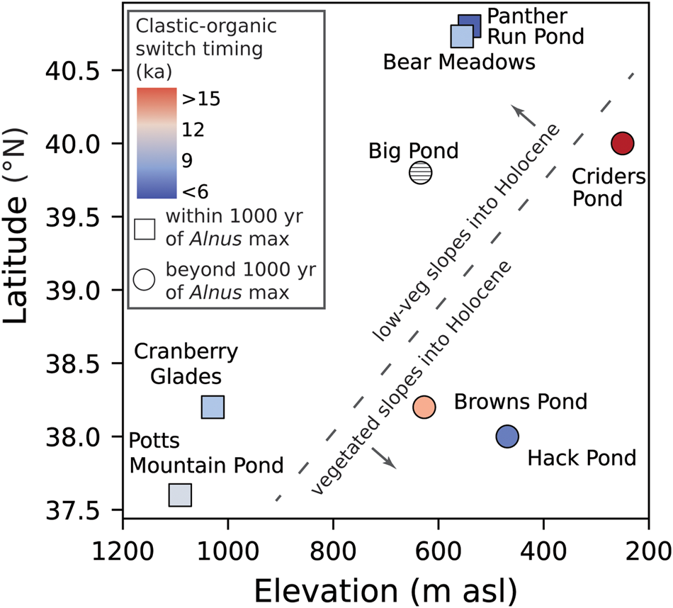
Figure 10. Relationship between latitude (°N), elevation, and pollen/stratigraphy patterns in unglaciated central Appalachian sites. Records taken from both higher elevations and latitudes tend to accumulate inorganic material for a longer time into the Pleistocene and Holocene (timing shown by color of symbol), implying that persistent cold conditions promoted clastic sedimentation. Step changes in pollen abundance of pioneer species of Alnus often correspond to a change in facies from inorganic to organic sedimentation (data shown as a square or circle if the switch occurred within or beyond 1000 yr of the record's Alnus peak abundance, respectively).
CONCLUSION
We synthesized basin-wide sedimentological observations with geochemical and pollen observations in cores to understand the provenance of sediment and surface processes in the context of local vegetation and global climate change. At Bear Meadows Bog, cold and dry conditions south of the Laurentide ice margin resulted in inorganic, dust-derived deposits until ca. 15 ka. Solifluction, which deposited coarse debris on basin margins, was active during the Bølling–Allerød interstadial, and sediment delivered to the basin at this time geochemically resembled locally sourced fines from the hillslopes. Based on this sedimentation history and pollen evidence for expansion of grasses in the basin during the BA, we interpret that initial warming following the LGM promoted deep hillslope disturbance via solifluction. In contrast, between ca. 10 and 9 ka, water level in the basin rose rapidly, concurrent with deposition of fines on basin margins and vegetation turnover, which we interpret as the consequence of increased rainfall and overland flow and absence of deep-seated erosion-driven processes like solifluction. Post-YD sediments geochemically resemble dust despite negligible dust flux in the Early Holocene, which we interpret as a flushing of dust stored on hillslopes by slopewash processes. We find that during late glacial warming, deep hillslope processes were driven predominantly by temperature changes rather than moisture. In contrast, during Early Holocene warming, overland flow caused widespread yet shallow hillslope erosion. Our interpretation that deep-seated hillslope disturbances occurred only during the first deglacial warming of the BA, and not in the Early Holocene following the YD, implies that permafrost may have been absent at our site during the YD. In upland periglaciated sites across Appalachia, clastic–organic sedimentation transitions are coincident with the presence of Alnus pollen such as at Bear Meadows, implying the onset of Early Holocene slopewash prior to the establishment of temperate forest is a regional trend.
Supplementary Material
The supplementary material for this article can be found at https://doi.org/10.1017/qua.2023.60.
Acknowledgments
Funding for this work came from a Penn State Institute for Energy and the Environment seed grant, a Geological Society of America and Quaternary Geomorphology and Geology Division graduate research student grant, and an American Association of Petroleum Geologists Grant-in-Aid. This research was conducted in Rothrock State Forest, funded and managed by the Pennsylvania Department of Conservation and Natural Resources, Bureau of Forestry. We thank Pat Drohan for field and sampling assistance, Brendan Culleton at the Penn State AMS Radiocarbon Lab for timely measurements, Danial Sukor and the Yale Analytical and Stable Isotope Center for conducting supporting laboratory analyses, Kalle Jahn for assistance coding the principal component analysis, and Adam Benfield for improving the manuscript text. We thank three anonymous reviewers and Eitan Shelef, as well as Associate Editor Terri Lacourse, for constructive feedback. Python and R files to generate data and figures can be found at https://doi.org/10.5281/zenodo.7573873.


 Open access