


INTRODUCTION
The densely populated central-northern Po Plain extends from the metropolitan agglomerate of Milan to the cities of Brescia, Cremona, and Verona, is seismically active, as proven by paleoseismological historical and instrumental records (e.g., Guidoboni and Comastri, Reference Guidoboni and Comastri2005; Livio et al., Reference Livio, Berlusconi, Michetti, Sileo, Zerboni, Trombino and Cremaschi2009; Albini and Rovida, Reference Albini and Rovida2010; Rovida et al., Reference Rovida, Locati, Camassi, Lolli and Gasperini2020, and references therein), geomorphological analyses of river diversion patterns (Burrato et al., Reference Burrato, Ciucci and Valensise2003), and large turbiditic events recorded in the Holocene stratigraphy of Lake Iseo (Lauterbach et al., Reference Lauterbach, Chapron, Brauer, Hüls, Gilli, Arnaud and Piccin2012; Rapuc et al., Reference Rapuc, Arnaud, Sabatier, Anselmetti, Piccin, Peruzza and Bastien2022). A clear geomorphological expression of tectonic activity in the area due to blind thrusting and fault-propagation folding is also provided by a series of isolated hillocks (Castenedolo, Ciliverghe, Monte Netto) with Early and middle Pleistocene sediments protruding from the surrounding late Quaternary plain (Desio, Reference Desio1965; Baroni and Cremaschi, Reference Baroni and Cremaschi1986; Baroni et al., Reference Baroni, Cremaschi, Fedoroff and Cremaschi1988; Livio et al., Reference Livio, Berlusconi, Michetti, Sileo, Zerboni, Trombino and Cremaschi2009, Reference Livio, Berlusconi, Zerboni, Trombino, Sileo, Michetti, Rodnight and Spötl2014, Reference Livio, Ferrario, Frigerio, Zerboni and Michetti2020; Zerboni et al., Reference Zerboni, Trombino, Frigerio, Livio, Berlusconi, Michetti, Rodnight and Spötl2015). Major seismic events in the area with magnitudes ranging from VII to IX on a Mercalli–Cancani–Sieberg (MCS) scale or 4–5 on a local magnitude (Ml) scale include the 1117 Verona, 1222 Brescia, 1661 Montecchio (Bergamo), 1799 Castenedolo (Brescia), 1802 Soncino (Cremona), 1901 Salò (Brescia), 2002 Iseo (Brescia), and 2004 Salò (Brescia) earthquakes (Guidoboni and Comastri, Reference Guidoboni and Comastri2005; Livio et al., Reference Livio, Berlusconi, Michetti, Sileo, Zerboni, Trombino and Cremaschi2009, and references therein).
Here we investigate long-term rates of vertical tectonic uplift in the belt of the Po Plain north of the above-mentioned isolated hills (southeast of the city of Brescia) by using a multidisciplinary stratigraphic approach. Guided by the previously determined general architecture of the Pleistocene glacial/fluvio-glacial/fluvial stratigraphy of the central-northern Po Plain subsurface, as constrained by magnetostratigraphically calibrated drill cores from the literature (Muttoni et al., Reference Muttoni, Carcano, Garzanti, Ghielmi, Piccin, Pini, Rogledi and Sciunnach2003; Scardia et al., Reference Scardia, Muttoni and Sciunnach2006, Reference Scardia, De Franco, Muttoni, Rogledi, Caielli, Carcano and Piccin2012), we describe the integrated stratigraphy of a new ~100-m-long drill core from Brescia (Brescia–Sant'Eufemia Core RL13, Fig. 3), in order to characterize the sedimentary environment on the basis of detailed facies analysis and better understand the major regional reflectors and the subsurface stratigraphy from well data.
We then compiled a database of 76 stratigraphic sections from well data in an area of 112 km2 centered around the neotectonic Castenedolo hillock (Fig. 1). We focus on two prominent and laterally continuous chronostratigraphic unconformities—the Red (R) and Yellow (Y) surfaces (Muttoni et al., Reference Muttoni, Carcano, Garzanti, Ghielmi, Piccin, Pini, Rogledi and Sciunnach2003)—whose regional geometries have been reconstructed from well data, outcrop data, seismic imaging, and interpolation methods. These data were used to calculate rates of sedimentation and vertical deformation (uplift or subsidence) of the investigated area during the Pleistocene.
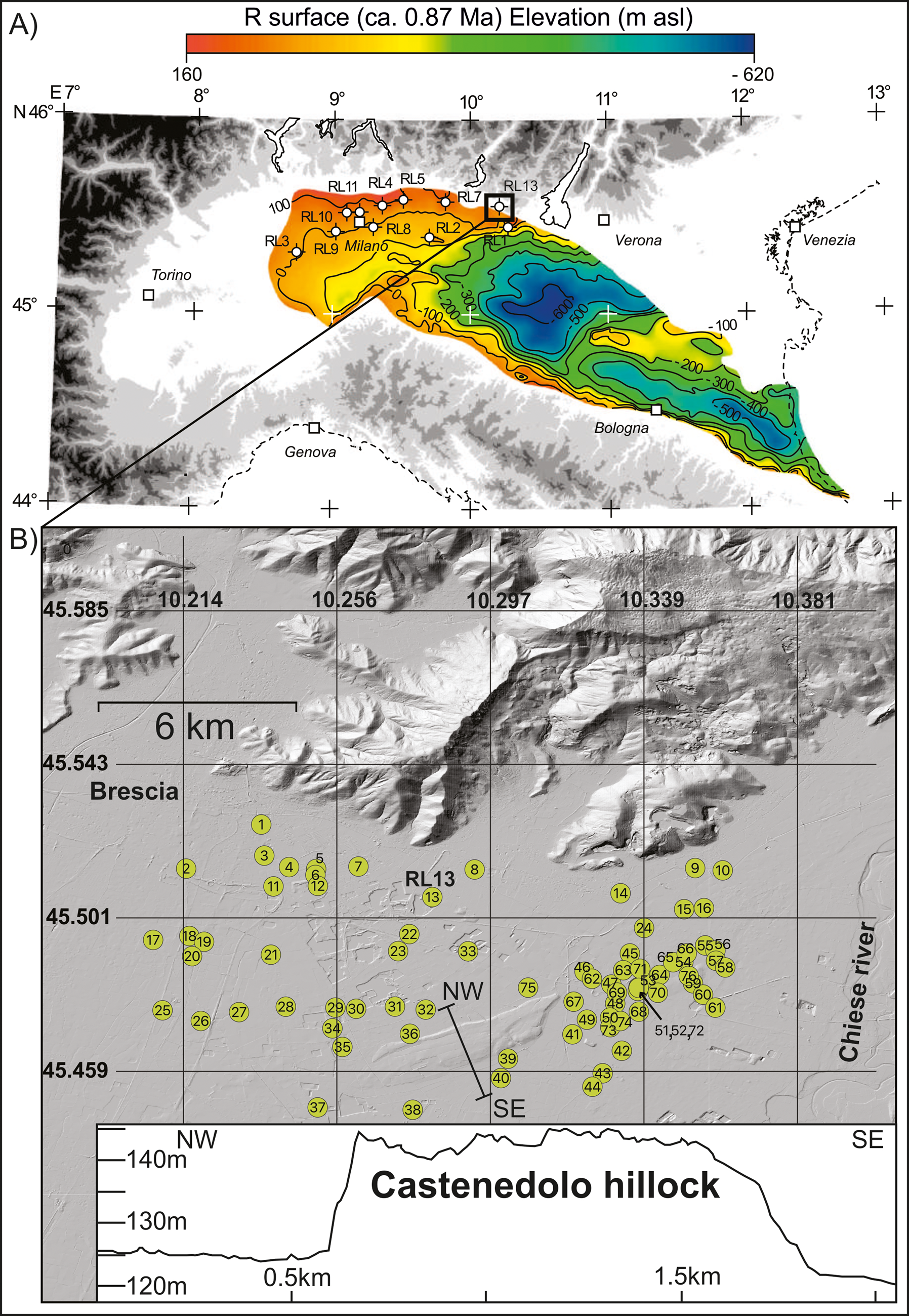
Figure 1. (A) Location of the RL drill cores (RL1-Ghedi, RL2-Pianengo, RL3-Cilavegna, RL4-Agrate, RL5-Trezzo, RL7-Palosco, RL8, RL9, RL10, RL11, and RL13-Brescia Sant'Eufemia), in the context of the Po Plain and the bordering Alps and Apennines. Isobaths in m of the R subsurface from 100 m in red to −600 m in blue (data from Scardia et al., Reference Scardia, De Franco, Muttoni, Rogledi, Caielli, Carcano and Piccin2012). (B) Close up of the study area, shaded digital elevation model of the Brescia basin area showing the southern Alps and the Castenedolo hillock. Location of RL13 drill core and of 76 stratigraphies from well data. Line trace and Castenedolo morphology are also represented.
PLEISTOCENE CHRONOSTRATIGRAPHY OF THE CENTRAL-NORTHERN PO PLAIN
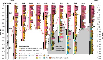
According to published seismic data, facies analysis, and magneto-biostratigraphy, the Pleistocene stratigraphy of the central-northern Po Plain is arranged in three main depositional sequences, termed from older to younger PS1, PS2, and PS3 (Fig. 2), that are bounded by the two aforementioned main unconformities represented by the R and Y surfaces (Ori, Reference Ori1993; Di Dio, Reference Di Dio1998; Carcano and Piccin, Reference Carcano and Piccin2002; Muttoni et al., Reference Muttoni, Carcano, Garzanti, Ghielmi, Piccin, Pini, Rogledi and Sciunnach2003; Scardia et al., Reference Scardia, Muttoni and Sciunnach2006, Reference Scardia, De Franco, Muttoni, Rogledi, Caielli, Carcano and Piccin2012). Sequence PS1 is late Early Pleistocene age, from ca. 1.4 Ma to ca. 0.87 Ma, straddling the Jaramillo subchron (1.070–0.99 Ma; time scale of Channell et al., Reference Channell, Singer and Jicha2020, used through), and consists of silt and clay packages alternating with fine- to medium-grained sand interpreted as having been deposited in low-subsidence meandering river-plain settings with sediment sourced mainly in the Western and Central Alps (Muttoni et al., Reference Muttoni, Carcano, Garzanti, Ghielmi, Piccin, Pini, Rogledi and Sciunnach2003; Garzanti et al., Reference Garzanti, Vezzoli and Andò2011; Scardia et al., Reference Scardia, De Franco, Muttoni, Rogledi, Caielli, Carcano and Piccin2012). This meandering river system passed eastward towards the Adriatic Sea to shallow marine and transitional deposits (Kent et al., Reference Kent, Rio, Massari, Kukla and Lanci2002; Scardia et al., Reference Scardia, Muttoni and Sciunnach2006).

Figure 2. Revised summary graphic log of the RL drill cores from the central Po Plain showing regional depositional sequences (PS1, PS2, and PS3), main lithologies, sedimentary environments, and paleosols. Y (0.45 Ma) and R (0.87 Ma) seismic subsurfaces and magnetostratigraphy as reported by previous authors.
At ca. 0.87 Ma in the late Early Pleistocene (post-Jaramillo Matuyama), the R surface/sequence boundary formed in consequence of the broadly synchronous and rapid progradation of PS2 braid-plain deposits over the PS1 meandering river plain at the onset of the major Pleistocene glaciations in the Alps (Muttoni et al., Reference Muttoni, Carcano, Garzanti, Ghielmi, Piccin, Pini, Rogledi and Sciunnach2003). Sequence PS2 consists of thick packages of alternating medium- to coarse-grained sand, gravel, and subordinate silt, interpreted as deposited in glacial outwash braid-plain settings, which prograded from the proximal Southern Alps southward towards, and above, the PS1 meandering river plain (Muttoni et al., Reference Muttoni, Carcano, Garzanti, Ghielmi, Piccin, Pini, Rogledi and Sciunnach2003; Garzanti et al., Reference Garzanti, Vezzoli and Andò2011; Scardia et al., Reference Scardia, De Franco, Muttoni, Rogledi, Caielli, Carcano and Piccin2012).
PS2 is bounded at the top by the Y surface, placed using magnetostratigraphy from several drill cores (including core RL13 from this study) systematically in the Brunhes chron at around 0.45 Ma (Scardia et al., Reference Scardia, De Franco, Muttoni, Rogledi, Caielli, Carcano and Piccin2012), albeit its precise age remains uncertain. Sequence PS3 above the Y surface was deposited during the middle–late Pleistocene and consists almost exclusively of coarse-grained, poorly sorted, and crudely bedded gravel of proximal outwash braid-plain settings that prograded over the PS2 distal braid-plain deposits (Scardia et al., Reference Scardia, De Franco, Muttoni, Rogledi, Caielli, Carcano and Piccin2012; Badino et al., Reference Badino, Pini, Ravazzi, Margaritora, Arrighi, Bortolini and Figus2020). The scarce lateral traceability of seismic reflectors suggests that deposition occurred in a confined network of laterally shifting fluvial channels with low accommodation space (Scardia et al., Reference Scardia, De Franco, Muttoni, Rogledi, Caielli, Carcano and Piccin2012).
THE SEDIMENTARY SUCCESSION FROM CORE RL 13: METHODS AND RESULTS
Lithostratigraphy and sedimentology
In a joint effort to study the recent seismic activity of the central Po Plain (Norini et al., Reference Norini, Aghib, Di Capua, Facciorusso, Castaldini, Marchetti and Cavalin2021), a 100-m-long drill core with an average recovery of 95% (hereafter referred to as RL 13) was drilled at Brescia Sant'Eufemia (Fig. 1) and studied for lithostratigraphy, soil stratigraphy, sandstone petrography, facies analysis, and magnetostratigraphy, in order to better constrain the stratigraphic evolution of the area. The recovered sedimentary record consists of a variety of terrigenous clastic fluvial lithologies ranging from coarse- to fine-grained sands to fine-grained sediments related to the main regional depositional sequences PS1, PS2, and PS3 described above. In particular, the sedimentary record consists, from top to bottom, of the following sequences (depths are in meters below the rig floor [mbrf]) (Fig. 3, Supplementary data, Table I).
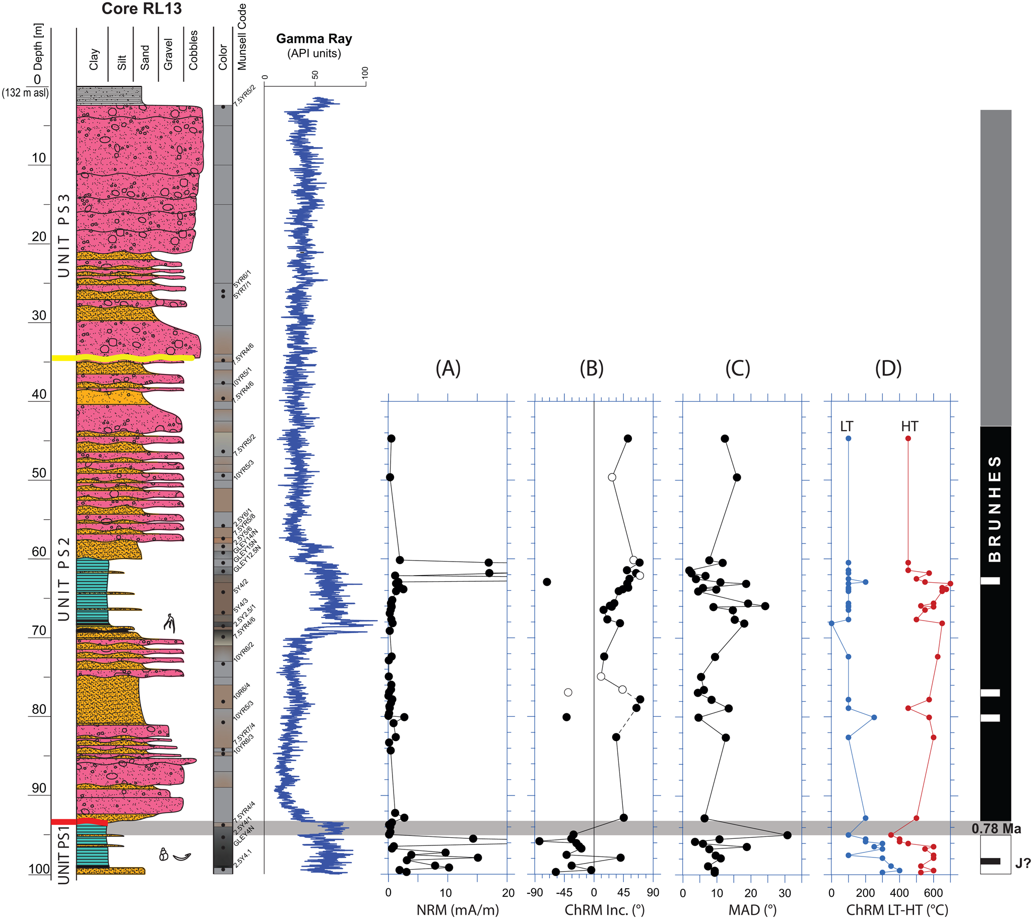
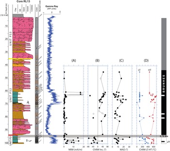
Figure 3. Stratigraphic outline of RL 13 drill core. From left to right: Depths in mbrf (m below rig floor); regional depositional units (PS1, PS2, and PS3); lithology with colors codified according to the Munsell Color Chart (Munsell Color, 2020). The Y surface is highlighted in yellow; the R surface is most probably eroded in core RL13 and is contained in the unconformity between Units PS1 and PS2. To the right of the lithology column is the (SGR) spectral gamma ray in API units. For magnetostratigraphic data: (A) is the intensity of the natural remanent magnetization (NRM), (B) is the characteristic remanent magnetization inclination values (ChRM Inc.) component directions used for magnetic polarity interpretation, (C) is the maximum angular deviation (MAD) values of the ChRM component directions, and (D) is a plot of the unblocking temperature windows of the ChRM component directions (from low temperature, LT, to high temperature, HT). To the right is a plot of the interpreted magnetic polarity, with black bars representing normal polarity and white bars reverse polarity; J? = Jaramillo? See text for discussion.
PS3: 2.40–34.60 mbrf
PS3 consists of massive, poorly sorted coarse to very coarse sandy gravels, containing clasts 5–10 cm in size. Clasts are predominantly composed of sedimentary lithologies (limestones and volcanic sandstones), and to a lesser extent of volcanic lithologies. Coarse lithologies and sedimentary features are consistent with deposition in a high energy, proximal alluvial fan setting. The Y erosional surface that marks the base of PS3 is placed at 34.60 mbrf, which corresponds to a sharp color change from gray sediments (Munsell Color, 2000; code 7.5 YR 5/2) to yellowish-gray sediments (5YR 6/1). The Y surface rests on a 40-cm-thick paleosol.
PS2: 34.60–93.37 mbrf
PS2 consists of two or perhaps three fining-upward cycles of mainly sands and sandy gravels representing recurrent lateral migrations of the river system. The first cycle from the top, located 34.60–57.30 mbrf, is not complete, and is truncated by the Y erosional surface at its top. The base of PS2 is placed at 93.70 mbrf and corresponds to an erosional surface that is interpreted to approximate the R surface in highly energetic, proximal settings such as RL13. Paleosols have been recognized within the record at 34.60, 57.30, 57.70, and 68.90 mbrf.
PS1: 93.37–100 mbrf
PS1, mostly composed of fine-grained lithologies resting below the R erosional surface, is interpreted as deposited in a meandering river-plain setting on the basis of its sedimentary features, including common lamination, water structures, presence of organic matter, and frequent fossil remains (mainly gastropods).
Micropedological characterization of paleosols
Eighteen levels corresponding to visible color and texture variations were sampled within unit PS2 for micromorphological analyses. The undisturbed samples were impregnated under vacuum in polyester to obtain thin sections (Murphy, Reference Murphy1986). Slides were observed using a petrographic microscope under plain and cross-polarized light and oblique incident light. Interpretations (Supplementary data, Table II) rely on the principles described in Stoops et al. (Reference Stoops, Marcelino and Mees2018) and in Stoops (Reference Stoops2021).
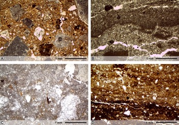
Samples from levels at 34.60, 57.30, 57.70, and 68.90 mbrf show evidence of pedoplasmation and the development of soil aggregates and soil fabric (Fig. 4A) in association with other pedogenetic features, including Fe/Mn nodules and impregnations related to redoximorphic processes, as well as clay coatings produced by illuviation. These levels formed after exposure to the atmosphere and can therefore be interpreted as truncated paleosols based on the micropedological indicators suggested by Cremaschi et al. (Reference Cremaschi, Trombino, Zerboni, Stoops, Marcelino and Mees2018). These paleosols likely developed under stable temperate environment conditions.
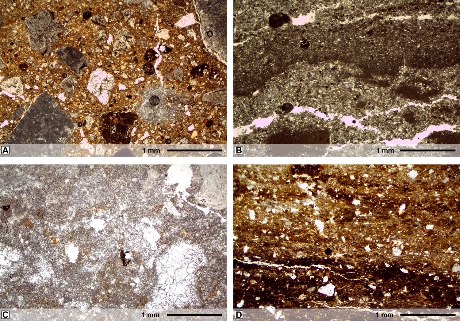
Figure 4. Photomicrographs representing the different types of anomalies recognized in thin sections. (A) Well-developed paleosol showing aggregation of the matrix and iron oxide formation (BS1P1); (B) sedimentary laminations partially impregnated by iron (BS1P6); (C) strongly cemented calcrete (BS1P2; (D) accumulation of reddened organic material (BS1P13).
Six other samples at 36.30, 38.70, 43.90, 44.70, 50.85, and 53,80 mbrf, with a mesoscale appearance similar to the paleosols described above, instead show only features related to transport of weathered material (former soil debris). Furthermore, reddening caused by the accumulation of iron oxyhydroxides transported in solution is also widespread and is related to groundwater oscillation promoting hydromorphic conditions (Fig. 4B). Two of the samples contain evident clayey rounded fragments compatible with sedimentary redeposition of soil material (pedorelicts). These levels do not therefore represent in situ-formed soils, but are the result of soil reworking and redeposition, and are interpreted as geological pedorelicts (sensu Cremaschi and Rodolfi, Reference Cremaschi and Rodolfi1991).
Five other samples at 35.50, 37.70, 77.30, 82.60, and 88.70 mbrf show abundant carbonate cementation, with calcite crystals dispersed in the groundmass forming complex calcitic pedofeatures (Fig. 4C); such evidence is likely related to the formation of calcretes. It is unclear whether these calcretes formed as consequence of surface pedogenesis (thus representing buried Bk soil horizons) or soil–groundwater interactions. Two additional samples at 68.68 and 69.20 mbrf are characterized by a groundmass strongly impregnated by Fe/Mn oxi-hydroxides and intercalated with layers of dark/black fibrous organic material (Fig. 4D). These features suggest redoximorphic processes related to deposition of iron oxides/hydroxides at the bottom of a wetland environment (“bog iron”; Kaczorek and Sommer, Reference Kaczorek and Sommer2003). Finally, a sample collected at 99.20 mbrf from unit PS1 has been interpreted as an organic-rich “sapropel-type” level for its finely laminated pattern consisting of an alternation of organic material and silt.
Sand petrography
For petrographic analyses, we studied 26 samples that were impregnated with araldite, cut into standard thin sections, and stained with alizarine red for limestone versus dolostone distinction. On each thin section, at least 300 points were counted following the QFL Gazzi-Dickinson method (Ingersoll et al., Reference Ingersoll, Bullard, Ford, Grimm, Pickle and Sares1984), and sands were classified according to their main components (Dickinson, Reference Dickinson1970). Point-counts revealed that the 26 sandstone layers can be grouped into two main petrofacies: A (21 samples) and B (5 samples) (Supplementary data, Table III). In petrofacies A (Fig. 5A, B), recognized in coarse-grained layers recovered at 0–60 mbrf and 70–93 mbrf, the lithic fraction dominates over the single-minerals fraction (>70% of the QFL particles), and includes limestones, dolostones, and terrigenous fragments, with subordinate volcanic and metamorphic fragments (<20% of the lithic fraction). The single-minerals fraction includes monocrystalline quartz, polycrystalline quartz, rare K-feldspar, and heavy minerals (HM: biotite, chlorite, garnet, and amphibole). Monocrystalline quartz often shows a straight extinction, typical of volcano-derived crystals. In petrofacies B (Fig. 5A, C), identified in the fine-grained layers recovered at 60–70 mbrf, as well as 93–100 mbrf, the single-minerals fraction exceeds the lithic fraction and is dominated by monocrystalline quartz with straight extinction as well as polycrystalline quartz, with subordinate feldspar, biotite, muscovite, and chlorite. The lithic fraction includes volcanic (rhyolites and andesites), metamorphic (gneiss and schists), and very rare sedimentary (limestones) lithics.
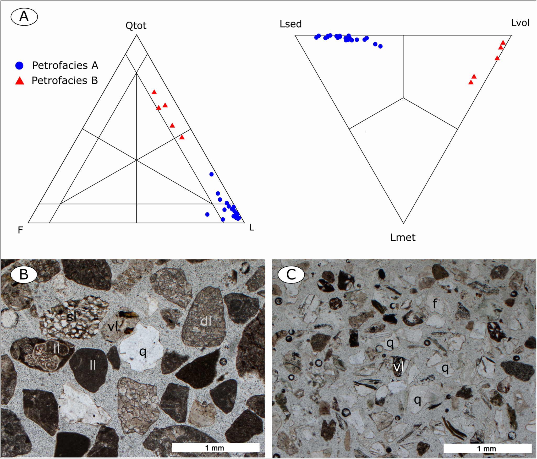
Figure 5. Sand petrography of RL13 drill core. (A) Detrital modes of the RL13 sands. Qtot = mono- and polycrystalline quartz; F = feldspars; L = lithic grains (Lsed = sedimentary lithics; Lvol = volcanic lithics; Lmet = metamorphic lithics). (B) Typical detrital assemblage of Petrofacies A; sedimentary lithics are the most abundant component. (C) Typical detrital assemblage of Petrofacies B; quartz is the most abundant component. Both microphotographs are under parallel nichols: q = quartz; f = feldspar; dl = dolostone lithic; ll = limestone lithic; sl = terrigenous lithic; vl = volcanic lithic.
Petrofacies A, largely dominated by calcareous lithics with subordinate porphyritic volcanic and gneissic metamorphic lithics, as well as single minerals of quartz and micas, was produced mainly by erosion of the Permo-Mesozoic volcano-sedimentary cover cropping out to the North of the depositional area, and transported by a local, N-S trending fluvial network (see also Muttoni et al., Reference Muttoni, Carcano, Garzanti, Ghielmi, Piccin, Pini, Rogledi and Sciunnach2003, for similar data and interpretation from nearby drill cores). Instead, detritus of petrofacies B, which is characterized by large amounts of quartz, subordinate feldspar, and minor amounts of lithics, reflects higher sediment supply from the internal sector of the alpine belt dominated by metamorphic terrains. Similar petrofacies documented in the Pianengo drill core (Muttoni et al., Reference Muttoni, Carcano, Garzanti, Ghielmi, Piccin, Pini, Rogledi and Sciunnach2003) and in the Ghedi drill core (Garzanti et al., Reference Garzanti, Vezzoli and Andò2011; RL2 and RL1, respectively, in Fig. 2) were interpreted as related to changes in paleodrainage during glacial–interglacial cycles (Muttoni et al., Reference Muttoni, Carcano, Garzanti, Ghielmi, Piccin, Pini, Rogledi and Sciunnach2003, Garzanti et al., Reference Garzanti, Vezzoli and Andò2011). Alternatively, or in addition to this interpretation, changes in petrofacies could have been triggered by climatically controlled changes in erosion rates and related sediment supply during glacial–interglacial cycles (e.g., Monegato and Vezzoli, Reference Monegato and Vezzoli2011).
Magnetostratigraphy
Paleomagnetic properties of core RL13 were studied on a total of 70 cubic (~8 cm3) samples collected from cohesive, fine-grained sediments 44.72–99.72 mbrf of the core stratigraphy (Fig. 3). Nine of these samples were subjected to rock magnetic analyses by means of backfield acquisition of an isothermal remanent magnetization (IRM) from −2.5T to +2.5T and thermal demagnetization of a three-component IRM imparted in fields of 2.5T, 0.4T, and 0.12T. The remaining 61 samples were subjected to demagnetization of the natural remanent magnetization (NRM) for magnetic polarity interpretation: 50 samples were subjected to thermal demagnetization in steps of 50°C or 25°C up to a maximum of 650°C, and 11 samples to alternating field (AF) demagnetization up to 100mT. The NRM was measured after each demagnetization step with a 2 G Enterprises DC-SQUID cryogenic magnetometer located in a shielded room.
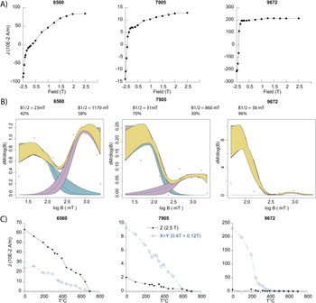
The intensity of the NRM was found to vary in the range 0.1–5 mA/m for most of the sampled levels, except for clay levels at around 60–65 mbrf and 94–100 mbrf where the NRM varies in the range 10–100 mA/m (Fig. 3A). IRM backfield acquisition curves of representative samples (Fig. 6A) show an initial steep growth at low fields that is either followed by a gentle slope with no saturation up to 2.5T (samples 6560, 7905) or by saturation at ~200–250mT (sample 9672). Unmixing magnetic coercivity distributions following Maxbauer et al. (Reference Maxbauer, Feinberg and Fox2016) reveals that the low coercivity component has B1/2 (field at which half of saturation IRM is acquired) of ~20–40 mT, while the high coercivity component, when present, has B1/2 on the order of 1T (Fig. 6B). Thermal demagnetization of a three-component IRM reveals maximum unblocking temperatures of ~570°C for the medium-low (0.4–0.12T) coercivity components, and ~680°C for the high (2.5T) coercivity component (Fig. 6C). These results are collectively interpreted as indicating the presence of variable mixtures of (titano)magnetite and hematite.
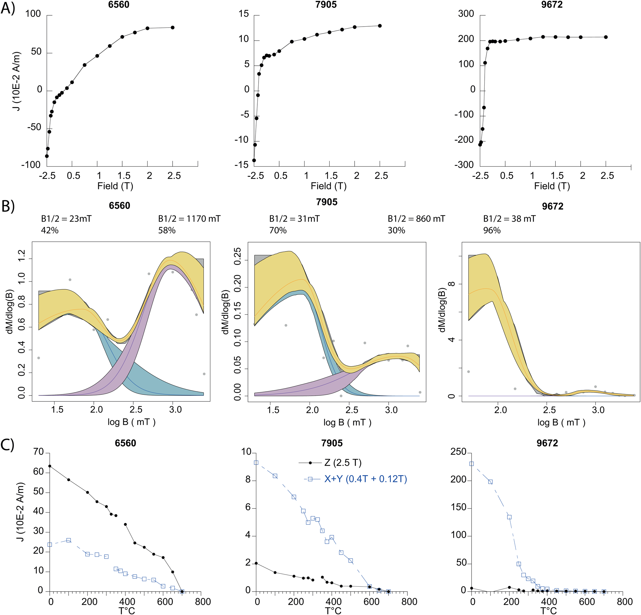
Figure 6. (A) IRM backfield acquisition curves of representative samples from core RL13. (B) Coercivity unmixing of the same curves (Maxbauer et al., Reference Maxbauer, Feinberg and Fox2016) allowed identification of two coercivity components differing for B1/2 and relative proportion (%). For each panel, the blue curve (with uncertainty envelope) represents the low-coercivity phase, the purple curve represents the high-coercivity phase, and the yellow curve represents the over (unmixed) coercivity distribution. (C) Thermal decay of a three-component IRM on the same samples. These experiments collectively show the occurrences of various proportions of (titano)magnetite and hematite (samples 6560 and 7905) or virtually only (titano)magnetite (sample 9672).
Orthogonal projections of thermally demagnetized data (Supplementary Table IV) indicate the existence of a characteristic remanent magnetization (ChRM) component with either positive (down-pointing) inclinations (Fig. 7A, samples 6144 and 6253) or negative (up-pointing) inclinations (Fig. 7A, samples 8005 and 9752) that were removed to the origin of the demagnetization axes on 39 samples between ~100°C and ~400–680°C. AF demagnetized data (Supplementary Table V) reveal the existence in six samples of a similar ChRM component isolated between 5 mT and 70–100 mT.
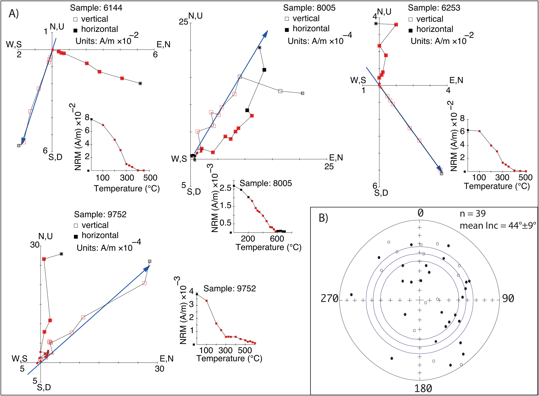
Figure 7. (A) Orthogonal projections of thermal demagnetization data of selected samples from Core RL13. Open (closed) symbols are projections on to the vertical (horizontal) plane. Cores were not oriented with respect to geographic north, hence only magnetic inclination was used to interpret magnetic polarity stratigraphy. Diagrams made with PuffinPlot (Lurcock and Wilson, Reference Lurcock and Wilson2012). (B) Equal-area projection of the ChRM component directions. Inclination-only statistics indicate a mean value of 44 ± 9° while declination values are randomly distributed because core RL13 was not oriented relative to north.
Standard least-square analysis was used to calculate orientation and maximum angular deviation (MAD) values of these ChRM component directions (Supplementary Table VI). Because core RL13 was not oriented with respect to the geographic north, we could use only the inclination of the ChRM component vectors to outline magnetic polarity stratigraphy, resulting the associated declination values being randomly distributed (Fig. 7B). The ChRM inclination values of samples from units PS3 and PS2 indicate dominant normal magnetic polarity, referred to the Brunhes chron (C1n; <0.773 Ma) (Fig. 3B). The underlying sediments of unit PS1 down to core bottom bear reverse magnetic polarity attributed to the late Matuyama chron (C1r.1r; 0.773–0.99 Ma) (Fig. 3B), acknowledging also previous data and interpretations from similar and nearby cores (Fig. 2; Muttoni et al., Reference Muttoni, Carcano, Garzanti, Ghielmi, Piccin, Pini, Rogledi and Sciunnach2003; Scardia et al., Reference Scardia, Muttoni and Sciunnach2006, Reference Scardia, De Franco, Muttoni, Rogledi, Caielli, Carcano and Piccin2012). The MAD values of these ChRM directions are on the order of 10 ± 5° (Fig. 3C), while the unblocking windows reside in the (titano)magnetite–hematite temperature range with no correlation with lithology or stratigraphic position (Fig. 3D). The Brunhes–Matuyama boundary (0.773 Ma) is therefore placed at 93.70 mbrf at the PS1/PS2 erosional boundary (Fig. 3). In more complete sedimentary settings, the R surface and onset of PS2 deposition occur at ca. 0.87 Ma before the Brunhes–Matuyama boundary (e.g., core Pianengo RL2, Muttoni et al., Reference Muttoni, Carcano, Garzanti, Ghielmi, Piccin, Pini, Rogledi and Sciunnach2003; see also Scardia et al., Reference Scardia, Muttoni and Sciunnach2006, Reference Scardia, De Franco, Muttoni, Rogledi, Caielli, Carcano and Piccin2012). We therefore infer that the R surface in core RL13 has been eroded by the basal PS2 high-energy gravels. As for the Y surface, according to sedimentological and facies analysis, it was placed at ~35 mbrf, which is well within the Brunhes chron.
MODELING OF THE R AND Y REGIONAL UNCONFORMITIES IN THE BRESCIA AREA
With the purpose of modeling the R and Y surfaces, which represent the regional unconformities for the Brescia area, we used three different datasets.
One dataset, which consisted of seventy-six drillings, including core RL13 of this study and additional drill cores from the literature (Fig. 2), and natural gamma-ray logs, was analyzed to identify the R and Y unconformities in a 112-km2 area around Castenedolo using sedimentary and color patterns (i.e., coarser sediments overlying finer sediments) similar to the patterns observed in the reference drillings shown in Figures 2 and 3. In the natural gamma ray logs, the R surface has been identified as a sharp change of the spectral gamma ray API unit (American Petroleum Institute, 1974) (Fig. 3). A subset of 48 lithostratigraphic logs and 15 natural gamma ray logs showing the R and/or Y surfaces was included in a 3D GIS database (Fig. 8A). Well-head elevations were extracted from a 5-m-resolution digital elevation model (DEM). The elevations above sea level of the R and Y surfaces were calculated by subtracting depths measured in well logs from well-head elevations.
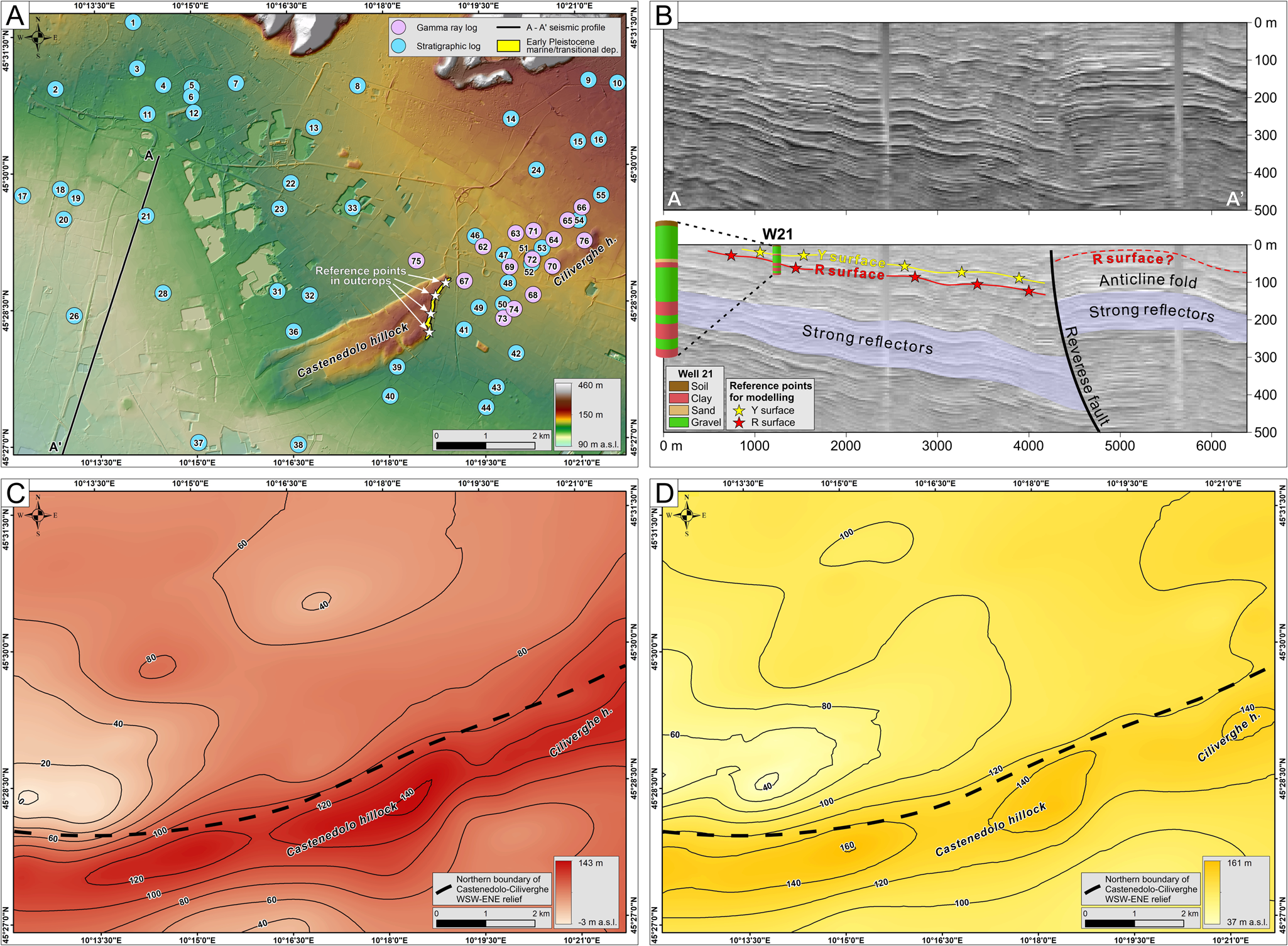
Figure 8. (A) Map of the study area over a shaded digital elevation model (DEM) with elevation color scale. Locations of the lithostratigraphic logs, natural gamma ray logs, outcrops of Early Pleistocene marine/transitional deposits, and trace (A–A′) of the seismic reflection profile used for modeling the R and Y regional unconformities are shown. (B) Pseudo-relief image of the time-depth converted seismic reflection profile and its interpretation with the R and Y surface reflectors, fault-propagation fold, and well W21. (C) Map of the modeled R surface. (D) Map of the modeled Y surface.
In addition to the drillings, a second dataset of Early Pleistocene marine/transitional deposits cropping out along the southeastern slope of the Castenedolo hillock were considered. These outcrops indicate that the R and the shallower Y unconformities intersect the present topographic surface and/or were partly eroded in the southern sector of the study area (Fig. 8A). The topographic elevation of the top of the transitional/marine sediments, calculated from the DEM, was used to constrain the geometry of the R surface in this key area.
Finally, a dataset consisting of a pseudo-relief image elaborated from a 6.3-km-long segment of an available seismic reflection profile from within the study area was included in the 3D GIS database (Fig. 8A, B) (Livio et al., Reference Livio, Berlusconi, Michetti, Sileo, Zerboni, Trombino and Cremaschi2009). This depth-converted (velocity for conversion 1800 m/s), pseudo-relief seismic image extends down to 500 m below the ground surface. The R and Y unconformities also have been identified in a well close to the seismic line (well 21, D6C267358372 in Supplemental Table I, Fig. 8A, B). The R surface in this well corresponds to a clear southward-dipping reflector in the seismic profile (Fig. 8B). The reflector is displaced by a southward-dipping reverse fault, where the seismic profile shows an asymmetric anticline fold to the south truncated against the fault plane. This fault-propagation fold defines an uplift of the R unconformity south of the reverse fault plane, also displacing and folding deeper strong reflectors identified on both sides of the fault plane (Fig. 8B). The Y surface also corresponds to a reflector in the seismic profile that has a geometry similar to that of the R surface (Fig. 8B). Both reflectors have been used in the 3D GIS model to constrain the geometry of the R and Y unconformities in the western sector of the study area (Fig. 8B).
The geometries of the R and Y surfaces, reconstructed throughout the investigated drillings, the available outcrops, and the seismic profile, show higher elevations in the southern part and a depocenter in its central-northern sector (Fig. 8A, B). Elevation data have been used as reference points for the geometric modeling of the R and Y unconformities. We interpolated these reference points by regularized spline with tension continuous polynomial function. This interpolation method was used because of its capability to approximate geological surfaces, minimizing overall curvature and small-scale variations, resulting in smooth grids that pass through the sampling points (e.g., Mitášová and Hofierka, Reference Mitášová and Hofierka1993; Mitášová and Mitas, Reference Mitášová and Mitáš1993; Norini et al., Reference Norini, Capra, Groppelli, Agliardi, Pola and Cortes2010a, Reference Norini, Capra, Borselli, Zuniga, Solari and Sarocchib).
Geometric modeling of the R surface shows the presence of a WSW-ENE elongated relief with a maximum elevation of about 140 m asl. This elongated structure coincides with the morphological major axis of the Castenedolo and Ciliverghe hillocks (Fig. 8C). The central northern sector of the area shows medium to low elevations of the R surface (0–60 m asl). Similarly, the Y surface defines a sharp WSW-ENE-trending ridge in the southern sector of the area with a maximum elevation of about 160 m asl and lower elevations in the central and northern sector (40–100 m asl) (Fig. 8D).
Seismic imaging indicates that the elongated relief defined by the R and Y surfaces coinciding with the Castenedolo–Ciliverghe morphostructure corresponds to a fault-related anticline fold bounded northward by a reverse fault, suggesting Quaternary compressional tectonics (Fig. 8B). Reduced thickness of the sedimentary succession to the south of the fault plane suggests progressive displacement during sedimentation (Fig. 8B). The northern boundary of the WSW-ENE-trending Castenedolo and Ciliverghe relief (e.g., Fig. 8C, D), and the attitude and curvature of the growth fault identified in the seismic section (Fig. 8B), provided the geometric constraints that have been used to model the 3D fault geometry. The three-dimensional shape of the fault was calculated with a GIS algorithm projecting the fault plane imaged in the seismic profile along the fault trace defined by the northern boundary of the WSW-ENE-trending relief (Fig. 9A, B) (e.g., Norini et al., Reference Norini, Baez, Becchio, Viramonte, Giordano, Arnosio, Pinton and Groppelli2013). This geometric modeling represents a continuous curved fault plane cutting through the R and Y unconformities below the present topographic surface (Fig. 9C, D).
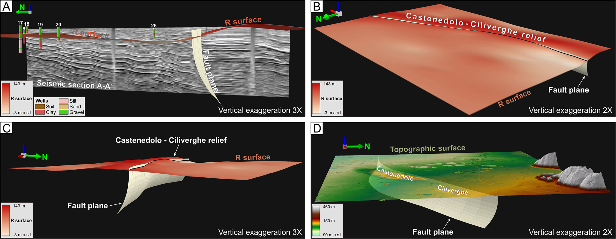
Figure 9. (A) Reconstruction of the fault plane geometry with depth, based on the mapped fault trace (Fig. 8C, D), modeled R surface, and seismic reflection profile. (B) Perspective view from NW of the fault plane and modeled R surface. (C) Perspective view from ENE of the fault plane and modeled R surface. (D) Perspective view from E of the fault plane and shaded DEM with elevation color scale.
DISCUSSION: PLEISTOCENE TECTONO-STRATIGRAPHIC EVOLUTION OF THE CASTENEDOLO AND CILIVERGHE AREA
Three depositional sequences were emplaced in the last ca. 0.87 Ma in the study area: (1) PS1 (> ca. 0.87 Ma) formed along a meandering river setting; (2) PS2 (0.87–0.45 Ma) corresponding to distal braided river setting showing 2–3 cycles of lateral channel migration and/or avulsion, and (3) PS3 (<0.45 Ma) belonging to a proximal braided river environment (Fig. 3). These sequences are interlayered with paleosols and other soil-like levels. Micropedology allowed us to discriminate between real in situ-formed paleosols, reworked soil material, and other deposits in core RL13, leading to more accurate interpretations of phases of subaerial conditions. Most of the paleosols were identified within the PS2 sequence and at the base of the PS3 unit, marking the passage from a distal (PS2) to a proximal (PS3) braided fluvial system.
The three depositional sequences are bounded by the R and Y unconformities. Considering the RL13 sedimentary record, the top of unit PS1 corresponds to the R unconformity (ca. 0.87 Ma) eroded by the basal PS2 high-energy gravels, and the top of the PS2 sequence represents the regional Y unconformity (ca. 0.45 Ma) where a well-developed paleosol has been identified (Fig. 3). The sedimentary record of the study area indicates that these unconformities were generated by sedimentary processes related to changes in energy, sediment transport, paleodrainage flow, and erosion regime over a wide alluvial plain. This suggests that they formed almost synchronously as horizontal and planar surfaces at the scale of the study area (112 km2). The measurement of deviations from planarity and the age constraints of the R and Y surfaces allow estimation of the long-term rates of tectonic deformation and the sedimentation/weathering/erosion net balance over the study area, as follows.
First, the mean elevation of the R unconformity in the northern sector of the study area is ~50 m asl, while the same surface reaches 120–140 m asl to the south, on top of the elongated ridge shown by geometric modeling, which indicates a mean uplift of ~80 m (Figs. 8C, 9A). The resulting mean vertical displacement rate is in the range of 0.09 mm/yr during the last ca. 0.87 Ma, which is consistent with similar results from the adjacent western area (e.g., Perini et al., Reference Perini, Muttoni, Livio, Zucali, Michetti and Zerboni2023). The Y surface has an elevation of ~100 m asl in the northern sector of the area and an elevation of 140–160 m asl on top of the elongated ridge (Fig. 8D), yielding an uplift of ~50 m and a mean vertical displacement rate of about 0.11 mm/yr in the last ca. 0.45 Ma. These calculations suggest a nearly constant relative uplift of ~0.1 mm/yr in the last ca. 0.87 Ma.
Second, a recent fault crossing the study area and driving the observed tectonic uplift has been identified and its geometry defined for the first time (fault trace in Fig. 8C, D, and 3D shape in Fig. 9). The modeling of this southward dipping fault generating tectonic uplift and anticline folding shows a mean dip angle of the fault plane of 45°. This means that the horizontal displacement rate is ~0.1 mm/yr, giving a northward tectonic shortening over the last ca. 0.87 Ma in the range of 80–90 m within the study area.
Third, the volume of alluvial sediments between the modeled R and Y surfaces is ~4.2 km3 in the 112-km2 area, resulting in a mean sedimentation/erosion net balance of about +8.9 cm/kyr from ca. 0.87 Ma to ca. 0.45 Ma (~0.09 mm/yr). The volume of alluvial sediments between the Y unconformity and the present topographic surface is ~2.9 km3 in the study area, giving a mean sedimentation/erosion net balance rate of about +5.8 cm/kyr in the last ca. 0.45 Ma (~0.06 mm/yr). These calculations indicate a decrease with time of the sediment accumulation rate over the last ca. 0.87 Ma.
These calculations suggest that the recent fault shown in Figure 9 deformed the sedimentary succession with similar average vertical and horizontal displacement rates estimated over two different time intervals (0.87–0.45 Ma, and 0.45 Ma–present). In contrast, alluvial sedimentation/weathering/erosion net balance showed a positive budget that decreased during time. From ca. 0.87 Ma to ca. 0.45 Ma (PS2 depositional sequence), tectonic uplift and mean alluvial sediment accumulation were almost the same (~0.09 mm/yr). After ca. 0.45 Ma (PS3 depositional sequence), tectonic uplift remained nearly constant (~0.1 mm/yr), while alluvial sediment accumulation significantly decreased (~0.06 mm/yr). This indicates that tectonic deformation gradually increased its importance in the middle Pleistocene as a geomorphic factor over alluvial sedimentation and erosion. Since ca. 0.45 Ma, the tectonic uplift rate of the Castenedolo and Ciliverghe tectonic structure was significantly greater than the sediment accumulation rate, allowing the WSW-ENE-trending relief to emerge gradually from the alluvial plain at a mean rate of ca. 0.04 mm/yr (difference between the estimated uplift and sediment accumulation rates constrained by the age of the Y surface). At this rate, the hillocks reached an elevation of ~18 m in ca. 0.45 Ma. This height corresponds to the present-day elevation of the Castenedolo hillock above the alluvial plain (Fig. 1B).
The long-term tectono-stratigraphic evolution described in our model agrees with the stratigraphy of the Castenedolo and Ciliverghe hillocks. In this uplifting area, middle Pleistocene fluvial/fluvio-glacial/glacial units are covered by loess sediments. Indeed, the transition from fluvial/fluvio-glacial/glacial sedimentation to loess deposition marks the emersion of the tectonic relief from the surrounding plain in the middle Pleistocene (Baroni and Cremaschi, Reference Baroni and Cremaschi1986; Cremaschi, Reference Cremaschi, Pecsi and French1987; Baroni et al., Reference Baroni, Cremaschi, Fedoroff and Cremaschi1990; Lehmkuhl et al., Reference Lehmkuhl, Nett, Pötter, Schulte, Sprafke, Jary and Antoine2021). The tectonic relief was gradually eroded by the paleo-Chiese River and was partially submerged by alluvial sediments to generate the isolated Castenedolo and Ciliverghe hillocks (Fig. 1).
CONCLUSIONS
The Pleistocene sedimentary sequence of the central Po Plain has been evaluated for its chronology, facies analysis, and internal subdivision in units (PS1, PS2, PS3) bounded by regional unconformities (Y and R), using data from the literature and from core drillings augmented by data from a new drill core (RL13). These data have been used to generate a quantitative geological–stratigraphic model for the central Po Plain. In order to understand the evolution of isolated tectonic hillocks around the Brescia metropolitan area we investigated the geometries of the R and Y unconformities.
Magnetostratigraphy was used to reconstruct the temporal framework of deposition through the recognition of the Brunhes/Matuyama boundary in core RL13 as well as in several other cores from the literature (e.g., Muttoni et al., Reference Muttoni, Carcano, Garzanti, Ghielmi, Piccin, Pini, Rogledi and Sciunnach2003; Scardia et al., Reference Scardia, Muttoni and Sciunnach2006, Reference Scardia, De Franco, Muttoni, Rogledi, Caielli, Carcano and Piccin2012).
The R unconformity at ca. 0.87 Ma marks a change in the sedimentation regime from a meandering river setting (PS1) to a distal braided river setting (PS2). The Y surface at ca. 0.45 Ma marks a change in sedimentation from the distal braided river setting of PS2 to a proximal braided river setting (PS3). During deposition of the PS2 distal braided fluvial system, tectonic uplift and sediment accumulation rates were similar ~0.09 mm/yr), while during deposition of the PS3 proximal braided fluvial system deposits since ca. 0.45 Ma, the mean sediment accumulation rate decreased to ~0.06 mm/yr during an average tectonic uplift of ~0.1 mm/yr.
The geometries of the R and Y unconformities, reconstructed on the basis of data from drillings, outcrops, and a seismic profile, appear deformed in the area of the Castenedolo and Ciliverghe hillocks due to compressional tectonics driven by a recent WSW-ENE-striking reverse fault.
The Castenedolo and Ciliverghe hillocks formed under a combination of tectonic uplift and decreasing sediment accumulation rate since ca. 0.45 Ma.
Supplementary Material
The supplementary material for this article can be found at https://doi.org/10.1017/qua.2023.47
Acknowledgments
The RL13 drilling was financially supported in the framework of a CNR-RL-UNIBO joint project (Accordo di collaborazione tra Regione Lombardia, Provincia di Brescia, Provincia di Cremona, Provincia di Mantova, CNR-IDPA e Università di Bologna per la definizione e la mappatura del bedrock sismico nel settore orientale del territorio lombardo di pianura, 2015). G. Boniolo, A. Corsi, and A. Tento provided valuable technical support during on-site, down-hole and geophysical surveys. Open-access funding was provided by Consiglio Nazionale delle Ricerche within the context of the CRUI–CARE Agreement.


 Open access