


Introduction
Knowing what second language (L2) sounds will be difficult for learners from a certain first language (L1) background has practical implications for teachers and theoretical implications for researchers. In the past, these predictions have been based on a contrastive analysis of the phonemes in the sound systems of the L1 and the L2 (Lado, Reference Lado1957). However, researchers realized that merely looking at phonemic differences between languages was not sufficient to predict L2 learners’ difficulties. Thus, for all current models of L2 or nonnative speech perception, predictions rely to some degree on the perceived similarity of L1 and L2 sounds rather than a comparison of abstract representations. For example, the revised Speech Learning Model (SLM-r) hypothesizes that learners’ likelihood of forming a new L2 category depends on “the sound’s degree of perceived phonetic dissimilarity from the closest L1 sound” (Flege & Bohn, Reference Flege, Bohn and Wayland2021, p. 65). In a similar fashion, the Perceptual Assimilation Model as applied to L2 learning (PAM-L2) predicts that two “uncategorized” sounds will be discriminated “poorly to moderately well depending on the proximity of the two phones to the same or different sets of partially-similar native phonemes” (Best & Tyler, Reference Best, Tyler, Bohn and Munro2007, p. 23). Escudero’s Second Language Linguistic Perception (L2LP) model also predicts that “acoustical differences and similarities between the phonemes of two languages will shape development” (van Leussen & Escudero, Reference van Leussen and Escudero2015, p. 2). To test the mapping of nonnative sounds onto L1 categories, and therefore predict discriminability, the task most often used in the field is the perceptual assimilation (PA) task.
In a PA task, participants hear nonnative sounds and categorize them into L1 categories and also rate the nonnative sounds as to how good of an example of the chosen L1 category they are. These L1 categories are labeled with L1 orthography (e.g., Harnsberger, Reference Harnsberger2001a), phonetic symbols (e.g., Strange et al., Reference Strange, Bohn, Trent and Nishi2004), and/or keywords (e.g., Strange et al., Reference Strange, Bohn, Trent and Nishi2004). However, transparent labels can be hard to create for segments in a language like English in which the orthography lacks clear phoneme-grapheme correspondences and the use of keywords to represent individual segments may confuse some participants. IPA symbols are also not a practical choice unless participants are already familiar with this system. In addition, because this task relies on L1 categories, it can be difficult to examine phenomena not found phonemically in the L1, such as tone for English speakers. Thus, the instructions or even use of the PA task itself may be difficult for certain language pairings.
The analysis of a PA task can also be challenging for researchers. Traditionally, results are analyzed using categorization types such as “two category,” “single category,” “category goodness,” and so forth. For example, if two nonnative sounds are assimilated into different L1 categories (a “two-category” categorization type), these sounds should be easy to distinguish, whereas if two nonnative sounds are assimilated into the same L1 category, these sounds should be difficult to discriminate. Category-goodness scores are based on the ratings that participants gave to the nonnative stimuli when indicating how similar they were to their L1 categories. If two nonnative sounds are assimilated into the same L1 category but have significantly different category-goodness ratings, these sounds should be easier to discriminate than those that do not differ in category goodness. The full range of possible categorizations from Faris et al. (Reference Faris, Best and Tyler2018) is given in Table 1. As this table illustrates, the criteria sometimes involve decisions with multiple components, many of which are made relative to a cutoff score and chance level.
Table 1. Possible categorization types for perceptual assimilation

In some studies, if a nonnative sound has been categorized as one L1 sound more than 50% of the time, it is “categorized,” but other studies have used 70% or even 90% as the cutoff (e.g., Faris et al., Reference Faris, Best and Tyler2016; Harnsberger, Reference Harnsberger2001b; Tyler et al., Reference Tyler, Best, Faber and Levitt2014). In studies on the assimilation of tone to L1 prosodic categories, categorized has been defined as the category being chosen significantly more than chance and being chosen significantly more often than any of the other options, which effectively means that stimuli have been considered categorized with percentages as low as 37% (So & Best, Reference So and Best2014). Faris et al. (Reference Faris, Best and Tyler2016) argue that alternative methods need to be developed that do not require the use of an arbitrary cutoff score (p. EL5). Moreover, what counts as chance level depends on the number of L1 categories provided to the participants. If participants are given 18 options, as in Faris et al. (Reference Faris, Best and Tyler2018), then chance is 5.56%, whereas if participants are given five options, as in So and Best (Reference So and Best2014), then chance level is 20%. Including chance level as a metric also suggests that researchers assume participants are making random errors, as one would do by guessing in a multiple-choice test. However, it seems unlikely that participants are consistently making unintended selections at rates of up to 20% on an untimed selection task examining their personal impression of sounds or that they perceive all selection options as equally likely for all stimuli. Furthermore, research has shown that the number of options presented in perceptual categorization tasks can influence participants’ responses (Benders & Escudero, Reference Benders and Escudero2010). Therefore, the results of a PA task are heavily dependent on researcher decisions regarding the number and type of categories provided to participants and the percentage chosen as the cutoff for categorized.
One type of task that does not have these disadvantages is a similarity judgment task, which has been used sporadically in the field of L2 phonology (Flege et al., Reference Flege, Munro and Fox1994; Fox et al., Reference Fox, Flege and Munro1995; Iverson et al., Reference Iverson, Kuhl, Akahane-Yamada, Diesch, Tohkura, Kettermann and Siebert2003). In this type of task, listeners hear pairs of sounds and decide on a Likert-type scale how (dis)similar sounds are to each other. Sounds that are rated as more similar are predicted to be more difficult to discriminate, whereas sounds that are rated as more dissimilar are predicted to be easier to discriminate. However, the disadvantage with this type of task is that the number of trials increases rapidly with the number of contrasts investigated and the number of voices used. For example, in the study by Fox et al. (Reference Fox, Flege and Munro1995), all possible pairings of three Spanish vowels and seven English vowels, each spoken by three speakers, resulted in 405 trials, with just one repetition per pairing. Thus, a similarity judgment task can be long and fatiguing for participants.
A task is needed that avoids the disadvantages of researcher-imposed labels and arbitrary cutoff criteria that are associated with PA tasks while at the same time avoiding the large time commitment that a traditional similarity judgment task requires. The current study evaluates the utility of a free classification task, which has none of these disadvantages. Furthermore, as has been called for in the development of new speech perception tasks in the field (Tyler, Reference Tyler and Wayland2021), well-established analysis methods used for free classification data can also provide rich data on the acoustic or phonological dimensions used by participants when perceiving these phones.
Free classification tasks have previously been used to examine the perception of regional variation or nonnative accents (e.g., Atagi & Bent, Reference Atagi and Bent2013; Clopper & Bradlow, Reference Clopper and Bradlow2009), and only recently have these tasks been extended to investigate segmental perception (Daidone et al., Reference Daidone, Kruger and Lidster2015). Free classification is a type of similarity judgment task in which participants are presented with stimuli that they freely click on and then group according to which sound similar. It is faster than a traditional similarity judgment task, but like other similarity judgment tasks, free classification has the advantage of avoiding any researcher-imposed labels. Therefore, there are no labels for participants to potentially misinterpret, which can occur if L1 phoneme-grapheme correspondences are not transparent. Additionally, because there are no explicit references to L1 categories, free classification can be used to examine any speech phenomenon, including those such as phonemic length or tone that may have no L1 equivalent.
Free classification results can be reported as how often certain stimuli are grouped together or analyzed with multidimensional scaling (MDS). MDS estimates a position for each stimulus in an n-dimensional space so that the perceptual distances between the stimuli are recreated as closely as possible, with stimuli placed closer together if they were judged to be more similar and further apart if they were judged to be more dissimilar (Clopper, Reference Clopper2008). For example, if participants grouped the German stimuli containing /i/, /e/, /ɪ/, and /ɛ/ together 90% of the time, then the perceptual distance between each of these vowels would be equal (in this case, 10).Footnote 1 If a one-dimensional model was chosen to represent these distances—that is, a line—this would not represent the data well, resulting in a high degree of stress, or modal misfit. As illustrated in a hypothetical model in Figure 1A, /i/ and /ɛ/ would be much further apart than /e/ and /ɪ/, when all of the points should be equidistant from each other. A two-dimensional solution in the form of a square, as displayed in Figure 1B, would result in less model misfit, but /i/ and /ɛ/ would still be further apart than /i/ and /e/, for example. A three-dimensional solution in the form of a tetrahedron would allow all points to be equidistant from each other and thus would perfectly recreate the perceptual distances between these vowels, as shown in Figure 1C. Of course, with real-world data, it is unlikely that those or any four vowels would be rated all equally dissimilar to each other, but the principle is the same: finding an arrangement of points in a space of enough dimensions to recreate the observed dissimilarity ratings as closely as possible.

Figure 1A. Hypothetical 1D solution.

Figure 1B. Hypothetical 2D solution.

Figure 1C. Hypothetical 3D solution.
As illustrated in the hypothetical example, the number of dimensions appropriate for modeling the data depends on the properties of the data as well as the interpretability of the solution. A three-dimensional solution is difficult to represent visually, much less a four- or five-dimensional solution. However, even without any visualization of the data, the full analysis is easily reproducible by other researchers, as neither a grouping rates analysis nor an MDS analysis involves arbitrary cutoff criteria. An MDS analysis has the added benefit of providing dimension scores—that is, the location of each stimulus relative to all other stimuli—which can be used to examine the acoustic or phonological dimensions that are important for listeners’ perception. To test the utility of a free classification task for examining nonnative perception, we conducted two experiments investigating the perception of German vowels and Finnish phonemic length. In these experiments, we sought to show that free classification results can (1) provide useful data on the dimensions used by participants in their perception of nonnative speech and (2) predict discrimination accuracy of nonnative contrasts.
Method
Experiment 1: German vowels
The first experiment examined the perception of German vowels by American English listeners. Similar to American English, German vowels are distinguished by height (e.g., /i/ vs. /e/), backness (e.g., /i/ vs. /u/), and tenseness (e.g., /i/ vs. /ɪ/). However, while rounding is redundant with backness in American English, German has both front- and back-rounded vowels—for example, /y/ vs. /u/. English listeners typically struggle with differentiating the front-rounded vowels of German from back-rounded vowels and tend to assimilate both to back-rounded vowels in English (e.g., Darcy et al., Reference Darcy, Daidone and Kojima2013; Strange et al., Reference Strange, Bohn, Nishi and Trent2005). English listeners also tend to have difficulty discriminating among front-rounded vowels (Kingston, Reference Kingston2003). Additionally, the mid vowels /e/ and /o/ are not diphthongized in German as they are in English, and they tend to be produced acoustically higher in the vowel space in German than in English. Consequently, English speakers often assimilate German /e/ and /o/ to English high vowels /i/ and /u/, respectively, and they struggle with distinguishing German /e/ and /o/ from /i/ and /u/ (Kingston, Reference Kingston2003; Strange et al., Reference Strange, Bohn, Nishi and Trent2005). If free classification is a valid method for examining nonnative perception, we should reproduce many of these results and add insight into the perception of these vowels. For the current study, participants’ results of a free classification task were compared with the results of an oddity discrimination task.
Stimuli
The stimuli consisted of the 14 German vowels /i/, /ɪ/, /y/, /ʏ/, /u/, /ʊ/, /e/, /ɛ/, /o/, /ɔ/, /ø/, /œ/, /a/, and /a:/ in both an alveolar (/ʃtVt/) and velar context (/skVk/). None of the stimuli were words in English. These stimuli were recorded by one male and two female native speakers of German. The male speaker was from the western region of Germany (Rhineland-Palatinate), and the two female speakers were from eastern regions of Germany (Brandenburg and Saxony). All stimuli were judged by the third author, a native German speaker, to be representative of Standard German forms.
Tasks
Free Classification
The free classification task was administered via a PowerPoint presentation. The PowerPoint was in editing mode (rather than presentation mode), and on each slide, a 16 × 16 grid was shown on the left-hand side and 28 stimuli consisting of one male and one female speaker’s pronunciation of the 14 German vowels were presented on the right-hand side. These stimuli were displayed as numbered rectangles, each linked to a sound file. A screenshot of the task is displayed in Figure 2.
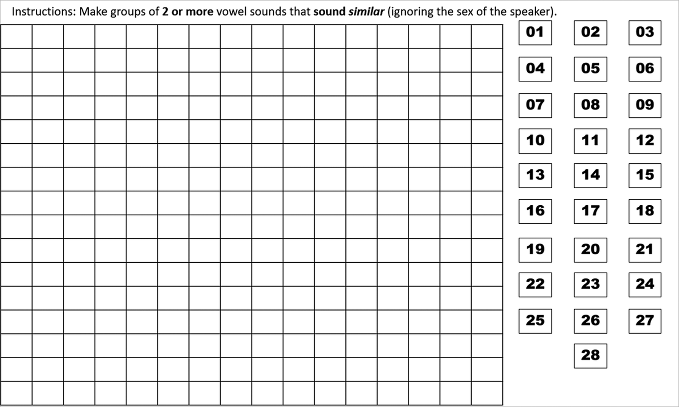
Figure 2. Screenshot of the German free classification task.
Numbers were randomly assigned to the stimuli but remained the same across participants. The alveolar and velar contexts were presented on separate slides. The order of slides was counterbalanced across participants, with half the participants completing the slide with the alveolar context first and the other half completing the slide with the velar context first. Listeners were shown how to click on the stimuli to play the sound files and told to drag each of the items onto the grid to make groups of similar-sounding vowels. Groups had to consist of at least two stimuli, but there was no upper limit on the number of stimuli in a group. Participants could listen to and rearrange the sound files on the grid as many times as they wanted. A screenshot of a slide as completed by a participant is shown in Figure 3. The task was presented on a desktop computer, and participants listened to the stimuli via headphones. The task took around 10 min for listeners to complete.
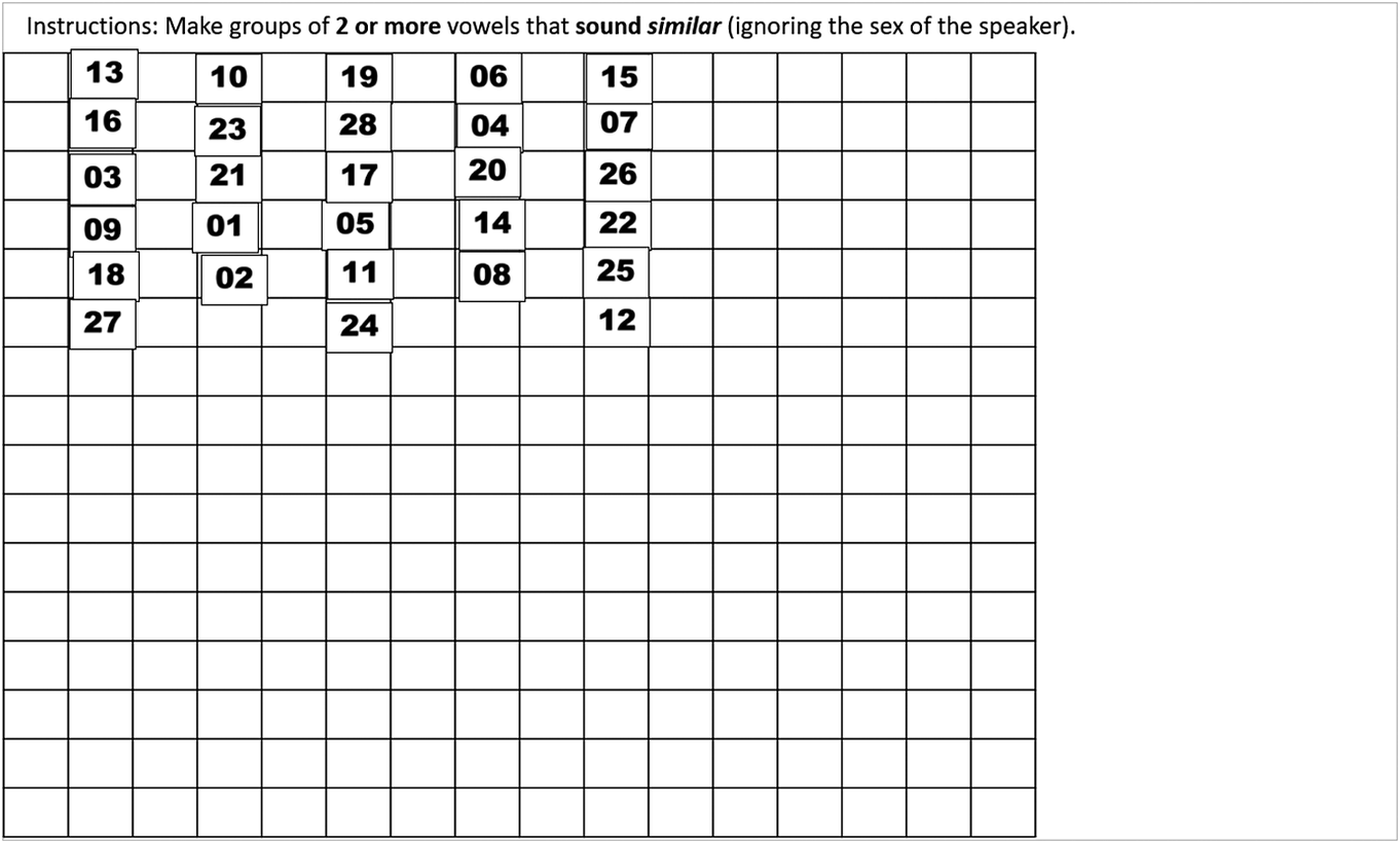
Figure 3. Screenshot of the German free classification task as completed by a participant.
Oddity
An oddity task was used to examine discrimination ability.Footnote 2 In the oddity task, participants heard three stimuli in a row and had to choose which of the three was different or, alternately, that they were all the same. Stimuli from two female speakers and one male speaker were presented in each trial, always in the order female speaker 1, male speaker, female speaker 2. During each trial, participants saw three different colored robots and an X in a row on the screen. Participants indicated which robot “said” something different by clicking on the relevant robot or by clicking on the X following the robots to indicate that all the stimuli were the same.
Eleven German vowel pairs that were expected to vary in discriminability were presented: /u-y/, /u-o/, /y-ø/, /o-e/, /i-e/, /i-a/, /ɪ-ɛ/, /ɪ-ʏ/, /e-ɛ/, /e-a/, and /ø-ʏ/. Each contrast appeared in both the alveolar and velar context. These stimuli pairs appeared once each in the six possible sequences of “different” trials (ABB, BAA, ABA, BAB, AAB, BBA) and twice in each of the two possible “same” trials (AAA, BBB). For example, the [skuk-skyk] stimuli pair appeared twice as [skuk-skuk-skuk] (AAA) and twice as [skyk-skyk-skyk] (BBB), once in the order [skuk-skyk-skyk] (ABB), once in the order [skyk-skuk-skuk] (BAA), and so on. This resulted in 220 trials (11 contrasts × 2 contexts × 10 trial sequences). The interstimulus interval (ISI) in each trial was 400 ms, the intertrial interval (ITI) was 1,000 ms, and the timeout for the trials was set to 3,500 ms. Participants also completed eight training trials with the /o-e/ contrast in the context /bVtə/ to familiarize them with the task. Participants needed to correctly respond to at least six out of eight of the practice trials to proceed to the actual task; otherwise, they repeated the training. The task lasted approximately 20 minutes, with one break in the middle. The two blocks contained an equal number of trials per condition, and trials were randomized within each block. The oddity task was administered through a web browser with jsPsych (de Leeuw, Reference de Leeuw2015).
Procedure
After consenting to participate in the study, the participants completed a bilateral hearing screening, followed by the free classification task and the background questionnaire. Next, they completed the oddity task and, finally, a perceptual assimilation task that is not discussed in the current study.
Participants
The participants were American English speakers recruited from universities in the United States. Their parents were also native speakers of English, and no participant spoke any other language but their native language at home. None had spent more than 3 months in a non-English-speaking country. Additionally, none of the participants spoke or had studied German or another language with front-rounded vowels, and none had taken a linguistics course. In total, 31 participants (22 female; mean age = 19.3 years) were included in the final analyses. All participants included in the final analyses passed the hearing screening and none reported any problems with their hearing, speech, or vision. They also all passed the oddity task training phase and did not have more than 5% timeouts on the test phase of the oddity task.
Analyses and Results Footnote 3
Free Classification Analyses and Results
The first step in analyzing the free classification results was to determine how often participants grouped the different stimuli together. For example, if a participant made a group consisting of all the female and male /y/ tokens as well as the female and male /u/ tokens, then the similarity between /y/ and /u/ would be 100% for that participant. The grouping rates in free classification were calculated for the alveolar and velar contexts separately, as well as both contexts combined. For the combined analysis, the total number of times the stimuli for each vowel pair were grouped together for both consonant contexts was calculated and then divided by the total number of participants multiplied by two (for the two contexts) to yield the percentage of the time the vowels were grouped together. The grouping rates for the combined contexts are given in Table 2.
Table 2. German vowel grouping rates from free classification in percentages

Note. The contrasts examined in the oddity task are bolded and italicized. Groupings of less than 5% are suppressed and percentages are rounded to the nearest whole percentage unless they are one of the oddity contrasts.
As we can see in Table 2, some vowels were never grouped together but others were often grouped together. For example, /o/ and /e/ were never grouped together as similar, but /y/ and /u/ were grouped together nearly 55% of the time. Assuming that vowels that are grouped together as similar more frequently will be harder to discriminate, these grouping rates give us the following predicted order of discriminability for the oddity task, from most difficult to least difficult: /u-y/, /i-e/, /ø-ʏ/, /ɪ-ɛ/, /y-ø/, /e-ɛ/, /u-o/, /ɪ-ʏ/, /e-a/, /i-a/, /o-e/.
In addition to calculating grouping rates, we also performed MDS analyses to visualize the perceptual space and determine what dimensions listeners used to judge perceptual similarity. To conduct the MDS analyses, we created dis-similarity matrices by inverting the percentages for all grouping rates (i.e., 1 – percent score) for the male and female stimuli separately, thus creating a 28 × 28 matrix of how often each stimulus was not grouped with every other stimulus. Male and female tokens were not combined because we could not assume that participants perceived them as the same vowel category. MDS analyses were performed for the alveolar and velar contexts separately, as well as the consonant contexts combined. Following Atagi and Bent (Reference Atagi and Bent2013), the MDS analyses were performed on these data using the ALSCAL function in SPSS 27. We calculated one-, two-, three-, four-, and five-dimensional solutions. To evaluate which was the best fit, for each solution we examined the matrix stress, which indicates the degree of model misfit, and R 2, which gives the amount of variance in the dissimilarity matrix accounted for by the model. Because higher stress in MDS indicates greater model misfit, Clopper (Reference Clopper2008, p. 578) recommends looking for the “elbow” in the stress plot to find the number of dimensions beyond which stress does not considerably decrease, whereas Fox et al. (Reference Fox, Flege and Munro1995, p. 2544) recommend looking for the number of dimensions beyond which R 2 does not considerably increase, provided that this number of dimensions is interpretable based on the relevant theory. Clopper (Reference Clopper2008) also states that a stress value of less than 0.1 for the matrix is considered evidence of “good fit,” although she acknowledges that this is rarely achieved in speech perception data. For these data, there was not a clear elbow in the stress plot but instead a gradual decrease in stress from one to four dimensions. Stress decreased considerably and R 2 increased when moving from a one- to two-dimensional solution and from a two- to a three-dimensional solution, but having four or more dimensions did not reduce stress or increase R 2 much further. Because three dimensions were interpretable and stress decreased below .10 for the three-dimensional solution (e.g., 0.084 for the combined three-dimensional solution versus 0.144 for the combined two-dimensional solution), we decided on the three-dimensional solution for all analyses. We then rotated the solutions to make the most sense graphically while preserving the relative distances between all the stimuli. The rotated solution for the consonant contexts combined is displayed in Figures 4 and 5. To visualize the three-dimensional solution, Figure 4 displays Dimension 1 by Dimension 2 and Figure 5 displays Dimension 1 by Dimension 3 (i.e., as if the viewer were looking down into Figure 4 from the top). Because dimension scores have no inherent meaning and are only important relative to each other, the exact numbers are not indicated along the axes. For each figure, the symbols in black represent the male speaker’s values and the symbols in gray represent the female speaker’s values.

Figure 4. Dimension 1 by Dimension 2 for the rotated German vowel solution with contexts combined.

Figure 5. Dimension 1 by Dimension 3 for the rotated German vowel solution with contexts combined.
In terms of interpreting the solutions, it should be emphasized that MDS does not plot stimuli with respect to any predetermined external criteria, so deciding on the meaning of the dimensions requires a separate analysis. This is typically done by using correlations with stimuli measurements or traits (Clopper, Reference Clopper2008). Because the participants were native speakers of American English, we would expect them to mainly use differences in vowel quality to group the stimuli. However, as free classification does not impose any restrictions on their groupings, it is possible that they used other aspects of the sound files to decide on their similarity. Thus, we included many different properties of the stimuli in our correlational analysis. To determine the acoustic properties of the free classification sound files, these stimuli were acoustically analyzed in Praat (Boersma & Weenink, Reference Boersma and Weenink2019). Total duration of the vowel as well as its F1, F2, F3, f0, and dB values at the halfway point of the vowel’s duration were extracted. Given the inherent variation between voices, formants were normalized according to Gerstman’s formula following Flynn (Reference Flynn2011). Normalized mean F1 and F2 for each vowel are plotted in Figure 6, with the female values again in gray and the male values in black.

Figure 6. Average normalized F1 and F2 of the German stimuli.
Because perceptual similarity of vowels is assumed to vary based on aspects of vowel quality and quantity, we ran Pearson correlations in R with the Hmisc package v4.0-3 (Harrell, Reference Harrell2019) between the rotated dimension scores from the MDS solutions for each individual consonant context and acoustic measurements of our stimuli, specifically vowel duration and the normalized values for F1, F2, and F3. We also included correlations with phonological features of the vowels, specifically (1) roundedness, with 1 for rounded vowels (/y/, /ʏ/, /u/, /ʊ/, /o/, /ɔ/, /ø/, /œ/), 0 for unrounded (/i/, /ɪ/, /e/, /ɛ/), and 0.5 for the two open vowels unspecified for rounding (/a/ and /a:/) and (2) length, with 1 for all phonologically long/tense vowels (/y/, /i/, /u/, /e/, /o/, /ø/, /a:/) and 0 for the phonologically short/lax vowels (/ʏ/, /ɪ/, /ʊ/, /ɛ/, /ɔ/, /œ/, /a/). Finally, to exclude the possibility that listeners were grouping stimuli for reasons other than vowel quality or quantity, we additionally included correlations with intensity (dB), pitch (f0), and speaker sex (coded dichotomously as 1 for female and 0 for male). The resulting Pearson correlations are displayed in Table 3. The p values for these correlations were corrected for multiple comparisons with Benjamini and Hochberg’s false discovery rate (FDR) procedure, at the α = 0.05 level (Benjamini & Hochberg, Reference Benjamini and Hochberg1995). The strongest significant correlation in each row is bolded, italicized, and marked with an asterisk; other significant correlations are also marked with an asterisk.
Table 3. Correlations of MDS rotated dimension scores with acoustic measures and phonological features of German vowel stimuli

Note. Dur refers to vowel duration, Round refers to roundedness, and Phono Length refers to phonological length (tense/lax or long/short). Significant correlations after FDR corrections are marked with an asterisk.
Strong significant correlations were found between Dimension 1 and the acoustic measures of F2 and F3 (both p < .001), but the strongest correlation for Dimension 1 was with roundedness coded as an abstract phonological feature, at r = .962, p < .001. As can be seen in Figure 4, roundedness was more important than vowel backness, with front-rounded vowels grouped together with back-rounded vowels and unrounded front vowels forming their own cluster. For Dimension 2, the strongest significant correlation was with F1, at r = -.801, p < .001, although the correlations with F2 (p < .001) and F3 (p = .003) were also significant. As can be seen in Figure 4, participants grouped stimuli principally by vowel height for Dimension 2, with high vowels such as /i/ and /y/ in the highest positions and low vowels like /a/ and /a:/ in the lowest positions. Finally, Dimension 3 correlated significantly with duration (p = .007) but more strongly with phonological length as an abstract feature, at r = -0.577, p < .001. As shown in Figure 5, for all pairs of long/short (/a:/ and /a/) or tense/lax vowels (e.g., /i/ and /ɪ/), the long/tense vowel was located in a higher position in Dimension 3 than the corresponding short/lax vowel. Pitch, duration, intensity, and speaker sex were not significantly correlated with any dimension.
When comparing the MDS solution to the actual measurements for the German vowels (as seen in Figure 6), the most obvious difference is that /y/, /ʏ/, /ø/, and /œ/ were very close to German back vowels in the MDS solution rather than being more central according to their F2 measurements in acoustic space. The MDS distances among the front unrounded vowels—/i/, /ɪ/, /e/, and /ɛ/—were smaller along Dimensions 1 and 2 than would be expected from their position in the acoustic space, suggesting that these vowels were primarily differentiated from each other in terms of phonological length rather than acoustic differences in F1 and F2.
Oddity Analyses and Results
To determine the utility of free classification for predicting discrimination, we first analyzed performance on the oddity task. Accuracy scores for each of the contrasts were computed, excluding any trials in which participants timed out. Because the data violated the assumptions for a repeated-measures ANOVA, a nonparametric Friedman test was run in R using the rstatix package v.0.3.1 (Kassambara, Reference Kassambara2019) to determine whether the results on the oddity task differed by contrast. For this test, accuracy rate was the dependent variable and contrast (/u-y/, /u-o/, /y-ø/, /o-e/, /i-e/, /i-a/, /ɪ-ɛ/, /ɪ-ʏ/, /e-ɛ/, /e-a/, and /ø-ʏ/) was the independent variable. Results revealed that accuracy rates were significantly different across the contrasts, χ2 (10) = 192.16, p < .001, with a large effect size, W = 0.62. Post hoc pairwise Wilcoxon signed-rank tests were corrected for multiple comparisons with the Bonferroni correction method. These post hoc tests revealed that the following contrasts were not significantly different from each other: /ø-ʏ/, /u-y/, and /y-ø/; /u-y/ and /i-e/; /ɪ-ɛ/, /i-e/, /u-o/, /ɪ-ʏ/, and /e-ɛ/; /u-o/, /ɪ-ʏ/, /e-ɛ/, and /e-a/; /ɪ-ʏ/, /e-ɛ/, /e-a/, and /o-e/; and /e-a/, /o-e/, and /i-a/. All other contrasts were significantly different from each other at an adjusted alpha level of .05. Figure 7 displays the results for the oddity task, ordered by the contrast with the lowest mean accuracy to the contrast with the highest mean accuracy. Diamonds indicate mean values. Curly brackets encompass groups of contrasts that were not significantly different from each other. The square bracket represents that only those two contrasts, but not the contrasts between them, were not significantly different from each other.

Figure 7. Oddity results by contrast for German vowels.
Comparison Between Free Classification and Oddity Results
To determine how well the free classification results predicted the accuracy of the contrasts in oddity, linear regressions were run in R using the lm function of the built-in stats package in R version 4.0.2 (R Core Team, 2020) and tables were created in part with the apaTables package v.2.0.5 (Stanley, Reference Stanley2018). For both analyses, results were divided by contrast as well as context (alveolar and velar). Because all of the voices were presented against each other in the oddity task, we first averaged the grouping rates (or MDS distances) for each contrast in the free classification task across the male and female tokens to obtain average similarity rates for all pairs of phonemes. For example, in the alveolar context, male /i/ was grouped with male /ɪ/ at a rate of 3.2%, male /i/ with female /ɪ/ at 6.5%, female /i/ with female /ɪ/ at 12.5%, and female /i/ with male /ɪ/ at 9.7%. This gave an average similarity rate of 7.98% for /i-ɪ/ in the alveolar context. In the first regression analysis, the raw free classification similarity rates served as the independent variable and the oddity accuracy scores as the dependent variable. This regression equation was significant, F(1, 20) = 32.97, p < .001, showing that free classification similarity rates predicted performance on the oddity task. Table 4 displays a summary of this analysis.
Table 4. Regression analysis of German oddity with free classification similarity rates as predictor

Note. B = unstandardized regression weight. r = zero-order correlation, which is identical to the standardized regression weight. Numbers in brackets indicate the lower and upper limits of a bootstrapped 95% confidence interval.
The strong negative correlation of r = -.79, which is the same as the standardized regression weight, shows that as free classification similarity rates increased, accuracy in oddity decreased. This indicates that the more similar the two sounds of a contrast were perceived to be, the harder they were to discriminate.
Next, an analysis was conducted with the distances produced by the MDS solution to determine whether these distances better predicted discriminability compared with the raw free classification similarity rates. Euclidean distances were calculated between all of the points produced by the MDS analysis for the contrasts present in the oddity task. These distances served as the independent variable in a regression analysis, with oddity scores as the dependent variable. This analysis also produced a significant regression equation, F(1, 20) = 23.83, p < .001, as summarized in Table 5.
Table 5. Regression analysis of German oddity with MDS distances as predictor

Note. B = unstandardized regression weight. r = zero-order correlation, which is identical to the standardized regression weight. Numbers in brackets indicate the lower and upper limits of a bootstrapped 95% confidence interval.
The strong positive correlation, r = .74, shows that as MDS distance increased—that is, as sounds were perceived as more distinct—accuracy in oddity increased. Comparing the results from the regression analyses examining free classification similarity rates and MDS distances, free classification similarity was a slightly better predictor of oddity discrimination accuracy for the German vowel experiment.
Discussion
Free classification similarity rates predicted the following order of difficulty, from most to least difficult: /u-y/, /i-e/, /ø-ʏ/, /ɪ-ɛ/, /y-ø/, /e-ɛ/, /u-o/, /ɪ-ʏ/, /e-a/, /i-a/, and /o-e/. These predictions corroborate previous studies that demonstrated high difficulty for /u-y/, pairs of front-rounded vowels (/ø-ʏ/ and /y-ø/), and /i-e/ (e.g., Darcy et al., Reference Darcy, Daidone and Kojima2013; Kingston, Reference Kingston2003). In our oddity task, we similarly observed that /ø-ʏ/, /u-y/, and /y-ø/ were difficult to discriminate. Free classification similarity rates also correctly predicted that /e-a/, /o-e/, and /i-a/ would be the least difficult contrasts. In general, contrasts differing in backness but not roundedness were the most difficult for listeners, as expected from previous literature showing that front-rounded vowels assimilate to back-rounded vowels in English (e.g., Strange et al., Reference Strange, Bohn, Nishi and Trent2005). However, free classification overpredicted the difficulty of /i-e/, /ɪ-ɛ/, and /e-ɛ/ (though /i-e/ was not significantly different from /u-y/ in oddity). This suggests that free classification is useful in predicting discriminability but may overpredict the discriminability of contrasts that contain sounds that are quite similar perceptually but at the same time have separate phonemic equivalents in the L1. Nevertheless, the regression analyses show that free classification was useful in predicting the discriminability of German vowel contrasts, with strong correlations between raw similarity rates and performance in oddity, as well as between the MDS distances and performance in oddity, although to a lesser degree. The MDS dimension scores and their correlations with acoustic, phonological, and indexical properties of the stimuli separately provided data on what dimensions listeners pay attention to when perceiving these vowels. For these American English listeners, roundedness, F1, and phonological length were the most important properties of the stimuli in determining the similarity of German vowels. These findings are not surprising given that English vowels are also distinguished by F1 (height) and phonological length (tense/lax) and that roundedness rather than backness has determined the mapping of German vowels to English vowels in previous studies (i.e., front-rounded vowels are assimilated to back-rounded vowels instead of front-unrounded vowels). Nevertheless, using free classification has made it possible to empirically demonstrate that these are the most important factors in American English listeners’ perception of German vowels.
Experiment 2: Finnish Phonemic Length
The main advantage of a free classification task is that it can be used just as easily for examining suprasegmental phenomena. In Finnish, both vowels and consonants can be long or short. For example, tuli means “fire,” but tuuli with a long /u/ means “wind,” and tulli with a long /l/ means “customs.” For two-syllable words of the form CVCV, there are eight combinations of short and long segments that are phonotactically possible: CVCV, CVVCV, CVCCV, CVCVV, CVVCVV, CVCCVV, CVVCCV, CVVCCVV, where double letters indicate a long segment. Previous research on the acquisition of Finnish length has been limited to the comparison of a word with no long segments to one with a single long segment (e.g., CVCV vs. CVCCV in Porretta & Tucker, Reference Porretta and Tucker2014, or CVCV vs. CVVCV in Ylinen et al., Reference Ylinen, Shestakova, Alku and Huotilainen2005). Thus, little is known about the degree of confusion among forms with one or more long segments and nearly nothing about the factors involved. Studies on other languages with quantity contrasts have shown that, in general, initial vowel length contrasts tend to be more easily discriminated than consonant length (Altmann et al., Reference Altmann, Berger and Braun2012; Hirata & McNally, Reference Hirata and McNally2010) and final vowel length is typically harder to discriminate than vowel length contrasts in other positions (Minagawa et al., Reference Minagawa, Maekawa and Kiritani2002); however, most combinations of length have not been tested to date. In other languages, vowel quality is known to interact with quantity distinctions, but it is unclear whether or not that would be the case for Finnish or what other cues would be employed by learners. One possible explanation for the lack of research on this topic is that it is not clear how a PA task could be developed or interpreted for listeners with a language without phonemic length. Using a free classification task allowed us to examine the perception of length templates, such as CVCV vs. CVVCV, rather than individual short and long vowels and consonants and compare their perceptual similarity with discrimination results from an oddity task. American English listeners were tested to investigate the effectiveness of free classification for predicting the discriminability of a suprasegmental feature that does not exist in participants’ L1 as a principal cue to lexical differences.
Stimuli
All eight length templates possible in Finnish disyllabic words were included for the contexts pata, tiki, and kupu. For example, the full range of pata stimuli was [pata], [paata], [patta], [pataa], [paataa], [pattaa], [paatta], and [paattaa]. Three female native speakers of Finnish from Helsinki were recorded for all of the stimuli. The first speaker, an instructor of Finnish language, judged the stimuli to be target-like.
Tasks
Free Classification
As in the German experiment, the free classification task was administered via a PowerPoint presentation which contained a 16 × 16 grid on the left and numbered sound files on the right. Participants completed three slides that each contained the eight length templates for a context (pata, tiki, or kupu) spoken by each of the three speakers, resulting in 24 stimuli per slide. These stimuli were randomly assigned the numbers 1–24. The instructions on each slide directed participants to “make groups of 2 or more words that sound similar based on how long the vowels and consonants in each word sound to you. (Ignore differences in speaker and intonation).” This task took 15–20 min to complete.
Oddity
The oddity task for Finnish length was nearly identical in design to the oddity task for the German experiment. Participants heard three stimuli in a row and clicked on a robot to indicate which word was different or on the X to indicate that the stimuli were all the same. The three female speakers were always presented in the same order during a trial such that each robot always corresponded to the same voice. Eight length contrasts were tested: (1) CVCV-CVCCV, (2) CVCV-CVVCV, (3) CVCCV-CVVCV, (4) CVVCV-CVCVV, (5) CVCCVV-CVVCVV, (6) CVVCV-CVVCCV, (7) CVVCVV-CVVCCVV, and (8) CVVCCV-CVVCCVV. Each of these contrasts appeared in the three contexts pata, tiki, and kupu, and each contrast appeared once in the six possible sequences of “different” trials (ABB, BAA, ABA, BAB, AAB, BBA) and twice in each of the two possible “same” trials (AAA, BBB). For example, the [kupu-kuppu] stimuli pair appeared twice as [kupu-kupu-kupu] (AAA) and twice as [kuppu-kuppu-kuppu] (BBB), once in the order [kupu-kuppu-kuppu] (ABB), once in the order [kuppu-kupu-kupu] (BAA), and so on. This resulted in 240 trials examining length (8 contrasts × 3 contexts × 10 trial sequences). We also added a block of a control segmental contrast, /i-a/, to the beginning of the task to verify that the task was doable for the participants. If participants performed poorly on the length contrasts but performed near ceiling on the segmental contrast, we could attributed their performance to the nature of those contrasts rather than a misunderstanding of the task itself. This brought the total number of trials to 260. Stimuli were blocked by contrast, resulting in one block of 20 stimuli for the segmental contrast and eight blocks of 30 stimuli for the length contrasts. Stimuli were randomized within blocks and breaks were provided between each block. The ISI in each trial was 400 ms, the ITI was 1,000 ms, and the timeout was 2,500 ms. Like the German experiment, participants also completed eight training trials with the /o-e/ contrast. The task lasted approximately 20 min and was administered through a web browser with jsPsych.
Procedure
After participants gave their consent, they completed a bilateral hearing screening. This was followed by the free classification task, the oddity task, and a background questionnaire. Participants then completed an identification task that is not reported on in the current study.
Participants
For the Finnish experiment, American English listeners with no knowledge of Finnish were tested. The American English listeners were recruited from a large Midwestern university and consisted of 26 participants (20 female; mean age = 19.0 years). None of the participants spoke or had studied another language with phonemic length, none had spent more than 3 months in a non-English-speaking country, and none had taken a linguistics course. Participants’ parents were also native speakers of English, and no participant spoke any other language but their native language at home. All of the participants that completed this experiment were different individuals from those that completed Experiment 1. The participants included in the final analyses passed the hearing screening, and none reported any problems with their hearing, speech, or vision. They also all passed the oddity task training phase and did not have more than 5% timeouts on the test phase.
Analyses and Results Footnote 4
Free Classification Analyses and Results
Following the same procedure as for the German vowel experiment, grouping rates were calculated for the free classification task. The results for all contexts combined (pata, tiki, and kupu) are displayed in Table 6. As we can see, all length templates were grouped with each other over 6% of the time, suggesting that participants found most length templates to be similar to at least some degree. These grouping rates gave us the following predicted order of discriminability for the oddity task, from most difficult to least difficult: (1) CVVCV-CVVCCV, (2) CVCV-CVCCV, (3) CVVCVV-CVVCCVV, (4) CVVCCV-CVVCCVV, (5) CVCCVV-CVVCVV, (6) CVCCV-CVVCV, (7) CVVCV-CVCVV, and (8) CVCV-CVVCV. In general, contrasts that involve a consonant-length distinction were predicted to be most difficult, whereas contrasts that involve a distinction in initial vowel length were predicted to be easiest.
Table 6. Finnish length grouping rates from free classification in percentages

Note. The contrasts examined in the oddity task are bolded and italicized. Percentages are rounded to the nearest whole percentage unless they are one of the oddity contrasts.
MDS analyses were run on the data for the pata, tiki, and kupu contexts separately as well as these contexts combined. We decided on a three-dimensional solution for all analyses because stress fell under .20 for the three-dimensional versus above .20 for the two-dimensional solution in all cases and an elbow in the stress plot was clear at three dimensions for the tiki, kupu, and combined plots. Although ideally stress would be under .10, this was only achieved with the five-dimensional solution in each context, which would be difficult to interpret. Thus, we chose a three-dimensional solution as the best compromise between model fit on the one hand and interpretability and imageability on the other. The rotated solution for the combined analysis is displayed in Figures 8 and 9. Figure 8 displays Dimension 1 by Dimension 2, and Figure 9 displays Dimension 1 by Dimension 3 (i.e., as if the viewer were looking down into Figure 8 from the top). For each figure, the symbols in black represent Speaker 1, symbols in gray represent Speaker 2, and symbols in white represent Speaker 3.

Figure 8. Dimension 1 by Dimension 2 for the rotated Finnish length solution with contexts combined.

Figure 9. Dimension 1 by Dimension 3 for the rotated Finnish length solution with contexts combined.
Because the participants were asked to make groups based on how long the vowels and consonants in each word sounded, we hoped they would use length to group the stimuli, particularly initial vowel length given the previous literature on length perception. Nevertheless, as American English does not have phonemic length, it was also probable that they used other properties of the stimuli, such as vowel quality, to group the sound files. Consequently, we included many different aspects of the stimuli in the correlational analysis with dimension scores. The Finnish stimuli were acoustically analyzed in Praat to determine the acoustic properties of the stimuli. Properties of the initial consonant (C1), the first vowel (V1), the second consonant (C2), and the second vowel (V2) were analyzed. Specifically, we measured the duration of C1 voice onset time (VOT), duration of V1, the closure duration of C2, the duration of C2 VOT, and the duration of V2, as well as overall duration. Figure 10 displays the mean length of each of these measurements by length template for the three speakers, averaged across the pata, tiki, and kupu contexts, although the individual values were used in the correlational analysis. The F1, F2, and F3 of V1 and V2 at the halfway point of each vowel’s duration were also calculated. Following the procedure for the German analysis, formants were normalized across speakers according to Gerstman’s formula. Finally, average f0 and average dB values were extracted for each stimulus.

Figure 10. Average length of segments in the Finnish stimuli.
We ran Pearson correlations in R with the Hmisc package v4.0-3 (Harrell, Reference Harrell2019) between the rotated dimension scores for each context and acoustic measurements of our stimuli, specifically C1 VOT duration, V1 duration, C2 closure duration, C2 VOT duration, V2 duration, V1 minus V2 duration, overall duration, normalized values for F1, F2, and F3, and average dB and f0. We also included correlations with phonological length for V1, C2, and V2 and the difference in phonological length between V1 and V2, with 1 for long segments and 0 for short segments. The results of the correlational analysis are displayed in Table 7. The p values for these correlations were corrected for multiple comparisons with Benjamini and Hochberg’s (Reference Benjamini and Hochberg1995) false discovery rate (FDR) procedure, at α = 0.05. The strongest significant correlation for each dimension is bolded, italicized, and marked with an asterisk; other significant correlations are also marked with an asterisk.
Table 7. Correlations of MDS rotated dimension scores with acoustic measures and phonological features of Finnish length stimuli

Note. Length refers to phonological length (short or long), Dur refers to duration, and Avg refers to average. Significant correlations after FDR corrections are marked with an asterisk.
Dimension 1 correlated most strongly with V1 length as an abstract phonological feature, at r = .752, although it also correlated with the duration of V1, overall word duration, and the V1 minus V2 phonological length difference (all p < .001). As can be seen in Figure 8, stimuli with a short V1 tend to appear to the left side of Dimension 1, whereas stimuli with a long V1 tend to appear to the right side. Dimension 2 correlated most strongly with V2 duration, at r = -0.779, p < .001. It also correlated with V2 length as a phonological feature, V1 minus V2 duration, the V1 minus V2 phonological length difference, and overall word duration (all p < .001). Although Dimension 2 does not separate the stimuli as well as Dimension 1, in Figure 8 we can see that short V2 stimuli are mainly higher in Dimension 2 than long V2 stimuli. For Dimension 3, V1 minus V2 duration was the strongest significant correlation, at r = .353, p = .002. It also correlated with the V1 minus V2 phonological length difference (p = .003), V1 phonological length (p = .003), and V1 duration (p = .004). No other correlations were significant, specifically any of the consonant measures, pitch, or intensity. Thus, it appears that participants grouped the stimuli primarily according to the phonological length/duration of the vowels.
Oddity Analyses and Results
Participants’ scores on the control segmental contrast (/i-a/) confirmed that they understood the task (M = .976, SD = .04). Accuracy scores for each of the length contrasts were computed with the contexts combined, excluding any trials in which participants timed out. A repeated-measures ANOVA was run in R using the rstatix package v.0.3.1 (Kassambara, Reference Kassambara2019), with oddity accuracy rate as the dependent variable and contrast (CVCV-CVCCV, CVCV-CVVCV, CVCCV-CVVCV, CVVCV-CVCVV, CVCCVV-CVVCVV, CVVCV-CVVCCV, CVVCVV-CVVCCVV, CVVCCV-CVVCCVV) as the independent variable. The data were judged to be approximately normally distributed when examining the QQ plots of the data, and Mauchly’s test of sphericity showed that the assumption of sphericity was also met (p = .06). The results of the ANOVA revealed that accuracy rates were significantly different across contrasts, F(7, 175) = 35.651, p < .001, with a large effect size, η2 G = 0.43. Post hoc pairwise t tests were corrected for multiple comparisons with the Bonferroni correction method, revealing that the following contrasts were not significantly different from each other: CVVCVV-CVVCCVV and CVVCV-CVVCCV; CVVCV-CVVCCV, CVVCCV-CVVCCVV, and CVCCVV-CVVCVV; CVVCCV-CVVCCVV, CVCCVV-CVVCVV, and CVCV-CVCCV; CVCV-CVCCV and CVVCV-CVCVV; CVCCV-CVVCV, CVVCV-CVCVV, and CVCV-CVVCV. All other contrasts were significantly different from each other at an adjusted alpha level of .05. Figure 11 displays the results for the oddity task, ordered by the contrast with the lowest mean accuracy to the contrast with the highest mean accuracy. Diamonds indicate mean values. Curly brackets encompass groups of contrasts that were not significantly different from each other. The square bracket represents that only those two contrasts, but not the contrast between them, were not significantly different from each other. In general, consonant contrasts were the most difficult, whereas contrasts containing a difference in the first vowel were the easiest.

Figure 11. Oddity results by contrast for Finnish length.
Comparison Between Free Classification and Oddity Results
To determine how well the free classification task predicted the accuracy of the contrasts in oddity, results for each length contrast were divided by context (pata, tiki, kupu) for both the oddity and free classification tasks, yielding 24 average oddity scores and 24 overall free classification similarity rates (eight length contrasts × three contexts). A linear regression was then run in R, with oddity scores as the dependent variable and free classification similarity rates as the independent variable, yielding a significant regression equation, F(1, 22) = 15.68, p < .001. Table 8 displays a summary of this analysis.
Table 8. Regression analysis of Finnish oddity with free classification similarity rates as predictor

Note. B = unstandardized regression weight; r = zero-order correlation, which is identical to the standardized regression weight. Numbers in brackets indicate the lower and upper limits of a bootstrapped 95% confidence interval.
The regression analysis showed that free classification similarity rates were a significant predictor of oddity discrimination accuracy. The strong negative correlation, or standardized regression weight, indicates that as free classification similarity rates increased, discriminability in oddity decreased, r = -.65. In other words, the greater the perceived similarity of two stimuli, the harder they were to discriminate. To see whether the distances that were produced by the MDS solution better predicted discriminability compared with the raw free classification similarity rates, Euclidean distances were calculated between all of the points for the contrasts present in the oddity task, divided by context (pata, tiki, kupu). A linear regression with oddity scores as the dependent variable and MDS distances as the independent variable also yielded a significant regression equation, F(1, 22) = 49.5, p < .001. A summary of this analysis is displayed in Table 9.
Table 9. Regression analysis of Finnish oddity with MDS distances as predictor

Note. B = unstandardized regression weight; r = zero-order correlation, which is identical to the standardized regression weight. Numbers in brackets indicate the lower and upper limits of a bootstrapped 95% confidence interval.
The regression analysis revealed that MDS distances significantly predicted oddity discriminability. The very strong positive correlation shows that as MDS distance increased, accuracy in oddity increased, r = .83. When the analyses for free classification similarity rates and MDS distances are compared, MDS distances are a better predictor of oddity discrimination accuracy.
Discussion
In general, the discrimination results for Finnish are in line with previous findings for quantity contrasts in other languages—namely, vowel differences, and especially initial vowel length contrasts, were easier to discriminate than consonant contrasts. As mentioned, however, most length contrasts have not yet been investigated, so the ability of free classification to predict discrimination difficulty is a crucial test of its utility. According to the free classification similarity rates, we predicted the following order of difficulty in discriminating Finnish length contrasts, from most to least difficult: (1) CVVCV-CVVCCV, (2) CVCV-CVCCV, (3) CVVCVV-CVVCCVV, (4) CVVCCV-CVVCCVV, (5) CVCCVV-CVVCVV, (6) CVCCV-CVVCV, (7) CVVCV-CVCVV, and (8) CVCV-CVVCV. Taking into account which contrasts did not significantly differ from each other in oddity, this prediction was accurate with the sole exception of CVCV-CVCCV, which was predicted to be the second-most difficult but was actually the third-most difficult, with CVVCVV-CVVCCVV surpassing it in difficulty. In addition, regression analyses showed that the free classification results were able to predict performance on the oddity task, with a strong correlation between similarity rates and oddity accuracy and an even stronger correlation between MDS distances and oddity accuracy. Thus, despite the MDS solution not being easily visually interpretable, especially for Dimension 3, these distances predicted discriminability quite well. Additionally, the analysis between MDS dimension scores and acoustic, phonological, and indexical properties of the stimuli revealed that American English listeners were sensitive to vowel length but not consonant length when deciding on the similarity of stimuli, again in line with previous research on other languages, and this appears to be reflected in the oddity results as well.
Overall Discussion
According to Flege (Reference Flege and Wayland2021), L2 speech research methodology “has received relatively little attention in recent years” and “the lack of attention to methodology […] has slowed progress in the field and resulted in a heterogeneity of research findings that are difficult to interpret” (p. 119). In this study, we sought to add a new tool to the speech researcher’s toolbelt with the adaptation of free classification tasks to the examination of nonnative perception.
If a free classification is employed, there are important design considerations to take into account. First, it is preferable to include all related sounds as stimuli in the task. For example, when examining vowel perception, it is best to include all the vowels in that language. If not, an MDS analysis and correlations with properties of the stimuli may be difficult to interpret because listeners may not have used all of the relevant dimensions to group the stimuli. Including only front vowels, for instance, may make it falsely seem that vowel backness is not a relevant dimension for grouping vowels. A separate consideration is participant task demand: having a large number of stimuli on screen greatly increases the memory load of comparisons, and presenting more than about 30 stimuli at once would likely exceed the memory capacity of several participants. This restriction on the number of stimuli per slide can be a limitation depending on the phenomenon under investigation. For example, we were only able to include two of the three speakers in the German free classification task because including all three speakers on a slide for the 14 vowels would have resulted in 42 stimuli for the participants to group, which would have been too cognitively demanding. Apart from limiting the number of speakers that can be used, the constraint on the number of stimuli on a slide could make it impossible to include all related sounds. For example, examining all the consonants of a language at once would not be possible with this method and including only a subset could obscure some dimensions that participants would use to group the stimuli. Finally, researchers examining individual differences in perception would find free classification less than optimal because the data provided on an individual level is less fine grained than other tasks such as similarity judgments or perceptual assimilation tasks.
With those caveats in mind, our findings show that free classification tasks are a promising method for future research. These tasks are quicker to complete than a traditional similarity judgment task but can provide rich data on the perceptual dimensions that participants use to group stimuli. To illustrate, by comparing free classification results with phonological and acoustic traits of the stimuli, we found that roundedness, F1, and phonological length were the most important factors in American English listeners’ perception of German vowels and the length of the vowels was the most important factor in their perception of Finnish length templates. Moreover, consonant length was essentially ignored by participants in grouping Finnish stimuli in free classification, and on the oddity task, consonant length contrasts were consistently the hardest, which is a potentially important finding for both theorists and language teachers.
Reporting free classification results as grouping rates or calculated MDS distances allows us to use these results to statistically test their accuracy in predicting discrimination rather than making qualitative judgments on their predictive power. This is especially useful because the difficulty of a discrimination task depends on the characteristics of the task used (e.g., Oddity vs. AXB; 500- vs. 1,000-ms ISI; see Strange & Shafer, Reference Strange, Shafer, Edwards and Zampini2008), and therefore subjectively characterizing discrimination performance in terms of descriptors like “good” or “poor,” as has traditionally been done when comparing discrimination results to the categorical results of a PA task, presents difficulties in replicability. Although around 30 participants are needed for the calculation of MDS distances, raw grouping rates could also be analyzed for a smaller subset of participants or at an individual level.
When we analyzed the predictability of free classification results for German vowels and Finnish length, we found that they were good predictors of oddity discrimination accuracy. For German vowels, free classification results were able to predict either 62% or 54% of the variance in oddity scores, depending on whether raw similarity rates (r = -.79) or MDS distances (r = .74) were used. For Finnish length, similarity rates predicted 42% of the variance (r = -.65) and MDS distances 69% of the variance in oddity scores (r = .83). For German vowels the free classification grouping rates were the better predictor of discriminability in oddity, whereas for Finnish length the MDS distances were a stronger predictor. This may be because length was difficult for American English participants to operationalize and the MDS analysis reduced noise in their results from their potential use of idiosyncratic dimensions to group the stimuli. Future studies are needed to determine whether MDS distances are generally stronger predictors for phenomena not present in the listeners’ native language.
Overall, we found that free classification tasks can be used to quantitively predict discriminability. These tasks allow researchers to test a large range of sounds at once and generate a complete similarity matrix for all possible sound pairings (e.g., Table 2). These similarity matrices can then be examined to determine which contrasts are likely to pose difficulties for learners. This technique is in line with the conclusions of Harnsberger (Reference Harnsberger2001a), who states in his abstract that “the discriminability of non-native contrasts is a function of the similarity of non-native sounds to each other in a multidimensional, phonologized perceptual space.”
Additionally, free classification tasks are easily replicable because they do not rely heavily on researcher decisions. Because there is no labeling involved, the decisions necessary for a PA task (what categorization threshold to use, how many categories to present, and how to label these categories) are absent. This makes comparisons across studies easier and works toward reducing the difficulty of interpreting diverse findings in the field as lamented by Flege (Reference Flege and Wayland2021). The lack of labeling not only allows for greater replicability but also entails that these tasks can easily be used to test the perception of segmental and suprasegmental phenomena alike. Although we included only nonnative sounds in both of our experiments, there is no reason that free classification could not also be used to examine the perceptual similarity between L1 and nonnative sounds (i.e., sounds in a language unknown to the participants) or between L1 and L2 sounds (i.e., sounds in a language the participants are learning), depending on the type of phenomenon under investigation.
In summary, free classification tasks are versatile, easily replicated, and as our experiments suggest, strongly predictive of performance on discrimination tasks. We conclude that free classification tasks are a powerful tool for the study of nonnative and L2 perception that could increase researchers’ ability to develop theory and inform teaching practice.
Data Availability Statement
The experiment in this article earned Open Data and Open Materials badges for transparent practices. The materials and analyses for all tasks for both experiments are available at https://osf.io/g3a89/.


 Open access