


Introduction
The recent evolution of the most advanced economies share a clear pattern: a downturn in economic growth rates and a growing process of tertiarisation compared to the so-called Golden Age period. Globalisation, which has been accentuated since the thrust of emerging economies, might explain this structural change in developed economies. The United States (US) is the most remarkable example of this process (Manera Reference Manera2013).
A conjunction of downward phases in cycles of capitalism characterises depression. Every depression has come when the cycle in clusters of innovation has matured and become ‘saturated’; when world production and commodity prices enter a downward phase (inflation slows and even turns into deflation); when the cycle of construction and infrastructure investment has slumped; and above all, when the cycle of profitability is in a downward phase (Roberts Reference Roberts2022, 17). According to this definition of depression, the US has experienced depression since the 1980s, because since then the country has not recovered its previous trend rate of growth. Above all, it means that the profitability of the US domestic capitalist sectors has remained lower.
Another empirical regularity observed in developed economies is the decreasing trend of the profit rate over the last sixty years. Recent works, such as Basu et al (Reference Basu, Huato, Jauregui and Wasner2022), Manera et al (Reference Manera, Navinés, Franconetti and Pérez-Montiel2019b, Reference Manera, Navines, Perez-Montiel and Franconetti2022), and Lapavitsas (Reference Lapavitsas2013), assert that this decrease in the profit rate is mainly explained by the fall of the output-capital ratio (GDP/K), which we will refer to as capital productivity (Manera et al Reference Manera, Navinés and Franconetti2019a; Manera et al Reference Manera, Navines, Perez-Montiel and Franconetti2022b). However, which has been the leading cause of the decrease in capital productivity? Basu et al (Reference Basu, Huato, Jauregui and Wasner2022) state that this fall is related to the increasing tertiarisation of the economy. We aim to contribute to the literature through the characterisation of four aspects of the US economy:
-
The increase in competition between capitals due to the liberalisation and the increasing globalisation of markets (Pariboni Reference Pariboni2016; Pérez-Montiel and Manera Reference Pérez-Montiel and Manera2020) has been key to containing industrial prices. At the same time, it has led to higher competition. Higher competition has led US firms to maintain investment rates.
-
The implementation of restrictive and anti-Keynesian monetary policies, at least until 2008, to control and reduce the high inflation rates of the 1970s (Blanchard et al Reference Blanchard, Romer, Spence and Stiglitz2012; Kim and Allmang Reference Kim and Allmang2021; Haluska Reference Haluska2022; Ghosh Reference Ghosh2023).
-
The service sector’s greater sophistication and diversification thanks to the new ICT technological revolution and the Knowledge Economy (Tridico and Pariboni Reference Tridico and Pariboni2018; Pariboni et al Reference Pariboni, Paternesi Meloni and Tridico2020)
-
The dominance of the financial capital over the productive and industrial ones (Freeman Reference Freeman2010; Roberts Reference Roberts2016, Reference Roberts2022; Hellwig Reference Hellwig2021).
We will argue that these four factors are causally interrelated and are critical to understanding the decreasing trend in capital productivity experienced by the United States in the last decades.
Our research aims to analyse the long-lasting switch experienced by the US economy since the 1970s (Borsato Reference Borsato2023). We argue that increasing globalisation has led to a progressive increase in imports and an increasing external deficit. This denotes a loss of the US resident firms’ foreign and domestic market shares. This is explained by the replacement of domestic production of high-end goods by products imported mainly from the European Union (e.g., automobiles and manufactured goods of prestigious brands) and low-priced consumer goods by products imported from China and other Asian countries. This, along with a more restrictive monetary policy, has made it possible to reduce the high inflation rates of the 1970s and 1980s; at the same time, significant growth in credit to families and companies has facilitated US mass consumption. On the other hand, increasing foreign competition has stimulated investment, which has led to an increasing productive capacity. This greater productive capacity, together with the loss of domestic and foreign market shares, has prevented US resident firms from maintaining their ‘normal’ degree of productive capacity utilisation. Finally, the decline in the degree of capacity utilisation explains the fall in capital productivity.
Our paper contributes to the debate on the declining trend in capacity utilisation in the United States economy (Bansak et al Reference Bansak, Morin and Starr2007; Pierce and Wisniewski Reference Pierce and Wisniewski2018; Gahn Reference Gahn2020). Gahn (Reference Gahn2023) tries to find an explanation for the declining trend in the degree of effective productive capacity utilisation (proxied by the output-capital ratio, which we call capital productivity) and concludes that: ‘There is a declining trend in effective capacity utilisation in the US and there is still no precise answer to this phenomenon’. Gahn finds that shocks to the level of production, distribution, productive technique, and inventories do not have persistent effects on the output-capital ratio. Therefore, our work offers a possible explanatory hypothesis for this enigma in the US.
On the other hand, our work offers an interpretation of the behaviour of the US rate of profit within a critical approach to neoliberal globalisation. In this sense, our paper can be read through the lens of Michael Roberts’ approach: in a context of falling returns on invested capital, the efforts to maintain the rate of profit lay on pressure on the labour force, with different manifestations: cuts in public spending, elimination of social rights, greater labour intensity, new labour-saving technologies, and privatisations. This might explain the increasing gap between growth in labour productivity and wages since the 1970s (Pensiero Reference Pensiero2022). Thus, Roberts (Reference Roberts2016) does not believe that Keynesian postulates would contribute to solving the problems of the US economy. He attributes the economic performance of the ‘glorious thirty years’ to the consequences of the Second World War when the United States put all its productive machinery to boost its economy. The solution to the main economic problems proposed by the author focuses on a way out that he qualifies as ‘socialist’: that governments take charge of the main sectors of the economy to produce for social needs instead of doing it for profit. The central derivative of it would be controlling investments and the ownership of the major banks and other large companies. This, for Roberts, is very different from Keynesian proposals. This argument also aligns with those who claim that industrial policy should be brought back to the front and play a key role in economic policy (Portella-Carbó and Dejuán Reference Portella-Carbó and Dejuán2019; Nieto et al Reference Nieto, Carpintero, Miguel and de Blas2020).
We organise the work as follows. Section two highlights the relationship between the degree of productive capacity utilisation, capital productivity, and the foreign sector. Section 3 empirically tests the relationship between the three mentioned variables, while Section 4 discusses the results. Finally, Section 5 concludes.
Degree of productive capacity utilisation, capital productivity, and the foreign sector
In this section, we demonstrate the dynamic relationship between the imports/GDP ratio ( ${\rm{m}}$
), the degree of utilisation of productive capacity (
${\rm{m}}$
), the degree of utilisation of productive capacity ( ${\rm{u}}$
), and capital productivity (
${\rm{u}}$
), and capital productivity ( ${\rm{\pi k}}$
) in the United States between 1947 and 2020. Due to data availability, we use the data of the non-financial sector to construct capital productivity (GDP/K). On the other hand, we use the series of capacity utilisation corresponding to the manufacturing sector since available data for the series of the total industry starts in 1967. The remarkably high correlation between these two series, which reaches 99% (Graph 1), supports this choice.
${\rm{\pi k}}$
) in the United States between 1947 and 2020. Due to data availability, we use the data of the non-financial sector to construct capital productivity (GDP/K). On the other hand, we use the series of capacity utilisation corresponding to the manufacturing sector since available data for the series of the total industry starts in 1967. The remarkably high correlation between these two series, which reaches 99% (Graph 1), supports this choice.

Graph 1. Degree of productive capacity utilisation in the United States. Manufacturing sector and total industry, 1945–2020. Source: Own elaboration with Federal Reserve Bank of St. Louis data.
Graph 2 plots the series of ${\rm{u}}$
and
${\rm{u}}$
and ${\rm{\pi k}}$
of non-financial US firms: both series share a decreasing trend, although
${\rm{\pi k}}$
of non-financial US firms: both series share a decreasing trend, although ${\rm{u}}$
shows more significant variability than
${\rm{u}}$
shows more significant variability than ${\rm{\pi k}}$
. The Pearson correlation coefficient between them is 76.8%. We can see that between 1948 and 1968, the Keynesian regulation phase, the differences between the series remained relatively steady, with capital productivity being above capacity utilisation until the oil shock of 1973. The period 1950–1968 also experienced the full effects of the Treaty of Detroit (See Armstrong et al (Reference Armstrong, Glyn and Harrison1991a) and Noah (Reference Noah2012)),Footnote
1
which generated a period of stability in the evolution of social inequalities and coincided with high growth rates (Manera et al Reference Manera, Navines, Perez-Montiel and Franconetti2022). Despite a fall of both
${\rm{\pi k}}$
. The Pearson correlation coefficient between them is 76.8%. We can see that between 1948 and 1968, the Keynesian regulation phase, the differences between the series remained relatively steady, with capital productivity being above capacity utilisation until the oil shock of 1973. The period 1950–1968 also experienced the full effects of the Treaty of Detroit (See Armstrong et al (Reference Armstrong, Glyn and Harrison1991a) and Noah (Reference Noah2012)),Footnote
1
which generated a period of stability in the evolution of social inequalities and coincided with high growth rates (Manera et al Reference Manera, Navines, Perez-Montiel and Franconetti2022). Despite a fall of both ${\rm{u}}$
and
${\rm{u}}$
and ${\rm{\pi k}}$
in the 1950s due to the first saturation of the consumer goods market after World War II, the variables present a similar trajectory. From 1973 onwards, capital productivity has remained below capacity utilisation. Both series recovered during the great moderation phase, but without reaching the 50s and 60s values. We also see that in 1995 (when the World Trade Organization was created and international trade agreements were intensified), the positive trajectory of both series was reversed. Graph 2 also shows that from the middle 1990s onwards, the difference between the series has grown, i.e., the decreasing trend of capital productivity has become more pronounced than that of capacity utilisation. Between 2001–2008 capacity utilisation recovered in the context of increasing public expenditure and a housing bubble, but capital productivity continued its decreasing trajectory.
${\rm{\pi k}}$
in the 1950s due to the first saturation of the consumer goods market after World War II, the variables present a similar trajectory. From 1973 onwards, capital productivity has remained below capacity utilisation. Both series recovered during the great moderation phase, but without reaching the 50s and 60s values. We also see that in 1995 (when the World Trade Organization was created and international trade agreements were intensified), the positive trajectory of both series was reversed. Graph 2 also shows that from the middle 1990s onwards, the difference between the series has grown, i.e., the decreasing trend of capital productivity has become more pronounced than that of capacity utilisation. Between 2001–2008 capacity utilisation recovered in the context of increasing public expenditure and a housing bubble, but capital productivity continued its decreasing trajectory.

Graph 2. Degree of productive capacity utilisation and capital productivity in non-financial firms of the United States, 1952–2019. 1952=100.
Since capital productivity can be defined as the degree of capacity utilisation divided by the incremental capital-output ratio (icor) (Weisskopf Reference Weisskopf1979), the dynamics of the icor explain the differences between capital productivity and the degree of capacity utilisation. Thus, capital productivity has decreased more than capacity utilisation because the icor has increased. An increasing icor means increasing capital needed to increase a unit of total output. Thus, we posit that the constant productive reinvestments to face increasing globalisation and competition have incorporated productive capacity that requires greater market shares. These greater shares, however, have not materialised, which has caused a higher fall in capital productivity.
On the other hand, Graph 3 compares the propensity to import, which we use as a proxy of the market shares of the US economy, with the degree of capacity utilisation. The weight of imports over GDP remained stable at around 2.5% and 3% until the late sixties; however, by the end of the 1980s, it was already 8%, reaching 16% in 2009. The behaviour of exports (which, to a certain extent, can be considered autonomous (Girardi and Pariboni Reference Girardi and Pariboni2016; Pérez-Montiel and Manera Reference Pérez-Montiel and Manera2022) is not sufficiently dynamic to offset the increase in imports; thus, since the end of the 1970s, the trade balance becomes negative.
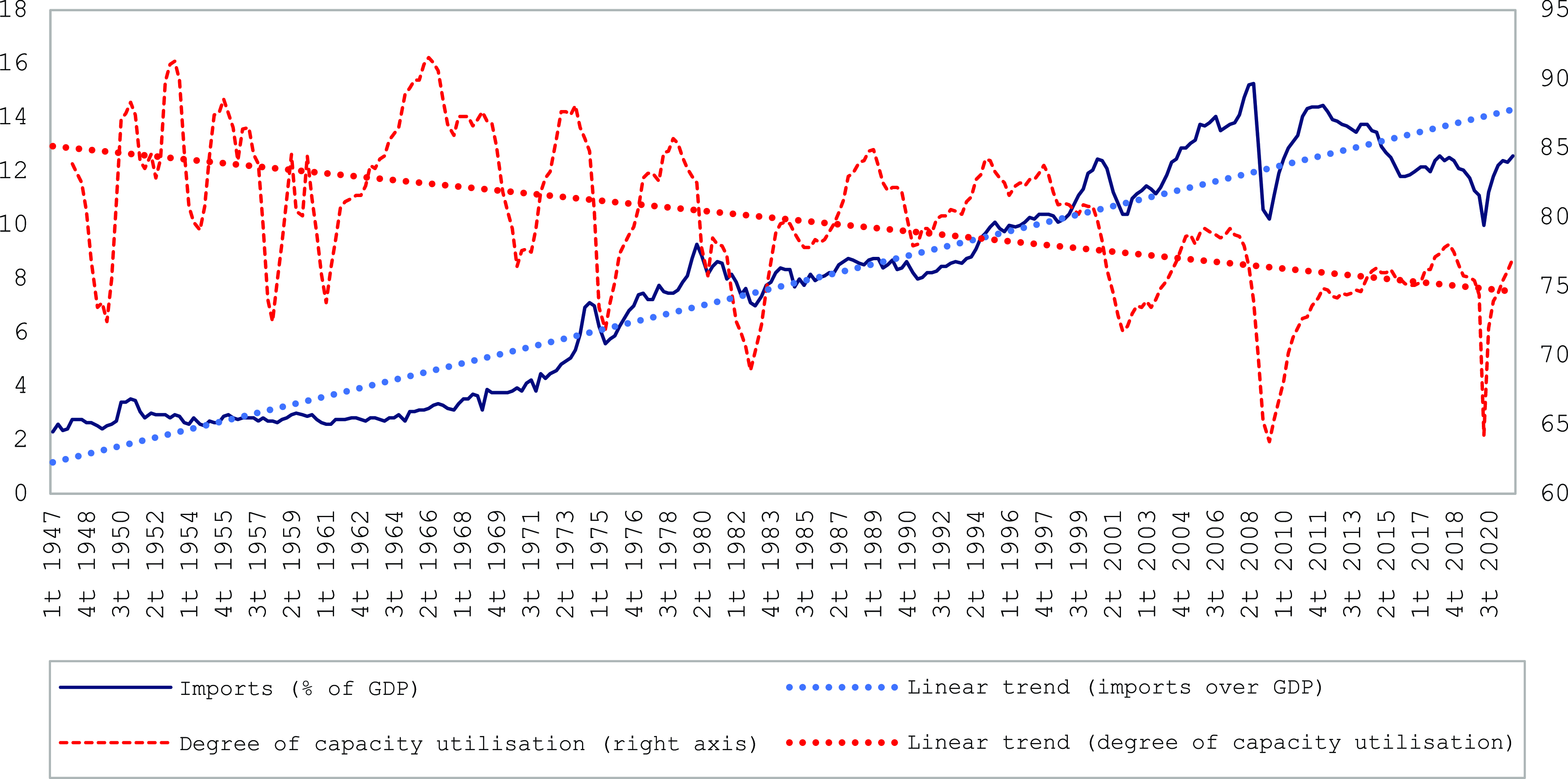
Graph 3. Weight of imports over GDP and degree of productive capacity utilisation in the United States (%), 1947–2020.
In the next section, we use quarterly US data to analyse the causal relationship between the propensity to import $({\rm{m}}$
), the degree of productive capacity utilisation (
$({\rm{m}}$
), the degree of productive capacity utilisation ( ${\rm{u}}$
), and capital productivity (
${\rm{u}}$
), and capital productivity ( ${\rm{\pi k}}$
) between 1947 and 2019.
${\rm{\pi k}}$
) between 1947 and 2019.
Empirical analysis
We study hysteresis and contemporaneous relationships between the propensity to import $({\rm{m}}$
), the degree of productive capacity utilisation (
$({\rm{m}}$
), the degree of productive capacity utilisation ( ${\rm{u}}$
), and capital productivity (
${\rm{u}}$
), and capital productivity ( ${\rm{\pi k}}$
) between 1947 and 2019. We use time-varying impulse-response analysis and directed acyclic graphs (DAG) for this aim.
${\rm{\pi k}}$
) between 1947 and 2019. We use time-varying impulse-response analysis and directed acyclic graphs (DAG) for this aim.
Time-varying impulse-response functions
The Lumsdaine-Papell and Bai-Perron’s unit root tests indicate that the variables under study have multiple and different structural breaks. Thus, instead of dividing the entire test into sub-periods, we use a time-varying parameter structural vector autoregressive (TVP-SVAR) model on the total sample. Unlike standard SVAR models, which impose the constraint that the coefficients are constant through time, the TVP-SVAR allows continuous smooth changes in the coefficients.
Following Sims (Reference Sims1980) and Sims et al (Reference Sims, Stock and Watson1990), who claim that a VAR in levels correctly estimates the dynamics of a system,Footnote 2 we estimate a TVP-SVAR in levels, which is usual in the VAR literature (Elbourne Reference Elbourne2008; Farzanegan and Markwardt Reference Farzanegan and Markwardt2009; Tang et al Reference Tang, Wu and Zhang2010; Iwayemi and Fowowe Reference Iwayemi and Fowowe2011; Alom et al Reference Alom, Ward and Hu2013; Kohler and Stockhammer Reference Kohler and Stockhammer2020, among others). The fact that some of the variables are I(1) is not a problem since the slope coefficients of the I(1) variables could be rewritten as differenced variable coefficients (Stockhammer et al Reference Stockhammer, Calvert Jump, Kohler and Cavallero2019). Furthermore, using the variables in a VAR representation in levels ‘avoids the controversial question of which cointegration constraints impose in the estimate’ (Kilian and Lütkepohl Reference Kilian and Lütkepohl2017).
To order the variables in the SVAR model, we have used the DAG method, a data-driven method of ordering the data in a VAR model, thereby avoiding theoretical assumptions. To this aim, we use the PC algorithm of Spirtes et al (Reference Spirtes, Glymour and Scheines2000). Because simultaneity or instantaneous causality may appear due to omitted causal variables, Spirtes et al (Reference Spirtes, Glymour and Scheines2000) have developed methods for inferring the existence of omitted (latent) variables and working out their causal consequences (Hoover Reference Hoover2005: 74). The empirical literature considers the use of the PC algorithm as a valid tool to assign causal flows among variables based on observational data: Kalisch and Buhlmann (Reference Kalisch and Buhlmann2007) show that the PC algorithm using statistical tests is computationally feasible and consistent even for very high-dimensional sparse DAGs; while Uhler et al (Reference Uhler, Raskutti, Bülmann and Yu2013) show that additionally assuming a condition called strong faithfulness, the PC algorithm even yields uniform consistency. Finally, Demiralp and Hooverà (Reference Demiralp and Hooverà2003) study the PC algorithm with Monte Carlo simulations and show that the DAG is a valid statistical procedure to identify the contemporaneous causal order of a structural vector autoregression.
A directed acyclic graph analysis is a directed graph with no loop. It is composed of points representing variables and directed edges connecting these points. The DAG analysis uses graphs to represent the contemporaneous causal relationships between variables. In a directed acyclic graph, the direct edge between two points represents the contemporaneous causal relationship between two variables. The possibilities between two variables, A and B, are the following:
-
A → B: represents that A contemporaneously causes B;
-
A ← B: states that B contemporaneously causes A;
-
A↔B: indicates that there is bidirectional contemporaneous causality between A and B;
-
A–B: represents that there is a contemporaneous causality with uncertain direction between A and B;
-
A B indicates that there is not any contemporaneous causality between A and B.
We use the PC algorithm by Spirtes et al (Reference Spirtes, Glymour and Scheines2000) to analyse the contemporaneous causal relationships between the variables. We built a full non-directed graph with three variables, each connected to the other two. Hereafter, we remove and direct the edges of the full non-directed graph. In the phase of removal, we first analyse the unconditional correlation coefficient and eliminate the edge connecting both variables when the correlation coefficient between them is 0. Once we have finished the correlation analysis, we analyse the first-order partial correlation coefficient (the correlation coefficient between two variables conditional on the third variable) on the remaining edges. The edge that connects both variables is removed when the first-order correlation coefficient between the two variables is 0. Likewise, after completing the first-order partial correlation coefficient analysis, the second-order partial correlation coefficient is analysed on the remaining edges, and subsequently, the third-order, …, until the N-2-order partial correlation coefficient. In our case, as N = 3, we only analyse the first-order partial correlation coefficient. To test whether the partial correlation coefficients are significantly different from 0, we use Fisher’s z-statistic.
Once we have ordered the variables, we estimate the TVP-SVAR model with two lags (based on the Bayesian information criteria of Schwarz (Reference Schwarz1978) and the Hannan-Quinn information criterion of Hannan and Quinn (Reference Hannan and Quinn1979)). We aim to capture the time-varying impacts that structural shocks on ${\rm{m\;}}$
(
${\rm{m\;}}$
( ${\rm{u}}$
) have on
${\rm{u}}$
) have on ${\rm{u}}$
(
${\rm{u}}$
( ${\rm{\pi k}}$
) without dividing our full sample into subsamples. Indeed, compared to the constant parameters SVAR model, the TVP-SVAR models allow the detection of the changes in the responses’ behaviour over time of the system to the identified structural shocks while conserving the full sample information specificity (Zhong et al Reference Zhong, Zhang and Ren2023, 106708). The uncorrelatedness of the shocks allows us to identify impulse-response functions and rules out the presence of any omitted variables that enter multiple equations (Ghanem and Smith Reference Ghanem and Smith2022).
${\rm{\pi k}}$
) without dividing our full sample into subsamples. Indeed, compared to the constant parameters SVAR model, the TVP-SVAR models allow the detection of the changes in the responses’ behaviour over time of the system to the identified structural shocks while conserving the full sample information specificity (Zhong et al Reference Zhong, Zhang and Ren2023, 106708). The uncorrelatedness of the shocks allows us to identify impulse-response functions and rules out the presence of any omitted variables that enter multiple equations (Ghanem and Smith Reference Ghanem and Smith2022).
The DAG analysis, whose results are presented in Figure 1, suggests ordering the variables in the TVP-SVAR as follows: ${\rm{m}}$
,
${\rm{m}}$
, ${\rm{u}}$
,
${\rm{u}}$
, ${\rm{\pi k}}$
. Once the restrictions are imposed, and the model is estimated, we compute time-varying impulse-response functions to assess the impact of an exogenous shock in
${\rm{\pi k}}$
. Once the restrictions are imposed, and the model is estimated, we compute time-varying impulse-response functions to assess the impact of an exogenous shock in ${\rm{m}}$
,
${\rm{m}}$
, ${\rm{u}}$
, and
${\rm{u}}$
, and ${\rm{\pi k}}$
. We compute standard errors using the Monte Carlo method (1,000 repetitions) and report the IRFs with one-standard error band, namely a 68% confidence interval.Footnote
3
Figure 1 also shows the results of the impulse-response functions based on the TVP-SVAR model’s specification with the three variables in levels. It allows us to analyse the relationship between the variables under study on the entire sample interval. On the left-hand side of Figure 1, we can see the impulse-response paths of
${\rm{\pi k}}$
. We compute standard errors using the Monte Carlo method (1,000 repetitions) and report the IRFs with one-standard error band, namely a 68% confidence interval.Footnote
3
Figure 1 also shows the results of the impulse-response functions based on the TVP-SVAR model’s specification with the three variables in levels. It allows us to analyse the relationship between the variables under study on the entire sample interval. On the left-hand side of Figure 1, we can see the impulse-response paths of ${\rm{u}}\;$
to a positive shock in
${\rm{u}}\;$
to a positive shock in ${\rm{m}}$
. We found that an exogenous positive shock on the import share significantly negatively affects the degree of capacity utilisation. In contrast, a shock on
${\rm{m}}$
. We found that an exogenous positive shock on the import share significantly negatively affects the degree of capacity utilisation. In contrast, a shock on ${\rm{u}}$
does not significantly affect
${\rm{u}}$
does not significantly affect ${\rm{m}}$
. We also observe that a positive shock on
${\rm{m}}$
. We also observe that a positive shock on ${\rm{u}}$
has a positive and significant effect on
${\rm{u}}$
has a positive and significant effect on ${\rm{\pi k}}$
. In contrast, an exogenous positive shock on
${\rm{\pi k}}$
. In contrast, an exogenous positive shock on ${\rm{\pi k}}$
does not significantly affect
${\rm{\pi k}}$
does not significantly affect ${\rm{u}}$
.
${\rm{u}}$
.

Figure 1. Responses of m, u, and πk to time-varying shocks in m, u, and πk. Note: The vertical axis shows the value of the parameters, while the horizontal axis shows the time horizon (quarters). The shaded area is the 68% error band.
Contemporaneous causality
Since there are not only hysteresis relationships between macroeconomic variables, we also explore the existence of contemporaneous causal relationships. The loss of market share can contemporaneously affect aggregate demand, consequently affecting capacity utilisation and thus, capital productivity. The VAR approach does not allow the study of the contemporaneous relationships between variables, which remain hidden in the model’s error term and cannot be estimated. Therefore, we use the DAG analysis to study contemporaneous relationships between ${{\rm{m}}_{\rm{t}}}$
,
${{\rm{m}}_{\rm{t}}}$
, ${{\rm{u}}_{\rm{t}}}$
, and
${{\rm{u}}_{\rm{t}}}$
, and ${\rm{\pi }}{{\rm{k}}_{\rm{t}}}$
. Following our hypothesis, we study the contemporaneous causal relationship between positive changes in m (
${\rm{\pi }}{{\rm{k}}_{\rm{t}}}$
. Following our hypothesis, we study the contemporaneous causal relationship between positive changes in m ( ${\rm{m}}_{\rm{t}}^ + $
), negative changes in u (
${\rm{m}}_{\rm{t}}^ + $
), negative changes in u ( ${\rm{u}}_{\rm{t}}^ - $
), and negative changes in
${\rm{u}}_{\rm{t}}^ - $
), and negative changes in ${\rm{\pi k}}$
(
${\rm{\pi k}}$
( ${\rm{\pi k}}_{\rm{t}}^ - $
). To build
${\rm{\pi k}}_{\rm{t}}^ - $
). To build ${\rm{m}}_{\rm{t}}^ + $
,
${\rm{m}}_{\rm{t}}^ + $
, ${\rm{u}}_{\rm{t}}^ - $
, and
${\rm{u}}_{\rm{t}}^ - $
, and ${\rm{\pi k}}_{\rm{t}}^ - $
, we use the partial sum decompositions of Hatemi-J (Reference Hatemi-J2012, Reference Hatemi-J2014) and Hatemi-El-Khatib (Reference Hatemi and El-Khatib2016). This enables us to study the causal relationship between positive (negative) changes in one variable and positive (negative) changes in another variable or any other combination (Hatemi-J et al Reference Hatemi-J, Al Shayeb and Roca2017). Thus, this method allows us to study whether a negative change in the utilisation degree of productive capacity is contemporaneously caused by a positive change in the propensity to import. We can also study whether a decrease in the degree of capacity utilisation contemporaneously causes a negative change in capital productivity.
${\rm{\pi k}}_{\rm{t}}^ - $
, we use the partial sum decompositions of Hatemi-J (Reference Hatemi-J2012, Reference Hatemi-J2014) and Hatemi-El-Khatib (Reference Hatemi and El-Khatib2016). This enables us to study the causal relationship between positive (negative) changes in one variable and positive (negative) changes in another variable or any other combination (Hatemi-J et al Reference Hatemi-J, Al Shayeb and Roca2017). Thus, this method allows us to study whether a negative change in the utilisation degree of productive capacity is contemporaneously caused by a positive change in the propensity to import. We can also study whether a decrease in the degree of capacity utilisation contemporaneously causes a negative change in capital productivity.
Let us assume that ${\rm{\pi }}{{\rm{k}}_{\rm{t}}}$
,
${\rm{\pi }}{{\rm{k}}_{\rm{t}}}$
, ${{\rm{u}}_{\rm{t}}}$
, and
${{\rm{u}}_{\rm{t}}}$
, and ${{\rm{m}}_{\rm{t}}}$
have the same data generation process:
${{\rm{m}}_{\rm{t}}}$
have the same data generation process: ${\rm{\pi }}{{\rm{k}}_{\rm{t}}} \equiv {\rm{\pi }}{{\rm{k}}_{{\rm{t}} - 1}} + {{\rm{e}}_{1{\rm{t}}}} = {\rm{\pi }}{{\rm{k}}_0} + \mathop \sum \limits_{{\rm{i}} = 1}^{\rm{T}} {{\rm{e}}_{1{\rm{i}}}}$
,
${\rm{\pi }}{{\rm{k}}_{\rm{t}}} \equiv {\rm{\pi }}{{\rm{k}}_{{\rm{t}} - 1}} + {{\rm{e}}_{1{\rm{t}}}} = {\rm{\pi }}{{\rm{k}}_0} + \mathop \sum \limits_{{\rm{i}} = 1}^{\rm{T}} {{\rm{e}}_{1{\rm{i}}}}$
, ${{\rm{u}}_{\rm{t}}} \equiv {{\rm{u}}_{{\rm{t}} - 1}} + {{\rm{e}}_{2{\rm{t}}}} = {{\rm{u}}_0} + \mathop \sum \limits_{{\rm{i}} = 1}^{\rm{T}} {{\rm{e}}_{2{\rm{i}}}}$
, and
${{\rm{u}}_{\rm{t}}} \equiv {{\rm{u}}_{{\rm{t}} - 1}} + {{\rm{e}}_{2{\rm{t}}}} = {{\rm{u}}_0} + \mathop \sum \limits_{{\rm{i}} = 1}^{\rm{T}} {{\rm{e}}_{2{\rm{i}}}}$
, and ${{\rm{m}}_{\rm{t}}} \equiv {{\rm{m}}_{{\rm{t}} - 1}} + {{\rm{e}}_{3{\rm{t}}}} = {{\rm{m}}_0} + \mathop \sum \limits_{{\rm{i}} = 1}^{\rm{T}} {{\rm{e}}_{3{\rm{i}}}}$
, being
${{\rm{m}}_{\rm{t}}} \equiv {{\rm{m}}_{{\rm{t}} - 1}} + {{\rm{e}}_{3{\rm{t}}}} = {{\rm{m}}_0} + \mathop \sum \limits_{{\rm{i}} = 1}^{\rm{T}} {{\rm{e}}_{3{\rm{i}}}}$
, being ${\rm{\pi }}{{\rm{k}}_0}$
,
${\rm{\pi }}{{\rm{k}}_0}$
, ${{\rm{u}}_0}$
, and
${{\rm{u}}_0}$
, and ${{\rm{m}}_0}$
the initial values of
${{\rm{m}}_0}$
the initial values of ${\rm{\pi }}{{\rm{k}}_{\rm{t}}}$
,
${\rm{\pi }}{{\rm{k}}_{\rm{t}}}$
, ${{\rm{u}}_{\rm{t}}}$
, and
${{\rm{u}}_{\rm{t}}}$
, and ${{\rm{m}}_{\rm{t}}}$
respectively, while
${{\rm{m}}_{\rm{t}}}$
respectively, while ${{\rm{e}}_{1{\rm{i}}}}$
,
${{\rm{e}}_{1{\rm{i}}}}$
, ${{\rm{e}}_{2{\rm{i}}}},{\rm{\;}}$
and
${{\rm{e}}_{2{\rm{i}}}},{\rm{\;}}$
and ${{\rm{e}}_{3{\rm{i}}}}$
are i.i.d with
${{\rm{e}}_{3{\rm{i}}}}$
are i.i.d with ${\rm{\sigma }}_{{{\rm{e}}_1}}^2$
,
${\rm{\sigma }}_{{{\rm{e}}_1}}^2$
, ${\rm{\sigma }}_{{{\rm{e}}_2}}^2$
y
${\rm{\sigma }}_{{{\rm{e}}_2}}^2$
y ${\rm{\sigma }}_{{{\rm{e}}_3}}^2$
variance, respectively. Hatemi-J (Reference Hatemi-J2012, Reference Hatemi-J2014) defines positive shocks as
${\rm{\sigma }}_{{{\rm{e}}_3}}^2$
variance, respectively. Hatemi-J (Reference Hatemi-J2012, Reference Hatemi-J2014) defines positive shocks as ${\rm{e}}_{1{\rm{t}}}^ + = {\rm{max}}\left( {{{\rm{e}}_{1{\rm{t}}}},0} \right)$
,
${\rm{e}}_{1{\rm{t}}}^ + = {\rm{max}}\left( {{{\rm{e}}_{1{\rm{t}}}},0} \right)$
, ${\rm{e}}_{2{\rm{t}}}^ + = {\rm{max}}\left( {{{\rm{e}}_{2{\rm{t}}}},0} \right)$
and
${\rm{e}}_{2{\rm{t}}}^ + = {\rm{max}}\left( {{{\rm{e}}_{2{\rm{t}}}},0} \right)$
and ${\rm{e}}_{3{\rm{t}}}^ + = {\rm{max}}\left( {{{\rm{e}}_{3{\rm{t}}}},0} \right);$
while he represents negative shocks as
${\rm{e}}_{3{\rm{t}}}^ + = {\rm{max}}\left( {{{\rm{e}}_{3{\rm{t}}}},0} \right);$
while he represents negative shocks as ${\rm{e}}_{1{\rm{t}}}^ - = {\rm{min}}\left( {{{\rm{e}}_{1{\rm{t}}}},0} \right),{\rm{\;e}}_{2{\rm{t}}}^ - = {\rm{min}}\left( {{{\rm{e}}_{2{\rm{t}}}},0} \right)$
and
${\rm{e}}_{1{\rm{t}}}^ - = {\rm{min}}\left( {{{\rm{e}}_{1{\rm{t}}}},0} \right),{\rm{\;e}}_{2{\rm{t}}}^ - = {\rm{min}}\left( {{{\rm{e}}_{2{\rm{t}}}},0} \right)$
and ${\rm{e}}_{3{\rm{t}}}^ - = {\rm{min}}\left( {{{\rm{e}}_{3{\rm{t}}}},0} \right)$
. Therefore,
${\rm{e}}_{3{\rm{t}}}^ - = {\rm{min}}\left( {{{\rm{e}}_{3{\rm{t}}}},0} \right)$
. Therefore, ${{\rm{e}}_{1{\rm{t}}}} = {\rm{e}}_{1{\rm{t}}}^ + + {\rm{e}}_{1{\rm{t}}}^ - $
,
${{\rm{e}}_{1{\rm{t}}}} = {\rm{e}}_{1{\rm{t}}}^ + + {\rm{e}}_{1{\rm{t}}}^ - $
, ${{\rm{e}}_{2{\rm{t}}}} = {\rm{e}}_{2{\rm{t}}}^ + + {\rm{e}}_{2{\rm{t}}}^ - $
, and
${{\rm{e}}_{2{\rm{t}}}} = {\rm{e}}_{2{\rm{t}}}^ + + {\rm{e}}_{2{\rm{t}}}^ - $
, and ${{\rm{e}}_{3{\rm{t}}}} = {\rm{e}}_{3{\rm{t}}}^ + + {\rm{e}}_{3{\rm{t}}}^ - $
; while
${{\rm{e}}_{3{\rm{t}}}} = {\rm{e}}_{3{\rm{t}}}^ + + {\rm{e}}_{3{\rm{t}}}^ - $
; while ${\rm{\pi }}{{\rm{k}}_{\rm{t}}} = {\rm{\pi }}{{\rm{k}}_0} + \mathop \sum \limits_{{\rm{i}} = 1}^{\rm{t}} {\rm{e}}_{1{\rm{t}}}^ + + \mathop \sum \limits_{{\rm{i}} = 1}^{\rm{t}} {\rm{e}}_{1{\rm{t}}}^ - $
,
${\rm{\pi }}{{\rm{k}}_{\rm{t}}} = {\rm{\pi }}{{\rm{k}}_0} + \mathop \sum \limits_{{\rm{i}} = 1}^{\rm{t}} {\rm{e}}_{1{\rm{t}}}^ + + \mathop \sum \limits_{{\rm{i}} = 1}^{\rm{t}} {\rm{e}}_{1{\rm{t}}}^ - $
, ${{\rm{u}}_{\rm{t}}} = {{\rm{u}}_0} + \mathop \sum \limits_{{\rm{i}} = 1}^{\rm{t}} {\rm{e}}_{2{\rm{t}}}^ + + \mathop \sum \limits_{{\rm{i}} = 1}^{\rm{t}} {\rm{e}}_{2{\rm{t}}}^ - $
, and
${{\rm{u}}_{\rm{t}}} = {{\rm{u}}_0} + \mathop \sum \limits_{{\rm{i}} = 1}^{\rm{t}} {\rm{e}}_{2{\rm{t}}}^ + + \mathop \sum \limits_{{\rm{i}} = 1}^{\rm{t}} {\rm{e}}_{2{\rm{t}}}^ - $
, and ${{\rm{m}}_{\rm{t}}} = {{\rm{m}}_0} + \mathop \sum \limits_{{\rm{i}} = 1}^{\rm{t}} {\rm{e}}_{3{\rm{t}}}^ + + \mathop \sum \limits_{{\rm{i}} = 1}^{\rm{t}} {\rm{e}}_{3{\rm{t}}}^ - $
. In this way, and following Granger and Yoon (Reference Granger and Yoon2002), Hatemi-J (Reference Hatemi-J2012) defines accumulative positive and negative shocks as:
${{\rm{m}}_{\rm{t}}} = {{\rm{m}}_0} + \mathop \sum \limits_{{\rm{i}} = 1}^{\rm{t}} {\rm{e}}_{3{\rm{t}}}^ + + \mathop \sum \limits_{{\rm{i}} = 1}^{\rm{t}} {\rm{e}}_{3{\rm{t}}}^ - $
. In this way, and following Granger and Yoon (Reference Granger and Yoon2002), Hatemi-J (Reference Hatemi-J2012) defines accumulative positive and negative shocks as: ${\rm{\pi k}}_{\rm{t}}^ + = \mathop \sum \limits_{{\rm{i}} = 1}^{\rm{t}} {\rm{e}}_{1{\rm{t}}}^ + $
;
${\rm{\pi k}}_{\rm{t}}^ + = \mathop \sum \limits_{{\rm{i}} = 1}^{\rm{t}} {\rm{e}}_{1{\rm{t}}}^ + $
; ${\rm{\pi k}}_{\rm{t}}^ - = \mathop \sum \limits_{{\rm{i}} = 1}^{\rm{t}} {\rm{e}}_{1{\rm{i}}}^ - $
;
${\rm{\pi k}}_{\rm{t}}^ - = \mathop \sum \limits_{{\rm{i}} = 1}^{\rm{t}} {\rm{e}}_{1{\rm{i}}}^ - $
; ${\rm{u}}_{\rm{t}}^ + = \mathop \sum \limits_{{\rm{i}} = 1}^{\rm{t}} {\rm{e}}_{2{\rm{t}}}^ + $
;
${\rm{u}}_{\rm{t}}^ + = \mathop \sum \limits_{{\rm{i}} = 1}^{\rm{t}} {\rm{e}}_{2{\rm{t}}}^ + $
; ${\rm{u}}_{\rm{t}}^ - = \mathop \sum \limits_{{\rm{i}} = 1}^{\rm{t}} {\rm{e}}_{2{\rm{i}}}^ - $
;
${\rm{u}}_{\rm{t}}^ - = \mathop \sum \limits_{{\rm{i}} = 1}^{\rm{t}} {\rm{e}}_{2{\rm{i}}}^ - $
; ${\rm{m}}_{\rm{t}}^ + = \mathop \sum \limits_{{\rm{i}} = 1}^{\rm{t}} {\rm{e}}_{3{\rm{t}}}^ + $
; and
${\rm{m}}_{\rm{t}}^ + = \mathop \sum \limits_{{\rm{i}} = 1}^{\rm{t}} {\rm{e}}_{3{\rm{t}}}^ + $
; and ${\rm{m}}_{\rm{t}}^ - = \mathop \sum \limits_{{\rm{i}} = 1}^{\rm{t}} {\rm{e}}_{3{\rm{i}}}^ - $
.
${\rm{m}}_{\rm{t}}^ - = \mathop \sum \limits_{{\rm{i}} = 1}^{\rm{t}} {\rm{e}}_{3{\rm{i}}}^ - $
.
Once we obtain ${\rm{m}}_{\rm{t}}^ + $
,
${\rm{m}}_{\rm{t}}^ + $
, ${\rm{u}}_{\rm{t}}^ - $
, and
${\rm{u}}_{\rm{t}}^ - $
, and ${\rm{\pi k}}_{\rm{t}}^ - $
, the next step is building a non-directed full graph of
${\rm{\pi k}}_{\rm{t}}^ - $
, the next step is building a non-directed full graph of ${\rm{m}}_{\rm{t}}^ + $
,
${\rm{m}}_{\rm{t}}^ + $
, ${\rm{u}}_{\rm{t}}^ - $
and
${\rm{u}}_{\rm{t}}^ - $
and ${\rm{\pi k}}_{\rm{t}}^ - $
. Next, we analyse the matrix of the remaining coefficients by the PC algorithm of the Tetrad software to obtain the contemporaneous causal relationships between
${\rm{\pi k}}_{\rm{t}}^ - $
. Next, we analyse the matrix of the remaining coefficients by the PC algorithm of the Tetrad software to obtain the contemporaneous causal relationships between ${\rm{m}}_{\rm{t}}^ + $
,
${\rm{m}}_{\rm{t}}^ + $
, ${\rm{u}}_{\rm{t}}^ - $
, and
${\rm{u}}_{\rm{t}}^ - $
, and ${\rm{\pi k}}_{\rm{t}}^ - $
(Figure 2):
${\rm{\pi k}}_{\rm{t}}^ - $
(Figure 2):

Figure 2. DAG analysis between m+, u-, and πk-. Note: Directed acyclic graphs between ${\rm{m}}_{\rm{t}}^ + $
,
${\rm{m}}_{\rm{t}}^ + $
, ${\rm{u}}_{\rm{t}}^ - $
, and
${\rm{u}}_{\rm{t}}^ - $
, and ${\rm{\pi k}}_{\rm{t}}^ - $
. The asterisks *** denote statistical significance at the 1%.
${\rm{\pi k}}_{\rm{t}}^ - $
. The asterisks *** denote statistical significance at the 1%.
As shown in Figure 2, ${\rm{u}}_{\rm{t}}^ - $
is a contemporaneous cause of
${\rm{u}}_{\rm{t}}^ - $
is a contemporaneous cause of ${\rm{\pi k}}_{\rm{t}}^ - $
, while
${\rm{\pi k}}_{\rm{t}}^ - $
, while ${\rm{m}}_{\rm{t}}^ + $
contemporaneously causes
${\rm{m}}_{\rm{t}}^ + $
contemporaneously causes ${\rm{u}}_{\rm{t}}^ - $
. This indicates that the loss of market shares by the US resident productive sector contemporaneously reduces the utilisation degree of productive capacity of the United States, which in turn, contemporaneously causes a decrease in capital productivity.
${\rm{u}}_{\rm{t}}^ - $
. This indicates that the loss of market shares by the US resident productive sector contemporaneously reduces the utilisation degree of productive capacity of the United States, which in turn, contemporaneously causes a decrease in capital productivity.
Discussion
We have proposed an overall but consistent possible explanation of the loss of US industrial economic dynamism in the framework of increasing globalisation. Departing from the preposition that the adjustment of capacity to demand is slow in the US (Haluska et al Reference Haluska, Summa and Serrano2023), we have hypothesised a causal relation between market loss (proxied by an increasing propensity to import) and a decrease of both productive capacity utilisation and capital productivity. What does this mean? The answer might seem only intuitive, but in our opinion, it is clear.
The 1970s crisis sponsored the abandonment of industrial policy and the liberalisation and globalisation of markets instead of triggering a resurgence of industrial-based technology policies. Thus, a profound change in economic policy priorities took place. Due to the shock in production costs caused by the energy crisis, the productive system was abandoned to its fate and had to face an unstoppable growth of imports. These imports helped to contain inflation, the main goal of the new neoliberal economic policy of the moment.
This economic policy prioritised monetary policy and abandoned previous full employment strategies of Keynesian inspiration (Armstrong et al Reference Armstrong, Glyn and Harrison1991b). As a result, significant and strategic parts of US production were squandered and replaced by foreign production, often due to relocations promoted by US multinational companies. The central core of the US industrial productive system, which survived the deep crisis of the 1970s, had to contend with a new neoliberal economic policy paradigm, facing more international competition. This change hurt the rate of profit of non-financial resident firms through the decrease in capacity utilisation. In turn, increasing foreign competition led US resident firms to the renewal of the productive equipment. This demanded more production and market share to increase production per unit of capital invested. However, instead, what happened is that foreign productions, including those of US transnational capital, gained more and more domestic market share. This caused a further fall in the utilisation degree of productive equipment and a continued decrease in capital productivity and levels of profitability of productive capital.
In order to counteract the decreasing trend in the rate of profit, the resident productive sector took advantage of the new economic paradigm to contain wages (as argued by Basu et al (Reference Basu, Huato, Jauregui and Wasner2022) and empirically demonstrated by Manera et al (Reference Manera, Navines, Perez-Montiel and Franconetti2022) and Tippet et al (Reference Tippet, Onaran and Wildauer2022)). Simultaneously, the tax burden on capital income and corporate social contributions was reduced, with the consequent reduction of the Welfare State and increased social polarisation. The described process involves an increase in income inequality, resulting from the purpose of resident corporate capital to maintain its profits. In this sense, other researchers’ provided data align with our conclusion (Hacker and Pierson Reference Hacker and Pierson2010; Saez and Zucman Reference Saez and Zucman2022). In fact, between 1980 and 2018, the US witnessed a slowdown in growth parallel to a greater concentration of incomes and wealth (Espinosa-Gracia and Sánchez-Chóliz Reference Espinosa-Gracia and Sánchez-Chóliz2023): the incomes of the top 0.1% of income earners have grown by 320% since 1980. At the same time, the top 0.01% increased its income by 430%, while the incomes of the 0.001% have grown by 600%. Simultaneously, the working class has yet to experience income increases in real terms (Austin Reference Austin2013).
Conclusions
Capitalism is failing to develop productive forces globally and take humanity forward to a world of prosperity and the end of toil, poverty, and inequality (Roberts Reference Roberts2022, 18). A key measure of the productive forces’ development is capital productivity. In this paper, we argue that the decrease in capital productivity (proxied by the output/capital ratio) is the main cause of the decline in the profit rate in the United States.
So, what has been the main cause of the decrease of the output/capital ratio in the US? Why has the US capitalism, with its technological innovation capabilities, been unable to prevent its capital productivity from dropping? We argue that the 1970s entailed the abandonment of industrial policy and the liberalisation and globalisation of markets, which left the US productive sector at the mercy of the unstoppable growth of imports. These imports, which helped contain inflation, hoarded the US domestic market, which negatively affected the degree of productive capacity utilisation and the profit rate of the productive resident US firms. Increasing foreign competition demanded the renewal of productive equipment, and this new equipment demanded greater production volumes and more market shares to increase production per unit of invested capital. However, the domestic market share of US-resident companies declined in favour of non-resident firms. This explains the relentless fall in the utilisation degree of productive equipment and capital productivity since the 1980s.
Given the real wage, secular falls in capital productivity imply the reduction of the ex-post rate of profit. The decreasing profit rate’s most noticeable consequences are the firm sector’s political reaction to contain wages and the growing transfer of capital from the productive sector to the financial sector. In sum, from 1980 onwards, the change in the regulatory system of the US economy, which switched from Keynesian to neoliberal regulation, led to an increasing globalisation of the US economy. This has led to increasing tertiarisation, financialisation, property speculation, and inequality in the United States.
Acknowledgements
We are grateful to two anonymous reviewers and the editor for valuable comments and suggestions that helped to considerably improve the paper. Usual disclaimers apply.
Funding statement
This work has been carried out thanks to the financial support of the research projects PGC 2018-093896-B-I00 and PID2022-137648OB-C21, funded by Ministerio de Ciencia e Innovación (Madrid), MCIN/AEI/ 10.13039/501100011033 and by the European Regional Development Fund, ‘ERDF A way of making Europe’.
Competing interests
There are no potential or perceived conflicts of interest.
José A. Pérez-Montiel: Associate professor of economics at the University of the Balearic Islands (Spain) and research director at the Angelo King Institute for Economic and Business Studies (Philippines). Carles Manera: Full professor of economics at the University of the Balearic Islands (Spain) and advisor of the Governor of the Bank of Spain. Ferran Navinés: Associate professor of economics (retired) at the university of Girona (Spain) and senior economist (retired) at the Government of the Balearic Islands. Javier Franconetti: Associate professor at the Higher Education Center Felipe Moreno (Universidad Nebrija, Spain) and professor at the University of the Balearic Islands (Spain).


 Open access