

1. Introduction
Suppose you have 200 dollars, and want to use it to do the most good you can. Some ways you could use it are nearly certain to result in more total good: for example, you could donate it to your local food bank, which will almost certainly result in fewer people going hungry. Other ways you could use it may result in more good, or may result in almost no improvement at all: for example, if your area has a 30% chance of a major earthquake in the next 50 years, you could donate it to an organization that distributes earthquake preparedness kits; if an earthquake happens, donating to this organization will do substantially more good than donating to the food bank will, but if not, doing so will do substantially less good. Still other ways to use the money may or may not result in a change to the overall good, but you may not be able to put a precise probability on this: for example, you could donate it to a highly experimental start-up, which may succeed in reducing poverty, but may fail, where it's difficult to determine the probability of success.
The same question reappears at the level of national and international aid. We must choose between funding various types of causes, each of which may do various amounts of good with various probabilities; in addition, we may not always be able to determine the probabilities precisely. Even when we make choices among programs that address the same problem, we may not know which of two programs or organizations is apt to be more successful.
This article concerns how to make choices whose sole purpose is to do the most good, when you cannot be certain of the consequences of the alternatives. When you are uncertain of the consequences of various alternatives, you cannot choose precisely to bring about the most good, but instead must choose to bring about the best gamble among possibilities with varying levels of goodness. It is typically assumed that to choose the best gamble is to maximize expected utility; but recent work has challenged the idea that this is the correct framework for rational and moral decision-making. In particular, some have argued contra this framework that we can be risk-avoidant or risk-inclined and we can be ambiguity-averse or ambiguity-seeking. The goal of this article is to determine how these attitudes make a difference to which causes we should give to.
We will focus on two questions. First, when we give money purely with the intent of bringing about the best gamble, to what extent should we diversify among the programs that we give to? Second, when we're choosing between giving to a program that has a known, high probability of doing good (for example, a health amelioration program) and another program that has a very small or perhaps unknown probability of doing much more good (for example, a program that makes the already-small and perhaps unknown probability of nuclear annihilation even smaller), which should we choose? We will see how our attitudes towards risk and ambiguity affect the answers to each of these questions.
2. Expected utility and extensions
Readers who are already familiar with expected utility, risk-weighted expected utility, and α-maximin can skip to section 3.
2.1 Expected utility
The most well-known formal theories of decision-making under uncertainty tell us how to evaluate acts, where an act is an assignment of consequences to states of the world.Footnote 1 For example, the act of going to the beach assigns consequence <I have an unpleasant time> to the state in which the weather is cold, <I have an okay time> to the state in which it is warm, and <I have a great time> to the state in which it is hot. We can represent this act as {COLD, I have an unpleasant time; WARM, I have an okay time; HOT, I have a great time}. Each consequence has a utility value; we can thus write these acts as assignments of utility values to states of the world, for example {COLD, 2; WARM, 3; HOT, 6}.Footnote 2
In the classical theory, we can additionally assign sharp probabilities to states of the world; for example, we might assign probability 0.2 to the weather being cold, 0.4 to it being warm, and 0.4 to it being hot, so that we can represent the act as {2, 0.2; 3, 0.4; 6, 0.4}. It is rational to choose or prefer acts with the highest expected utility, where expected utility is a weighted average of the utilities of each consequence, each utility value weighted by the probability of the state in which it obtains.Footnote 3 Graphically, if the height of each bar represents utility, and its width probability, expected utility is the area under the curve in Figure 1.Footnote 4 In this case, the value of the gamble ‘go to the beach’ will be (0.2)(2) + (0.4)(3) + (0.4)(6) = 4.

Figure 1. Expected utility.
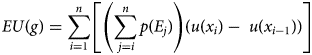
Formally, let ${\rm \succeq }$ represent some individual's preference relation, with ≻ and ≈ defined in the usual way. Then let g = {E1, x1; …; En, xn} be a gamble that yields outcome xi in event Ei. Let p(Ei) be the subjective probability of Ei, and let u(xi) be the utility of xi. The expected utility of g is:

One way to think about expected utility conceptually is this. An act has possible consequences, and the amount each consequence matters in determining the total value of the act – the weight each consequence gets in evaluating the act – is its probability. For example, the act above has three possible utility consequences (2, 3, 6). The possibility of utility 2 gets weight 0.2 in the overall evaluation of the act, the possibility of utility 3 gets weight 0.4, and the possibility of utility 6 gets weight 0.4.
However, instead of thinking of the act as having three possible utility consequences, we can instead think of it as having three possible utility levels one might achieve: one might get at least utility 2; one might get at least utility 3 (an additional utility of 1 beyond the prior level); or one might get utility 6 (an additional utility of 3 beyond the prior level). In Figure 2, the height of each bar represents the utility achieved beyond the prior level, and the width represents the probability of achieving at least that utility.

Figure 2. Expected utility, in terms of utility levels.
Conceptualized in this way, the act has three features to take into account: with probability 1, you will get at least utility 2; with probability 0.8, you will get at least 1 additional utility; and with probability 0.4, you will get 3 additional utility. Again, the weight of each of these considerations is its probability, so again, the value of ‘go to the beach’ will be (2) + (0.8)(3 − 2) + (0.4)(6 − 3) = 4.
Thus, the expected utility of g is:
where we stipulate that u(x0) = 0. This is mathematically equivalent to Equation 1, but conceptualized in this second way.
This is the classical theory. Many think, however, that this theory presents too limited a picture of rational decision-making, because it requires a particular attitude towards risk,Footnote 5 or because it requires sharp probability values. I will take each of these complaints, and the extensions designed to address them, in turn.
2.2 Attitudes towards risk: risk-weighted expected utility
Begin with risk, and return to the idea that there are three features one has to take into account when evaluating the example act – the possibility of getting at least utility 2, the possibility of getting at least 1 additional utility above that, and the possibility of getting at least 3 additional utility above that. I have argued elsewhere that there isn't a uniquely rational way to weight each of these considerations.Footnote 6 If I care a lot about making sure things go as well as they can if things turn out disfavorably, and not as much about what happens if things turn out favorably, then the fact that I have probability 0.8 of getting an additional 1 utility beyond the minimum might not get a weight of 0.8; instead, it might get a lower weight, say, 0.64. And the fact that I have a probability 0.4 of getting an additional 3 utility more might not get a weight of 0.4; instead, it might get a weight of, say, 0.16 (Figure 3).

Figure 3. Risk-weighted expected utility, with risk-avoidance.
Thus, the value of ‘go to the beach’ will be (2) + (0.64)(3 − 2) + (0.16)(6 − 3) = 3.12.
Conversely, if I care a lot about what happens if things turn out favorably, but not as much about what happens if they don't, then each utility increment might get more weight than its probability.
The basic idea is to introduce a function of probabilities – a risk function – that measures how much you take the top p-portion of consequences into account in evaluating an act. (This is an example of a rank-dependent model: a model in which the weight of a consequence depends on its position or ‘rank’ relative to other possible consequences of the gamble; it is also a generalization of Quiggin's anticipated utility model to subjective probabilities.Footnote 7) Graphically, the risk function ‘stretches’ or ‘shrinks’ the rectangles, and we call the new area under the curve risk-weighted expected utility (REU). As long as your risk function obeys a few basic constraints,Footnote 8 then rationality requires only that you maximize risk-weighted expected utility, relative to your risk function. In contrast, recall that according to the classical theory, the sizes of the rectangles are fixed – any stretching or shrinking would be an instance of irrationality.
Formally, let g’ = {E1, x1; …; En, xn} be an ordered gamble that yields outcome xi in event Ei, where$\;x_1{\rm \preceq } \ldots {\rm \preceq }x_n$ . (We use g’ to denote the fact that every gamble g can be re-ordered in this way.) The risk-weighted expected utility of g’ is then:

where r is a “risk function” from [0, 1] to [0, 1], with r(0) = 0, r(1) = 1, and r non-decreasing (or possibly required to be increasing), and we stipulate that u(x0) = 0. This is just Equation 2, with the risk function applied to probabilities. Notice that there may be multiple ordered representations of the same unordered gamble, due to ties. All ordered representations of a given unordered gamble will yield the same risk-weighted expected utility.
There will thus be several types of rational decision-makers. For some decision-makers, utility levels that are attained only in smaller and smaller portions of states matter proportionally less and less. These decision-makers have a strictly convex risk function – rectangles get shrunk more and more as their width gets smaller and smaller – and are thus strictly risk-avoidant. Other decision-makers are the opposite: utility levels that are attained only in smaller and smaller portions of states matter proportionally more and more; they have a strictly concave risk function – rectangles get stretched more and more as their width gets smaller and smaller – and are thus strictly risk-inclined. (When I use the term ‘risk-avoidant’ and ‘risk-inclined’ in what follows, I will mean strictly risk-avoidant and strictly risk-inclined unless otherwise specified.) Others are classical expected utility maximizers: they have a linear risk function, and utility increments matter in proportion to their probabilities; these decision-makers are thus globally neutral. One could, of course, have a risk function that fits none of these profiles, such as one according to which utility levels that are attained in a very large and very small portion of states both matter proportionally more than those attained in a middling portion of states.
Let us relate this back to the general idea of being risk-averse. To be risk-averse in a good (e.g., money) is to prefer gambles in which the amounts of that good you might obtain are not ‘spread out’: you'd rather have 50 units of that good than, say, a 50/50 chance of 25 units or 75 units. More generally, let a mean-preserving spread be a transformation that takes some probability mass from the ‘center’ of the gamble and moves it toward both extremes while keeping the mean quantity of the good the same, and a mean-preserving contraction to be the reverse. To be (strictly) risk-averse is to (strictly) prefer mean-preserving contractions: for all lotteries f and g where f can be transformed into g by a series of mean-preserving spreads, f is (strictly) preferred to g.Footnote 9 A special case of this is preferring a sure thing to a lottery whose mean value is equal to the value of the sure thing (for example, preferring 50 units of a good to the 50/50 chance of 25 units or 75 units).
The classical theory recognizes that many people are risk-averse in money, and holds that all rational risk-aversion can be captured by the shape of the utility function. If an individual's utility function diminishes marginally (her utility function is concave) – if each dollar adds less utility than the previous dollar – then if she is an expected utility maximizer, she will be risk-averse. And vice versa: if she is risk-averse and an expected utility maximizer, then her utility function will diminish marginally.Footnote 10 But there is an alternative reason that an individual might prefer acts that are less spread out in possible amounts of a good, namely that she cares more about worse consequences of a gamble than better consequences: she is risk-avoidant (her risk function is convex).Footnote 11 REU maximization allows for an agent to be risk-averse in either way or both ways. In addition, REU maximization allows that one can be risk-averse in utility – one can prefer mean-preserving contractions in utility. (In the classical theory, a rational individual by definition is indifferent among all gambles with the same mean utility value.) Indeed, if an individual is risk-avoidant then she will be risk-averse in utility, and if she is risk-averse in utility then she will be risk-avoidant.Footnote 12
2.3 Attitudes Towards Ambiguity: α-maximin
A different phenomenon has also given rise to extensions of the classical theory: ambiguity. So far we've been talking about cases in which an individual can assign ‘sharp’ probabilities to the various possibilities, but many philosophers believe that being able to assign sharp probabilities is not a requirement of rationality, or is even contrary to rationality.Footnote 13 Furthermore, many people do in fact fail to assign sharp probabilities to states, and choose differently when they do not assign sharp probabilities from when they do.Footnote 14
For example, I might be unsure about the probability of cold, warm, and hot weather – perhaps the forecaster can only give me a range, or different forecasters give different numbers and I don't simply average them.Footnote 15 Instead of assigning 0.2 to cold weather, 0.4 to warm weather, and 0.4 to hot weather, I might assign a set of probability functions, for example a set that includes p1 = {0.1, COLD; 0.3, WARM; 0.6, HOT}, p2 = {0.3, COLD; 0.5, WARM; 0.2, HOT}, and mixtures between them such as p3 = {0.2, COLD; 0.4, WARM; 0.4, HOT}. Alternatively, I might assign interval ranges to each event: for example, a range of [0.1, 0.3] to cold weather, a range of [0.3, 0.5] to warm weather, and a range of [0.2, 0.6] to hot weather.Footnote 16
What should someone choose when she cannot assign sharp probabilities but she instead assigns sets or intervals?
Three types of decision theories have been particularly popular in the literature.Footnote 17 The first type – which includes Γ-maximin, Γ-maximax, α-maximin, and ‘best-estimate’ models – operates on sets of probabilities. These models calculate expected utility for each probability function in the set, and then hedge between some of these EU values in some way. The second type – which includes Choquet expected utility – operates on probability intervals: it first selects a probability from each interval, and then uses this probability to calculate EU. (It is a rank-dependent model, and an ancestor of REU.) The third type – which includes maximality, E-admissibility, and interval dominance – provides criteria for when an act may be selected from a given menu of acts, but doesn't characterize one's attitude towards ambiguity. I will concentrate on α-maximin – the most popular model of the first type – because this framework appears to be most well-known among philosophers, but this shouldn't be taken to indicate a preference for that theory or for theories of its type.Footnote 18
We can apply α-maximin when uncertainty is represented by a set of probability functions.Footnote 19 Each probability function gives rise to an EU value for each gamble. For example, the EU of ‘go to the beach’ according to p1 is (0.1)(2) + (0.3)(3) + (0.6)(6) = 4.7; and the EU according to p2 is (0.3)(2) + (0.5)(3) + (0.2)(6) = 3.3; and the EU according to p 3 is (0.2)(2) + (0.4)(3) + (0.4)(6) = 4. A person who is maximally ambiguity averse will value the act at its minimum expected utility (3.3), and a person who is maximally ambiguity seeking will value the act at its maximum expected utility (4.7). More generally, a person with attitude α will hedge between these values, assigning weight α to the maximum EU and weight (1 − α) to the minimum EU.
Formally, let ${\cal P}$ be a set of probability functions. The α-maximin of g is:

If α < 0.5 then the decision-maker is ambiguity averse, if α > 0.5 then she is ambiguity seeking, and if α = 0.5 then she is ambiguity neutral. For example, if α = 0.25, then the value of ‘go to the beach’ will be (0.25)(4.7) + (0.75)(3.3) = 3.65.
Pictorially, we can think of α-maximin as considering two separate ‘standard’ EU graphs and putting more or less weight on the deliverance of each (Figure 4).
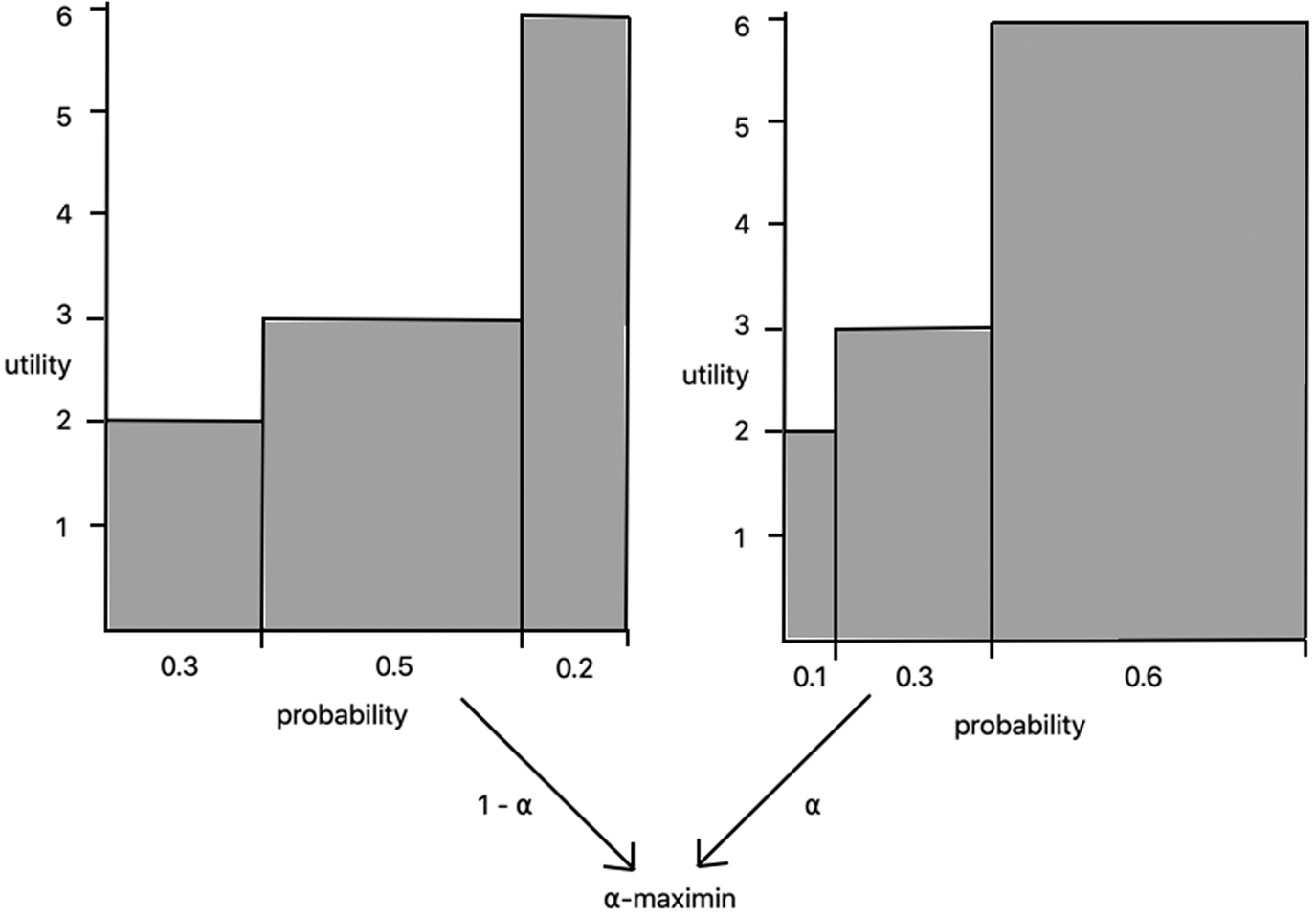
Figure 4. α-maximin.
Attitudes towards risk and attitudes towards ambiguity are conceptually independent. Your attitude towards risk is about how much to weight a consequence whose probability is given. Your attitude towards ambiguity is about what you should do when you are not sure what the true probability is. Thus, it is possible to have any combination of risk-attitudes and ambiguity-attitudes; and we can account for both simultaneously. To combine REU and α-maximin, we can calculate the REU value according to each probability distribution, and then hedge between the minimum and maximum REU, giving the maximum REU weight α, and giving the minimum REU weight 1 − α. We can similarly combine REU with other models of resolving ambiguity by using REU in place of EU.
3. Diversification and hedging
In ethics, we are interested in the good or in moral value, rather than in preferences. But we can make use of the same formal frameworks to rank gambles about the good, since the question of what is morally better under uncertainty has the same structure as the question of what is preferable under uncertainty: what is the relationship between gambles about moral value and their constituent moral values? There are two ways to make use of the formal frameworks about preference to think about moral value, the first of which treats the moral value of outcomes as something to which we have independent access, and the second of which doesn't. The first way is to assume that in moral decisions, the content of a person's preferences is the good: her utility function is equivalent to the moral value function, and she should maximize moral value according to her attitudes towards risk and ambiguity. The second way is to assume that the moral value function is the utility function that represents the preferences of a perfectly moral decision-maker, where these preferences obey a set of axioms that also represent this decision-maker's attitude towards risk and ambiguity.Footnote 20 On either picture, we can use the terms ‘utility’ and ‘moral value’ interchangeably, and ≽ becomes the moral value relation.
We can now apply the idea that there are non-EU attitudes towards both risk and ambiguity to two important questions about charitable giving. The first question: should someone who is concerned only with choosing the best gamble give all of her money to one charity, or should she instead diversify over a number of charities?Footnote 21
We will start by assuming that the status quo is ‘flat’ – contains no risk or ambiguity – in order to see how risk attitudes and ambiguity attitudes make a difference in this simple case. We will then examine the upshots for more realistic cases.
To make things concrete, let us assume you have $200 to distribute to two charities, A and B, and your options are to give $200 to Charity A, to give $200 to Charity B, or to give $100 to each charity. You are interested only in doing what results in the most total good. Let us assume further that the good (represented by utility) is linear in money – each $100 increases the good just as much as the previous $100 – but you have some uncertainty about the effectiveness of each charity: either every $100 donation will increase the good by 1 or every $100 will increase the good by 2. (The uncertainty could come about for a number of reasons, including both uncertainty about the empirical facts and normative uncertainty.) We can represent your choice as among the following three gambles, where ‘SQ’ stands for the status quo, ‘E’ for the event in which each $100 to Charity A will increase the total utility by 2, and ‘F’ for the event in which each $100 to Charity B will increase the total utility by 2:
Give $200 to A (‘2A’): {E̅, u(SQ) + 2; E, u(SQ) + 4}
Give $200 to B (‘2B’): {F̅, u(SQ) + 2; F, u(SQ) + 4}
Give $100 to each (‘AB’): {E̅F̅, u(SQ) + 2; E̅F v EF̅, u(SQ) + 3; EF, u(SQ) + 4}
Since the status quo is flat, it has a single value, u(SQ). If the status quo is itself a gamble, then we can represent it as a single value ‘EU(SQ)’ in expected utility calculations without error, but we cannot do so in the calculations for other theories.
Let us start with the expected utility maximizer who assigns sharp probabilities to E and F. There are only three possibilities here: if p(E) > p(F), then she should strictly prefer 2A to the other options; if p(E) < p(F), then she should strictly prefer 2B; and if p(E) = p(F), then she should be indifferent between all three options:
EU(2A) = u(SQ) + 2 + 2p(E)
EU(2B) = u(SQ) + 2 + 2p(F)
EU(AB) = u(SQ) + 2 + p(E) + p(F)
Notice that for an EU maximizer, the utility value of two gambles – when each gamble is formulated in terms of utility increases to the status quo – is just the sum of their utility values. So whichever gamble is better by itself will still be better in conjunction with another copy of itself. Thus, an EU-maximizer can only prefer diversification (AB) to both other options if taking one copy changes the expected utility value of the two options: if (contrary to the setup here) the good for each dollar spent decreases marginally or if (again contrary to the setup here) the ‘probabilistic good’ of each dollar spent decreases marginally, for example, if the project is an all-or-nothing one for which each additional bit of money increases the probability of success less than the last bit, or if (again contrary to the setup here), as Snowden (Reference Snowden, Greaves and Plumer2019) points out, donations to one charity affect the amount of good that the other charity can do.Footnote 22
What about the risk-avoidant person? Let's take a simple case in which the probability of success is the same for both charities (p(E) = p(F)). If E and F are perfectly correlated, that is, they overlap entirely, then all three acts will be equivalent lotteries – they will yield the same utilities with the same probabilities – so the risk-avoidant person will be indifferent among them. But if they are not perfectly correlated, then the risk-avoidant person will prefer AB to both alternatives;Footnote 23 and she will prefer AB by more the less E and F overlap. She will prefer AB by the most when E and F are anti-correlated, that is, when E obtains only if F does not.Footnote 24 To see this, notice that when p(E̅F) = p(EF̅), AB is a mean-preserving contraction of both 2A and 2B, and AB with less correlation between E and F (i.e., higher values of p(E̅F) and p(EF̅)) is a mean-preserving contraction of AB with more correlation between E and F. (To put the point graphically: 2A and 2B concentrate higher utility in states that are less likely, and AB concentrates not-as-high utility in states that are more likely; the former states will get proportionally less weight – the horizontal rectangle will be shrunk more – than the latter.) The risk-avoidant person would rather hedge her bets on only one of E and F holding than go all-in on either E or F.Footnote 25
It's worth pointing out that for most charities, the conditions for their success will not be perfectly correlated. And indeed, some will be anti-correlated, or close to it. For example, the success of Charity A and the success of Charity B might depend on empirical claims known to be opposed. Consider research for a treatment for Alzheimer's or cancer, where the success of various research programs depends on the causal mechanism behind these diseases. Or the success of Charity A and Charity B may depend on opposing normative claims: one might extend life without improving its quality while the other might improve the quality of life without extending it, where we are unsure whether a longer life or a higher quality of life makes the greater difference to a person's well-being.
Diversification can be rational for the risk-avoidant person even if the two charities aren't exactly equal in terms of their mean utility. If Charity B has a slightly lower expected utility, either because B has a lower probability of being successful or will under its success condition be less successful than Charity A under its success condition, then the risk-avoidant person may still prefer the mixture of A and B (and more so to the extent that E and F are anti-correlated).Footnote 26 In other words, the reasoning that leads to diversification doesn't depend on the two charities being exactly equal from an expected utility perspective.
These points about diversification follow from a more general point: risk-avoidant individuals prefer to hedge their bets. And in the case in which the status quo is flat, hedging one's bets requires diversifying.Footnote 27
We assumed that the status quo is flat; but in typical cases we are uncertain of facts about the world other than which charity will be better. Thus, a more realistic case is one in which the status quo is itself a gamble, namely, one in which the status quo does not have a single utility value u(SQ). Can the results be generalized to this case? Not completely, because the status quo can be such that hedging does not always require diversification. There are three ways in which this could happen, and thus three situations in which a risk-avoidant individual might prefer not to diversify.
First, one of the charities might serve as a kind of insurance against a risk currently present in the status quo. For example, the status quo might be flat except for a 3 utility ‘dip’ in event E. (Maybe both charities involve distributing vitamins, and Charity A's vitamins are effective against a particular disease that may or may not be present in the population, whereas Charity B's vitamins increase the quality of life of an already-healthy population if they are effective.) In this case, giving money to Charity A serves as insurance against E, and so the risk-avoidant individual will prefer to give $200 to Charity A.
Second, if one of the charities has higher expected utility than the other and if the status quo has a particular character – if it has ‘large tails’ and is sufficiently ‘dispersed' in technical senses discussed in Tarsney (Reference Tarsney2020) – then giving $200 to the charity with higher expected utility will stochastically dominate giving $100 to each charity, and thus will have higher risk-weighted expected utility for even the risk-avoidant individual.Footnote 28
Third, if in the status quo you have strong reason to believe that everybody else is giving their money to Charity A, or, more precisely, that the total of everyone else's donations to Charity A will be at least $200 greater than the total of their donations to Charity B, then if you are risk-avoidant you will prefer to give $200 to Charity B, as a way of hedging ‘our’ bet, or of buying insurance against the event in which Charity A is less effective (E̅).
Thus, the set of cases in which diversifying among charities will be required for the risk-avoidant, while wider than the set in which diversifying will be required for EU-maximizers, is still somewhat constrained. Still, the risk-avoidant reason for diversifying is important, both for explanatory and for action-guiding purposes.Footnote 29 Even if the status quo is not flat, many people might assume it is. Alternatively, some people might care about doing the most good with their money in particular, that is, making the most difference, which by definition assumes a flat status quo (no difference made). Thus, we have a candidate explanation for why many people in fact diversify even with respect to small sums of money, and a candidate reason for doing so.
More importantly, for those risk-avoidant individuals or groups who are accounting for all the facts and care about bringing about the best gamble, diversification will still be required when doing so is genuinely the best way to hedge. It will be required in cases that don't meet the above three conditions. And even if we are in a case of a dispersed status quo overall, if someone focuses on helping with respect to a particular issue, cause, or place, the status quo will be less dispersed relative to these. Finally, if we consider interventions large enough to swamp the status quo – such as money donated by all of us collectively – then diversification will still be required.
Let us move next to ambiguity. We will again assume a flat status quo, and consider the choice between 2A, 2B, and AB, as above. We will assume that the individual cannot set a precise value for p(E), p(F), and p(E ∨ F), but instead assigns sets of probabilities; and we will assume that she uses α-maximin, which (recall) takes an average of the minimum EU and the maximum EU. To determine the effects of ambiguity aversion on the choice among these options, we want to know how the spread of possible values of EU(AB) is related to the spread of possible values of EU(2A) and EU(2B).
Taking AB rather than 2A or 2B amounts to betting some on E and some on F rather than betting all on one of these events. Thus, the value of AB for the person who is sensitive to ambiguity depends on the effects of betting some on each event (rather than more on one event) on the spread of possible EU values of the gamble, which in turn depend on how ‘combining’ the probabilities of E and F affects the spread of probabilities of winning at least one of the bets on E or F.
Let Mp(E) stand for the midpoint of the interval representing p(E), and let Sp(E) stand for how spread out the interval representing p(E) is, so that the ambiguity in p(E) is represented by the interval [Mp(E ) − Sp(E), Mp(E) + Sp(E)].Footnote 30 Taking 2A amounts to getting, above the minimum (above u(SQ) + 2): 2 utility if E comes to pass, that is, to an expectation of 2p(E). Taking 2B amounts to getting, above the minimum (above u(SQ) + 2): 2 utility if F comes to pass, that is, to an expectation of 2p(F). Taking AB amounts to getting, above the minimum (above u(SQ) + 2): if E comes to pass, 1 utility; and also, if F comes to pass, 1 utility – that is, to an expectation of p(E) + p(F).
Thus, the value of AB to someone who cares about ambiguity depends on the various values that p(E) + p(F) could take, that is, on the interval [Mp(E)+p(F) − Sp(E)+p(F), Mp(E)+p(F) + Sp(E)+p(F)]. The size of this interval in turn depends on how much the value of p(E) is constrained by the value of p(F), and vice versa, for each probability in the set. If p(E) and p(F) constrain each other a lot, then this interval is small; for example, if p(E) + p(F) = 1 for all p ∊ ${\cal P}$ , then Sp(E)+p(F) = 0, and this interval is simply [1]. If p(E) and p(F) don't constrain each other at all – so that p(E) and p(F) can simultaneously take their lowest (or highest) valuesFootnote 31 – then this interval is as wide as it can be, with Sp(E)+p(F) = Sp(E) + Sp(F). We will assume that Mp(E)+p(F) = Mp(E) + Mp(F); in effect this means that p(E) and p(F) constrain each other in symmetrical ways.Footnote 32
An ambiguity-neutral individual will not strictly prefer diversifying: either she will strictly prefer 2A to all of the other options, or she will strictly prefer 2B to all of the other options, or she will be indifferent among all three options.Footnote 33
What about ambiguity-averse and ambiguity-seeking individuals?
If p(E) and p(F) do not constrain each other's extreme values – if Sp(E)+p(F) = Sp(E) + Sp(F) – then diversification cannot be preferred, for any value of α.Footnote 34 An intuitive way to think about this is that if p(E) and p(F) do not constrain each other, then the ambiguity present in the gambles together is just their combined ambiguity. Thus, whichever gamble the ambiguity-averse individual prefers when taken by itself, that gamble will also be preferred no matter which other gamble she already holds (and similarly for the ambiguity-seeking individual). Diversifying doesn't reduce overall ambiguity.
However, if p(E) and p(F) do constrain each other – if Sp(E)+p(F) < Sp(E) + Sp(F) – then pairing A with B does reduce ambiguity, and so diversifying can be preferred to putting all of one's money towards one gamble.Footnote 35 To take an extreme example, while I might not know whether p(E) is 0.25 or 0.75, and I might not know whether p(F) is 0.25 or 0.75, I might know that if p(E) is 0.25 then p(F) is 0.75, and vice versa, that is, it might be that all the probability functions in my set have p(E) + p(F) = 1. If so, then when I already hold A, taking B provides a kind of insurance against the possibility of A having a bad probability distribution. And as in the risk case, diversifying can be preferred even if one of the charities is by itself slightly preferred to the other.
Thus, the results for ambiguity-aversion and risk-avoidance are similar, but whereas diversification is more apt to be preferred in the case of risk-avoidance when the possible events constrain each other (when their probabilities are not independent), diversification is more apt to be preferred in the case of ambiguity-avoidance when the possible probabilities constrain each other.
In cases of charitable giving, it is not uncommon for the probabilities to constrain each other. Consider the examples of anti-correlation discussed in the case of risk-avoidance, in which the success of Charity A and the success of Charity B depend on opposing empirical or normative claims. If claims are anti-correlated, then their probabilities will often constrain each other (for example, if p(E v F) is fixed, then if p(E & F) = 0, when p(E) is high, p(F) will be low). Alternatively, probabilities may constrain each other if, for example, the highest probability of E and the highest probability of F are based on opposing scientific models. Diversifying in the case of ambiguity is similar to diversifying in the case of risk: whereas in that case, it was rational for the risk-avoider to hedge between different ways the world could turn out, in this case, it is rational for the ambiguity-averter to hedge between different ways the probabilities could be.
When the status quo is flat, hedging between ambiguous gambles makes sense if the individual is ambiguity-averse and if the probabilities constrain each other. However, as in the case of hedging between risky gambles, this fact only holds if the status quo is not itself ambiguous in a particular way. If, for example, donating to Charity A reduces the ambiguity in the world, by hedging against already existing ambiguity, then one might prefer to donate $200 to Charity A rather than to diversify. Or, again, if one knows that many people are donating to Charity A, then one should, if one is ambiguity-averse, donate $200 to Charity B, to reduce the overall ambiguity. So, as in the case of risk-avoidance, ambiguity-aversion won't explain all cases of diversifying; nor will diversifying always be rationally required for ambiguity-averse individuals. However, we have again hit upon a new explanation for diversification, as well as a set of circumstances in which ambiguity-averse individuals ought to diversify. Insofar as diversification looks like buying insurance against the probability distribution turning out a certain way, it's going to be a good thing for the ambiguity-averter. And insofar as it doesn't, it won't be.
4. Existential risk mitigation vs. health amelioration
We have seen how risk-avoidance and ambiguity-aversion can lead to diversification in charitable giving. Let us turn next to the choice between different types of programs to give money to. On the one hand, there are programs which have well-known, high probability, positive effects in exchange for relatively small amounts of money. Consider, for example, the Against Malaria Foundation, which provides insecticidal nets, or Give Directly, which gives money directly to people in need.Footnote 36 Let us define a steady increase program as follows, simplifying ‘high probability’ to ‘probability 1’ for ease of exposition:
Steady Increase Program (SIP): A given small dollar amount raises the utility of the status quo by a fixed, small utility value in every state of the world.
On the other hand, there are programs which have a small probability of doing a massive amount of good, but for which: (1) donating a small amount of money serves primarily to slightly increase the probability of some massive difference in how good the outcome is; and (2) that probability is ambiguous. For example, consider the International Campaign to Abolish Nuclear Weapons (ICAN) or a program advocating for increased precautions against pandemics, both of which have a small probability of causing us to avoid a massively bad outcome; or consider SpaceX's program to colonize Mars, which has a small probability of bringing about a massively good outcome.
There are two ways to slightly increase the probability of some massive utility difference: we could decrease the probability of a massive amount of bad or increase the probability of a massive amount of good. (Here, ‘bad’ just means a possible state that is relatively much worse than most other possible states, and ‘good’ means a possible state that is relatively much better than most other possible states.) Thus, we can distinguish two types of “small probability of large utility” programs. One program we can call existential insurance: in the status quo, some massively bad event might happen, but its probability is small. Existential insurance lowers the chance of that massively bad event, or makes things not go poorly if that event comes to pass; ICAN and the program advocating for pandemic precautions are examples.
Let us define existential insurance as follows:
Existential Insurance (EI): Whereas the status quo currently contains as a possibility a massively bad event (an event with much lower utility than the rest of the status quo) with a small probability, a given dollar amount lowers the probability of getting that utility value.
One special case of existential insurance is the case of lowering the probability of the bad event to 0.
There are also programs that we might call an existential lottery ticket. An existential lottery ticket raises the probability of some currently improbable massively good event. Examples include SpaceX or the transhumanist program dedicated to extending individual lives indefinitely.Footnote 37 We can define an existential lottery ticket as follows:
Existential Lottery (EL): Whereas the status quo currently contains as a possibility a massively good event (an event with much higher utility than the rest of the status quo) with a small probability, a given dollar amount raises the probability of getting that utility value.
One special case of the existential lottery is the case of raising the probability of the “possible” good event from 0.
In this section, we are interested in how different attitudes towards risk and ambiguity should affect our giving to these three types of causes. To isolate the effects of risk and ambiguity from other effects, we will consider a case in which an example of each type has the same expected utility. (This implicitly assumes that there are no infinite values involved.) We will then ask what happens if we take a non-EU attitude towards risk or ambiguity or both.
Let B refer to the bad event with massively low utility and low probability (e.g., nuclear war), G refer to the good event with massively high utility and low probability (e.g., colonizing other galaxies), and N refer to the neutral event in which neither happens. To give some definite values, we will say that in the status quo, the bad event has utility −100, the neutral event has utility 0, and the good event has utility 100. Furthermore, the steady increase program adds just over 1 utility in the neutral event (we are assuming that it doesn't add anything in the good or bad event). The existential insurance lowers the probability of the bad event by e and the existential lottery ticket raises the probability of the good event by t. So we have:
SQ = {−100, p(B); 0, p(N); 100, p(G)}
SIP = {−100, p(B); 1/p(N), p(N); 100, p(G)}
EI = {−100, p(B) − e; 0, p(N) + e; 100, p(G)}
EL = {−100, p(B); 0, p(N) − t; 100, p(G) + t}
We will begin by assuming that we can give e and t definite values; we will assume e = t = 0.01. When one is comparing actual Steady Increase Programs to Existential Insurance to Existential Lottery programs, the utility numbers may be much greater in magnitude and probability numbers much smaller in magnitude than the ones in our example; however, very large and very small numbers can be difficult to conceptualize, so I'm using this toy example to make the effects of risk and ambiguity easier to understand.
Under these assumptions, the expected utility maximizer is indifferent between SIP, EI, and EL. (It is easy to see that EU(SIP) = EU(EI) = EU(EL) = EU(SQ) + 1.) All three gambles involve adding 1 expected utility to the status quo, spread out in different ways: SIP adds approximately 1 utility nearly everywhere; EI adds 100 utility to 0.01 of the states in the bottom part of the gamble; and EL adds 100 utility to 0.01 of the states in the top part of the gamble. (If p(B) = e, then EI eliminates the worst possibilities, and if p(G) = 0, then EL introduces new best possibilities.)
Now let us consider risk-attitudes. The strictly risk-avoidant person puts more weight on relatively worse scenarios and less weight on relatively better scenarios. Given 1 utility to distribute, she prefers putting as much as possible in the worst possible states. Thus, the strictly risk-avoidant person will strictly prefer the existential insurance to the steady increase program, and strictly prefer the steady increase program to the existential lottery.Footnote 38 The strictly risk-inclined person will have the opposite preferences, since she cares more about what happens in better states than in worse states (Table 1).
Table 1. Attitudes towards risk

To consider ambiguity-attitudes, recall that both existential programs can involve uncertainty about the effects of one's contribution. To capture this, instead of fixing e and t at 0.01, they will be represented by an interval centered on 0.01 with spread 0 < s ≤ 0.01: e ∈ [0.01 − s, 0.01 + s], t ∈ [0.01 − s, 0.01 + s]. This captures the idea that although these programs might change the probability of the massively bad or massively good thing by 0.01, they might instead (optimistically) change it by 0.01 + s, or they might instead (pessimistically) change it by 0.01 − s.
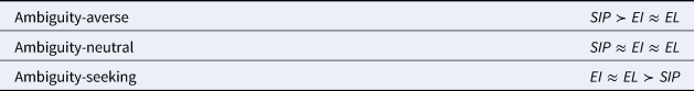
For the ambiguity-avoidant person, the ambiguity involved in both the existential insurance and the existential lottery makes these programs worse than the steady increase program. However, since EU is insensitive to where utility is added, a theory of ambiguity-preferences based on averaging the minimum and maximum EU will treat ambiguity in worse states equivalently to ambiguity in better states.Footnote 39 Therefore, if the ambiguity in both gambles is the same (the spread is equally wide, and concerns the same amount of utility), the ambiguity-averse individual will be indifferent between the existential insurance and the existential lottery. Thus, the ambiguity-averse person strictly prefers the steady increase program to both the existential insurance and the existential lottery, and is indifferent between the latter two; and by analogous reasoning, the ambiguity-seeking person strictly disprefers the steady increase program to the existential insurance and the existential lottery, which she is indifferent between (Table 2). (It might be, contra the toy example, that there is more ambiguity involved in the existential lottery than in the existential insurance, or vice versa, in which case the ambiguity-averse person will prefer the gamble with less ambiguity; the point is that the effects of ambiguity do not depend on whether a gamble is insurance or a lottery.)
Table 2. Attitudes towards ambiguity.
We can also consider what happens when we combine attitudes to risk with attitudes to ambiguity.Footnote 40 The possibilities are listed in Table 3.Footnote 41 Notice that for many combinations of attitudes, there are multiple possibilities. For example, if you're risk-avoidant and ambiguity-averse, then the existential lottery is made worse than the other choices by risk-avoidance, and made not better by ambiguity-aversion; but since risk-avoidance makes the existential insurance preferable to the steady increase program and ambiguity-aversion does the opposite, which is preferable overall will depend on which attitude is more severe.
Table 3. Preferences with different attitudes
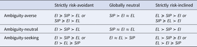
It would be unrealistic, of course, to assume that Steady Increase Programs, Existential Insurance Programs, and Existential Lotteries in general have the same average utilities, and the orderings in Figure 5 are only guaranteed to hold if they do. When the programs do not have the same average utilities, “≻” and “≺” and “≈” instead represent the direction of change in value based on risk and ambiguity attitudes; for example, for an ambiguity-averse and risk-avoidant individual, Steady Increase Programs will go up in value relative to Existential Lottery Programs, in contrast to how an EU-maximizer evaluates these.
One surprising fact to note is that the Steady Increase Program can only look better than both Existential Programs if one is ambiguity-averse; and even then, it may not, if one is sufficiently risk-avoidant or risk-inclined. In other words, caring about risk (in either direction) won't provide reason to pick the option that makes a difference for certain, since the person who avoids risk will rather have insurance, and the person who seeks risk will rather have a lottery. This surprising fact, of course, rests on the assumption that the programs are equally good on average. Furthermore, while I have provided canonical examples of Existential Programs, the claim that the relevant good or bad events in these examples are genuinely much better or worse than the status quo (which includes people in poverty or with unmet health needs or prematurely dying) rests on a particular aggregative theory of the good, among other assumptions. So application to real-world choices – deciding to give money to increase pandemic precautions or to reduce cases of malaria, for example – rests on carefully considering whether these features hold.
5. What attitudes should we adopt in our charitable giving?
We've explored how we should apportion our giving when we adopt different attitudes towards risk and ambiguity. But which attitudes should we adopt? There are several possibilities for answering this question, and this final section will explain where the decision points lie.Footnote 42
The first decision point is whether charitable giving should be thought of as an individual or collective enterprise: am I trying to do the most (risk-weighted and ambiguity-resolved expected) good possible with my money, or are we trying to do the most (risk-weighted and ambiguity-resolved expected) good possible with our money? If it should be thought of as an individual enterprise, then each individual giver should hold fixed what others are doing – treat others’ behavior as part of the status quo – and concentrate on the difference her donations make to the good. According to this view, we should then ask: which risk-attitudes and ambiguity-attitudes should an individual adopt when making decisions whose purpose is to bring about good for others? There are three possible answers. First, that she should adopt her own attitudes. Second, that she should adopt the others’ attitudes, however ‘their attitudes’ is to be defined for the collective she is trying to help.Footnote 43 And third, that she should adopt some particular, objective risk-attitude and ambiguity-attitude. Uncertainty in the status quo will be, for the typical giver, more pronounced under the view that charitable giving is an individual enterprise, since the amount of money any particular giver is giving is dwarfed by others’ contributions.
If charitable giving should be thought of as a collective enterprise, then we should treat the status quo as including only contingencies that exist apart from our collective intervention, and ask about the difference that our collective charitable giving will make to the (risk-weighted and ambiguity-resolved expected) good. There are again three different ways to think about which attitudes we should adopt when making decisions whose purpose is to bring about good for others, echoing those above. First, that we should adopt our own attitudes, where ‘our attitudes’ is determined by aggregating in some way, just as we might aggregate if we disagree about the probabilities. Second, that we should adopt the attitudes of the others we are trying to help. Finally, that we should adopt some particular, objective attitudes. This last option will yield a different recommendation than under the ‘individual’ view, since the choices will be about total giving rather than individual giving holding fixed what others give, and thus both the characterization of the status quo and the amount of money under consideration will be very different.
Many ways of resolving these choice points will lead to risk-avoidance, ambiguity-aversion, or both. Since many people in fact have these attitudes, if we use the attitudes of either the giver or the ones being helped, we are apt to land on risk-avoidant and ambiguity-averse choices. (Though I note that the common ‘S-shaped’ risk profile will also lead to risk-inclination in small probabilities, such as in the case of the existential lottery.) Likewise, if we think there is an objective requirement on how to set these attitudes when making choices that affect others, then there may be a good case to be made that that requirement is risk-avoidance or ambiguity-aversion.Footnote 44
More will have to be done to say which attitudes we should adopt in our charitable giving, and exactly which charities we should give to. But my hope is that this article has shed light on exactly why and how these attitudes matter when figuring out how to do the most good.
Acknowledgments
This article benefited greatly from comments by Jacob Barrett, Hilary Greaves, Andreas Mogensen, Christian Tarsney, Teru Thomas, David Thorstad, Hayden Wilkinsen, and Timothy Williamson; from comments by the editor of this journal and two anonymous referees; and from discussions at the Global Priorities Institute in Oxford in 2019, where it was first presented as the Derek Parfit Memorial Lecture in 2019.
Competing interests
The author(s) declare none.


 Open access