Introduction
The presence of weeds continues to be one of the most yield-limiting factors and is the cause of up to 39% of soybean [Glycine max (L.) Merr.] yield loss in the midwestern region (USDA-NASS 2014). According to a questionnaire survey conducted by the Weed Science Society of America in 2016, horseweed [Conyza canadensis (L.) Cronquist] was the most common and troublesome weed in Ohio soybean production (Van Wychen Reference Van Wychen2016). A single C. canadensis plant can produce up to 200,000 seeds, capable of spreading as far as 500 m from the seed source (Bhowmik and Bekech Reference Bhowmik and Bekech1993; Dauer et al. Reference Dauer, Mortenson and VanGessel2007). Additionally, C. canadensis can exist as a summer annual, winter annual, or biennial (Buhler and Owen Reference Buhler and Owen1997). This complicates the control of C. canadensis, as contamination can come from multiple sources (temporally and spatially) and germination is unpredictable.
An increase in the number of herbicide-resistant weeds and their spread in Ohio have made weed control efforts more complex and expensive. Beyond innate biological advantages, herbicide resistance has made C. canadensis increasingly difficult to control. Conyza canadensis populations in Ohio have exhibited resistance to acetolactate synthase (ALS) inhibitors (site 2), 5-enolpyruvylshikimate-3-phosphate synthase (EPSPS) inhibitors (site 9), and multiple resistance to both ALS and EPSPS inhibitors (Heap Reference Heap2018). Failure to control C. canadensis can cause soybean yield loss of up to 940 kg ha−1 in Ohio soybean production, a value of roughly $320 ha−1 (Loux et al. Reference Loux, Doohan, Dobbles, Johnson, Young, Legleiter and Hager2016).
On-site surveys of weed populations in growers’ fields provide information on the relative occurrence and density of weeds that can be useful to growers in that region (Loux and Berry Reference Loux and Berry1991). While national surveys can be beneficial, it is important to also conduct higher-resolution surveys, as weeds that are common and troublesome in larger regions of the country are not always the most problematic in a certain state (Rankins et al. Reference Rankins, Byrd, Mask, Barnett and Gerard2005). These surveys can also be used to monitor temporal shifts in species within selected geographic areas (Rankins et al. Reference Rankins, Byrd, Mask, Barnett and Gerard2005). Landowners, producers, extension educators, and weed scientists all have something to gain from the data generated by weed surveys, as they can aid in the management of weed issues by monitoring the movement of problem weeds and forecasting areas susceptible to infestations (Korres et al. Reference Korres, Norsworthy, Bagavathiannan and Mauromoustakos2015). Maps are helpful tools in examining the geographic distribution and spread of weed species, which can be supplemented by information on species abundance and infestations, to illustrate regional differences and predict species occurrences (Hanzlik and Gerowitt Reference Hanzlik and Gerowitt2016).
Geostatistics is a valuable tool in the analysis of data in agricultural sciences. It has been used in fields such as soil science, entomology, ecology, and hydrology. This type of analysis allows scientists to evaluate relationships between variables and regionally distribute these variables into space and time, versus each variable being considered random under a probability distribution (Gassner and Schnug Reference Gassner and Schnug2006). Geographic information systems (GIS) and associated open-source mapping software systems have increased the ease of use and accessibility to this type of analysis and have allowed for the expansion of geostatistics into several disciplines. Historically, geostatistics and GIS have been used in the discipline of weed science primarily to model patterns of weed populations and spatial arrangement at the field level (Cardina et al. Reference Cardina, Johnson and Sparrow1997; Colbach et al. Reference Colbach, Forcella and Johnson2000; Dille et al. Reference Dille, Milner, Groeteke, Mortensen and Williams2002; Johnson et al. Reference Johnson, Mortensen and Gotway1996). This methodology can be useful in scouting, sampling, and mapping weed populations within a single field. The ability to predict the distribution of weeds with a certain level of accuracy could lead to site-specific management (Wiles and Schweizer Reference Wiles and Schweizer2002; Wyse-Pester et al. Reference Wyse-Pester, Wiles and Philip2002). GIS have also been used to model herbicide movement, map pesticide leaching potential, forecast impact of climate change on invasive plants, and predict distribution of invasive weed species in non-cropland habitats based on spatial variables (Hornsby Reference Hornsby1992; Jarnevich et al. Reference Jarnevich, Holcombe, Barnett, Stohlgren and Kartesz2010; Mitchell et al. Reference Mitchell, Pike and Mitasova1996; Vanderhoof et al. Reference Vanderhoof, Holzman and Rogers2009). This type of analysis could also be useful in identifying spatial and temporal trends of problem weeds on a larger scale in agricultural production (Kalivas et al. Reference Kalivas, Vlachos, Economou and Dimou2012) but is often limited by a lack of geospatial data on weed distribution (Mueller-Warrant et al. Reference Mueller-Warrant, Whittaker and Young2008). Generating a database of weed frequency and distribution utilizing GIS and associated analysis software could assist in tracking and managing problematic weeds (Fletcher and Reddy Reference Fletcher and Reddy2018).
The objectives of this research were to: (1) determine the frequency, level of infestation, and distribution of C. canadensis in soybean fields in the top soybean-producing counties in Ohio over 5 yr; and (2) identify any significant spatial clusters or movement trends over time. The overall goal of this study was to provide weed scientists, county educators, and growers with information on the locations and distribution of C. canadensis to aid in planning educational efforts and weed management programs.
Materials and Methods
Survey Design
A survey of soybean fields in 49 of 88 Ohio counties was conducted annually each fall from 2013 to 2017, just before soybean harvest (Figure 1). Conducting the survey at this time reflected the final effect of all control measures applied during the season and facilitated observation from a distance of plants with seed above the soybean canopy, which were of primary interest. Routes were created using Google Earth (Google, Mountain View, CA) with the objective of driving diagonal transects across each county (Supplementary Figure S1). These routes were loaded onto a Garmin GPS (Garmin International, Olathe, KS) system for navigation. To account for the predominant corn (Zea mays L.)–soybean crop rotations, the same routes were driven for 2 yr and then adjusted based on number of fields passed and roads available. The state was divided into nine regions based on the Ohio Agricultural Statistics Districts used by the USDA (USDA-NASS 2018). Of these regions, 49 counties in six regions were surveyed annually. Each region was evaluated in a single day. To capture as many unharvested fields as possible, regions were evaluated sequentially each year from most to least dry, based on the National Drought Mitigation Center’s map of Ohio (Bathke Reference Bathke2017).
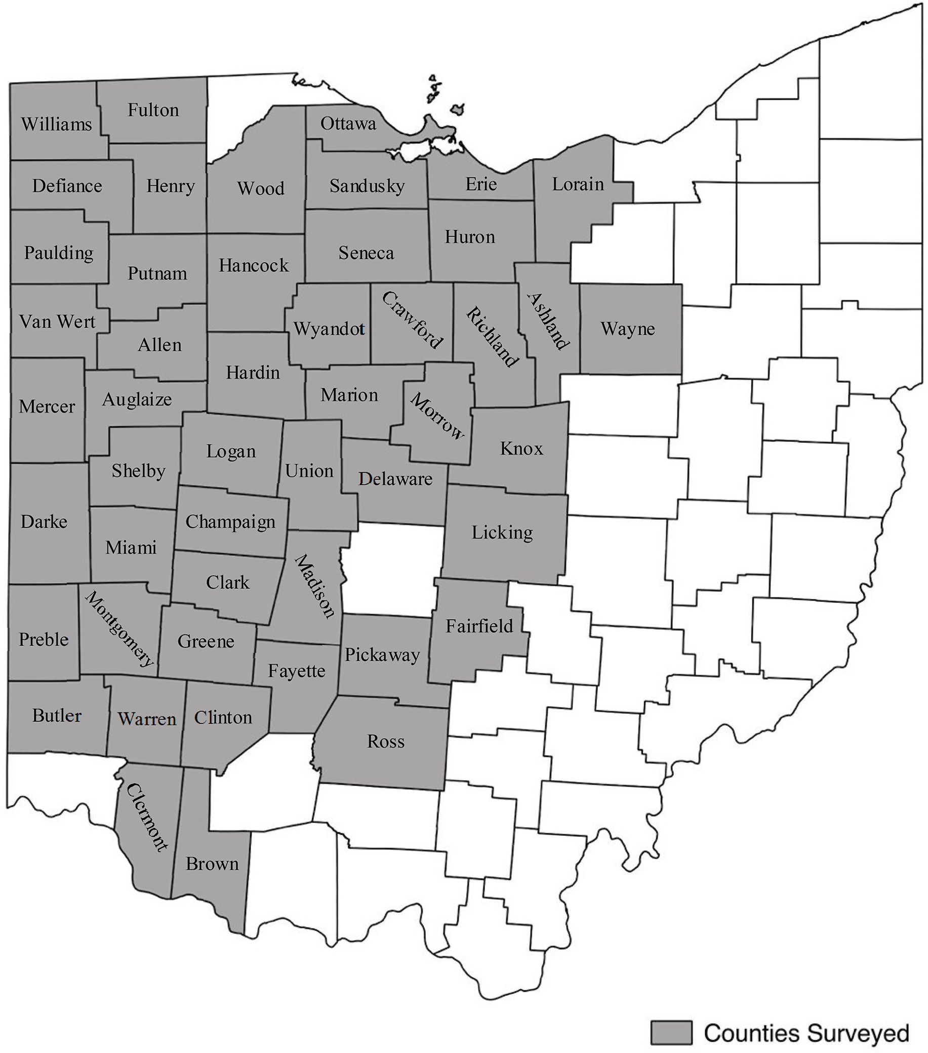
Figure 1. Ohio counties included in the survey, 2013 to 2017.
Counties with at least 4,050 ha of soybean production were surveyed, mostly located in the central, northern, and western regions of the state. Counties made up of primarily large metropolitan areas and those with less than 4,050 ha of soybean production were excluded from this survey. This threshold represents the estimated lowest number of hectares necessary to reasonably capture representative C. canadensis levels using the described driving survey methodology. The counties that were included in the survey ranged anywhere from 16,200 to 65,200 ha of soybean production in 2017. The average soybean production for counties surveyed in 2017 was 38,700 ha, and the median was 39,200 ha (USDA-NASS 2018). The excluded counties in 2017 ranged from 760 to 17,000 ha of soybean production, with a median value of approximately 7,000 ha. Of the excluded counties where soybean production was recorded, the median soybean production was 6,700 ha (USDA-NASS 2018). It should be noted that many counties in the regions not surveyed do not have data for soybean production as a result of negligible hectares. The few counties in these regions that have soybean production above the indicated threshold of 4,050 ha were not surveyed. There was a small window of time when weeds were a sufficient size to rate before harvest began. As such, priority was given to regions with counties that had consistently sufficient soybean production.
Visual evaluations of C. canadensis frequency and population density were measured for each soybean field encountered. The specific fields evaluated varied over years due to crop rotation and changes in driving routes. A stratified sampling procedure was utilized, and each field was given a single rating. These visual evaluations were based on visibility of C. canadensis above the soybean canopy and were assessed from the vehicle with the aid of binoculars. The entirety of the field that could be observed was considered in the rating, and the most prevalent C. canadensis distribution within the field (or average) was the main consideration in determining the designated field rating. The purpose of using this driving survey methodology was to cover as much ground as possible within the given time frame, prioritizing quantity of fields evaluated over small-scale precision of ratings. Fields in Ohio are not as large as in many other areas of the Midwest, and for the majority it was possible to observe most of the field. A nominal rating scale of 0 to 3 was used to classify C. canadensis population levels, based on visual estimates from the field edge. Rating levels were: 0, not present; 1, single, isolated weeds scattered in the field; 2, clustered groups dispersed throughout the field; and 3, dense, widespread clusters, indicative of an infestation (Supplementary Figure S2). Based on the authors’ experience with grower management of herbicide-resistant C. canadensis, these levels can also be considered to represent the following: 0, effective management; 1, effective management but a few escapes ; 2, substandard management with some seed production likely to have minor effects on crop yield; and 3, completely ineffective management with substantial seed production and some effect on crop yield or harvestability (Supplementary Figure S3).
A total of approximately 3,400 to 4,900 fields were evaluated each year (Table 1). The goal of this survey was to provide a broad understanding of the location and density of C. canadensis populations within the state at the county level. The location and density of smaller C. canadensis plants below the canopy that emerge late and typically lack seed and specific location of C. canadensis within the field or county were compromised to provide a larger data set on a greater number of fields that covers a larger area throughout the state.
Table 1. Frequency of Conyza canadensis present by rating level in surveyed soybean fields just before harvest, 2013 to 2017.

Data Analysis and Presentation
Quantum geographic information system (OSGeo, Beaverton, OR) software was used to create gradient maps of Ohio demonstrating the movement of C. canadensis by rating at the county level from year to year and also to illustrate the results from the spatial data analysis software, GeoDa (CSDS, Chicago, IL). GeoDa was used to identify notable amounts of C. canadensis populations, or lack thereof, by rating and county in relation to surrounding counties. To determine whether the changes in C. canadensis populations over time were spatially clustered, the univariate local Moran’s I test was performed to identify spatial hot spots of interest, a means of autocorrelation (Anselin Reference Anselin1995). This tested the number of fields at a certain rating in a county compared with neighboring counties using the queen’s case contiguity (or Moore neighborhood) by running a number of conditional permutations, a method of numerically testing for significance that yields a pseudo significance value (Anselin Reference Anselin1995). This method of spatial autocorrelation has been utilized to determine whether the presence of a condition in one location makes the condition more or less likely to occur in surrounding locations (Sawada Reference Sawada2009). It is a statistical means of assessing whether the presence of C. canadensis in one county is dependent on or independent of its presence in neighboring counties.
The parameters for this evaluation were set to 99,999 permutations at a significance level of 0.01 to avoid false findings as a result of the pseudo P-values and multiple comparisons (Anselin Reference Anselin2017). Significant observations in the classical sense were referred to as points of interest, which is more appropriate for this type of analysis (Anselin Reference Anselin2017; Efron and Hastie Reference Efron and Hastie2016). The output was a number of local indicators of spatial association (LISA) maps revealing the core clusters of interest or outliers of C. canadensis populations in the state, as well as a Moran’s I value for the model. The Moran’s I value can be used to detect spatial relationships; the cutoff is typically a value greater than 2k/n (k = number of explanatory variables; n = sample size), which in this case was 0.082. Positive I values indicated spatial clusters with similar high or low values, whereas negative I values indicated cores with neighbors having contradictory high or low values (Anselin Reference Anselin1995). Regression analyses were also performed to evaluate the relationship between Ohio C. canadensis populations and time at each rating level. This was done in SAS v. 9.4 (SAS Institute, Cary, NC) using the REG procedure.
County data are presented here in a classification system consisting of four categories: high–high (HH), high–low (HL), low–high (LH), or low–low (LL). Counties classified as HH were those with a high number of fields at a given rating for C. canadensis, surrounded by counties that also had a high number of fields with C. canadensis at that rating. HL counties had a high number of fields relative to neighboring counties that had low levels of C. canadensis at a given rating. LH counties were those with a low level of C. canadensis fields, surrounded by counties with higher levels of C. canadensis given the same rating. LL counties were those with a relatively low level of C. canadensis and were surrounded by counties that also had a low number of fields with C. canadensis given the same rating.
Results and Discussion
Conyza canadensis occurred at least once in each of the 49 counties surveyed across the state in all years and was observed in 24% to 38% of fields overall among years (Table 1). The number of fields assigned a rating of 1 was highest in 2015 at 27.2% and decreased overall in the later years of the survey (Table 1). The highest frequency of level 2 C. canadensis populations occurred in 2015 at 7.5% but remained relatively constant throughout the years. Infestations, or fields assigned a rating of 3 were also highest in 2015 at 2.9%, which coincided with the highest overall frequency of C. canadensis at 38% of total fields. The lowest percentage of fields with C. canadensis present was in 2017 at 24%, but this coincided with the second-highest percentage of infestations, 2.3%. The number of C. canadensis populations at each rating level per county was variable from year to year, with some counties having at least two infestations per year and some counties having no more than one infestation per year.
2013
Conyza canadensis was observed in 35% of the surveyed soybean fields in 2013, with an infestation rate of 1.9% (Table 1). The number and distribution of C. canadensis populations were variable across the state. Most counties seemed to have between 10 and 40 fields designated a rating of 1, with higher-frequency counties located mainly in the central part of the state (Figure 2). According to the LISA map and the Moran’s I, four counties were identified as points of interest at the 1 rating. Madison and Union were HH counties, and Butler and Preble were LL counties (Figure 3; Table 2). Similarly, most of the counties with a greater number of fields rated 2 seemed to be in the west-central part of the state (Figure 4). Two counties were identified as points of interest at the level 2 rating; Logan and Champaign counties were HH counties (Figure 5; Table 2). Fields given a rating of 3 had fairly even numbers across the state, with Fulton County having a much greater number of fields at this rating than any other county (Figure 6). Auglaize County was identified as an LL county. At 10 fields, Fulton County had the highest number of infestations in 2013, or 12% of the fields surveyed in the county. Fulton County was identified as a point of interest in 2013 as an LL county for C. canadensis infestations (Figure 7; Table 2).

Figure 2. Gradient of the distribution of fields with single, isolated Conyza canadensis plants (level 1 rating) in Ohio soybean fields based on the number of infestations per county each year.

Figure 3. The cores and neighbors of significant clusters of fields with single, isolated Conyza canadensis plants (level 1 rating) in Ohio soybean fields.
Table 2. Significance of fields at the respective rating levels by year from univariate local Moran’s I test.


Figure 4. Gradient of the distribution of fields with clustered groups of Conyza canadensis (level 2 rating) in Ohio soybean fields based on the number of infestations per county.

Figure 5. The cores and neighbors of significant clusters of fields with clustered groups of Conyza canadensis (level 2 rating) in Ohio soybean fields.

Figure 6. Gradient of the distribution of fields with Conyza canadensis infestations (level 3 rating) in Ohio soybean fields based on the number of infestations per county.

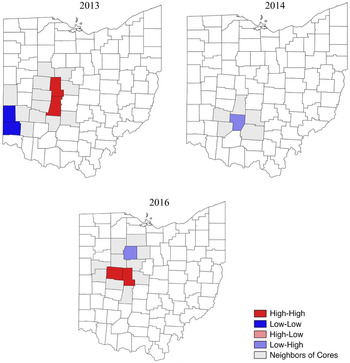
Figure 7. The cores and neighbors of significant clusters of Conyza canadensis infestations (level 3 rating) in Ohio soybean fields.
2014
Conyza canadensis infestations occurred in 1.9% of total fields in 2014 and were present in 32% of fields (Table 1). Fields at the level 1 rating seemed to be mostly in the range of 10 to 30 per county, with most of the counties with higher ratings centrally located (Figure 2). One county of interest was identified at the 1 rating. Fayette was an LH county for fields rated 1 for C. canadensis (Figure 3; Table 2). The south and west-central regions of the state had more counties with a higher number of fields given a rating of 2 (Figure 4), and five counties were identified as points of interest. Union, Champaign, and Miami were HH counties, and Van Wert and Allen were LL counties (Figure 5; Table 2). Infestations also seemed to be more frequent in the central and lower regions of the state in 2014 (Figure 6). Three spatial clusters of interest were illustrated by the LISA map, the cores of which were Clermont, Montgomery, and Logan counties (Figure 7; Table 2). Both Clermont and Montgomery were identified as LH cores. This was logical, as the southern region of the state appeared to have a higher number of infestations than the northern region, leaving these two counties that had a lower number of infestations as outliers. Logan County was defined as an HL county, having a high number of fields with infestations relative to surrounding counties in the west-central part of the state.
2015
The 2015 survey resulted in the highest overall frequency and infestations of C. canadensis at 38 and 2.9%, respectively (Table 1). The number of fields given a rating of 1 in 2015 were evenly distributed throughout the state. Counties appeared darker overall than in previous years, indicating more fields given a rating of 1 (Figure 2). Paulding County had a much higher number of fields given a rating of 1 relative to other counties. There were no counties designated as points of interest at the 1 rating in 2015 (Table 2). Similar to the 1 rating, a rating of 2 was given to more fields in 2015 than in previous years. No counties were identified as points of interest according to the LISA maps or Moran’s I value (Figure 4; Table 2). In 2015, the northwest region of Ohio experienced an exceptionally high frequency of C. canadensis infestations compared with the rest of the state (Figure 6). Williams, Henry, and Wood were counties of interest in the HH category in 2015 (Figure 7; Table 2).
2016
Counties with a greater number of fields given a rating of 1 seemed to be in the central and more northern regions of the state in 2016 (Figure 2). Three counties of interest were identified at the 1 rating level. Union and Logan counties were HH counties, and Wyandot was an LH county (Figure 3; Table 2). Similarly, the counties with the most fields at the level 2 rating were located in the central and northern regions of the state (Figure 4). One county of interest was identified at the level 2 rating in 2016, with Champaign found to be an HH county (Figure 5; Table 2). There seemed to be many counties with a higher frequency of infestations, or a level 3 rating, that were dispersed evenly across the state (Figure 5). Only one county of interest, Ross, was identified in 2016 as an HL county (Figure 7; Table 2).
2017
In 2017, fields assigned a rating of 1 were evenly dispersed throughout the state. Most counties were somewhere in the range of 10 to 20 fields with a rating of 1 (Figure 2). Fields assigned a rating of 2 were more frequent in the central and northern regions of the state (Figure 4). In general, there were fewer counties with a high number of infestations. However, there were more counties with a midlevel frequency of infestations compared with previous years, during which most counties had lower numbers of infestations (Figure 6). While there were fewer overall infestations on a county level, there was a higher number of infestations more evenly distributed throughout the state. No counties were identified as points of interest at any C. canadensis rating level in 2017 (Table 2).
The results of the univariate local Moran’s I displayed by the LISA maps are supported by the gradient maps generated by QGIS, in that counties designated as points of interest often had a much higher or lower number of infestations in comparison to neighboring counties. Lighter shades indicate a lesser frequency of infestations, and increasingly darker shades illustrate more frequent infestations. Looking at the overall frequency of C. canadensis at each rating level, there does not appear to be a trend in the increase or decrease of C. canadensis populations from 2013 to 2017. However, there was an overall, gradual darkening from year to year on the gradient maps of Ohio in terms of the lower to middle levels of infestations. Regression analyses were used in an attempt to understand the change in C. canadensis populations at the various ratings over the years. While the regressions were not significant, they confirmed that the overall survey trend in terms of the years presented was a decrease in C. canadensis present in fields as isolated plants, a static number of fields with C. canadensis in clusters, and an increase in the number of fields with infestations (Figure 8).

Figure 8. Regression results of fields with single, isolated Conyza canadensis plants (level 1 rating; P = 0.27), clustered groups of C. canadensis (level 2 rating; P = 0.89), and infestations (level 3 rating; P = 0.26) by year. MSE, mean square error.
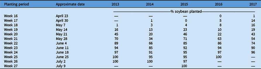
The lowest total C. canadensis encounters for the sum of all ratings occurred in 2017, but that year also had the second-highest frequency of infestations among years. While there may have been a lower overall frequency of C. canadensis throughout the state (Table 1), the areas in which it was present were also more likely to have infestations. These results suggest that overall during these 5 yr, growers may have implemented effective programs for the management and control of C. canadensis, reducing its overall frequency and presence in Ohio soybean production fields. Adoption of new soybean traits, including glufosinate tolerance, increased over this time period as well and likely contributed to improved control, especially in fields with low population levels of C. canadensis. Sales of this herbicide trait in soybean grew from 2014 to 2018 and now make up nearly 20% of soybean market share (Unglesbee Reference Unglesbee2018). Beyond new technology, contrasting management efficacies may have impacted frequency and distribution of C. canadensis over time resulting in: (1) an overall reduction in fields rated a level 1 due to the adoption of more effective management practices or soybean systems; and (2) the constant or increasing frequency of fields rated at a level 2 or 3 due to a failure by some growers to adjust management strategies or adopt more effective soybean systems. This pattern of decreasing levels of fields with low C. canadensis levels and increasing number of fields with high C. canadensis levels could also have been influenced by planting progress in this time period. Planting progress was slower in late April through early May from 2013 to 2015 compared with 2016 and 2017 (USDA-NASS 2021; Table 3). This could have led to a greater number of fields where applications were delayed, leading to ineffective C. canadensis control, which is not necessarily indicative of mismanagement.

These results suggest that C. canadensis persists as a common and troublesome threat to Ohio soybean producers. Over the 5 yr of this survey, there did not seem to be a distinct distribution or pattern of movement of C. canadensis populations at any rating level. While the overall frequency of C. canadensis at levels 1 and 2 decreased with time, the frequency of infestations, or the level 3 rating, remained relatively consistent with the overall trend, suggesting an increase. These results suggest that Ohio soybean producers should consider making C. canadensis management a priority when developing weed control programs. Previous research has shown up to a 40% soybean yield reduction when C. canadensis is left uncontrolled (Bruce and Kells Reference Bruce and Kells1990). In Ohio, growers can gain up to 940 kg ha−1 in soybean yield by making management of C. canadensis a priority (Loux et al. Reference Loux, Doohan, Dobbles, Johnson, Young, Legleiter and Hager2016). Moving forward, the goal for Ohio producers would be to avoid the potentially increasing frequency of infestations that could be detrimental to soybean yield if not adequately addressed.
Supplementary Material
To view supplementary material for this article, please visit https://doi.org/10.1017/wsc.2021.42
Data Availability Statement
To view supplementary materials associated with this article (Supplementary Figures S1–S3), please visit the file “Survey Supplementary Materials.”
Acknowledgments
The authors would like to thank the Loux lab members for their assistance and support. We are especially grateful to Tony Dobbels and Emma Matcham, as well as a number of undergraduate student research associates for technical support and assistance. Salaries and research support provided by state and federal funds appropriated to the OARDC, Ohio State University. This is OARDC manuscript HCS 21-16. No conflicts of interest have been declared.