1. Introduction

There have been many studies of sea-ice motion since Reference NansenNansen (1902). Ignoring internal ice stress, the steady-state balance of forces for sea-ice motion can be written (after Reference Thorndike and ColonyThorndike and Colony, 1982)

(1)

where

Here τ ^a and τ _w are wind and water stresses, U _i, U _w and U _a are ice, water and wind velocities, ρ _i and ρ _w are ice and water densities, C _a and C _w are air and water drag coefficients, and θ _a and θ _w are the boundary-layer turning angles in air and water. C is the Coriolis force and T is the pressure-gradient force due to sea-surface tilt. Sea-ice motion governed by Equation (1) is called steady-state free drift. Considering the case with moderate to strong wind and thin ice, Reference Thorndike and ColonyThorndike and Colony (1982) examined the following relationship since the third and fourth terms in Equation (1) are relatively small:

(2)

where α is the wind factor, θ is the turning angle, ε is the residual and the overbar denotes the mean. Using daily geostrophic wind and ice velocity obtained from drifting buoys in the Arctic, they showed that >70% of the variance of the ice velocity is explained by the geostrophic wind, with a wind factor of 0.77% and a turning angle of 5^˚ to the right of the wind. They also derived the mean ocean current from Equation (2) by subtracting the component of the ice motion caused by the wind from the total motion.

Recently, there have been many studies of sea-ice motion based on satellite remote-sensing data (e.g. Reference Emery, Fowler and MaslanikEmery and others, 1997; Reference Kwok, Schweiger, Rothrock, Pang and KottmeierKwok and others, 1998; Reference Kimura and WakatsuchiKimura and Wakatsuchi, 2000). Reference Kimura and WakatsuchiKimura and Wakatsuchi (2000) carried out an analysis similar to Reference Thorndike and ColonyThorndike and Colony (1982) using the geostrophic wind and sea-ice motion derived from the daily Special Sensor Microwave/Imager (SSM/I) passive microwave data in all the sea-ice zones in the Northern Hemisphere. They showed that the wind factor and turning angle are larger in the seasonal sea-ice zones such as the Sea of Okhotsk (1.5% and 8.7^˚, respectively) than in the perennial ice zones such as the Arctic. They also derived the mean ocean current in a manner similar to Reference Thorndike and ColonyThorndike and Colony (1982).

Limitations of the studies based on buoy- or satellite-based sea-ice drift are the lack of water velocity data and typical time resolution being >1 day. Therefore, the temporal variability of ocean current cannot be isolated from ice motion in these studies. One method to obtain water velocity along with ice velocity at high temporal resolution is the in situ observation at a drifting ice station (e.g. Pease and Reference Pease and OverlandOverland, 1984; Reference Reynolds, Pease and OverlandReynolds and others, 1985; Reference Leppäranta and OmstedtLeppäranta and Omstedt, 1990; Reference Martinson and WamserMartinson and Wamser, 1990). Reference Reynolds, Pease and OverlandReynolds and others (1985) used Argos-tracked floes with wind monitor and current meter to obtain sea-ice velocity at hourly intervals, and near-surface ocean and surface wind velocities at 30 min intervals in the Bering Sea marginal ice zone. They derived the ratio of air and water drag coefficients, C _a/C _w, in the range of 0.06–0.2. Since the wind factor,α, is roughly equal to the Nansen number these values correspond to a wind factor of ~0.88–1.61%.

Another method for obtaining water velocity along with ice velocity is the mooring measurement of the upward-looking acoustic Doppler current profiler (ADCP). the ADCP has two modes of measurement: the water-track mode to measure water velocity and the bottom-track mode to measure ship speed for the ship-mounted downward-looking ADCP. Reference Belliveau, Bugden, Eid and CalnanBelliveau and others (1990) showed that this bottom-track mode of the upward-looking ADCP can be used to measure sea-ice velocity. This measurement method has been used in many mooring observations in the sea-ice zones, mostly with ice-profiling sonar (IPS) to measure sea-ice draft (e.g. Reference Melling and RiedelMelling and Riedel, 1995, Reference Melling and Riedel1996; Reference Melling, Johnston and RiedelMelling and others, 1995, Reference Melling, Riedel and Gedalof2005; Reference Fukamachi, Mizuta, Ohshima, Melling, Fissel and WakatsuchiFukamachi and others, 2003, Reference Fukamachi, Mizuta, Ohshima, Toyota, Kimura and Wakatsuchi2006, Reference Fukamachi2009). In these studies, sea-ice velocity data are mainly used to convert sea-ice draft time series to spatial series, and sea-ice drift itself was not fully examined. This method can obtain a large number of data under a variety of conditions relatively easily, and is capable of examining the data for a variety of ice thickness provided that sea-ice draft is obtained by IPS simultaneously. These are advantages of this Eulerian measurement over the Lagrangian drifting ice-station measurement.

In this study, we use hourly-mean velocities of both ice and water obtained by the moored upward-looking ADCP off Hokkaido in the Sea of Okhotsk during the winters of 1999–2001. Using these data along with the wind data measured at the coast, we examine how sea-ice drift characteristics change depending on wind. In addition, we examine the dependence of sea-ice drift on ice thickness using the draft data obtained by the moored IPS along with the ADCP. Although we use the hourly-mean data to take full advantage of a large number of data at a fine temporal resolution, we assume the steady-state free drift as a dynamical framework for simplicity in the following analyses. the fact that the relative ice velocity and wind have the maximum correlation without any lag (as described in section 4) provides support for considering the steady-state balance.

2. Data and Processing

Before the data used in this study are discussed, the general ice conditions in the Sea of Okhotsk are briefly summarized here. Sea ice first forms near the northern and northwestern coasts in November, then spreads southward along Sakhalin and eventually reaches Hokkaido typically by mid-January. Maximum ice extent normally occurs in early March. Finally, it retreats from Hokkaido in early April. the average sea-ice concentration in the 60 km radius area from Mombetsu (square in Fig. 1) observed by a sea-ice radar was 60%, 68% and 63% during the ice observation periods at the moorings (listed in Table 1) in 1999, 2000 and 2001, respectively (Reference Ishikawa, Takatsuka, Daibou, Shirasawa and AotaIshikawa and others, 2001). Both sea-ice arrival at, and retreat from, the coast of Hokkaido occurred later than, around and earlier than the normal time in 1999, 2000 and 2001, respectively (JMA, 2001).

Fig. 1. Map showing the locations of the moorings (denoted by open circles). the three locations, from northwest to southeast, were for 1999, 2000 and 2001, respectively. the surface-wind data were measured in Yubetsu (solid circle). the alongshore and offshore directions, and the boundaries of the four different wind directions (see Table 2) are indicated by black arrows and dashed lines, respectively. the atmospheric pressure data and the sea-ice radar data were obtained in Mombetsu (square). the Soya Warm Current is schematically shown by the gray arrow. the inset map shows the entire Sea of Okhotsk. the shading denotes the region of the enlarged map. Bathymetry data (in m) are extracted from the General Bathymetric Chart of the Oceans.

To avoid fishing activities, the moorings were deployed at slightly different locations in the three years (Fig. 1; Table 1). They were located ~11 km off the northeastern coast of Hokkaido, where the water is 56–59m deep. Thus, the region of observation is located at the southern end of the ice coverage in this sea. the mean ice thickness obtained in 1999–2001 was 0.71 m (Reference Fukamachi, Mizuta, Ohshima, Toyota, Kimura and WakatsuchiFukamachi and others, 2006). A coastal current, the Soya Warm Current, flows to the east-southeast in this region even in winter (Reference EbuchiEbuchi and others, 2006; Reference FukamachiFukamachi and others, 2008). the moorings contained an ADCP (RD Instruments WH-Sentinel 300 kHz) moored ~13.5m above the ocean bottom. the ADCP measured ice velocity using the bottom-track mode as well as water-column velocity uing the water-track mode (Reference Belliveau, Bugden, Eid and CalnanBelliveau and others, 1990; Reference Melling, Johnston and RiedelMelling and others, 1995). Its sampling interval was 15 min and the bin size for water-column velocity was 4 m. In this study, we use hourly-mean ice velocity and near-surface velocity in the uppermost valid bin (Table 1). the accuracy of the speed is <1 cm s^–1.

Table 1. Mooring information

Since wind was not measured at the mooring site, we used wind data obtained every 10 min at the Japan Meteorological Agency’s nearby station in Yubetsu (solid circle in Fig. 1). the measurement height is 9.4 m above the ground (14.4ma.s.l.). Hourly-mean wind data are calculated from the 10 min data. We use the alongshore and offshore components of all the velocities obtained by rotating 25^˚ clockwise to align the alongshore component with the coast in the following analyses (Fig. 1).

Another mooring with an IPS (ASL Environmental Sciences IPS4 420 kHz) was also deployed, ~300m apart from the ADCP mooring to avoid possible acoustic interference. the IPS was moored ~14m above the ocean bottom. With this instrument depth, it viewed a spot of ~2 min diameter at the surface. the IPS sampling intervals were 1 s for range and echo-amplitude data and 1 min for pressure and tilt data. the representative accuracy of the draft is about ±0.05 m. In this study, we use hourly-mean thickness converted from draft (ice thickness below the water surface) assuming isostasy, and water and ice densities of 1026 and 876 kgm^–3 (Reference Toyota, Takatsuji, Tateyama, Naoki and OhshimaToyota and others, 2007), respectively. the draft data at 1 s intervals were calculated from the IPS data, along with the atmospheric pressure data obtained at the nearby meteorological station in Mombetsu (square in Fig. 1) by Reference Fukamachi, Mizuta, Ohshima, Toyota, Kimura and WakatsuchiFukamachi and others (2006). To select the hourly-mean ice velocity during good ice coverage, in the following analyses we exclude data obtained when sea ice was not observed for >30 min within each hour.

3. Methods

We obtain ocean velocity, U _w, as well as ice (U _i) and wind (U _a) velocities, so Equation (2) becomes

where θ is the turning angle between the wind-driven ice drift and wind. This equation can be written as

(3)

where U and V denote the alongshore and across-shore components. We assume that the surface wind, U _a, and near-surface water velocity, U _w, act on the ice surface and bottom.

The turning angle, θ, and wind factor, α, can be obtained by a least-squares method to minimize and following Reference Kimura and WakatsuchiKimura and Wakatsuchi (2000), they are

(4)

and

(5)

where

After Reference Kimura and WakatsuchiKimura and Wakatsuchi (2000), the goodness of the fit can be estimated by the correlation coefficient, r, calculated from

(6)

In the next section, we examine sea-ice drift characteristics based on θ, α and r.

4. Results

The ice and ocean velocities (Fig. 2a and b) and the relative velocity between the ice and ocean velocities and wind (Fig. 2c and d) during 2000 are shown as examples. Only the alongshore components of the relative velocity and wind during 1999 and 2001 are also shown in Figure 3a and c. the ocean velocity is essentially the combination of the Soya Warm Current to the east-southeast and diurnal tidal currents mostly in the alongshore direction (Reference OdamakiOdamaki, 1994). the ice and ocean velocities correspond fairly well (Fig. 2a and b). Their correlation coefficients are 0.79 and 0.71 for the alongshore and across-shore components, respectively.

Fig. 2. (a) Hourly-mean alongshore and (b) across-shore components of ice (black) and ocean (gray) velocities, and (c) alongshore and (d) across-shore components of the relative velocity between ice and ocean (black), and wind (gray) in 2000. Dates are month/day. Note that the scales for the relative velocity (left) and wind (right) are different and the full scale is 50 times larger for the wind. (e) Hourly-mean ice draft calculated from >30 min (<30 min) ice data is shown in black (gray). Note that periods of valid ice–ocean velocity and ice-thickness data do not always match because of their different measurement modes and intervals (burst at every 15 min for the ADCP and continuous at every 1 s for the IPS).

Fig. 3. Hourly-mean alongshore components of the relative ice velocity (black) and wind (gray) in (a) 1999 and (c) 2001. Also shown is hourly-mean ice draft in (b) 1999 and (d) 2001. Dates are month/day.

A lag-correlation analysis shows that the relative velocity between the ice and ocean velocities, and wind have the maximum correlation coefficient without any lag. However, they do not correspond as well as the ice and ocean velocities do (Figs 2c and d and 3a and c). Their correlation coefficients are 0.66 and 0.54 for the alongshore and across-shore components, respectively. Figure 2d, in particular, shows that the across-shore component of the relative velocity does not correspond well with the wind directed offshore. This difference is likely caused by the difference between the wind at the coastal station and that at the mooring site, namely, the wind data obtained in Yubetsu are affected by the diurnal land breeze, which is likely weaker at the offshore mooring site. In fact, the wind data of the European Centre for Medium-Range Weather Forecasts (ECMWF) at the nearby gridpoint (45^˚ N, 144^˚ E; ~82 km offshore from the mooring site) in 1999 have fewer instances of the offshoreward wind. Correlation coefficients of these two wind data based on the 6 hourly data of the ECMWF data interval are 0.71 and 0.52 for the alongshore and across-shore components, respectively. the high correlation coefficient for the alongshore component indicates that the coastal wind represents the marine wind relatively well in this direction, but the low value for the across-shore component does not. the correlation coefficients between the ECMWF wind and the relative ice velocities are low at 0.20 and 0.46 for the alongshore and across-shore components, respectively. For these reasons and because of the fine temporal resolution (1 hour) of the wind in Yubetsu, we use the wind data measured at the coast in the following analyses. Based on all the data (2582 over the three winters), the turning angle, θ, wind factor, α, and correlation coefficient, r, calculated by Equations (4–6) are 9.4^˚ (to the right of the wind direction), 1.59% and 0.54, respectively.

4.1. Dependence on wind direction

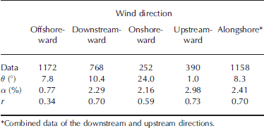
Since the wind directed offshore is affected by the local land breeze, we first examine the dependence of the drift characteristics on wind direction. the wind data are separated into four cases: the offshore-, downstream-, onshore- and upstreamward directions (Fig. 1). the offshoreward wind is defined as wind with its direction in a 90^˚ range, with the offshoreward direction (25^˚ clockwise from the north) at its center. the downstreamward (upstreamward) wind range has its center roughly in the east-southeast (west-northwest) direction.

The wind factor and correlation coefficient are quite different for the offshoreward wind case (Table 2). They are much smaller than for the other cases, indicating that the wind speed is stronger at the coast than at the mooring site and the relative ice velocity cannot be expressed well by the coastal wind. Also, the wind factor and correlation coefficient for the onshoreward wind case are smaller than for the downstream- and upstreamward wind cases. This suggests that the internal ice stress is more important for the case with the onshoreward wind which advects sea ice towards the coast, especially because the mooring sites were near the coast. For these reasons, we exclude the data with the across-shore wind from the following analyses and concentrate on the data with the alongshore wind, which is more reliable at the coast. (For the tables, however, we also retain the drift characteristics based on the wind data in all directions.)

Table 2. Sea-ice drift characteristics for different wind directions during 1999–2001

4.2. Dependence on wind speed

Equation (3) is derived from Equation (1) assuming the conditions with moderate to strong wind so that the Coriolis and pressure-gradient terms are comparably smaller than the wind and water stresses. As expected from this assumption, the correlation coefficient increases as the wind increases for wind speed more than 2 ms^–1 (Table 3), indicating that the relative ice velocity is better expressed by the wind. Note that the turning angle decreases and the wind factor increases as the wind speed increases as shown by the previous theoretical studies (Reference Gaskill, Lopez and SwatersGaskill and others, 1980; Reference Thorndike and ColonyThorndike and Colony, 1982; Pease and Reference Pease and OverlandOverland, 1984; Reference Leppäranta and LeppärantaLeppäranta, 1998, 2005). Since the correlation coefficient is <0.4 for the data with wind speed <2ms^–1, we exclude these data from the following analyses.

Table 3. Sea-ice drift characteristics for different ranges of wind speed during 1999–2001. Both values for the alongshore wind direction and all the wind directions (in parentheses) are listed

4.3. Dependence on sea-ice thickness

Since the simultaneous ice-thickness data are available from the IPS, we also examine the dependence of sea-ice drift characteristics on ice thickness. This analysis is not possible for other observational methods such as buoy- or satellite-based remote sensing and drifting ice station. the turning angle increases and the wind factor decreases as ice thickness increases for the ranges larger than 0.5 m (Table 4). This is because the Coriolis force becomes more important and ice–water drag increases as ice thickness increases. These tendencies agree with the results of the previous theoretical studies (Gaskill and others, 1980; Pease and Overland, 1984; Reference Leppäranta and LeppärantaLeppäranta, 1998, Reference Leppäranta2005).

Table 4. Sea-ice drift characteristics for different ranges of ice thickness during 1999–2001. Both values for the alongshore wind direction and all the wind directions (in parentheses) are listed. the data are limited for wind speed >2ms^–1

5. Discussions and Summary

The free-drift balance expressed by Equation (3) is most applicable for the case with strong wind and small ice thickness, so the wind factor of 2.68% (defined as α ₀) is calculated from the data with wind speed >6ms^–1 and thickness 0–0.5 m. (The turning angle and correlation coefficient are 9.1^˚ and 0.84, respectively.) Using the ratio of surface wind to geostrophic wind of 0.5–0.7 in near-neutral conditions over sea ice (Reference LeppärantaLeppäranta, 2005), the wind factor of 1.5% derived by Reference Kimura and WakatsuchiKimura and Wakatsuchi (2000) in the Sea of Okhotsk with geostrophic wind corresponds to 2.1–3.0% with surface wind. the value of 2.68% is also within the range (2.5–3.0%) obtained in the Baltic Sea with surface wind (Reference Leppäranta and OmstedtLeppäranta and Omstedt, 1990).

Since the drag coefficients between air and ice, and ice and water are important factors for transferring momentum among them and crucial parameters in numerical models, there have been many observational studies of these drag coefficients in various ice-covered oceans (e.g. Reference OverlandOverland, 1985; Reference Martinson and WamserMartinson and Wamser, 1990; Reference Guest and DavidsonGuest and Davidson, 1991). In the Sea of Okhotsk, however, there have been a few observational studies (e.g. Reference Shirasawa and AotaShirasawa and Aota, 1991; Reference Fujisaki, Yamaguchi, Takenobu, Futatsudera and MiyanagaFujisaki and others, 2009). Reference Fujisaki, Yamaguchi, Takenobu, Futatsudera and MiyanagaFujisaki and others (2009) measured the air–ice drag coefficient, C _a, from an icebreaker off Hokkaido and derived a value of 2.7–3.1×10^–3. As described in section 1, the evaluation of the wind factor is roughly equivalent to that of the ratio between the air and water drag coefficients, C _a/C _w. Thus, we can estimate the water drag coefficient, which is more difficult to measure, from combining our results and those of Reference Fujisaki, Yamaguchi, Takenobu, Futatsudera and MiyanagaFujisaki and others (2009). Using the wind factor α ₀ = 2.68% defined above, C _w is estimated to be 4.5–5.1×10^–3. These are larger values than that of 3.5×10^–3 in the Baltic Sea (Reference Leppäranta and OmstedtLeppäranta and Omstedt, 1990) and close to those of 5.0×10^–3 in the Beaufort Sea (Reference McPheeMcPhee, 1982) and 5.4×10^–3 in the Barrow Strait (Reference Shirasawa and IngramShirasawa and Ingram, 1991).

For thick ice and/or weak wind, we need to retain the Coriolis and pressure-gradient terms in Equation (1). Gaskill

and others (1980), and Pease and Reference Pease and OverlandOverland (1984) calculated the wind factor and turning angle for varying ice thickness and wind speed in their theoretical studies. Reference Leppäranta and LeppärantaLeppäranta (1998, Reference Leppäranta2005) derived the equations for the wind factor, α, and turning angle, θ, for this case. They are

(7)

(8)

Here R is a dimensionless quantity defined as , where ρ _i and h _i are ice density and thickness and f is the Coriolis parameter. Thus, R is a measure of the importance of the Coriolis and pressure-gradient terms and it increases as ice thickness increases and wind speed decreases. Since we assume that the surface wind and near-surface water velocity used in this study act on the ice surface and bottom, we set θ _a = θ _w = 0 in these equations. Figure 4 shows the wind factor and turning angle in this case with α ₀ = 2.68%. the curves in Figure 4 show that the wind factor decreases and the turning angle increases as R increases. Also plotted by circles are the wind factors and turning angles obtained from the present dataset. Their values are calculated from the part of the dataset with different combinations of wind-speed and ice-thickness ranges shown in Tables 3 and 4, respectively. Values of R are determined from these combinations along with C _a = 2.7×10^–3 after Reference Fujisaki, Yamaguchi, Takenobu, Futatsudera and MiyanagaFujisaki and others (2009). Although there are some outliers, these results generally follow the theoretical curves from Equations (7) and (8). the wind factor decreases and the turning angle increases as R increases. the smaller wind factors than the theoretical values may be due to the effect of internal ice stress. Although the range of R is somewhat limited mainly due to the absence of thick ice, our dataset is a rare example of the dependence of drift characteristics on the combination of ice thickness and wind speed, and their resulting agreement with the theory. This is because it is not possible to collect sea-ice drift data along with thickness data (of a variety of thickness) by other methods such as remote-sensing and drifting-station observations.

Fig. 4. Curves of (a) the wind factor, α, and (b) turning angle, θ, against R derived from Equations (7) and (8) when θ _a = θ _w=0. Circles are values obtained from the data for the cases with different combinations of wind-speed and ice-thickness ranges. the ranges are the same as those shown in Tables 3 and 4. Only values obtained when the correlation coefficient, r, is >0.6 are plotted. R is calculated using C _a = 2.7×10^–3 after Reference Fujisaki, Yamaguchi, Takenobu, Futatsudera and MiyanagaFujisaki and others (2009). Note that the R-axis is drawn in a logarithmic scale for clarity.

This study clearly shows the utility of the moored ADCP measurement for studying sea-ice drift. This method is especially effective if the moored measurement of ice draft is carried out simultaneously. Limitations of this study are the assumption of steady-state balance and the quality of the across-shore wind data. the assumption of steady-state balance for the hourly-mean ice drift over the mooring is a rather simplified approach. the validity of this assumption cannot be tested strictly based on the available dataset and this remains an issue. However, the fact that the wind factor and turning angle change consistently with the theory may provide another support for considering the steady-state balance. the use of the objectively analyzed wind data, which are presumably free of land–sea breeze, with high temporal and spatial resolutions such as the Grid Point Value data produced by the Japanese Meteorological Agency (only available since October 2003) would enable us to examine sea-ice drift for all the wind directions.