2.1. Eulerian–Lagrangian method

The EL simulations presented here are based on the volume-filtered (VF) formulation (Anderson & Jackson Reference Anderson and Jackson1967; Jackson Reference Jackson2000; Capecelatro & Desjardins Reference Capecelatro and Desjardins2013). In the EL formulation the fluid phase is treated in the Eulerian frame as a continuum, while the particle phase is treated in the Lagrangian frame, with discrete particles tracked individually.

The VF conservation equations govern the fluid (carrier) phase in the semi-dilute regime (low particle volume fraction) as

(2.1a)\begin{gather} \boldsymbol{\nabla} \boldsymbol{\cdot} \boldsymbol{u} =0, \end{gather}

(2.1b)\begin{gather}\rho_f \left(\frac{\partial \boldsymbol{u}}{\partial t}+\boldsymbol{u}\boldsymbol{\cdot}\boldsymbol{\nabla}\boldsymbol{u}\right) ={-}\boldsymbol{\nabla}p+\mu_f \nabla^2\boldsymbol{u}+\boldsymbol{F}_p, \end{gather}

where $\boldsymbol {u}$ is the VF fluid velocity, $p$ is the VF pressure, $\rho _f$ is the fluid density and $\mu _f$ is the fluid viscosity. The term $\boldsymbol {F}_p$ represents momentum exchange from particles (dispersed phase) to fluid. For a semi-dilute concentration of particles ($\phi _p \ll 1$), $\boldsymbol {F}_p$ can be expressed as

(2.2)\begin{equation} \boldsymbol{F}_p ={-}\phi_p \left. \boldsymbol{\nabla}\boldsymbol{\cdot} \boldsymbol{\tau}\right|_p+\rho_p \phi_p \frac{(\boldsymbol{v}- \boldsymbol{u}|_p)}{\tau_p}, \end{equation}

where $\rho _p$ is the particle density, $\phi _p$ represents the volume fraction of particles in the fluid medium, $\tau _p = \rho _p d_p^2/(18 \mu _f)$ is the relaxation time scale of the particle to the fluid acceleration and $d_p$ the particle diameter. The total fluid stress, denoted as $\boldsymbol {\tau }$, is determined from the combination of pressure and viscous stresses as $-p\boldsymbol {I} + \mu _f (\boldsymbol {\nabla } \boldsymbol {u}+\boldsymbol {\nabla }\boldsymbol {u}^{\textrm {T}})$, where $\boldsymbol {\nabla } \boldsymbol {u}$ represents the fluid velocity gradient, $\boldsymbol {I}$ is the identity matrix and $({\cdot })^{\textrm {T}}$ is the transpose operator. The Eulerian particle velocity, $\boldsymbol {v}$, is computed from Lagrangian particle velocities using (2.4). The notation $({\cdot }) |_p$ specifies fluid properties evaluated at the locations of the particles. The fluid velocity at the particle location ($\boldsymbol {u}|_p$) is obtained through a trilinear interpolation, as described in Capecelatro & Desjardins (Reference Capecelatro and Desjardins2013). In (2.2) the first term represents the stress exerted by the undisturbed flow at the location of the particle. The next term accounts for stresses induced by the presence of particles, characterized by Stokes drag, for $Re_p \ll 1$, where $Re_p$ is the Reynolds number based on particle size. The Stokes drag must be evaluated using the slip velocity between the particle and the undisturbed fluid. In situations where the density ratio ($\rho _p/\rho _f$) is significantly higher (e.g. dusty gas flows, water droplets in the air), as in our study, Stokes drag dominates the momentum exchange. Since the density ratio is very large and the particle volume fraction is very low, the first term in (2.2) is negligible compared with the second term. Although our EL simulation implementation generally accounts for both of these terms, we will later see in § 4 that, in the LSA, only the Stokes drag term is used, and the first term is neglected for simplicity.

The particles are tracked in a Lagrangian sense. Assuming point spherical particles in a $Re_p \ll 1$ flow regime, the dynamic equation for ${i}{\rm th}$ particle is given by Maxey & Riley (Reference Maxey and Riley1983) as

(2.3)\begin{equation} \frac{{\rm d}\boldsymbol{v}^i}{{\rm d} t} = \frac{1}{\rho_p} \left. \boldsymbol{\nabla} \boldsymbol{\cdot} \boldsymbol{\tau}\right|_p+\frac{\left. \boldsymbol{u}\right|_p-\boldsymbol{v}^i}{\tau_p},\quad \textrm{with} \ \frac{{\rm d}{\kern0.9pt}\boldsymbol{x}^i}{{\rm d}t} = \boldsymbol{v}^i, \end{equation}

where $\boldsymbol {x}^i$ and $\boldsymbol {v}^i$ are the position and velocity of the ${i}{\rm th}$ particle, respectively. In this study, gravitational/sedimentation effects have been omitted to isolate and comprehend the distinctive impact of two-way coupling on instability. Also, we operate in the semi-dilute regime to avoid any potential particle–particle interactions such as collision. Also, as mentioned earlier, the density ratio ($\rho _p/\rho _f$) is kept large, so the added mass effect, Basset history force and Saffman lift force are negligible. To evaluate the momentum feedback from the particle phase to the fluid phase ($\boldsymbol {F}_p$), one needs to evaluate the instantaneous particle volume fraction and Eulerian particle velocity field. At a location $\boldsymbol {r}$, these are obtained from the corresponding instantaneous Lagrangian quantities using

(2.4a)\begin{gather} \phi_p(\boldsymbol{r}) = \sum_{i = 1}^{N}V_p g(\lVert \boldsymbol{r}-\boldsymbol{x}^i\rVert), \end{gather}

(2.4b)\begin{gather}\phi_p(\boldsymbol{r}) \boldsymbol{v}(\boldsymbol{r}) = \sum_{i = 1}^{N}\boldsymbol{v}^iV_p g(\lVert \boldsymbol{r}-\boldsymbol{x}^i\rVert), \end{gather}

where $V_p = {\rm \pi}d_p^3/6$ is the particle volume, $g$ represents a Gaussian filter kernel of size $\delta _f = 3 \Delta x$, where $\Delta x$ is the grid spacing (Capecelatro & Desjardins Reference Capecelatro and Desjardins2013). In the VF method the Gaussian kernel smoothes out/regularizes the fluctuations in momentum feedback, thereby preventing any convergence issues during simulation. The VF model was recently applied by the authors successfully in particle-laden vortical flows (Shuai & Kasbaoui Reference Shuai and Kasbaoui2022; Shuai et al. Reference Shuai, Dhas, Roy and Kasbaoui2022, Reference Shuai, Roy and Kasbaoui2024). Readers interested in further details about the numerical approach may refer to them.

The Reynolds stress term, or the subgrid-scale tensor, is an important consideration during the filtering operation. In a multiphase flow like ours, this term can arise from (i) turbulent fluctuations in the fluid phase and (ii) fluctuations created by the particles. Since our simulations are not in the turbulent regime, the first contribution can be readily neglected. As for the contribution due to particle disturbances, it is not clear whether it is significant and how to model it. There are ongoing efforts to model the particle-induced subfilter-scale tensor, such as the recent work by Hausmann, Evrard & van Wachem (Reference Hausmann, Evrard and van Wachem2023). However, due to the large modelling uncertainty, there is no clear consensus on how to model these subfilter effects. These considerations are outside the scope of this paper, and thus, we neglect subfilter-scale effects other than those that appear in the feedback force in our analysis.

The works of Sundaram & Collins (Reference Sundaram and Collins1996) and Peskin (Reference Peskin2002) demonstrated that, in EL simulations, using different schemes for interpolating fluid velocity at particle positions and for extrapolating particle feedback forces to the fluid phase can result in an error gap in the kinetic energy budget. However, this issue pertains specifically to point-particle models, where discrete Dirac delta functions acting on the Navier–Stokes equations represent the particle feedback force. Our method, by contrast, follows a VF approach, as outlined by Capecelatro & Desjardins (Reference Capecelatro and Desjardins2013), where the governing equations are derived via convolution with a smooth kernel, such as a Gaussian. A comparison of both methods with experimental results for the case of a particle-laden vertical turbulent channel flow can be found in Wang et al. (Reference Wang, Fong, Coletti, Capecelatro and Richter2019). Given the fundamental differences in our approach, the kinetic energy gap highlighted by Sundaram & Collins (Reference Sundaram and Collins1996) does not apply to our simulations despite using trilinear interpolation for fluid velocity at particle positions and a Gaussian kernel for particle feedback. While we are unaware of any hidden energy imbalance, this falls beyond the scope of the present study. Furthermore, Ireland & Desjardins (Reference Ireland and Desjardins2017) demonstrated that applying additional corrections to the fluid velocity at particle positions did not lead to statistically significant variations in time-averaged quantities, such as fluctuation energy or fluid kinetic energy.

In (2.2) and (2.3), when evaluating the drag term, the fluid velocity at the particle location, $\boldsymbol {u}|_p$, should ideally represent the undisturbed flow. However, since the simulation accounts for the presence of particles, the fluid velocity is already disturbed, making it challenging to accurately estimate the undisturbed flow velocity. This error can lead to unphysical, self-induced particle motion, which is a known challenge in EL simulations. The self-induced motion is influenced by the length scale of the interpolation kernel $g$. Studies such as Ireland & Desjardins (Reference Ireland and Desjardins2017) and Balachandar, Liu & Lakhote (Reference Balachandar, Liu and Lakhote2019) have proposed corrections for estimating $\boldsymbol {u}|_p$, to reduce the risk of this unphysical phenomenon. These studies suggest that the correction for self-induced velocity is proportional to the ratio of particle diameter to filter width, $d_p/\delta _f$. To minimize the effect, one must maintain $d_p/\delta _f \ll 1$, ensuring that the kernel's length scale is large enough and that many particles lie within the volume occupied by the kernel. Consequently, the flow is modified by the collective effect of many particles, making the individual self-induced motion negligible.

A scaling analysis of the drag force in (2.2) reveals the coupling strength of feedback force from particle phase to fluid phase is governed by the non-dimensional number $M = \rho _p \langle \phi _p \rangle /\rho _f$ – the mass loading (or mass fraction), where $\langle \phi _p \rangle$ is the average volume fraction of particles. If the particle field is dilute and the mass loading is negligible, the feedback force can be neglected, and the one-way coupled simulations can be used to describe the evolution of the particulate flow. However, when the density ratio ($\rho _p/\rho _f$) is significant, as is the case here, the mass loading becomes ${O}(1)$, which leads to significant feedback to the fluid phase from the particle phase, even if the particle phase is dilute (Kasbaoui et al. Reference Kasbaoui, Koch, Subramanian and Desjardins2015). As we will see in the upcoming sections, this feedback is the source of instability in the present study, as the system considered here is stable under one-way coupling.

2.2. Illustration of the instability

To demonstrate the instability resulting from two-way coupling, we investigate an unbounded simple shear flow combined with a band of particles distributed in a top-hat manner (refer to the schematic in figure 1). The fluid properties include a density of $\rho _f = 1.0 \ \textrm {Kg}\ \textrm {m}^{-3}$, viscosity of $\mu _f = 1.5\times 10^{-5}\ \textrm {Kg}\ \textrm {m}^{-1}\ \textrm {s}^{-1}$ and a flow shear rate of $\varGamma = 12.65\ \textrm {s}^{-1}$. The particles are monodisperse with a diameter $d_p = 4.62 \ \mathrm {\mu } \textrm {m}$ and density $\rho _p = 1000\ \textrm {Kg}\ \textrm {m}^{-3}$, distributed uniformly within a region $\lvert y \rvert \leqslant h/2$. The band width is chosen as $h = 6\ \textrm {mm}$ to maintain a large $h/d_p$ ratio, approximately $h/d_p \approx 1300$, ensuring that the fluctuations caused by discrete particle forcing remain well below the viscous dissipation scale. The average volume fraction of particles within the band is set to $\langle \phi _p \rangle = 10^{-3}$. In terms of non-dimensional numbers, this corresponds to a density ratio of $\rho _p/\rho _f = 1000$, Stokes number $St =\varGamma \tau _p= 10^{-3}$ and mass loading $M = (\rho _p/\rho _f) \langle \phi _p \rangle = 1$, which is significant. Here, $\tau _p = \rho _p d_p^2/(18 \mu _f)$ is the particle relaxation time.

The relative importance of the gravitational settling speed ($V_s = g \tau _p$) of particles compared with the characteristic flow speed ($V_c = \varGamma h$) can be evaluated as $V_s/V_c = St/Fr^2 \approx 0.01$. Here, $g$ is the acceleration due to gravity and $Fr = V_c/\sqrt {g h}$ is the Froude number, a dimensionless number that measures the relative importance of inertial forces to gravitational forces. Given that the ratio $V_s/V_c$ is very small, it is evident that the gravitational settling effect of particles is negligible in this set-up. Consequently, we have ignored it in our study. Furthermore, the Saffman lift force (Saffman Reference Saffman1965) experienced by a particle moving in a simple shear flow is given by $\boldsymbol {L} = 1.615 \mu _f d_p \lvert \boldsymbol {u}_s\rvert \, \sqrt {d_p^2 \lvert \boldsymbol {\omega }\rvert \rho _f/\mu _f}\, (\boldsymbol {\omega } \times \boldsymbol {u}_s)/(\lvert \boldsymbol {\omega }\rvert \, \lvert \boldsymbol {u}_s\rvert )$ (see Candelier et al. (Reference Candelier, Mehaddi, Mehlig and Magnaudet2023) for a generalization of inertial forces in linear flows, accounting for transient effects). When compared with the Stokes drag $\boldsymbol {D} = 3 {\rm \pi}\mu _f d_p \boldsymbol {u}_s$, this yields $\lvert \boldsymbol {L}\rvert /\lvert \boldsymbol {D}\rvert \sim (1.615/{\rm \pi} )\, \sqrt {2 \,St\, \rho _f/\rho _p} \simeq 7.27 \times 10^{-4}$. Here, $\boldsymbol {u}_s$ is the slip velocity between the particle and the fluid, and $\boldsymbol {\omega }$ is the vorticity at the particle location, assumed to scale with the background shear rate as $\lvert \boldsymbol {\omega }\rvert \sim \varGamma$. The negligible ratio of lift to drag force allows us to ignore the lift force in this study, as reflected in (2.3).

The numerical simulation is performed in a box of dimensions $L_x\times L_y\times L_z$, where $L_x \approx 16\,666 d_p$, $L_y = 3 L_x$ and $L_z = 3 d_p$. To avoid unwanted diffusion effects, the Reynolds number based on the box width is thus set to $Re_{L_x} = \varGamma L_x^2\rho _f/\mu _f \approx 5000$, and we focus on inviscid instability. The flow needs to be periodic in the $x$ direction and unbounded in the $y$ direction. To achieve this within the simulation box, we apply regular periodic boundary conditions at the left and right boundaries (in the $x$ direction) and shear-periodic boundary conditions at the top and bottom boundaries (in the $y$ direction), accounting for the background shear flow (see Kasbaoui et al. Reference Kasbaoui, Patel, Koch and Desjardins2017). By choosing a domain size that is three times larger in the $y$ direction, we ensure neighbouring periodic simulation boxes are well separated and do not interfere with each other to influence the instability. We use the EL framework described above on a uniform Cartesian grid with resolution $h/\Delta x \approx 41$, $N_x = 512$, $N_y = 3 N_x$ and $N_z = 1$. The ratio $d_p/\delta _f$ is maintained at approximately $0.01$, a sufficiently small value, ensuring that the self-induced motion of particles is negligible. Here, we perform pseudo-two-dimensional simulations by considering only one grid point in the axial ($z$) direction with periodic boundary conditions applied over a thickness $\Delta z = 3 d_p$. This allows the definition of volumetric quantities such as particle volume and volume fraction.

In addition to conducting two-way coupled simulations, we perform one-way coupled simulations, where the momentum exchange term (2.2) is neglected. The particles still evolve due to the momentum contribution from the fluid. However, the particles’ feedback to the fluid phase is deliberately switched off. This allows for comparison between one-way and two-way coupled simulations and showcases the impact of particle feedback on the flow dynamics.

The fluid velocity field is initially superimposed with a two-dimensional incompressible perturbation of the form $\tilde {u}_x = \epsilon \varGamma h\,{\rm e}^{-y^2/\beta ^2}\, (2y/k \beta ^2)\sin k x$ and $\tilde {u}_y = \epsilon \varGamma h\, {\rm e}^{-y^2/\beta ^2} \cos k x$. The perturbation has an amplitude of $\epsilon = 10^{-2}$ relative to the characteristic flow velocity $\varGamma h$, where, as mentioned earlier, $\varGamma = 12.65\ \textrm {s}^{-1}$ and $h = 6\ \textrm {mm}$. It features a sinusoidal variation in the $x$ direction, set to contain four full periods in the domain, i.e. $\lambda = L_x/4$, where $\lambda$ is the wavelength of the perturbation in the $x$ direction (i.e. $k h = 2$ with dimensional wave number $k = 2{\rm \pi} /\lambda$). The perturbation decays in the $y$ direction in a Gaussian manner with a characteristic width $\beta = 2 h$. The corresponding perturbation vorticity field is shown in figure 2, at $\varGamma t = 0$. The initial velocity of the particles is set equal to the local fluid velocity.

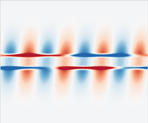
Figure 2. The time evolution of isocontours of normalized perturbation vorticity ($\tilde {q}_z/\tilde {q}_0$) for two-way coupling (a–e) and one-way coupling (f–j) is shown. The corresponding simulation parameters are set to $M=1$, $St = 10^{-3}$, $\epsilon = 10^{-2}$ and $\langle \phi _p \rangle = 10^{-3}$. For better visualization, the figures are zoomed in and cropped to centre the view on the particle band, although the simulation domain is larger, especially in the $y$ direction. In addition, the coordinates in both directions are scaled with the band width $h$.

The evolution of the vorticity perturbation $\tilde {q}_z$ normalized by its initial maximum value $\tilde {q}_0 = \epsilon \varGamma h\, (k+2/(k \beta ^2)) = (9/4) \epsilon \varGamma$ is presented in figure 2. Successive snapshots are provided for various non-dimensional times $\varGamma t = 0, 0.1, 1, 2$ and $3$. The snapshots are confined to a domain that is zoomed in and cropped around the particle band for better visualization, although the simulations use a larger domain size, especially in the $y$ direction, as mentioned earlier. In the case of one-way coupling (f–j), it is observed that the vorticity patches are sheared, tilted and stretched by the background flow, and the intensity of vorticity diminishes as time progresses. The downstream tilt of the vorticity perturbations and the related algebraic decay of associated perturbation energy by the Orr mechanism are described in detail in Farrell (Reference Farrell1987) and Roy & Subramanian (Reference Roy and Subramanian2014). The perturbed flow had a periodic behaviour with a wavelength in the $x$ direction of $\lambda = L_x/4$, which remains unchanged as time advances. At later times, it can be seen that the perturbation field eventually decays.

Conversely, when considering two-way coupling (a–e), we observe significant evolution and amplification of the vorticity field. The initially perturbed mode with $\lambda = L_x/4$ disappears, giving way to a new mode with $\lambda = L_x$. These newly emerged structures, likely unstable eigenmodes, persist and their corresponding vorticity field intensifies over time. As the simulation progresses, nonlinear interactions between successive vorticity patches become more pronounced, eventually leading to a transition into a strongly nonlinear regime (not shown here).

Particle dispersion is also significantly affected when two-way coupling is considered. Figure 3 depicts the evolution of the particle volume fraction field scaled with the average initial volume fraction. When the particle feedback is neglected (f–j), the shear flow simply advects the particles. As the flow perturbations decay over time, they have minimal impact on particle transport, even after a significantly longer duration. Eventually, the disturbances die out and the particle distribution resembles the initial band (see figure 3(f–j) at $\varGamma t = 0$ and $25$). In contrast, two-way coupling leads to growing flow perturbations, which in turn govern the dispersion of particles (a–e). Initially, the uniform particle band undergoes deformation due to flow disturbances characterized by a periodic mode of $\lambda = L_x$. As time progresses, the interplay between background shear flow and growing perturbations initiates nonlinear effects, resulting in particle clustering into lobes interconnected by a relatively slender filament, as can be seen in figure 3(a–e), at $\varGamma t=25$.

Figure 3. The time evolution of isocontours of the normalized particle number density ($n = \phi _p/\langle \phi _p \rangle$), corresponding to the simulation in figure 2, is shown. The large time snapshots illustrate the nonlinear evolution of the instability in the two-way coupling case.

The simulations shown in figures 2 and 3 suggest that semi-dilute inertial particles, distributed non-uniformly in an unbounded simple shear flow, can induce hydrodynamic instability. This instability cannot be solely attributed to hydrodynamics since the simple shear flow in a single-phase flow is stable to infinitesimal perturbations (see Drazin & Reid Reference Drazin and Reid2004). Furthermore, it cannot be attributed to collisional effects, as the simulation neglected particle–particle interactions. Instead, the instability must arise from the two-way momentum exchange between the two phases, as confirmed by the absence of instability when the two-way coupling term is deactivated in the simulation. Previous studies have shown that uniformly distributed particles in a simple shear flow, even with two-way coupling, do not exhibit modal instability but can demonstrate only a non-modal instability if gravitational effects are considered (Kasbaoui et al. Reference Kasbaoui, Koch, Subramanian and Desjardins2015). However, in this study we observe the emergence of a new type of instability resulting from the interaction between the simple shear flow and a non-uniformly distributed particle field in the absence of gravitational settling. In the subsequent sections we demonstrate that this new type of instability is modal and explain its generation mechanism. The following section will provide a mechanistic explanation of the instability through wave interactions.

4.1. Two-fluid model

We adopt the Eulerian–Eulerian description of a particle-laden flow, as outlined by previous works such as Saffman (Reference Saffman1962); Marble (Reference Marble1970); Druzhinin (Reference Druzhinin1995); Jackson (Reference Jackson2000); Kasbaoui et al. (Reference Kasbaoui, Koch, Subramanian and Desjardins2015). The dispersed phase, or particle phase, is characterized by a set of conservation equations inspired from the kinetic theory of gases, employing a mono-kinetic particle velocity distribution function. According to the method, the particle phase is considered a continuum fluid of zero pressure, valid for very dilute suspensions. The mass and momentum conservation equations for the fluid and particle phases in the semi-dilute regime, expressed in non-dimensional form, are

(4.1a)\begin{gather} \boldsymbol{\nabla} \boldsymbol{\cdot} \boldsymbol{u} =0, \end{gather}

(4.1b)\begin{gather}\frac{\partial n}{\partial t}+\boldsymbol{\nabla}\boldsymbol{\cdot}(n\boldsymbol{v}) = 0, \end{gather}

(4.1c)\begin{gather}\frac{\partial \boldsymbol{u}}{\partial t}+\boldsymbol{u}\boldsymbol{\cdot}\boldsymbol{\nabla}\boldsymbol{u} ={-}\boldsymbol{\nabla}p+\frac{1}{Re} \nabla^2\boldsymbol{u}+M \frac{ n (\boldsymbol{v}-\boldsymbol{u})}{St}, \end{gather}

(4.1d)\begin{gather}\frac{\partial (n\boldsymbol{v})}{\partial t}+\boldsymbol{\nabla} \boldsymbol{\cdot} \left(n \boldsymbol{v}\boldsymbol{v}\right) = \frac{n (\boldsymbol{u}-\boldsymbol{v})}{St}, \end{gather}

where, as mentioned earlier, $\boldsymbol {u}$ represents the fluid velocity, $\boldsymbol {v}$ denotes the particle velocity and $n = \phi _p/\langle \phi _p \rangle$ is the normalized particle number density; but all depicted as fields here. Here onwards, we drop $()^*$ from non-dimensional quantities as we only deal with them unless specified otherwise. For non-dimensionalization, the length and time scales are set to the initial width of the particle band ($h$) and the inverse shear rate ($\varGamma ^{-1}$), respectively. The dimensional number density $\phi _p/V_p$ is normalized by $\langle \phi _p \rangle /V_p$ to obtain a non-dimensional measure for the particle concentration field denoted as $n = \phi _p /\langle \phi _p \rangle$, where $V_p$ represents the particle volume. The non-dimensional numbers include the Reynolds number ($Re=\varGamma h^2/\nu$), which quantifies fluid inertia, the Stokes number ($St = \varGamma \tau _p$), characterizing particle inertia, and, as mentioned earlier, the particle mass loading $M = \rho _p \langle \phi _p \rangle / \rho _f$. We have not accounted for particle interactions and inertial lift forces in our current formulation, although these effects could alter particle trajectories significantly. Both hydrodynamic and non-hydrodynamic interactions among dust particles can influence particle trajectories, affecting phenomena like coagulation and deposition (see Patra, Koch & Roy (Reference Patra, Koch and Roy2022) and references therein). In this study we focus on the highly dilute limit and neglect the role of any interactions. The non-zero slip velocity a particle has with its background local shear flow causes it to experience an inertial lift force, as derived by Saffman (Reference Saffman1965) for a simple shear flow scenario. The magnitude of the Saffman lift force depends on the particle Reynolds number based on the local shear rate. In our problem this Reynolds number is small; hence, we disregard the effect of inertial lift.

4.1.1. Linearization and normal mode analysis of the inviscid equations

We disregard viscous effects in the analytical approach and focus solely on the inviscid scenario, where $Re \rightarrow \infty$, as we have seen that the mechanism of the instability is inherently inviscid. For stability analysis, we linearize the governing equations (4.1). The flow quantities are split into their base state, denoted by capital letters, and perturbation, denoted with a tilde, such as $\boldsymbol {u} = \boldsymbol {U}+\tilde {\boldsymbol {u}}$, $\boldsymbol {v} = \boldsymbol {V}+\tilde {\boldsymbol {v}}$, $p = P+\tilde {p}$ and $n = N+\tilde {n}$. We consider a two-dimensional stability analysis in the $x$–$y$ plane. A general base state of the form $\boldsymbol {U} =\boldsymbol {V}= U(y) \hat {\boldsymbol {x}}$ and $N = N(y)$ satisfies the governing equations (4.1). That is, it is assumed that there is no slip between the base state particle and fluid velocities. Perturbing the base state with two-dimensional infinitesimal disturbances of the form $\tilde {\boldsymbol {u}}(x,y,t)$, $\tilde {\boldsymbol {v}}(x,y,t)$, $\tilde {p}(x,y,t)$ and $\tilde {n}(x,y,t)$, we obtain the linearized version of the equations as

(4.2a)\begin{gather} \boldsymbol{\nabla} \boldsymbol{\cdot} \tilde{\boldsymbol{u}} = 0, \end{gather}

(4.2b)\begin{gather}\frac{\partial \tilde{n}}{\partial t} + U \frac{\partial \tilde{n}}{\partial x} + \tilde{v}_y \frac{{\rm d}N}{{\rm d}y} +N \boldsymbol{\nabla} \boldsymbol{\cdot} \tilde{\boldsymbol{v}} = 0, \end{gather}

(4.2c)\begin{gather}\frac{\partial \tilde{\boldsymbol{u}}}{\partial t} + U \frac{\partial \tilde{\boldsymbol{u}}}{\partial x} + \tilde{u}_y \frac{{\rm d} U}{{\rm d}y} \hat{\boldsymbol{x}} ={-}\boldsymbol{\nabla} \tilde{p}+M \frac{ N (\tilde{\boldsymbol{v}}-\tilde{\boldsymbol{u}})}{St}, \end{gather}

(4.2d)\begin{gather}\frac{\partial (N \tilde{\boldsymbol{v}})}{\partial t} + U \frac{\partial (N\tilde{\boldsymbol{v}})}{\partial x} + N \tilde{v}_y \frac{{\rm d}U}{{\rm d}y} \hat{\boldsymbol{x}} = \frac{ N(\tilde{\boldsymbol{u}}-\tilde{\boldsymbol{v}})}{St}. \end{gather}

Here $\tilde {\boldsymbol {u}} = \tilde {u}_x \hat {\boldsymbol {x}}+\tilde {u}_y \hat {\boldsymbol {y}}$ and $\tilde {\boldsymbol {v}} = \tilde {v}_x \hat {\boldsymbol {x}}+\tilde {v}_y \hat {\boldsymbol {y}}$, where $\hat {\boldsymbol {x}}$ and $\hat {\boldsymbol {y}}$ are the unit vectors in the $x$ and $y$ direction, respectively. While it may appear that $N$ could be scaled out of all the terms in (4.2d), it is retained because one must consider that in regions where there are no particles, $N = 0$, $\tilde {\boldsymbol {v}} = (N\tilde {\boldsymbol {v}})/ N$ cannot be defined in these empty regions. We use two-dimensional disturbances, following Squire's theorem (Squire Reference Squire1933), according to which the most unstable modes should be two dimensional, which is valid for dusty flows as well (Sozza et al. Reference Sozza, Cencini, Musacchio and Boffetta2022). To solve the system, we utilize a standard approach of normal mode analysis. Since the linearized equations (4.2) are homogeneous in $x$ and $t$, we assume a normal mode form for the solutions as $\{\tilde {\boldsymbol {u}},\tilde {\boldsymbol {v}},\tilde {p},\tilde {n}\} = \{\hat {\boldsymbol {u}},\hat {\boldsymbol {v}}, \hat {p}, \hat {n}\}(y)\exp ({{\rm i}(k x-\omega t)})$, to obtain the eigenvalue system, similar to the one in Saffman (Reference Saffman1962) (see Appendix A). Here $k$ is the non-dimensional wavenumber in the $x$ direction (scaled by $h$) and $\omega$ is the non-dimensional angular frequency (scaled by $\varGamma$). The complex wave speed is defined as $c = c_R+{\rm i} c_I = \omega /k$. For temporal stability analysis (real valued $k$), the real part ${\rm Re}(c)=c_R$ determines the phase speed of the wave propagation and the imaginary part ${\rm Im}(\omega ) = c_I k = \sigma$ determines the growth rate. If ${\rm Im}(\omega )<0$, the mode is stable, while if ${\rm Im}(\omega )>0$, it is unstable. We need to solve the linear eigenvalue system equations (A2), seeking the eigenvalues $c$ (or $\omega$) and eigenfunctions $\{\hat {u}_x, \hat {u}_y, \hat {p},\hat {v}_x, \hat {v}_y, \hat {n}\}$, where $\hat {\boldsymbol {u}}= \hat {u}_x \hat {\boldsymbol {x}}+ \hat {u}_y \hat {\boldsymbol {y}}$ and $\hat {\boldsymbol {v}}= \hat {v}_x \hat {\boldsymbol {x}}+ \hat {v}_y \hat {\boldsymbol {y}}$.

Note that the particle velocity disturbance field influences the evolution of perturbation number density, although there is no feedback from number density perturbations to other quantities. To simplify the analysis, (4.2a,c,d) can be combined to obtain a single equation by eliminating variables $\tilde {u}_x$, $\tilde {p}$, $\tilde {v}_x$ and $\tilde {v}_y$. Following the approach outlined by Saffman (Reference Saffman1962), Asmolov & Manuilovich (Reference Asmolov and Manuilovich1998), this can be achieved in the modal space to obtain a simplified nonlinear eigenvalue system involving only two variables $\hat {u}_y$ and $\hat {n}$ as

(4.3a)\begin{gather} \big[\mathcal{U} (D^2-k^2)-\mathcal{U}''\big]\hat{u}_y+M D\big[(U-c) \varLambda N' \hat{u}_y\big] = 0, \end{gather}

(4.3b)\begin{gather}{\rm i}k (U-c)\varLambda \hat{n}+D[N \varLambda^2] \hat{u}_y=0, \end{gather}

where $\mathcal {U}= (U-c)(1+ M N \varLambda )$ denotes a modified base state velocity, and the damping factor $\varLambda = (1+{\rm i}k \, St (U-c))^{-1}$ describes the averaged frequency response of the particle phase to fluctuations in fluid velocity. We use $D({\cdot })$ or $({\cdot })'$ to represent the differential operator ${{\rm d}}{{\rm d}y}$, where generally the former one is reserved for perturbation quantities and the latter one reserved for base state quantities. Equation (4.3a) represents a modified form of the Rayleigh equation in the context of instability of dusty rectilinear flows, which we will now refer to as the ‘dusty Rayleigh equation’ or DRE for short. Note that the compact form of (4.3a) may misdirect the reader that the curvature of the number density field (i.e. $N''$) plays a role in the instability. However, the terms containing $N''$ exactly cancel out and do not have any role, which will be apparent from the form given in (A4a). A derivation of (4.3) can be found in Appendix A. These equations differ from those in Saffman (Reference Saffman1962) in that the latter considers a uniform base state number density field, leading to the absence of terms containing gradients of particle concentration. Additionally, they consider a viscous case with finite Reynolds number effects. However, we consider an inviscid scenario and non-uniform particle distribution, resulting in DRE (4.3a) instead of the modified Orr–Sommerfeld equation obtained by Saffman (Reference Saffman1962).

4.2. Linear stability analysis for inertialess ($St = 0$) particles and the dusty Rayleigh criterion

In this section we show that the instability is present even in the vanishing particle inertia limit, so the origin of the instability is attributed to the mass loading, which quantifies the two-way coupling. In the inertialess limit, i.e. $St = 0$, the damping factor is $\varLambda = 1$ and the modified velocity becomes a linear mapping of the actual base flow as $\mathcal {U} = (U-c)(1+ M N)$. Thus, (4.3) can be reduced to

(4.4a)\begin{gather} \rho\big[(U-c) (D^2-k^2)-U''\big]\hat{u}_y+\rho' \big[(U-c) D-U'\big]\hat{u}_y = 0, \end{gather}

(4.4b)\begin{gather}{\rm i}k (U-c) \hat{n}+ N' \hat{u}_y = 0, \end{gather}

where we denote $\rho := 1+M N$. The term $\rho$ is the equivalent of a variable density, where its variation contributes to the inertial term, leading to the generation of non-Boussinesq baroclinic vorticity. Moreover, the same (4.4) can also be derived from linearization and normal mode analysis of the single-fluid model (see Ferry & Balachandar Reference Ferry and Balachandar2001; Rani & Balachandar Reference Rani and Balachandar2003), as in the limit of $St \rightarrow 0$, the two-fluid model reduces to a stratified incompressible fluid system as we have seen in § 3.

The dusty Rayleigh criterion: the classic Rayleigh equation results in a necessary criterion for instability known as the inflection point theorem, which states that the base state velocity profile should exhibit an inflection point within the domain, meaning that the quantity $U''$ should change sign somewhere within the flow domain. The equivalent criterion in the context of (4.4a) is that the quantity $\varSigma = D[\rho U']$ should change sign within the flow domain. We have already seen the same term $\varSigma$ in (3.6), which generates vorticity disturbances and, thus, instability. A derivation of the modified Rayleigh criterion/dusty Rayleigh criterion can be found in Appendix B. An equivalent statement for piecewise linear base state profiles is that the two interfaces must exhibit opposite-signed jumps in $(\rho U')$ across them.

We investigate the stability of a particle-laden simple shear flow, corresponding to the EL simulation in § 2.2, where an unbounded simple shear flow interacts with particles localized within a band, as illustrated in figure 1. The respective non-dimensional form of the linear base state velocity profile is $U = y$ and the piecewise constant top-hat number density profile is

(4.5)\begin{equation} N(y) = \begin{cases} 1, & \textrm{if } -\frac{1}{2} \leqslant y \leqslant \frac{1}{2}, \\ 0, & \textrm{otherwise}, \end{cases} \end{equation}

where, as mentioned earlier, the inverse shear rate ($\varGamma ^{-1}$) is used as the time scale and the width of the band ($h$) is used as the length scale. In our case of a simple shear flow, the DRE stated above simplifies to a sign change for $N'$ in the flow domain, i.e. the gradient of the base state number density profile must exhibit a sign reversal for instability. In another sense, for the piecewise profile in (4.5), the instability criterion requires opposite-signed jumps in $\rho U'$ (or $N$ here) at the interfaces $y = \pm 1/2$, which is satisfied here. While the number density profile $N(y)$ defined in (4.5) is discontinuous, its form supports sharp gradients at the locations $y = \pm 1/2$, across which the sign flip occurs. It may be easier to visualize this sign flip if we smooth the number density profile, as we will see in (4.9) and figure 7. Overall, the base state meets the essential conditions for instability. However, instability is only assured once explicitly proven, as the dusty Rayleigh criterion serves as a necessary condition rather than a sufficient one. This section aims to analytically establish the presence of instability and pinpoint the parameter ranges where it manifests.

For the linear velocity profile and top-hat number density profile, the stability equations (4.4a) reduce to $(D^2-k^2)\hat {u}_y = 0$ for all $y$ values except at the two locations where the number density profile has a discontinuity, i.e. at the interfaces $y = \pm 1/2$. The solution to this equation can be obtained analytically and is expressed piecewise for each layer as

(4.6)\begin{equation} \hat{u}_y = \begin{cases} A_1 {\rm e}^{{-}k y}, & y > 1/2, \\ A_3 {\rm e}^{k y}+A_4 {\rm e}^{{-}k y}, & \lvert y \rvert < 1/2, \\ A_2 {\rm e}^{k y}, & y <{-}1/2, \end{cases} \end{equation}

where the unknown constants $A_1$ to $A_4$ need to be obtained from appropriate boundary conditions. Note that the decaying boundary condition for $\hat {u}_y$ at far field is already accounted for in the solution, i.e. $\hat {u}_y(y \rightarrow \pm \infty ) = 0$, assuming $k>0$. The kinematic criterion requires the continuity of $\hat {u}_y$ across the interfaces, ensuring the continuity of interface displacements ($\hat {\eta }$), as they are related through ${\rm i}k (U-c) \hat {\eta } = \hat {u}_y$. Additionally, integrating (4.4a) across the discontinuous interfaces provides corresponding dynamic conditions. For a detailed derivation, see Appendix C. Together, these conditions yield a system of four equations involving the unknowns $A_1$ to $A_4$ and $c$, as

(4.7)\begin{equation} \begin{bmatrix} 1 & 0 & - {\rm e}^{k} & - 1 \\ 0 & 1 & -1 & -{\rm e}^{k} \\ \alpha_1 & 0 & \alpha_2{\rm e}^{k} & -\alpha_2 \\ 0 & \alpha_3 & -\alpha_4 & \alpha_4{\rm e}^{k} \end{bmatrix}\begin{bmatrix} A_1 \\ A_2 \\ A_3 \\ A_4 \end{bmatrix}= \begin{bmatrix} 0 \\ 0 \\ 0 \\ 0 \end{bmatrix}, \end{equation}

where $\alpha _1 = k(1/2-c)-M$, $\alpha _2 = k(1/2-c)(1+M)$, $\alpha _3=k(1/2+c)-M$ and $\alpha _4 = k(1/2+c)(1+M)$. For a non-trivial solution to the system of (4.7), the determinant of the coefficient matrix must be zero, leading to the dispersion relation

(4.8)\begin{equation} c ={\pm} \frac{1}{2k}\sqrt{\frac{(k-2\,At)^2-At^2(2+k)^2{\rm e}^{{-}2k}}{1-At^2{\rm e}^{{-}2k}}}, \end{equation}

where the Atwood number ($At=(\rho _{max}-\rho _{min})/(\rho _{max}+\rho _{min})$) is related to the mass loading as $At = M/(M+2)$. Note that the eigenvalues $c$ appear in pairs, especially when ${\rm Im}(c) \neq 0$, they manifest as complex conjugates. Therefore, for instability to occur, ${\rm Im}(c)$ should not be zero. Equation (4.8) indicates the presence of a cutoff wavenumber ($k_{cutoff}$), below which only the instability can occur, i.e. long-wave instabilities. This critical wavenumber can be determined as the solution of the transcendental equation $M (2-k + (2+k){\rm e}^{- k})-2 k=0$. The variation of $k_{cutoff}$ with $At$ is shown in the figure 5(a). For instance, for a mass loading of $M=1 \ (\textrm {or}\ At=1/3)$, the critical wavenumber can be obtained as $k_{cutoff} \approx 1.028$. The resulting unstable modes are stationary since the corresponding ${\rm Re}(c) = 0$. Conversely, the modes are neutrally stable propagating waves for shorter wavelengths, i.e. when $k > k_{cutoff}$. In the limit of small $k$ values, instability is always present but with a lower growth rate, as evidenced by the scaling $\omega \sim \pm {\rm i} \,\sqrt {k}\, \sqrt {At/(1+At)}$.

Figure 5. (a) The variation of the cutoff wavenumber $k_{cutoff}$, at which the instability disappears, and the optimum wavenumber $k_{max}$, at which the maximum growth occurs, are plotted against the Atwood number for a top-hat number density profile. (b) The variation of the maximum growth rate $\sigma _{max}$, corresponding to $k_{max}$, with $At$ is shown for the same number density profile.

Upon substituting the solution for $c$ in (4.8) back into (4.7), the amplitudes $A_1$ to $A_4$ can be determined, as detailed in Appendix C. The dispersion relation (4.8) is plotted in figure 6, using continuous lines, for two different mass loading values. It can be observed from figure 6(a) that, for $k < k_{cutoff}$, the growth rate of the modes increases until reaching a maximum and then decreases for any given mass loading. Consequently, an optimal wavenumber ($k_{max}$) exists at which the maximum growth ($\sigma _{max}$) occurs. This optimal wavenumber can be obtained by solving the transcendental equation ${\rm e}^{2 k} (k-2\,At)+2\,At^2 (1+2\, At)\,(1-At+ k)+{\rm e}^{-2 k}\,At^4 (2+k) = 0$, derived from (4.8) using the optimization criteria ${\rm d} (c k)/{\rm d} k = 0$. Figure 5(a) displays the variation of $k_{max}$ with $At$ while figure 5(b) shows the variation of $\sigma _{max}$ with $At$. For instance, for $M=1 (\textrm {or}\ At=1/3)$, the non-dimensional wavenumber corresponding to the maximum growth rate is $k_{max} \approx 0.504$ and the maximum growth rate is $\sigma _{max} = k_{max}\, {\rm Im}(c(k_{max})) \approx 0.244$.

Figure 6. Dispersion relation for the $St = 0$ case, for two different mass loadings ($M=1$ – orange and $M=2$ – blue), obtained analytically (for a top-hat number density profile) and numerically (for two different smooth number density profiles: $m=1$ and $m=4$): (a) growth rate $\sigma$ (imaginary part of $\omega$) vs $k$, (b) real part of $\omega$ vs $k$.

From figure 6(b), it is evident that for $k > k_{cutoff}$, the waves propagate in opposite directions and attain a speed of $\omega \sim \pm (k/2 - At)$ as $k \rightarrow \infty$ (shown as asymptotes in the figure for $M=1$ in grey). This implies that the waves propagate without any interaction, as they are well separated by the distinct interfaces on which they exist. As we discussed the instability mechanism in § 3, we obtained the same dispersion relation earlier for isolated waves at the interface. The natural phase speed matching of the isolated left and right propagating waves occurs at $k = 2\, At$, as indicated by the crossing of these asymptotic lines in the dispersion curve. However, in practice, this matching occurs at $k_{cutoff} > 2\, At$ due to their interaction, as seen from the figure.

For the linear velocity profile and the top-hat number density profile, (4.4b) simplifies to $(y-c) \hat {n}=0$ everywhere except at the interfaces $y=\pm 1/2$. For the discrete modes (which corresponds to $y \neq c$), this equation yields $\hat {n} = 0$ everywhere except at the interfaces. Considering the interface discontinuity and conservation of the total number of particles, one finds that $\int _{-\infty }^{\infty } \hat {n}\, {{\rm d}y} = 0$, which implies that $\hat {n} \propto \delta (y-1/2)-\delta (y+1/2)$.

To verify the analytical results, we numerically solved the linear eigenvalue differential equation (4.4a) using a standard Chebyshev spectral collocation method. To avoid issues arising from the discontinuity of the base state number density profile, we employed a smooth generalized Gaussian profile for the number density:

(4.9)\begin{equation} N(y) = \exp \left\{-\left(\frac{y}{y^*}\right)^{2 m} \right\}, \quad \textrm{with} \ m \in \mathbb{N}. \end{equation}

Here $y^* = ( 2 \varGamma (1+1/(2 m) ) )^{-1}$, ensuring that the normalization yields $\int _{-\infty }^{\infty }N(y)\, {{\rm d}y} = 1$; $\varGamma ({\cdot })$ denotes the gamma function and $m$ is the smoothness parameter. The number density profile exhibits maximum smoothness for small integer values of $m$, whereas for larger values of $m$, it develops sharp variations. As $m$ tends to infinity, the profile approaches the singular top-hat profile described in (4.5), as ensured by the normalization. The plots in figure 7 depict the variation of the smooth base state number density profile and the corresponding stability-determining quantity $\varSigma$ for various smoothness parameters $m$ within the flow domain. The Chebyshev collocation points ranging from $y \in [-1,1]$ are transformed to $y \in [-R,R]$, where $R$ is chosen to be sufficiently large to mimic infinity. To enhance the efficiency of the numerical method by capturing the sharp variations near the interfaces more effectively, we use the transformation as in Govindarajan (Reference Govindarajan2004), which ensures that more collocation points are clustered near $y = 0$. Since the base state profiles are now smooth, there is no need to apply interface conditions. Instead, only the far-field decay of the eigenfunctions needs to be enforced.

Figure 7. (a) The smooth base state number density profile corresponds to the generalized Gaussian for various smoothness parameters $m$. (b) The corresponding parameter $\varSigma$ (scaled with mass loading $M$) in the background simple shear flow, which determines the stability, is plotted in the flow domain.

Figure 6 illustrates the corresponding dispersion relation obtained for two different smooth profiles corresponding to the smoothness parameter $m=1$ (Gaussian) and $m=4$, depicted using dotted and dashed lines, respectively. Figure 6(a) shows that the smooth variation in the number density profile also causes instability. The trend of the dispersion curves remains the same, with a maximum growth rate at some optimum wavenumber. However, the symmetry of the curve before and after this wavenumber is compromised for smooth profiles. Also, the cutoff wavenumber $k_{cutoff}$ at which the instability ceases to exist differs as the index $m$ changes. Note that, for the largest value of $m=4$, the numerical results compare well with the analytical results, with a better match expected for larger values of $m$.

Figure 6(b) displays the variation of ${\rm Re}(\omega )$ with $k$, indicating the emergence of counterpropagating edge waves once the system is in the stable regime. The curves displayed are only for the analytical dispersion relation obtained for a top-hat number density profile. For smooth number density profiles, stable discrete modes are absent. The spectrum is purely continuous. The smooth variation of $N'$ in this case, as opposed to the zero $N'$ for a top-hat profile everywhere except the jump location, results in a logarithmic branch point at the critical layer ($y=c$), as in the case of the continuous spectrum of inhomogeneous shear flows (Balmforth & Morrison Reference Balmforth and Morrison1995). The vorticity continuous spectrum eigenfunctions would be a combination of a delta-function singularity and a non-local Cauchy principal-value singularity (see Van Kampen Reference Van Kampen1955; Case Reference Case1959). However, the mechanistic picture of the interaction between edge waves offered earlier would persist despite the absence of discrete modes in the stable regime for smooth profiles. Interestingly, for smooth profiles with sufficiently ‘steep’ transition regions (${m\gg 1}$), a wave packet comprised of the continuous spectrum modes camouflages as a discrete mode known as a quasimode or a Landau pole (Schecter et al. Reference Schecter, Dubin, Cass, Driscoll, Lansky and O'neil2000). The quasimodes at each transition region can then interact and lead to instability, as seen previously in the computed growth rates for the smooth number density profile cases.

4.3. Effect finite particle inertia ($St \neq 0$)

For any finite $St$, one must solve (4.3) for simple shear flow ($U = y$). However, it is an analytically cumbersome task even for the top-hat number density profile in (4.5). This complication is due to the modified velocity $\mathcal {U}$ and the damping factor $\varLambda$. A small $St$ perturbation analysis can be performed to obtain asymptotic solutions in terms of Whittaker functions. However, solving the equivalent linear eigenvalue system of (A2) numerically for a smooth number density profile would be more feasible. After eliminating $\hat {u}_x$ and $\hat {p}$ from (A2a,c,d), the system can be reduced to the form

(4.10)\begin{equation} \begin{bmatrix} l_1 & \dfrac{M k}{St} l_2 & -\dfrac{{\rm i}k^2 M N}{St} & 0\\[8pt] -\dfrac{{\rm i}}{k\, St} D & l_3 & U' & 0\\[8pt] -\dfrac{1}{St} & 0 & l_3 & 0\\ 0 & {\rm i} k N & l_2 & {\rm i}k U \end{bmatrix}\begin{bmatrix} \hat{u}_y\\ \hat{v}_x\\ \hat{v}_y\\ \hat{n} \end{bmatrix} = \omega \begin{bmatrix} (D^2-k^2) & 0 & 0 & 0 \\ 0 & {\rm i} & 0 & 0 \\ 0 & 0 & {\rm i} & 0 \\ 0 & 0 & 0 & {\rm i} \end{bmatrix} \begin{bmatrix} \hat{u}_y\\ \hat{v}_x\\ \hat{v}_y\\ \hat{n} \end{bmatrix}, \end{equation}

with the eigenvalues $\omega$ and the eigenfunctions $\{ \hat {u}_y,\hat {v}_x,\hat {v}_y,\hat {n} \}$. Here $l_1 = (k U-{{\rm i} M N}/{St}) D^2-({{\rm i} M N'}/{St}) D -k (U''+k^2 U-{{\rm i} k MN}/{St} )$, $l_2 = N'+ND$ and $l_3 = {\rm i} k U+{1}/{St}$. We solve the system of (4.10) numerically for a simple shear flow ($U = y$) with a smooth base state number density profile as given by (4.9), with decaying boundary conditions for all eigenfunctions in the far field.

The results obtained are presented in figure 8. Figure 8(a) depicts the growth rate versus the $k$ curve for various $St$ values, considering a smooth number density profile with $m=4$, for two different mass loading values. The corresponding curve for $St=0$ with a top-hat number density profile is also displayed for comparison. It is evident that as $St$ increases, the growth rate decreases for all mass loading values and wavenumbers. Furthermore, the cutoff wavenumber $k_{cutoff}$ decreases with increasing $St$. However, upon closer inspection, it is observed that with a finite Stokes number, the instability persists for $k > k_{cutoff}$, albeit with a significantly lower growth rate. In figure 8(b) the deviation of the growth rate corresponding to finite $St$ from the $St=0$ case is plotted as a function of Stokes number for various mass loading values. The wavenumbers are chosen to correspond to the fastest-growing modes for the corresponding mass loading values. The results are obtained numerically for a smooth number density profile of $m=4$. Analytically obtained asymptotes (using a small $St$ perturbation analysis) for the respective cases with top-hat number density profiles are plotted for comparison. The figure demonstrates that the growth rate decreases as the Stokes number increases.

Figure 8. (a) Growth rate $\sigma$ vs $k$ for two different mass loadings, $M=1$ (orange) and $M=2$ (blue), for various $St$ values obtained numerically for a smooth number density profile ($m=4$). The analytical result for the $St=0$ case with a top-hat number density profile is also shown for comparison. (b) The difference in growth rate for a finite $St$ case from the $St=0$ case, plotted versus $St$ for various combinations of $M$ and $k$. Here, $k$ is chosen to be approximately the optimum wavenumber to the respective $M$ value. Continuous lines represent the numerical results for a smooth profile ($m=4$), while dashed lines represent the analytic asymptotes for a top-hat profile.

Figure 9(a) presents a contour plot of the growth rate in the $k$ vs $St$ plane for a mass loading $M=2$, obtained numerically, for a smooth number density profile of $m=4$. The plot illustrates that the growth rate decreases with $St$ and increases with $M$. This implies that particle inertia stabilizes the instability, whereas the mass loading (representing the two-way coupling strength) has a destabilizing effect. This qualitative trend would also hold for other mass loading values, though they are not shown here. In figure 9(b) the variation of growth rate with mass loading is depicted for various combinations of $k$ and $St$. This plot reiterates the deduction about the dampening of instability by $St$ and the strengthening of instability by $M$. It is important to note that the instability persists even in the limit of $St = 0$, whereas it vanishes in the $M=0$ limit (i.e. in the one-way coupling case). The analysis presented in this section confirms the existence of an instability in the system under consideration. The source of instability is attributed to the two-way coupling between the particles and the fluid, and it is observed that the instability can be dampened by the particle inertia.

Figure 9. (a) A contour plot of growth rate $\sigma$ in the $k$ vs $St$ plane for a mass loading of $M = 2$. (b) The variation of growth rate versus mass loading for various combinations of $k$ and $St$ values: the dotted line represents $St = 10^{-3}$, the continuous line represents $St = 10^{-2}$ and the dashed line represents $St = 10^{-1}$. The results are obtained numerically for a smooth base state number density profile with $m=4$.