


1. Introduction
Turbulent flows over rough beds with macroroughness elements usually encountered in mountain streams, such as boulders, woody debris or bed rocks are highly three-dimensional (3-D) and influenced by the complex surface roughness and configuration. Macroroughness elements, depending on the relative submergence (i.e. ratio between the water depth and the characteristic length scale of the roughness), can influence the entire water column and generate significant viscous and form drag, leading to enhanced dissipation of turbulent kinetic energy. This has been observed in previous research focusing on understanding the complex 3-D flow generated in the vicinity of isolated boulders (Dey et al. Reference Dey, Sarkar, Bose, Tait and Castro-Orgaz2011; Hajimirzaie et al. Reference Hajimirzaie, Tsakiris, Buchholz and Papanicolaou2014) and periodic arrays of boulders (Yager, Kirchner & Dietrich Reference Yager, Kirchner and Dietrich2007; Papanicolaou et al. Reference Papanicolaou, Kramer, Tsakiris, Stoesser, Bomminayuni and Chen2012; Monsalve, Yager & Schmeeckle Reference Monsalve, Yager and Schmeeckle2017), to describe their effects on mean velocity, vorticity, turbulent kinetic energy, shear-stress distribution and bedload sediment transport. All these investigations have been based on experiments and only a few numerical simulations have been performed partly due to the challenges associated with the high Reynolds numbers encountered in natural systems. To complement the knowledge generated by previous experiments, Fang, Liu & Stoesser (Reference Fang, Liu and Stoesser2017) and Liu et al. (Reference Liu, Stoesser, Fang, Papanicolaou and Tsakiris2017) performed large-eddy simulations (LES) over an array of boulders placed on a rough bed. Recently, Liu et al. (Reference Liu, Tang, Huang, Stoesser and Fang2024) extended this work to explore the role of the free surface and the hyporheic exchange.
High-resolution numerical simulations can provide a detailed view of the dynamics of these flows in rough surfaces, capturing the unsteady coherent structures that emerge from the bed and from the macroroughness elements. A key aspect of this analysis is the spatial distribution of near-bed shear stresses, which play an important role in driving sediment fluxes and produce zones of erosion and deposition. Additionally, stresses arising from the macroroughness elements, such as form-induced stresses and pressure drag, are not explicitly accounted for in traditional Reynolds-averaged Navier–Stokes (RANS) formulations, underscoring the need for more advanced approaches. Direct numerical simulations (DNS) and LES can resolve the interactions between roughness elements and the flow, and yield a deeper understanding on the influence of the bed on the instantaneous transport of mass, energy and momentum. However, the practical representation of hydrodynamic properties often relies on averaged flow fields to estimate bed stresses and flow resistance. Typically, this involves using canonical boundary-layer profiles to describe the velocity distribution. While logarithmic velocity profiles generally perform well, current research is focusing on improving roughness parameterisations (Chung et al. Reference Chung, Hutchins, Schultz and Flack2021; Flack & Chung Reference Flack and Chung2022), particularly in cases where bed roughness varies significantly. Recent approaches, such as the one proposed by Meneveau, Hutchins & Chung (Reference Meneveau, Hutchins and Chung2024), have been shown to enhance the representation of near-bed velocities and mean stresses over irregular rough surfaces.
In flows over rough beds with macroroughness, turbulent statistics are expected to exhibit considerable spatial variability, leading to a locally non-uniform flow field. This heterogeneity arises primarily from the drag exerted by large roughness elements, further complicating the characterisation of bed stresses and flow resistance. These challenges highlight the need for high-resolution simulations to connect fine-scale processes with larger-scale hydrodynamic models. The spatial and temporal statistics observed over complex surfaces and the upscaling analysis that can help understanding the impacts of the dynamics of turbulence at larger scales can also be rigorously achieved by the double-averaging methodology (DAM) (Vowinckel et al. Reference Vowinckel, Nikora, Kempe and Fröhlich2017). The DAM consists of spatially averaging the RANS equations, resulting in a new set of mass and momentum conservation equations, averaged both in time and space. This approach was first introduced by Wilson & Shaw (Reference Wilson and Shaw1977) for the flow in vegetation canopies, and then formalised by Raupach & Shaw (Reference Raupach and Shaw1982). Since the work of Wilson & Shaw (Reference Wilson and Shaw1977), DAM has been extensively used to study a variety of flows, including the flow over vegetation, urban canopies and rough beds. In the context of rough beds, Nikora et al. (Reference Nikora, Goring, McEwan and Griffiths2001) extended the approach by including the porosity function $\phi$
(i.e. ratio of the fluid volume or area to the total averaging volume or area). The spatial averaging is then conveniently performed over thin bed-parallel slabs with a horizontal area much larger than the scale of spatial fluctuations induced by the roughness elements. Nikora et al. (Reference Nikora, Goring, McEwan and Griffiths2001) divided the flow in different layers consisting from top to bottom of: (i) the outer and (ii) logarithmic layers, where viscous effects and form-induced stresses are negligible, (iii) a form-induced sublayer, where roughness elements are not present but their influence is observed through form-induced stresses, (iv) an interfacial sublayer corresponding to the flow between crests and troughs of the roughness elements and (v) a subsurface layer corresponding to porous media where the flow is driven mainly by gravity. The roughness layer is then defined as the sum of the interfacial and form-induced sublayers.
$\phi$
(i.e. ratio of the fluid volume or area to the total averaging volume or area). The spatial averaging is then conveniently performed over thin bed-parallel slabs with a horizontal area much larger than the scale of spatial fluctuations induced by the roughness elements. Nikora et al. (Reference Nikora, Goring, McEwan and Griffiths2001) divided the flow in different layers consisting from top to bottom of: (i) the outer and (ii) logarithmic layers, where viscous effects and form-induced stresses are negligible, (iii) a form-induced sublayer, where roughness elements are not present but their influence is observed through form-induced stresses, (iv) an interfacial sublayer corresponding to the flow between crests and troughs of the roughness elements and (v) a subsurface layer corresponding to porous media where the flow is driven mainly by gravity. The roughness layer is then defined as the sum of the interfacial and form-induced sublayers.
Since the work of Nikora et al. (Reference Nikora, Goring, McEwan and Griffiths2001), renewed effort has been made in investigating double-averaged quantities of turbulent flows over rough beds. Previous experiments indicate that roughness shape and configuration, together with relative submergence, influence the turbulent and form induced stresses as well as the shape of the double-averaged velocity profile. Peaks of turbulent shear stress at the top of roughness elements are connected to the production of turbulent kinetic energy (TKE), whereas peaks of form-induced stresses are usually below, in the so-called interfacial sublayer (Pokrajac et al. Reference Pokrajac, Campbell, Nikora, Manes and McEwan2007; Mignot, Hurther & Barthélemy Reference Mignot, Hurther and Barthélemy2009; Sarkar & Dey Reference Sarkar and Dey2010; Dey & Das Reference Dey and Das2012; Sarkar, Papanicolaou & Dey Reference Sarkar, Papanicolaou and Dey2016). To understand the origin of form-induced stresses, Pokrajac et al. (Reference Pokrajac, Campbell, Nikora, Manes and McEwan2007) proposed a quadrant analysis based on spatial velocity fluctuations ( $\tilde {u}$
and
$\tilde {u}$
and $\tilde {w}$
), in analogy to the one performed for Reynolds stresses. They also defined quadrant maps, which describe the spatial distribution of stresses, and evaluated the magnitude and direction of spatial velocity fluctuations to assess the spatial coherence in the flow.
$\tilde {w}$
), in analogy to the one performed for Reynolds stresses. They also defined quadrant maps, which describe the spatial distribution of stresses, and evaluated the magnitude and direction of spatial velocity fluctuations to assess the spatial coherence in the flow.
Double-averaged kinetic energy budgets have also been extensively studied over rough beds (Mignot, Barthélemy & Hurther Reference Mignot, Barthélemy and Hurther2008; Yuan & Piomelli Reference Yuan and Piomelli2014; Fang et al. Reference Fang, Han, He and Dey2018; Zampiron, Cameron & Nikora Reference Zampiron, Cameron and Nikora2021). Energy is injected by gravity into the mean flow, and then a fraction is transferred to the turbulent and form-induced fields. Zampiron et al. (Reference Zampiron, Cameron and Nikora2021) observed form-induced kinetic energy, also known as dispersive kinetic energy (DKE), originating from the work done by the mean flow against form-induced stresses, and comparable in magnitude to TKE production. However, there is also a gain of DKE coming from the mean flow that results from pressure and viscous drag, which has been less reported in the past (Papadopoulos et al. Reference Papadopoulos, Nikora, Cameron, Stewart and Gibbins2020), and a considerable fraction of DKE that is also transferred to TKE (Yuan & Piomelli Reference Yuan and Piomelli2014; Zampiron et al. Reference Zampiron, Cameron and Nikora2021). Moreover, energy dissipation occurs mostly through turbulence, however, it is not clear if dissipation by the form-induced field may be relevant, since most of the studies on DAM only report the TKE budget.
Most of previous investigations have focused on high relative submergence according to the classification of Nikora et al. (Reference Nikora, Goring, McEwan and Griffiths2001) (type I, $h\gg \varDelta$
, where
$h\gg \varDelta$
, where $\varDelta$
is the roughness height and
$\varDelta$
is the roughness height and $h$
is the water depth), where spatial variations induced by the roughness elements do not influence the entire water column and therefore the outer and logarithmic layers are usually present. Very few studies have been performed for low relative submergence (type II,
$h$
is the water depth), where spatial variations induced by the roughness elements do not influence the entire water column and therefore the outer and logarithmic layers are usually present. Very few studies have been performed for low relative submergence (type II, $\varDelta \lt h \lt (2-5)\varDelta$
) and partially inundated rough bed flows (type III,
$\varDelta \lt h \lt (2-5)\varDelta$
) and partially inundated rough bed flows (type III, $h \lt \varDelta$
). For these two last regimes, usually the form-induced and the interfacial sublayers are the uppermost layers, respectively. In addition to relative submergence, macroroughness element separation plays a key role, resulting in three different hydrodynamic regimes (Oke Reference Oke1988; Grimmond & Oke Reference Grimmond and Oke1999). In the isolated regime the wake of one macroroughness element does not affect the wake downstream. The wake interference regime occurs when the wakes of two obstacles interact, but the spacing remains large enough for wake formation to persist. In contrast, the skimming regime emerges when the spacing is too small for individual wakes to develop, leading to a cavity-type flow between obstacles (Powell Reference Powell2014).
$h \lt \varDelta$
). For these two last regimes, usually the form-induced and the interfacial sublayers are the uppermost layers, respectively. In addition to relative submergence, macroroughness element separation plays a key role, resulting in three different hydrodynamic regimes (Oke Reference Oke1988; Grimmond & Oke Reference Grimmond and Oke1999). In the isolated regime the wake of one macroroughness element does not affect the wake downstream. The wake interference regime occurs when the wakes of two obstacles interact, but the spacing remains large enough for wake formation to persist. In contrast, the skimming regime emerges when the spacing is too small for individual wakes to develop, leading to a cavity-type flow between obstacles (Powell Reference Powell2014).
The DAM can be employed to upscale the small-scale flow that emerges at the level of the roughness elements involving separation and recirculation patterns, which results in viscous and form drag. In these flows, even the time-averaged field presents large spatial variations. Therefore, a proper method that averages the equations over a volume much larger than the scale of spatial fluctuations can eliminate these variations in the flow quantities and include the effects of the grain-scale variations in the conservation equations. Moreover, for a sufficiently large averaging volume, the double-averaged flow is steady and uniform in the streamwise and spanwise directions and varies only along the depth, simplifying the analysis.
To bridge the gap on the lack of knowledge about the averaged flow over a rough bed with low relative submergence, known as type II, $\varDelta \lt h \lt (2-5)\varDelta$
(Nikora et al. Reference Nikora, Goring, McEwan and Griffiths2001), we study the turbulent flow over an array of boulders placed on a rough bed using LES to analyse the small- and large-scale flow fields. The boulders are considered as macroroughness elements that strongly influence the entire water column due to the low relative submergence (
$\varDelta \lt h \lt (2-5)\varDelta$
(Nikora et al. Reference Nikora, Goring, McEwan and Griffiths2001), we study the turbulent flow over an array of boulders placed on a rough bed using LES to analyse the small- and large-scale flow fields. The boulders are considered as macroroughness elements that strongly influence the entire water column due to the low relative submergence ( $h/D=3.5$
). We provide a detailed description of the double-averaged flow velocity, shear-stress distribution, mean kinetic energy (MKE), TKE and DKE budgets, considering also the contribution of form-induced stresses through the quadrant diagram and maps as proposed by Pokrajac et al. (Reference Pokrajac, Campbell, Nikora, Manes and McEwan2007). With the instantaneous flow obtained by LES we aim to explain how the 3-D flow features generated around the roughness elements contribute to each term in the momentum and energy balances, especially to form-induced stresses, MKE, TKE and DKE budgets. Additionally, we discuss on the potential effects on bedload transport over rough beds with macroroughness elements, as we can estimate the effective shear stress acting on the bed. Consequently, part of the global scope of this work is to evaluate form-induced stresses and the total drag that can provide insights to improve sediment fluxes and threshold predictions.
$h/D=3.5$
). We provide a detailed description of the double-averaged flow velocity, shear-stress distribution, mean kinetic energy (MKE), TKE and DKE budgets, considering also the contribution of form-induced stresses through the quadrant diagram and maps as proposed by Pokrajac et al. (Reference Pokrajac, Campbell, Nikora, Manes and McEwan2007). With the instantaneous flow obtained by LES we aim to explain how the 3-D flow features generated around the roughness elements contribute to each term in the momentum and energy balances, especially to form-induced stresses, MKE, TKE and DKE budgets. Additionally, we discuss on the potential effects on bedload transport over rough beds with macroroughness elements, as we can estimate the effective shear stress acting on the bed. Consequently, part of the global scope of this work is to evaluate form-induced stresses and the total drag that can provide insights to improve sediment fluxes and threshold predictions.
The paper is structured as follows: § 2 describes the numerical methods and computational details of LES. The time-averaged and instantaneous flow together with a comparison of computed results with experimental data are presented in § 3. Then, the double-averaged momentum and energy conservation equations for rough bed flows are summarised in § 4. Averaged velocity and results derived from the momentum conservation equation are presented and discussed in § 5, including shear-stress profiles as well as quadrant maps and diagrams to clarify the contributions to form-induced stresses. Similarly, results related to the conservation equations for kinetic energy are presented in § 6, in which double-averaged normal stresses, TKE and DKE profiles are compared with MKE, TKE and DKE budgets to evaluate where production, transport and dissipation of kinetic energy occur. Finally, a summary of the most important findings and their implications is presented in § 7.
2. Numerical simulation
The computational domain for LES is based on the symmetric experimental configuration of Papanicolaou et al. (Reference Papanicolaou, Kramer, Tsakiris, Stoesser, Bomminayuni and Chen2012). A small portion of the domain is considered by applying periodic boundary conditions in the streamwise ( $x$
) and spanwise (
$x$
) and spanwise ( $y$
) directions due to the periodicity of the experimental roughness configuration. The computational domain consists of one spherical boulder at the centre and a quarter of a spherical boulder in each corner, all of them placed on a rough bed composed of 540 hemispheres, as shown in figure 1.
$y$
) directions due to the periodicity of the experimental roughness configuration. The computational domain consists of one spherical boulder at the centre and a quarter of a spherical boulder in each corner, all of them placed on a rough bed composed of 540 hemispheres, as shown in figure 1.
Computational domain for LES using periodic boundary conditions in the streamwise (x) and spanwise (y) directions to reproduce the experimental configuration of Papanicolaou et al. (Reference Papanicolaou, Kramer, Tsakiris, Stoesser, Bomminayuni and Chen2012).
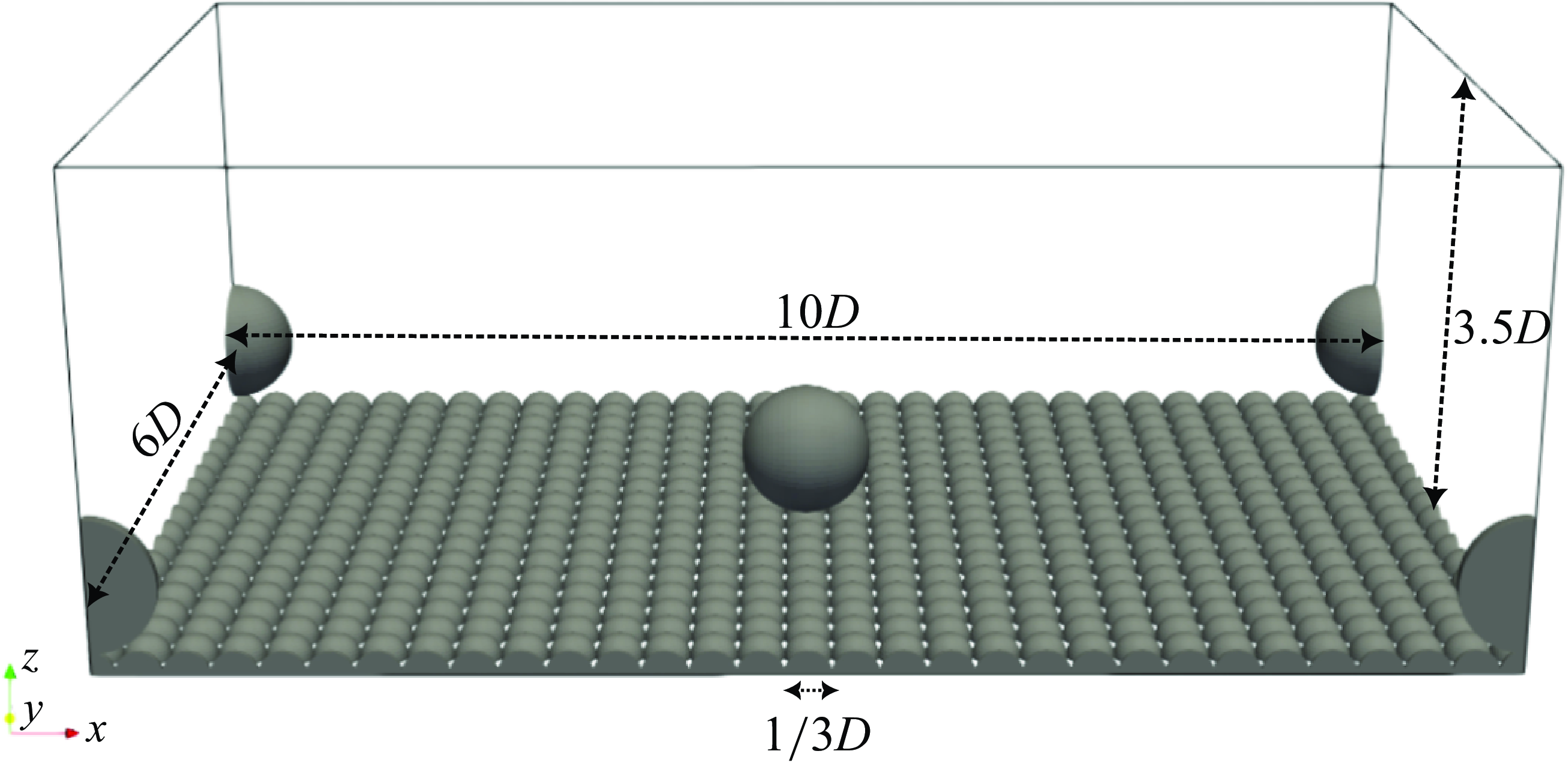
As in the experimental work, the boulders and the rough bed are assumed to be immobile with diameters $D = 5.5$
cm and
$D = 5.5$
cm and $d_{rb} = 1.83$
cm respectively. The relative submergence
$d_{rb} = 1.83$
cm respectively. The relative submergence $RS=h/D = 3.5$
(i.e. ratio between the water depth and the boulders diameter) corresponds to the second regime (i.e. low RS) according to the classification of Nikora et al. (Reference Nikora, Goring, McEwan and Griffiths2001), where the boulders significantly influence the water column without interacting with the free surface. The diagonal boulder spacing
$RS=h/D = 3.5$
(i.e. ratio between the water depth and the boulders diameter) corresponds to the second regime (i.e. low RS) according to the classification of Nikora et al. (Reference Nikora, Goring, McEwan and Griffiths2001), where the boulders significantly influence the water column without interacting with the free surface. The diagonal boulder spacing $\varDelta _d/D$
= 11.67 corresponds to the isolated regime in which the wake of one boulder has a limited influence on the boulder downstream. The Reynolds number
$\varDelta _d/D$
= 11.67 corresponds to the isolated regime in which the wake of one boulder has a limited influence on the boulder downstream. The Reynolds number $Re_h$
= 150 500 and Froude number
$Re_h$
= 150 500 and Froude number $Fr = 0.567$
are maintained the same to replicate the hydrodynamic conditions of the experiment. Both parameters are based on the water depth
$Fr = 0.567$
are maintained the same to replicate the hydrodynamic conditions of the experiment. Both parameters are based on the water depth $h = 0.193$
m defined as the distance from the top of the rough bed hemispheres to the water surface, and the bulk velocity
$h = 0.193$
m defined as the distance from the top of the rough bed hemispheres to the water surface, and the bulk velocity $U_b = 0.78$
m s−1 considered as the cross-sectional mean velocity excluding volumes occupied by the boulders and the rough bed. Since no deformation of the free surface was observed in the experiment, a symmetry boundary condition is employed at the top boundary. Only the rough bed configuration used in this study was changed compared with the experiment by arranging one layer of hemispheres in a cubic pattern, as also performed in the work of Manes et al. (Reference Manes, Pokrajac, McEwan and Nikora2009); Fang et al. (Reference Fang, Han, He and Dey2018) and Bomminayuni & Stoesser (Reference Bomminayuni and Stoesser2011).
$U_b = 0.78$
m s−1 considered as the cross-sectional mean velocity excluding volumes occupied by the boulders and the rough bed. Since no deformation of the free surface was observed in the experiment, a symmetry boundary condition is employed at the top boundary. Only the rough bed configuration used in this study was changed compared with the experiment by arranging one layer of hemispheres in a cubic pattern, as also performed in the work of Manes et al. (Reference Manes, Pokrajac, McEwan and Nikora2009); Fang et al. (Reference Fang, Han, He and Dey2018) and Bomminayuni & Stoesser (Reference Bomminayuni and Stoesser2011).
The laboratory experiment used for comparison was conducted in a flume with a rectangular cross-section and an aspect ratio of $B/h \approx 5$
, where
$B/h \approx 5$
, where $B$
is the channel width. While corner-induced secondary currents may arise under these conditions (Nezu & Nakagawa Reference Nezu and Nakagawa1993), their influence is expected to be limited compared with the spanwise heterogeneity induced by the boulder array. In the simulations, sidewall effects are not considered, and periodic boundary conditions are applied in the spanwise direction to replicate the core region of the experimental set-up. Moreover, the streamwise and spanwise dimensions of the computational domain are consistent with the experimental configuration and are sufficient to resolve large-scale streamwise turbulent structures, as demonstrated by the decay of the velocity autocorrelation functions to zero within less than half the domain length (see Liu et al. (Reference Liu, Stoesser, Fang, Papanicolaou and Tsakiris2017)).
$B$
is the channel width. While corner-induced secondary currents may arise under these conditions (Nezu & Nakagawa Reference Nezu and Nakagawa1993), their influence is expected to be limited compared with the spanwise heterogeneity induced by the boulder array. In the simulations, sidewall effects are not considered, and periodic boundary conditions are applied in the spanwise direction to replicate the core region of the experimental set-up. Moreover, the streamwise and spanwise dimensions of the computational domain are consistent with the experimental configuration and are sufficient to resolve large-scale streamwise turbulent structures, as demonstrated by the decay of the velocity autocorrelation functions to zero within less than half the domain length (see Liu et al. (Reference Liu, Stoesser, Fang, Papanicolaou and Tsakiris2017)).
The governing equations are the three-dimensional, spatially filtered unsteady, incompressible Navier–Stokes equations. They are expressed in the Cartesian coordinates as follows:
 \begin{align}&\qquad\qquad\qquad\qquad \frac {\partial u_i}{\partial x_i} = 0 ,\end{align}
 \begin{align}& \frac {\partial u_i}{\partial t} + u_j \frac {\partial u_i}{\partial x_j} = - \frac {\partial P}{\partial x_i} + \frac {\partial ^2 u_i}{\partial x_j \partial x_j} - \frac {\partial \tau _{ij}}{\partial x_j} + f_{i} ,\end{align}
where $u_i$
are the filtered components of velocity,
$u_i$
are the filtered components of velocity, $P = ({p}/{\rho })-({1}/{3})\delta _{ij}\tau _{kk}$
, with
$P = ({p}/{\rho })-({1}/{3})\delta _{ij}\tau _{kk}$
, with $p$
the filtered pressure,
$p$
the filtered pressure, $\rho$
the fluid density,
$\rho$
the fluid density, $\tau _{ij}$
are the components of the subgrid-scale (SGS) stress tensor and
$\tau _{ij}$
are the components of the subgrid-scale (SGS) stress tensor and $f_i = (f_x,0,0)$
is the driving pressure gradient to maintain a constant discharge when applying periodic boundary conditions. The origin of the coordinate system is placed at the bottom left.
$f_i = (f_x,0,0)$
is the driving pressure gradient to maintain a constant discharge when applying periodic boundary conditions. The origin of the coordinate system is placed at the bottom left.
The SGS tensor is defined as $\tau _{ij} = -2\nu _t S_{ij}$
with
$\tau _{ij} = -2\nu _t S_{ij}$
with $S_{ij} = ({1}/{2}) ( ({\partial u_i}/{\partial x_j}) + ({\partial u_j}/{\partial x_i)})$
the resolved-scale strain-rate tensor. The eddy viscosity is based on the dynamic model with a local average for the constant due to the inhomogeneity of the flow in all directions (Germano et al. Reference Germano, Piomelli, Moin and Cabot1991; Lilly Reference Lilly1992) and is calculated as
$S_{ij} = ({1}/{2}) ( ({\partial u_i}/{\partial x_j}) + ({\partial u_j}/{\partial x_i)})$
the resolved-scale strain-rate tensor. The eddy viscosity is based on the dynamic model with a local average for the constant due to the inhomogeneity of the flow in all directions (Germano et al. Reference Germano, Piomelli, Moin and Cabot1991; Lilly Reference Lilly1992) and is calculated as $\nu _t = C_s \varDelta ^2 |S|$
with
$\nu _t = C_s \varDelta ^2 |S|$
with $|S|=\sqrt {2S_{kl}S_{kl}}$
. This average considers 27 grid points, and the test filter is applied as defined in Germano et al. (Reference Germano, Piomelli, Moin and Cabot1991).
$|S|=\sqrt {2S_{kl}S_{kl}}$
. This average considers 27 grid points, and the test filter is applied as defined in Germano et al. (Reference Germano, Piomelli, Moin and Cabot1991).
The array of boulders and the rough bed are accounted for by the sharp immersed boundary method (IBM) proposed by Gilmanov, Sotiropoulos & Balaras (Reference Gilmanov, Sotiropoulos and Balaras2003) with a discrete forcing, imposing a local direct boundary condition. For high Reynolds numbers, using an IBM implies the challenge of coping with thin boundary layers without the possibility of refining the grid in the wall-normal direction (Verzicco Reference Verzicco2023). This causes the impossibility of resolving the wall and therefore the use of an appropriate wall modelling approach becomes critical for the accuracy of the results. Hence, the wall model proposed in Cabot & Moin (Reference Cabot and Moin2000) and Wang & Moin (Reference Wang and Moin2002) is used for the boulders and the rough bed. This wall model is based on the following boundary-layer equation at the IB nodes (Verzicco Reference Verzicco2023):
 \begin{equation} \frac {1}{\rho } \frac {\partial }{\partial l} \left ( \left ( \mu + \mu _t \right ) \frac {\partial u_s}{\partial l} \right ) = - \frac {1}{\rho } \frac {\partial p}{\partial s} + \frac {\partial u_s}{\partial t} + \frac {\partial u_l u_s}{\partial s}, \end{equation}
where $l$
and
$l$
and $s$
are directions normal and tangential to the wall, respectively, and
$s$
are directions normal and tangential to the wall, respectively, and $\mu _t$
is the turbulent viscosity. Neglecting the right-hand side terms of (2.3), the equilibrium stress balance model is obtained
$\mu _t$
is the turbulent viscosity. Neglecting the right-hand side terms of (2.3), the equilibrium stress balance model is obtained
 \begin{equation} \frac {1}{\rho } \frac {\partial }{\partial l} \left ( \left (\mu + \mu _t\right ) \frac {\partial u_s}{\partial l} \right ) = 0 ,\end{equation}
and the turbulent viscosity is given by the mixing length model with near-wall damping written as
 \begin{equation} \mu _{t} = \mu \kappa l^{+} \left (1 - e^{\frac {-l^{+}}{19}}\right )^{2} ,\end{equation}
where $l^+ = u_* l/\nu$
,
$l^+ = u_* l/\nu$
, $u_*$
is the friction velocity and
$u_*$
is the friction velocity and $\kappa = 0.41$
is the von Kármán constant. Equation (2.4) is solved iteratively for
$\kappa = 0.41$
is the von Kármán constant. Equation (2.4) is solved iteratively for $u_*$
using the Newton–Raphson method (Kang et al. Reference Kang, Lightbody, Hill and Sotiropoulos2011).
$u_*$
using the Newton–Raphson method (Kang et al. Reference Kang, Lightbody, Hill and Sotiropoulos2011).
The Cartesian uniform numerical grid of 33.3 million nodes consists of $501 \times 301 \times 221$
points in the streamwise (
$501 \times 301 \times 221$
points in the streamwise ( $x$
), spanwise (
$x$
), spanwise ( $y$
) and vertical (
$y$
) and vertical ( $z$
) directions, respectively. Using the near-bed effective shear velocity (i.e. subtracting the shear stress borne by roughness elements as pressure and viscous drag) the grid resolution in wall units is
$z$
) directions, respectively. Using the near-bed effective shear velocity (i.e. subtracting the shear stress borne by roughness elements as pressure and viscous drag) the grid resolution in wall units is $\Delta x^+=\Delta y^+=\Delta z^+=45$
. The total friction velocity
$\Delta x^+=\Delta y^+=\Delta z^+=45$
. The total friction velocity $u_*$
= 0.082 m s−1 is a result of the simulation and is computed based on the pressure gradient needed to maintain a constant discharge. The non-dimensional time step is
$u_*$
= 0.082 m s−1 is a result of the simulation and is computed based on the pressure gradient needed to maintain a constant discharge. The non-dimensional time step is $\Delta t = 0.01$
(0.0007 s) based on the bulk velocity and the boulder diameter.
$\Delta t = 0.01$
(0.0007 s) based on the bulk velocity and the boulder diameter.
The filtered Navier–Stokes equations are solved using a dual time-stepping artificial compressibility scheme, employing a second-order accurate finite-volume method on a non-staggered computational grid. The discrete equations are advanced in time by the pressure-based implicit preconditioner of Sotiropoulos & Constantinescu (Reference Sotiropoulos and Constantinescu1997), enhanced with local time stepping. Applications and performance of this model have been tested and discussed in detail in a series of previous papers, in which the accuracy of the methods has been demonstrated by comparisons with detailed available experimental data (see Paik, Escauriaza & Sotiropoulos Reference Paik, Escauriaza and Sotiropoulos2007; Escauriaza & Sotiropoulos Reference Escauriaza and Sotiropoulos2011a ,Reference Escauriaza and Sotiropoulos b ; Gajardo, Escauriaza & Ingram Reference Gajardo, Escauriaza and Ingram2019; Gotelli et al. Reference Gotelli, Musa, Guala and Escauriaza2019; Sandoval et al. Reference Sandoval, Mignot, Mao, Pastén, Bolster and Escauriaza2019; Barros & Escauriaza Reference Barros and Escauriaza2024 for details).
3. Time-averaged and instantaneous flow field
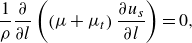
A brief description of the time-averaged and instantaneous flow obtained by LES, comparing the results with the experiments of Papanicolaou et al. (Reference Papanicolaou, Kramer, Tsakiris, Stoesser, Bomminayuni and Chen2012) is presented in this section.
3.1. Comparison with experimental data
Mean velocity and root mean square of the streamwise velocity fluctuations obtained from the LES are compared with the experimental data of Papanicolaou et al. (Reference Papanicolaou, Kramer, Tsakiris, Stoesser, Bomminayuni and Chen2012) and the simulation results of Liu et al. (Reference Liu, Stoesser, Fang, Papanicolaou and Tsakiris2017) in figure 2.
Comparison between our (black continuous line), the experimental data of Papanicolaou et al. (Reference Papanicolaou, Kramer, Tsakiris, Stoesser, Bomminayuni and Chen2012) (red circles) and the LES of Liu et al. (Reference Liu, Stoesser, Fang, Papanicolaou and Tsakiris2017) (black dashed line). Top - non-dimensional mean velocity. Bottom - non-dimensional root mean square of the streamwise velocity fluctuations. The data correspond to different locations along the centreline of the computational domain.
The results show that LES reproduces the mean velocity profiles within the array of boulders and particularly the wake and the average velocity gradients. A near wake is clearly observed downstream of the first boulder with a peak of $\sqrt {\overline {u^{\prime}u^{\prime}}}$
at roughly the boulder height. Further downstream, the flow recovers and slowly tends towards a rough bed boundary-layer profile before reaching the next boulder. The model is able to correctly predict the deficit in the velocity profiles occurring in the wake of the boulders, as well as the increase in the root mean square of the streamwise velocity fluctuation around the boulders crest. This is an indicator of the quality of the IBM method implemented here. The friction velocity obtained here (
$\sqrt {\overline {u^{\prime}u^{\prime}}}$
at roughly the boulder height. Further downstream, the flow recovers and slowly tends towards a rough bed boundary-layer profile before reaching the next boulder. The model is able to correctly predict the deficit in the velocity profiles occurring in the wake of the boulders, as well as the increase in the root mean square of the streamwise velocity fluctuation around the boulders crest. This is an indicator of the quality of the IBM method implemented here. The friction velocity obtained here ( $u_*$
= 0.082 m s−1) is in very good agreement with the averaged values reported in the experiments of Papanicolaou et al. (Reference Papanicolaou, Kramer, Tsakiris, Stoesser, Bomminayuni and Chen2012) (
$u_*$
= 0.082 m s−1) is in very good agreement with the averaged values reported in the experiments of Papanicolaou et al. (Reference Papanicolaou, Kramer, Tsakiris, Stoesser, Bomminayuni and Chen2012) ( $u_*$
= 0.075 m s−1) and the simulation of Liu et al. (Reference Liu, Stoesser, Fang, Papanicolaou and Tsakiris2017) (
$u_*$
= 0.075 m s−1) and the simulation of Liu et al. (Reference Liu, Stoesser, Fang, Papanicolaou and Tsakiris2017) ( $u_*$
= 0.079 m s−1), with only minor differences likely due to variations in the rough bed configuration.
$u_*$
= 0.079 m s−1), with only minor differences likely due to variations in the rough bed configuration.
3.2. Mean flow and second-order statistics
Figure 3 presents the time-averaged velocity magnitude and streamlines in some horizontal and vertical planes as well as some cross-sections. The four horizontal planes correspond to elevations at one, two and three quarters of the height of the boulder (figure 3
b–d) and slightly above the rough bed (figure 3
a). The two vertical planes are located at the middle of the central boulder (figure 3
e) and with a centre slightly shifted in the transverse direction (figure 3
f). Finally, the three cross-sections are located upstream, at the centre and downstream the central boulder respectively (figure 3
g–i). The streamlines show similar patterns of the flow past spheres on a smooth bed and a rough bed with different packing, where separation occurs upstream at mid-boulder elevation (Papanicolaou et al. Reference Papanicolaou, Kramer, Tsakiris, Stoesser, Bomminayuni and Chen2012; Liu et al. Reference Liu, Stoesser, Fang, Papanicolaou and Tsakiris2017). The flow accelerates above and around the spheres producing a low-velocity region downstream. In the present work the rough bed significantly influences the wake of the boulders where a loss of coherence is observed compared with a smooth bed (Hajimirzaie et al. Reference Hajimirzaie, Tsakiris, Buchholz and Papanicolaou2014) since a low-velocity zone with no vertical recirculation is generated downstream of the boulders, as shown in figure 3(e). This occurs because the flow accelerates around the boulders producing a vertically oriented flow in the wake. Therefore, even when a recirculating region is observed in the wake of the boulders in the horizontal planes (figure 3
a–d), it is influenced by the vertical flow coming from the sides of the boulders (figure 3
e). The rough bed also deviates the streamlines compared with the mid-boulder elevation, between the small hemispheres, which is observed in the horizontal plane slightly above the rough bed $(z-r_{rb})/D = 0.06$
(figure 3
a). The extension of the mean low-velocity region located downstream the boulders agrees with the results reported by Liu et al. (Reference Liu, Stoesser, Fang, Papanicolaou and Tsakiris2017) and it is about two boulder diameters.
$(z-r_{rb})/D = 0.06$
(figure 3
a). The extension of the mean low-velocity region located downstream the boulders agrees with the results reported by Liu et al. (Reference Liu, Stoesser, Fang, Papanicolaou and Tsakiris2017) and it is about two boulder diameters.
Streamlines and non-dimensional time-averaged velocity magnitude at four horizontal, two vertical and three cross-sectional planes. The horizontal planes correspond to $(z-r_{rb})/D = 0.06$
(a),
$(z-r_{rb})/D = 0.06$
(a), $0.25$
(b),
$0.25$
(b), $0.5$
(c) and
$0.5$
(c) and $0.75$
(d). The vertical planes include
$0.75$
(d). The vertical planes include $y/D=3$
(e) and
$y/D=3$
(e) and $3.18$
(f). The cross-sectional planes are located at
$3.18$
(f). The cross-sectional planes are located at $x/D=2$
(g),
$x/D=2$
(g), $5$
(h) and
$5$
(h) and $7$
(f). The velocity magnitude is computed considering only the components within the planes.
$7$
(f). The velocity magnitude is computed considering only the components within the planes.
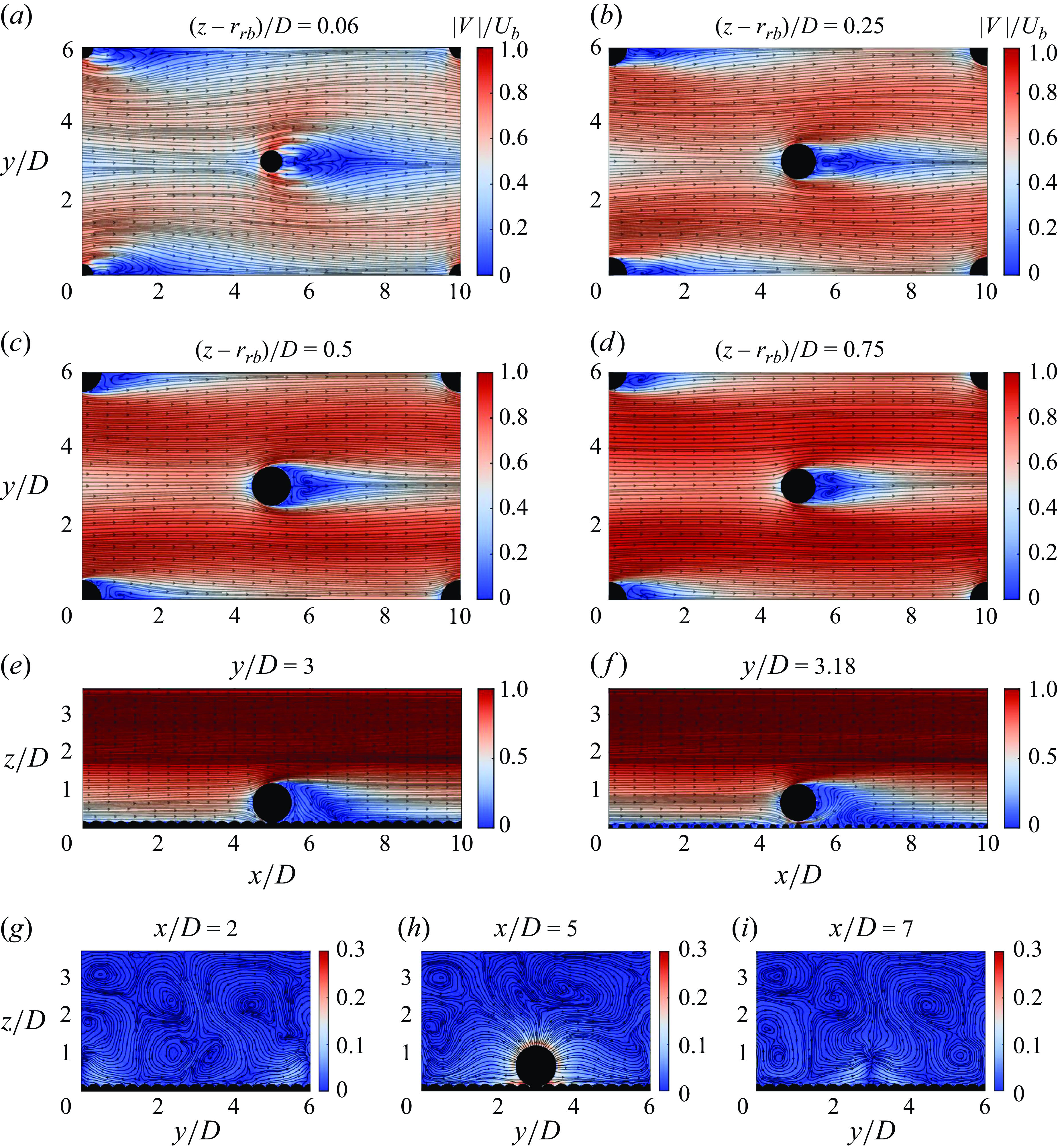
The cross-sections of figures 3(g)–3(i) show secondary flow induced by the boulders. In addition, the longitudinal-averaged mean flow in the cross-section is also given in figure 4. Secondary currents of Prandtl second type emerging from the boulders heterogeneity in the transverse direction are observed (Nikora & Roy Reference Nikora and Roy2012; Anderson et al. Reference Anderson, Barros, Christensen and Awasthi2015). Counter-rotating cells with upward flow at the boulder location and downward flow between the boulders in the transverse direction are depicted in figure 4. The size of secondary current (SC) cells is larger than the boulder diameter and scales with the transverse spacing between boulders as has been observed in previous studies (Zampiron, Cameron & Nikora Reference Zampiron, Cameron and Nikora2020).
Cross-section distribution of mean streamwise velocity $\overline {u}/U_b$
with (
$\overline {u}/U_b$
with ( $\overline {v}/U_b$
,
$\overline {v}/U_b$
, $\overline {w}/U_b$
) vectors. To show the overall presence of secondary currents, all velocities are averaged in the longitudinal direction. The scale of the arrow is indicated in the figure.
$\overline {w}/U_b$
) vectors. To show the overall presence of secondary currents, all velocities are averaged in the longitudinal direction. The scale of the arrow is indicated in the figure.
The primary component of non-dimensional shear stress $-\overline {u^{\prime}w^{\prime}}$
and the TKE are shown in figure 5. The vertical plane at the middle of the central boulder is depicted where clear maxima of
$-\overline {u^{\prime}w^{\prime}}$
and the TKE are shown in figure 5. The vertical plane at the middle of the central boulder is depicted where clear maxima of $-\overline {u^{\prime}w^{\prime}}$
and TKE can be observed at the top of the boulders, and a local peak just above the rough bed can also be identified. The two horizontal planes show the two vertical locations indicated by the dashed lines in figure 5. The horizontal plane located at the boulders crest illustrates the high TKE magnitude together with high shear stress downstream the boulders top, which has been widely observed in previous studies (Hajimirzaie et al. Reference Hajimirzaie, Tsakiris, Buchholz and Papanicolaou2014; Liu et al. Reference Liu, Stoesser, Fang, Papanicolaou and Tsakiris2017). Maximum values found at the boulders crest result from the shear layer produced above the spheres, separating the high-velocity flow above the boulders and the low velocity in the downstream wake. The observed TKE maximum mainly results from high streamwise velocity fluctuations. Conversely, in the region between the rough bed and the top of the boulders, beneath the shear layer and within the wake, low values of TKE and
$-\overline {u^{\prime}w^{\prime}}$
and TKE can be observed at the top of the boulders, and a local peak just above the rough bed can also be identified. The two horizontal planes show the two vertical locations indicated by the dashed lines in figure 5. The horizontal plane located at the boulders crest illustrates the high TKE magnitude together with high shear stress downstream the boulders top, which has been widely observed in previous studies (Hajimirzaie et al. Reference Hajimirzaie, Tsakiris, Buchholz and Papanicolaou2014; Liu et al. Reference Liu, Stoesser, Fang, Papanicolaou and Tsakiris2017). Maximum values found at the boulders crest result from the shear layer produced above the spheres, separating the high-velocity flow above the boulders and the low velocity in the downstream wake. The observed TKE maximum mainly results from high streamwise velocity fluctuations. Conversely, in the region between the rough bed and the top of the boulders, beneath the shear layer and within the wake, low values of TKE and $-\overline {u^{\prime}w^{\prime}}$
exist. Slightly above the rough bed and between the boulders, spanning from at least
$-\overline {u^{\prime}w^{\prime}}$
exist. Slightly above the rough bed and between the boulders, spanning from at least $3.5\lt y/D\lt 5.5$
or
$3.5\lt y/D\lt 5.5$
or $0.5\lt y/D\lt 2.5$
in the transverse direction, where the streamwise velocity is high, TKE is high as well as
$0.5\lt y/D\lt 2.5$
in the transverse direction, where the streamwise velocity is high, TKE is high as well as $-\overline {u^{\prime}w^{\prime}}$
. These conditions might have direct implications for bedload transport and for the hydrodynamic stresses acting on particles at the bed. We anticipate that sediments could deposit in low streamwise velocity and
$-\overline {u^{\prime}w^{\prime}}$
. These conditions might have direct implications for bedload transport and for the hydrodynamic stresses acting on particles at the bed. We anticipate that sediments could deposit in low streamwise velocity and $-\overline {u^{\prime}w^{\prime}}$
regions of the wake and be transported in high streamwise velocity and
$-\overline {u^{\prime}w^{\prime}}$
regions of the wake and be transported in high streamwise velocity and $-\overline {u^{\prime}w^{\prime}}$
regions between the boulders in the transverse direction. Recently, Liu et al. (Reference Liu, Tang, Huang, Stoesser and Fang2024) found similar values of low and high
$-\overline {u^{\prime}w^{\prime}}$
regions between the boulders in the transverse direction. Recently, Liu et al. (Reference Liu, Tang, Huang, Stoesser and Fang2024) found similar values of low and high $-\overline {u^{\prime}w^{\prime}}$
and TKE downstream and between the boulders, respectively, for low and intermediate Froude numbers and a much lower relative submergence
$-\overline {u^{\prime}w^{\prime}}$
and TKE downstream and between the boulders, respectively, for low and intermediate Froude numbers and a much lower relative submergence $h/D=0.8$
, indicating that these patterns persist even when the boulders emerge from the water and the free-surface effect is limited. Local peaks of TKE are also observed in the horizontal plane just above the rough bed, indicating a local increase of the turbulence at the top of the hemispheres as previously observed by Fang et al. (Reference Fang, Han, He and Dey2018).
$h/D=0.8$
, indicating that these patterns persist even when the boulders emerge from the water and the free-surface effect is limited. Local peaks of TKE are also observed in the horizontal plane just above the rough bed, indicating a local increase of the turbulence at the top of the hemispheres as previously observed by Fang et al. (Reference Fang, Han, He and Dey2018).
(a) Primary component of non-dimensional shear stress and (b) non-dimensional TKE. The vertical plane is located at the middle of the central boulder $y/D=3$
whereas the two horizontal planes correspond to the top of the boulders
$y/D=3$
whereas the two horizontal planes correspond to the top of the boulders $(z-r_{rb})/D = 1$
and just above the rough bed
$(z-r_{rb})/D = 1$
and just above the rough bed $(z-r_{rb})/D \approx 0$
where shear stress and TKE reach their local and global peaks (see dashed lines at the top).
$(z-r_{rb})/D \approx 0$
where shear stress and TKE reach their local and global peaks (see dashed lines at the top).
To assess the scale of spatial variations of the time-averaged streamwise velocity, turbulent stresses and TKE along the streamwise and spanwise directions just above the rough bed are shown in figure 6 along with the standard deviation. Two characteristic length scales are clearly visible in both directions, a larger one induced by the boulders and a smaller produced by the rough bed. Since the flow accelerates in the vicinity of the boulders, there is a peak of transverse-averaged streamwise velocity at the boulder locations denoted with a letter B in figure 6(a). Conversely, at the same location a minimum of $-\overline {u^{\prime}w^{\prime}}$
and TKE are observed as these quantities decrease (see figures 3 and 5). All longitudinal-averaged quantities reach a minimum at the boulders (figure 6
b), resulting from the low velocities and Reynolds stresses in the wake. Maximum values of longitudinal-averaged velocity, TKE and shear stress are observed in the high-velocity region between the boulders in the transverse direction (figure 6
b). Since bedload transport occurs mostly in the streamwise direction, it may be inferred that the streamwise-averaged Reynolds shear-stress profile depicted in figure 6(b) would contribute to erosion between the boulders, where high values of turbulent shear stresses exist, and deposition in the wake where low values are observed. This is consistent with sediment deposition patches observed within the same array of boulders by Papanicolaou et al. (Reference Papanicolaou, Tsakiris, Wyssmann and Kramer2018).
$-\overline {u^{\prime}w^{\prime}}$
and TKE are observed as these quantities decrease (see figures 3 and 5). All longitudinal-averaged quantities reach a minimum at the boulders (figure 6
b), resulting from the low velocities and Reynolds stresses in the wake. Maximum values of longitudinal-averaged velocity, TKE and shear stress are observed in the high-velocity region between the boulders in the transverse direction (figure 6
b). Since bedload transport occurs mostly in the streamwise direction, it may be inferred that the streamwise-averaged Reynolds shear-stress profile depicted in figure 6(b) would contribute to erosion between the boulders, where high values of turbulent shear stresses exist, and deposition in the wake where low values are observed. This is consistent with sediment deposition patches observed within the same array of boulders by Papanicolaou et al. (Reference Papanicolaou, Tsakiris, Wyssmann and Kramer2018).
Longitudinal and transverse profiles of near-bed time-averaged streamwise velocity, Reynolds shear stress and TKE. (a) Quantities averaged over transverse lines and (b) over longitudinal lines. The black curve shows the average while the grey area is delimited by the average $\pm$
the standard deviation. The dashed grey lines depict the position of the crest of the hemispheres of the rough bed.
$\pm$
the standard deviation. The dashed grey lines depict the position of the crest of the hemispheres of the rough bed.
3.3. Instantaneous flow: vorticity and isosurfaces of Q
To show the complex 3-D instantaneous flow around the boulders and the rough bed, in figure 7 we show a snapshot of non-dimensional spanwise and vertical vorticity and magnitude (including all three components). The vertical plane is located at the middle of the central boulder, while the two horizontal planes correspond to the mid-boulder elevation and just above the rough bed. The instantaneous vorticity patterns observed in the wake of the boulders in figure 7 are in good agreement with the observations of Papanicolaou et al. (Reference Papanicolaou, Kramer, Tsakiris, Stoesser, Bomminayuni and Chen2012) and Zhao et al. (Reference Zhao, Liu, Li, Wei, Luo and Fan2016), and the vortices induced by the rough bed also agree with the findings of Fang et al. (Reference Fang, Han, He and Dey2018) and Bomminayuni & Stoesser (Reference Bomminayuni and Stoesser2011). The spanwise vorticity and magnitude show the shear layer that separates the high- and low-velocity regions around the boulders, and the strong vorticity produced in the wake of the central boulder. The horizontal planes allow the comparison between two different elevations that correspond to the centre of the boulders and slightly above the rough bed where competing processes control the instantaneous flow dynamics. Namely, at the mid-boulder elevation, the vorticity patterns are mainly a result from the boulders wake. Close to the rough bed, local peaks of positive and negative vertical vorticity are observed at each side of the top of the hemispheres together with peaks of vorticity magnitude slightly above their crests. A decrease of vorticity is also observed in the wake of the boulders close to the rough bed. Figure 7 also illustrates the ability of LES to reproduce the complex turbulent dynamics induced by the array of boulders and the interactions with the rough bed.
Non-dimensional instantaneous resolved flow field: (a) vorticity normal to the plane and (b) vorticity magnitude. The vertical plane (top) is located at the middle of the central boulder $y/D=3$
whereas the two horizontal planes (centre and bottom) correspond to the mid-boulder elevation
$y/D=3$
whereas the two horizontal planes (centre and bottom) correspond to the mid-boulder elevation $(z-r_{rb})/D = 0.5$
(centre) and just above the rough bed
$(z-r_{rb})/D = 0.5$
(centre) and just above the rough bed $(z-r_{rb})/D \approx 0$
(bottom).
$(z-r_{rb})/D \approx 0$
(bottom).
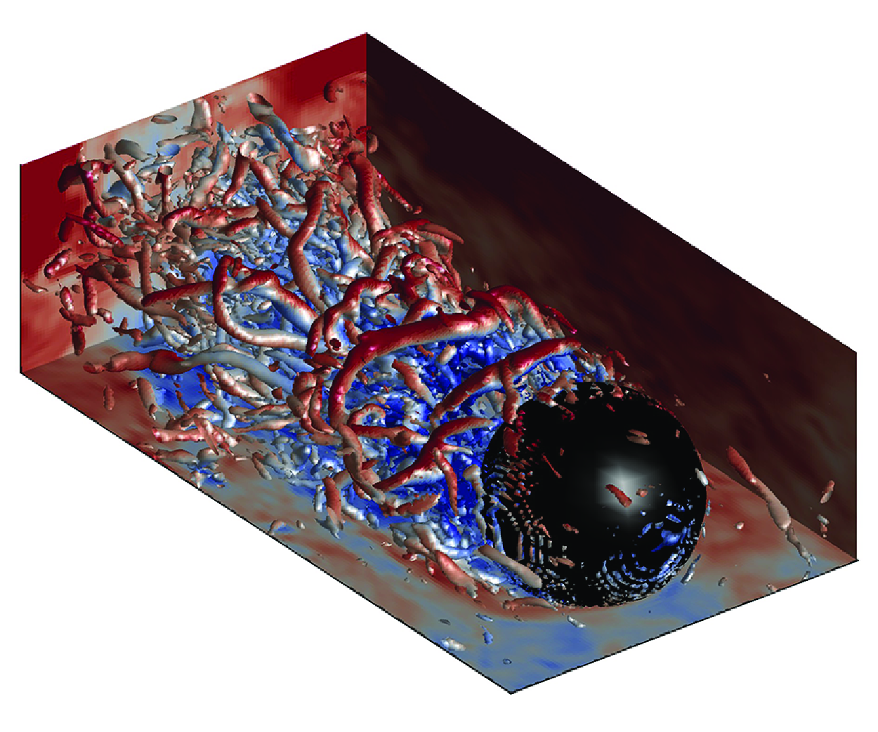
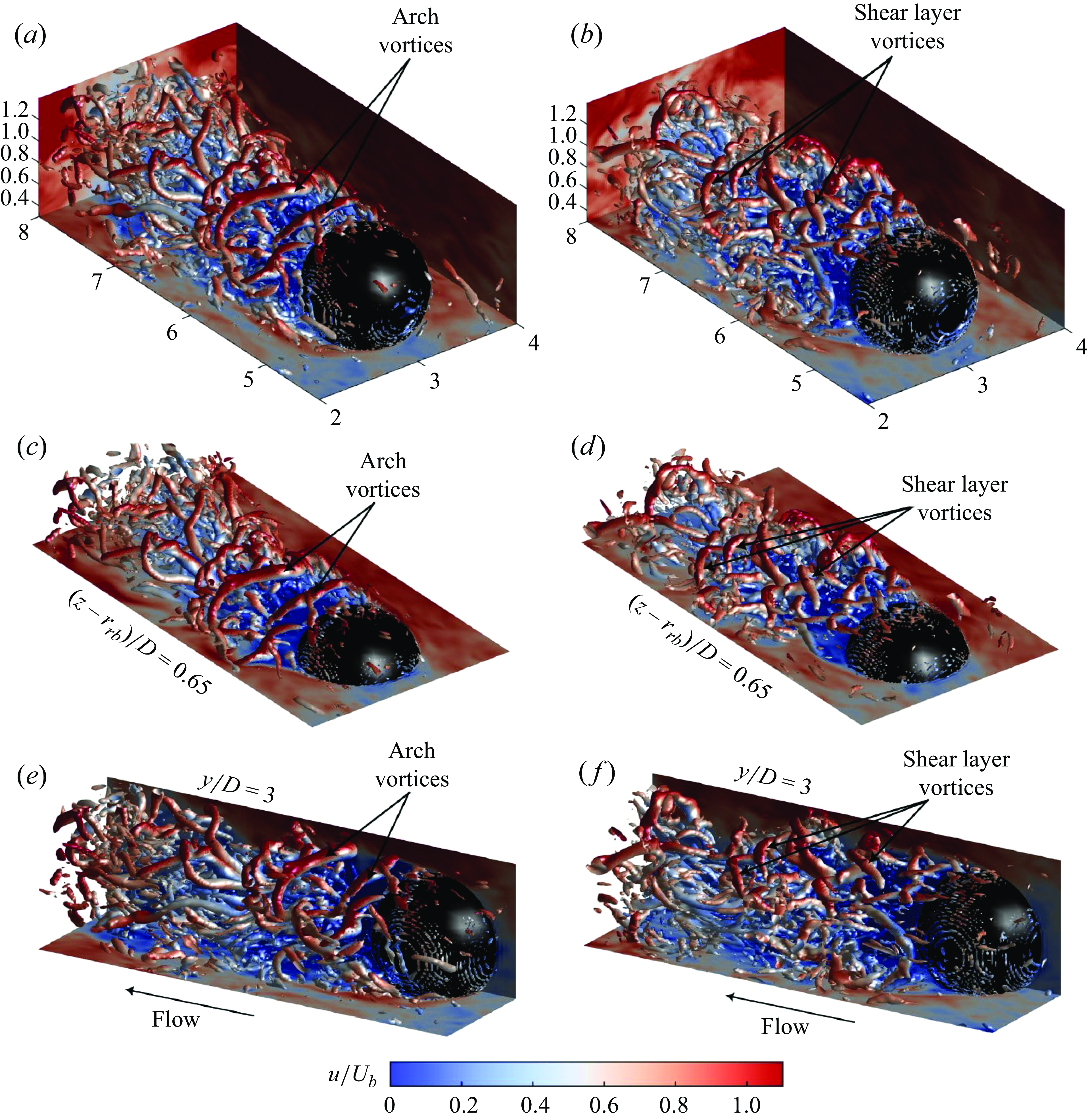
The Q-criterion is used to detect coherent structures and visualise the 3-D instantaneous structure of the wake, identifying regions where the local rotation rate is larger than the strain rate, given by the second invariant of the velocity gradient tensor $Q=({1}/{2})(\varOmega _{ij} \varOmega _{ij} - S_{ij}S_{ij})\gt 0$
. Figure 8 shows isosurfaces of non-dimensional
$Q=({1}/{2})(\varOmega _{ij} \varOmega _{ij} - S_{ij}S_{ij})\gt 0$
. Figure 8 shows isosurfaces of non-dimensional $Q = 15$
downstream the central boulder, coloured by the non-dimensional streamwise velocity. Quantities are normalised using the bulk velocity and the boulder diameter. Two snapshots separated by one non-dimensional time (i.e.
$Q = 15$
downstream the central boulder, coloured by the non-dimensional streamwise velocity. Quantities are normalised using the bulk velocity and the boulder diameter. Two snapshots separated by one non-dimensional time (i.e. $h/U_b$
) are shown in figure 8 where (a), (c) and (e) correspond to the first instant and b,d and f to the second. Figures 8(a), 8(b) show almost the entire wake from slightly above the rough bed (
$h/U_b$
) are shown in figure 8 where (a), (c) and (e) correspond to the first instant and b,d and f to the second. Figures 8(a), 8(b) show almost the entire wake from slightly above the rough bed ( $(z-r_{rb})/D=0.13$
), whereas figures 8(c), 8(d) only show the top region closer to the shear layer (cut by a horizontal plane at
$(z-r_{rb})/D=0.13$
), whereas figures 8(c), 8(d) only show the top region closer to the shear layer (cut by a horizontal plane at $(z-r_{rb})/D=0.65$
) and figures 8(e), 8(f) show the middle of the wake, cut by a vertical plane at
$(z-r_{rb})/D=0.65$
) and figures 8(e), 8(f) show the middle of the wake, cut by a vertical plane at $y/D=3$
. The slices of streamwise velocity allow a clear visualisation of the wake and the vortices that emerge from the shear layer. Arch vortices are identified in the proximity of the boulder as proposed by Hajimirzaie et al. (Reference Hajimirzaie, Tsakiris, Buchholz and Papanicolaou2014). These structures are primarily vertically oriented and travel downstream before being fragmented, only surviving approximately two diameters downstream. Shear layer vortices of horseshoe shape are also observed as indicated in figure 8, with their heads oriented downstream and at a higher elevation and therefore moving faster than their legs. These vortices have been widely observed in previous studies in the wake of spheres and wall-mounted hemispheres (Liu et al. Reference Liu, Stoesser, Fang, Papanicolaou and Tsakiris2017; Kamble & Girimaji Reference Kamble and Girimaji2020; Li et al. Reference Li, Qiu, Shao, Liu, Fu, Tao and Liu2022). These structures emerge from the shear layer and therefore exist far from the bed in a zone of high streamwise velocity, TKE and Reynolds shear stresses contributing to the production of TKE
$y/D=3$
. The slices of streamwise velocity allow a clear visualisation of the wake and the vortices that emerge from the shear layer. Arch vortices are identified in the proximity of the boulder as proposed by Hajimirzaie et al. (Reference Hajimirzaie, Tsakiris, Buchholz and Papanicolaou2014). These structures are primarily vertically oriented and travel downstream before being fragmented, only surviving approximately two diameters downstream. Shear layer vortices of horseshoe shape are also observed as indicated in figure 8, with their heads oriented downstream and at a higher elevation and therefore moving faster than their legs. These vortices have been widely observed in previous studies in the wake of spheres and wall-mounted hemispheres (Liu et al. Reference Liu, Stoesser, Fang, Papanicolaou and Tsakiris2017; Kamble & Girimaji Reference Kamble and Girimaji2020; Li et al. Reference Li, Qiu, Shao, Liu, Fu, Tao and Liu2022). These structures emerge from the shear layer and therefore exist far from the bed in a zone of high streamwise velocity, TKE and Reynolds shear stresses contributing to the production of TKE $-\overline {u^{\prime}w^{\prime}} ({\partial \overline {u}}/{\partial z})$
. Consequently, they may also play an important role in suspended transport of sediments and nutrients. The figures and animations reveal a rich dynamics, in which shear layer vortices are advected downstream while deformed by high shear, and sometimes breaking into longitudinal structures, which are elongated and advected further downstream.
$-\overline {u^{\prime}w^{\prime}} ({\partial \overline {u}}/{\partial z})$
. Consequently, they may also play an important role in suspended transport of sediments and nutrients. The figures and animations reveal a rich dynamics, in which shear layer vortices are advected downstream while deformed by high shear, and sometimes breaking into longitudinal structures, which are elongated and advected further downstream.
Sequence of non-dimensional Q isosurfaces ( $Q = 15$
) show the 3-D instantaneous structure of the wake of the central boulder. The images are coloured by the dimensionless streamwise velocity. The figures at the left and the right are separated by one non-dimensional time (
$Q = 15$
) show the 3-D instantaneous structure of the wake of the central boulder. The images are coloured by the dimensionless streamwise velocity. The figures at the left and the right are separated by one non-dimensional time ( $h/U_b$
). Panels (a) and (b) show the wake slightly above the rough bed
$h/U_b$
). Panels (a) and (b) show the wake slightly above the rough bed $(z-r_{rb})/D=0.13$
; (c) and (d) are sliced through a horizontal plane at
$(z-r_{rb})/D=0.13$
; (c) and (d) are sliced through a horizontal plane at $(z-r_{rb})/D=0.65$
and (e) and (f) by a vertical plane at
$(z-r_{rb})/D=0.65$
and (e) and (f) by a vertical plane at $y/D=3$
. The locations of prominent arch and shear layer vortices are indicated by arrows.
$y/D=3$
. The locations of prominent arch and shear layer vortices are indicated by arrows.
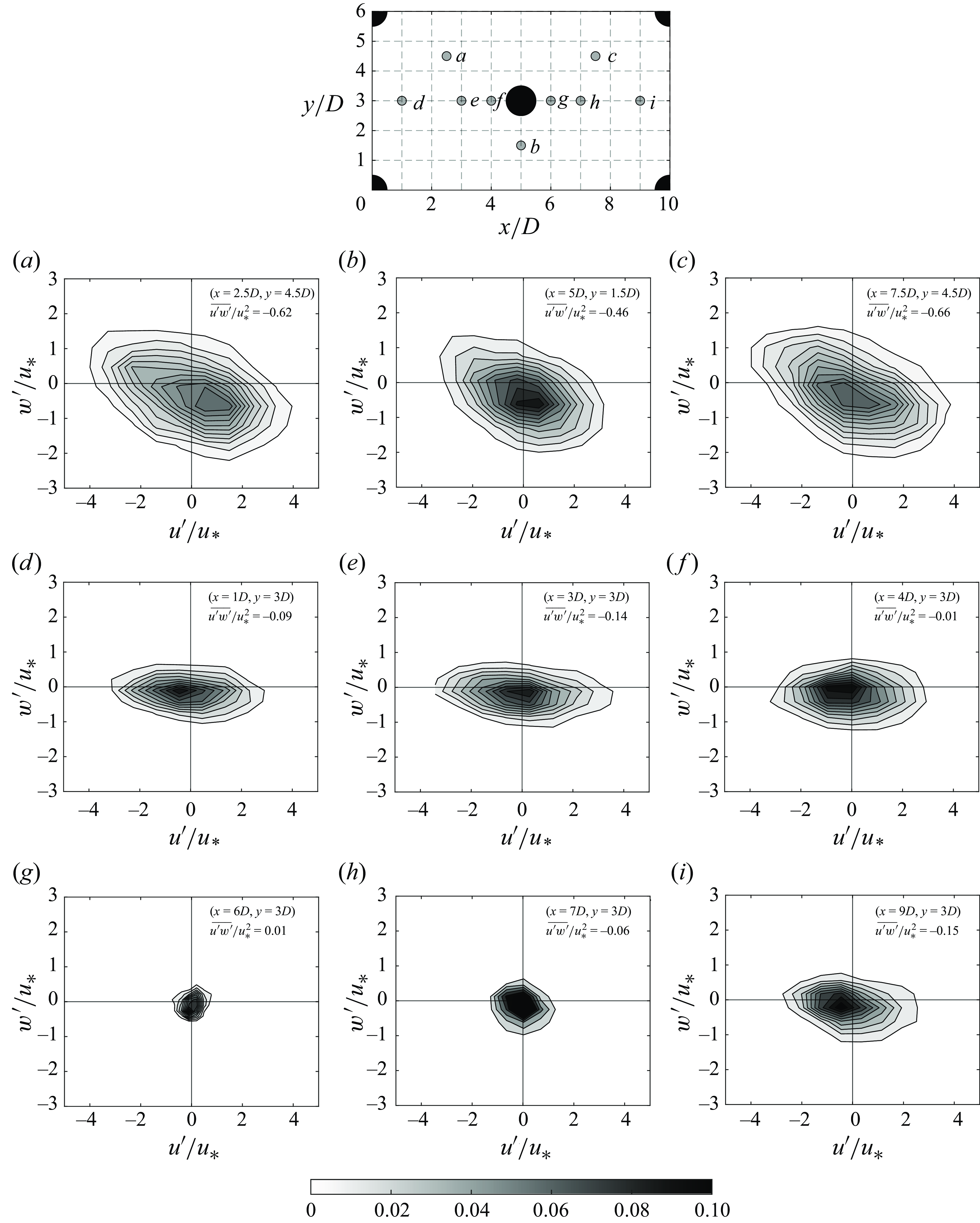
3.4. Quadrant analysis of near-bed Reynolds shear stress
From the simulations we can also analyse the distribution of near-bed turbulent events through the joint frequency distribution of $u^{\prime}$
and
$u^{\prime}$
and $w^{\prime}$
, as shown in figure 9 at different locations around the central boulder. According to the sign of the streamwise and vertical velocity fluctuations at a given point, the joint frequency of
$w^{\prime}$
, as shown in figure 9 at different locations around the central boulder. According to the sign of the streamwise and vertical velocity fluctuations at a given point, the joint frequency of $u^{\prime}$
and
$u^{\prime}$
and $w^{\prime}$
is sorted in four different quadrants representing outward interactions (Q1,
$w^{\prime}$
is sorted in four different quadrants representing outward interactions (Q1, $u^{\prime} \gt 0$
and
$u^{\prime} \gt 0$
and $w^{\prime} \gt 0$
), ejections (Q2,
$w^{\prime} \gt 0$
), ejections (Q2, $u^{\prime} \lt 0$
and
$u^{\prime} \lt 0$
and $w^{\prime}\gt 0$
), inward interactions (Q3,
$w^{\prime}\gt 0$
), inward interactions (Q3, $u^{\prime} \lt 0$
and
$u^{\prime} \lt 0$
and $w^{\prime} \lt 0$
) and sweeps (Q4,
$w^{\prime} \lt 0$
) and sweeps (Q4, $u^{\prime} \gt 0$
and
$u^{\prime} \gt 0$
and $w^{\prime} \lt 0$
) (Wallace Reference Wallace2016). The joint distributions depicted in figure 9(a,b,c) show elliptically shaped contours with negative slope resulting from the strong negative correlation of
$w^{\prime} \lt 0$
) (Wallace Reference Wallace2016). The joint distributions depicted in figure 9(a,b,c) show elliptically shaped contours with negative slope resulting from the strong negative correlation of $u^{\prime}$
and
$u^{\prime}$
and $w^{\prime}$
in the high-velocity region between the boulders as is typically found in the near-bed region in open-channel flows, where sweeps (Q4) and ejections (Q2) are the dominant contributions to turbulent stresses rather than outward (Q1) and inward (Q3) interactions. Points located upstream (second row, figure 9
d,e,f) and downstream (third row, figure 9
g,h,i) of the boulders, on the other hand, still present a rather elliptical shape with a horizontal slope. This zero axis symmetry implies a very small and close to zero average value of
$w^{\prime}$
in the high-velocity region between the boulders as is typically found in the near-bed region in open-channel flows, where sweeps (Q4) and ejections (Q2) are the dominant contributions to turbulent stresses rather than outward (Q1) and inward (Q3) interactions. Points located upstream (second row, figure 9
d,e,f) and downstream (third row, figure 9
g,h,i) of the boulders, on the other hand, still present a rather elliptical shape with a horizontal slope. This zero axis symmetry implies a very small and close to zero average value of $u^{\prime}w^{\prime}$
compared with the intensity of the observed turbulent fluctuations. This is especially true for points located upstream the boulders (figure 9
d,e,f) since velocity fluctuations are still large there but turbulent stresses are small as positive and negative values of
$u^{\prime}w^{\prime}$
compared with the intensity of the observed turbulent fluctuations. This is especially true for points located upstream the boulders (figure 9
d,e,f) since velocity fluctuations are still large there but turbulent stresses are small as positive and negative values of $u^{\prime}w^{\prime}$
are equally represented. At those locations not only sweeps and ejections become important but also outward and inward interactions as previously observed by Fang et al. (Reference Fang, Liu and Stoesser2017). The important conclusion here is that local turbulent stresses are a good representation of instantaneous events in locally uniform flows due to the strong negative correlation between
$u^{\prime}w^{\prime}$
are equally represented. At those locations not only sweeps and ejections become important but also outward and inward interactions as previously observed by Fang et al. (Reference Fang, Liu and Stoesser2017). The important conclusion here is that local turbulent stresses are a good representation of instantaneous events in locally uniform flows due to the strong negative correlation between $u^{\prime}$
and
$u^{\prime}$
and $w^{\prime}$
(as here within the transverse region between the boulders). However, this statement fails for regions upstream and downstream the boulders where the correlation is low and hence the mean value (i.e. turbulent stresses) no longer correctly represents the instantaneous turbulent events. This was first observed by Nelson et al. (Reference Nelson, Shreve, McLean and Drake1995), who measured near-bed velocities and bedload transport at different distances downstream a backward facing step. They found that sweeps and outward interactions became predominant and contributed more significantly to bedload fluxes, differing from a well-developed boundary layer. A decrease of the correlation between
$w^{\prime}$
(as here within the transverse region between the boulders). However, this statement fails for regions upstream and downstream the boulders where the correlation is low and hence the mean value (i.e. turbulent stresses) no longer correctly represents the instantaneous turbulent events. This was first observed by Nelson et al. (Reference Nelson, Shreve, McLean and Drake1995), who measured near-bed velocities and bedload transport at different distances downstream a backward facing step. They found that sweeps and outward interactions became predominant and contributed more significantly to bedload fluxes, differing from a well-developed boundary layer. A decrease of the correlation between $u^{\prime}$
and
$u^{\prime}$
and $w^{\prime}$
characterised by the existence of a horizontal rather than a large negative slope as the typical behaviour in wall turbulence was also observed by Guan, Agarwal & Chiew (Reference Guan, Agarwal and Chiew2018) in the low-velocity region inside a vertical cavity. This has important consequences since bedload fluxes may be poorly correlated to near-bed shear stress in non-uniform flows (Yager et al. Reference Yager, Venditti, Smith and Schmeeckle2018).
$w^{\prime}$
characterised by the existence of a horizontal rather than a large negative slope as the typical behaviour in wall turbulence was also observed by Guan, Agarwal & Chiew (Reference Guan, Agarwal and Chiew2018) in the low-velocity region inside a vertical cavity. This has important consequences since bedload fluxes may be poorly correlated to near-bed shear stress in non-uniform flows (Yager et al. Reference Yager, Venditti, Smith and Schmeeckle2018).
Joint frequency distributions of near-bed $u^\prime$
and
$u^\prime$
and $w^\prime$
at different locations. The locations in the horizontal plane are depicted in the schematic figure at the top. The position and the value of the turbulent stress at each point is shown inside the panels. First row corresponds to points located between the boulders (high-velocity region), and second and third rows to points located upstream and downstream the central boulder, respectively.
$w^\prime$
at different locations. The locations in the horizontal plane are depicted in the schematic figure at the top. The position and the value of the turbulent stress at each point is shown inside the panels. First row corresponds to points located between the boulders (high-velocity region), and second and third rows to points located upstream and downstream the central boulder, respectively.
Our simulations are in good agreement with experiments and other numerical results available in the literature. As described above, the flow presents a complex 3-D dynamics characterised by a strong interaction between the rough bed and the wakes of the boulders. The mean flow exhibits large spatial variations along with the emergence of SCs. The shear layer generated at the boulders crest, as well as the local turbulence produced by the hemispheres of the rough bed result in large TKE and Reynolds shear stress and significant spatial variations of these quantities. The instantaneous flow is characterised by large vorticity and large-scale coherent structures in the wake of the boulders emerging from the shear layer and advected downstream. Therefore, upscaling the influence of these observations with the double-averaged methodology will be presented in the next section as it is critical to consider the turbulence generated at the level of the roughness elements on a larger-scale analysis often applied in models for sediment transport.
4. Double-averaged momentum and energy equations
In this section we summarise the double-averaged momentum and energy conservation equations to contextualise the results and analysis that will be presented in the subsequent sections.
4.1. Double-averaged momentum balance
We use the double-averaged decomposition for the instantaneous velocity and pressure as proposed by Nikora et al. (Reference Nikora, McEwan, McLean, Coleman, Pokrajac and Walters2007). The time decomposition of the instantaneous and local velocity is given by $u_i = \overline {u_i} + u^{\prime}_i$
, where the overbar and prime denote time average and fluctuation, respectively. Similarly, the spatial decomposition of the time-averaged velocity is expressed as
$u_i = \overline {u_i} + u^{\prime}_i$
, where the overbar and prime denote time average and fluctuation, respectively. Similarly, the spatial decomposition of the time-averaged velocity is expressed as $\overline {u_i} = \left \langle \overline {u_i} \right \rangle +\tilde{u}_i$
, where brackets denote the spatial average and tilde the spatial fluctuation with respect to the time-averaged field. The intrinsic spatial average as outlined by Nikora et al. (Reference Nikora, McEwan, McLean, Coleman, Pokrajac and Walters2007) is used here. It is performed over the volume occupied by the fluid
$\overline {u_i} = \left \langle \overline {u_i} \right \rangle +\tilde{u}_i$
, where brackets denote the spatial average and tilde the spatial fluctuation with respect to the time-averaged field. The intrinsic spatial average as outlined by Nikora et al. (Reference Nikora, McEwan, McLean, Coleman, Pokrajac and Walters2007) is used here. It is performed over the volume occupied by the fluid $V_f$
within the total averaging volume
$V_f$
within the total averaging volume $V_0$
, with
$V_0$
, with $\phi (z)=V_f/V_0$
the porosity function.
$\phi (z)=V_f/V_0$
the porosity function.
In general, the spatial averaging is performed over thin slabs with small thickness and horizontal area much larger than the scale of spatial fluctuations induced by the roughness elements, but much smaller than the global changes in the flow and bed topography. Here, we consider steady 2-D double-averaged flow, i.e. uniform in the streamwise and spanwise directions ( $\left \langle \overline {v} \right \rangle = \left \langle \overline {w} \right \rangle = {\partial \left \langle \overline {.} \right \rangle }/{\partial x} = {\partial \left \langle \overline {.} \right \rangle }/{\partial y} = {\partial }/{\partial t} = 0$
). According to Nikora et al. (Reference Nikora, McEwan, McLean, Coleman, Pokrajac and Walters2007), under these assumptions the streamwise momentum balance integrated along
$\left \langle \overline {v} \right \rangle = \left \langle \overline {w} \right \rangle = {\partial \left \langle \overline {.} \right \rangle }/{\partial x} = {\partial \left \langle \overline {.} \right \rangle }/{\partial y} = {\partial }/{\partial t} = 0$
). According to Nikora et al. (Reference Nikora, McEwan, McLean, Coleman, Pokrajac and Walters2007), under these assumptions the streamwise momentum balance integrated along $z$
reduces to
$z$
reduces to
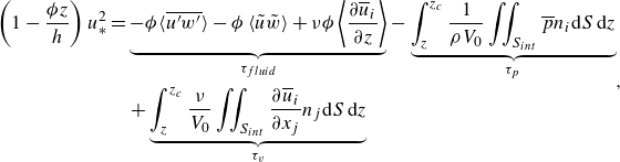 \begin{equation} \begin{aligned} \left(1 - \frac {\phi z}{h}\right) u_*^2 &= \underbrace {-\phi \langle \overline {u^{\prime}w^{\prime}}\rangle - \phi \left \langle \tilde {u} \tilde {w}\right \rangle + \nu \phi \left \langle \frac {\partial \overline {u}_i}{\partial z} \right \rangle }_{\tau _{{fluid}}} - \underbrace {\int _{z}^{z_c} \frac {1}{\rho V_0} \iint _{S_{{int}}} \overline {p} n_i {\rm d}S \, {\rm d}z}_{\tau _p} \\ &\quad +\underbrace {\int _{z}^{z_c} \frac {\nu }{V_0} \iint _{S_{{int}}} \frac {\partial \overline {u}_i}{\partial x_j} n_j {\rm d}S \, {\rm d}z}_{\tau _v} \end{aligned}, \end{equation}
where $z_c$
corresponds to the top of the interfacial sublayer (i.e. crest of the roughness elements),
$z_c$
corresponds to the top of the interfacial sublayer (i.e. crest of the roughness elements), $S_{int}$
is the water–sediment interface and
$S_{int}$
is the water–sediment interface and $n_i$
is the unit vector normal to the bed surface pointing into the fluid. The shear-stress balance includes turbulent
$n_i$
is the unit vector normal to the bed surface pointing into the fluid. The shear-stress balance includes turbulent $\langle \overline {u^{\prime}w^{\prime}}\rangle$
, form-induced
$\langle \overline {u^{\prime}w^{\prime}}\rangle$
, form-induced $\left \langle \tilde {u} \tilde {w}\right \rangle$
and viscous stresses
$\left \langle \tilde {u} \tilde {w}\right \rangle$
and viscous stresses $\left \langle {\partial \overline {u}_i}/{\partial z} \right \rangle$
, which together correspond to the total fluid stress
$\left \langle {\partial \overline {u}_i}/{\partial z} \right \rangle$
, which together correspond to the total fluid stress $\tau _{{fluid}}$
, and pressure
$\tau _{{fluid}}$
, and pressure $\tau _{p}$
and viscous drag
$\tau _{p}$
and viscous drag $\tau _{v}$
, which are a sink of momentum caused by the roughness elements. The form-induced stress term is also the covariance of spatial velocity fluctuations. The last two terms in the right-hand part are zero above the roughness elements.
$\tau _{v}$
, which are a sink of momentum caused by the roughness elements. The form-induced stress term is also the covariance of spatial velocity fluctuations. The last two terms in the right-hand part are zero above the roughness elements.
4.2. Double-averaged kinetic energy budget
The total kinetic energy is now composed by the mean (MKE), turbulent (TKE) and form-induced or dispersive (DKE) contributions
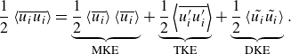 \begin{equation} \frac {1}{2}\left \langle \overline {u_i u_i} \right \rangle = \underbrace {\frac {1}{2} \left \langle \overline {u_i} \right \rangle \left \langle \overline {u_i} \right \rangle }_{\text{MKE}} + \underbrace {\frac {1}{2} \left \langle \overline {u^{\prime}_i u^{\prime}_i} \right \rangle }_{\text{TKE}} + \underbrace {\frac {1}{2}\left \langle \tilde {u_i} \tilde {u_i} \right \rangle }_{\text{DKE}}. \end{equation}
Papadopoulos et al. (Reference Papadopoulos, Nikora, Cameron, Stewart and Gibbins2020) derived the kinetic energy budgets for open-channel flows with rough beds using the intrinsic average and the porosity function. For a fixed bed and a double-averaged steady and uniform flow in the streamwise and spanwise directions, the energy conservation equations for MKE, DKE and TKE are simplified as follows respectively (see Papadopoulos et al. Reference Papadopoulos, Nikora, Cameron, Stewart and Gibbins2020 for details):
 \begin{align} 0 &= \underbrace {\phi \left \langle \overline {u}\right \rangle gS_b}_{S_g} + \underbrace {\phi \langle \overline {u^{\prime}w^{\prime}}\rangle \frac {\partial \left \langle \overline {u}\right \rangle }{\partial z}}_{I_{TM}} + \underbrace {\phi \left \langle \tilde {u} \tilde {w}\right \rangle \frac {\partial \left \langle \overline {u}\right \rangle }{\partial z}}_{I_{DM}} + \underbrace {\frac {\left \langle \overline {u}\right \rangle }{\rho V_0} \iint _{S_{{int}}} \overline {p} n_1 {\rm d} S}_{I_p} \nonumber\\ &\quad - \underbrace {\frac {\nu \left \langle \overline {u}\right \rangle }{V_0} \iint _{S_{{int}}} \frac {\partial \overline {u}}{\partial x_j} n_j {\rm d} S}_{I_{v}} - \underbrace {\frac {\partial \phi \langle \overline {u^{\prime}w^{\prime}}\rangle \left \langle \overline {u}\right \rangle }{\partial z}}_{TM_{T}} - \underbrace {\frac {\partial \phi \left \langle \tilde {u}\tilde {w}\right \rangle \left \langle \overline {u}\right \rangle }{\partial z}}_{TM_{D}} \nonumber\\ &\quad + \underbrace {\nu \frac {\partial }{\partial z} \left (\left \langle \overline {u}\right \rangle \frac {\partial \phi \left \langle \overline {u}\right \rangle }{\partial z} \right )}_{TM_{v}} - \underbrace {\phi \nu \frac {\partial \left \langle \overline {u}\right \rangle }{\partial z} \frac {\partial \left \langle \overline {u}\right \rangle }{\partial z}}_{\epsilon _{MM}} - \underbrace {\phi \nu \left \langle \frac {\partial \tilde {u}}{\partial z} \right \rangle \frac {\partial \left \langle \overline {u}\right \rangle }{\partial z}}_{\epsilon _{MD}}, \end{align}
 \begin{align} 0 &= -\underbrace {\phi \langle \tilde {u}\tilde {w} \rangle \frac {\partial \langle \overline {u} \rangle }{\partial z}}_{I_{DM}} + \underbrace {\phi \left \langle \overline {u^{\prime}_iu^{\prime}_j} \frac {\partial \tilde {u}_{i}}{\partial x_j} \right \rangle }_{I_{TD}} - \underbrace {\frac {\langle \overline {u} \rangle }{\rho V_0} \iint _{S_{int}} \overline {p} n_1 {\rm d}S}_{I_p} + \underbrace {\frac {\nu \langle \overline {u} \rangle }{V_0} \iint _{S_{int}} \frac {\partial \overline {u}}{\partial x_{j}} n_j {\rm d}S}_{I_v} \nonumber\\ &\quad - \underbrace {\frac {1}{2} \frac {\partial \phi \left \langle \tilde {u}_i \tilde {u}_{i}\tilde {w}\right \rangle }{\partial z}}_{TD_{D}} - \underbrace { \frac {\partial \phi \left \langle \tilde {u}_i \overline {u^{\prime}_iw^{\prime}}\right \rangle }{\partial z}}_{TD_{T}} - \underbrace {\frac {1}{\rho } \frac {\partial \phi \left \langle \tilde {p} \tilde {w}\right \rangle }{\partial z}}_{TD_{p}} + \underbrace {\nu \frac {\partial }{\partial z} \left ( \phi \left \langle \tilde {u}_{i} \frac {\partial \tilde {u_{i}}}{\partial z} \right \rangle \right )}_{TD_{v}} \nonumber\\ &\quad - \underbrace {\phi \nu \left \langle \frac {\partial \tilde {u}}{\partial z} \right \rangle \frac {\partial \left \langle \overline {u}\right \rangle }{\partial z}}_{\epsilon _{MD}} - \underbrace {\phi \nu \left \langle \frac {\partial \tilde {u}_{i}}{\partial x_{j}} \frac { \partial \tilde {u}_{i}}{\partial x_{j}} \right \rangle }_{\epsilon _{DD}}, \end{align}
 \begin{align} 0 &= -\underbrace {\phi \langle \overline {u^{\prime}w^{\prime}}\rangle \frac {\partial \left \langle \overline {u}\right \rangle }{\partial z}}_{I_{TM}} - \underbrace {\phi \left \langle \overline {u^{\prime}_iu^{\prime}_j} \frac {\partial \tilde {u_i}}{\partial x_j} \right \rangle }_{I_{TD}} - \underbrace {\frac {1}{2} \frac {\partial \phi \left \langle \overline {u^{\prime}_iu^{\prime}_i} \tilde {w}\right \rangle }{\partial z}}_{TT_{D}} - \underbrace {\frac {1}{2} \frac {\partial \phi \left \langle \overline {u^{\prime}_iu^{\prime}_iw^{\prime}}\right \rangle }{\partial z}}_{TT_{T}} \nonumber\\ &\quad - \underbrace {\frac {1}{\rho } \frac {\partial \phi \langle \overline {p^{\prime}w^{\prime}}\rangle }{\partial z}}_{TT_{p}} + \underbrace {\frac {1}{2} \nu \frac {\partial }{\partial z} \left ( \frac {\partial \phi \langle \overline {u^{\prime}_iu^{\prime}_i}\rangle }{\partial z} \right )}_{TT_{v}} - \underbrace {\phi \nu \left \langle \overline {\frac {\partial u^{\prime}_i}{\partial x_j} \frac {\partial u^{\prime}_i}{\partial x_j}} \right \rangle }_{\epsilon _{TT}} .\end{align}
The energy is injected into the mean flow by the potential energy coming from gravity ( $S_g$
). Part of this energy is transferred to the turbulent and form-induced fields by the work done by turbulent and form-induced stresses against the mean flow (
$S_g$
). Part of this energy is transferred to the turbulent and form-induced fields by the work done by turbulent and form-induced stresses against the mean flow ( $I_{TM}$
and
$I_{TM}$
and $I_{DM}$
, respectively). These terms are usually negative, and therefore represent a sink of MKE and a gain of TKE and DKE. Term
$I_{DM}$
, respectively). These terms are usually negative, and therefore represent a sink of MKE and a gain of TKE and DKE. Term $I_{TD}$
corresponds to the kinetic energy transferred from the form-induced flow to the turbulent field (usually negative and hence a gain of TKE and a loss of DKE). Energy coming from viscous (
$I_{TD}$
corresponds to the kinetic energy transferred from the form-induced flow to the turbulent field (usually negative and hence a gain of TKE and a loss of DKE). Energy coming from viscous ( $I_v$
), and pressure (
$I_v$
), and pressure ( $I_p$
) drag constitute a loss of MKE and a gain of DKE. Terms
$I_p$
) drag constitute a loss of MKE and a gain of DKE. Terms $I_{TM}$
,
$I_{TM}$
, $I_{DM}$
,
$I_{DM}$
, $I_{TD}$
,
$I_{TD}$
, $I_v$
and
$I_v$
and $I_p$
, are then inter-budget exchanges between MKE, TKE and DKE. The following terms in the equations correspond to transport of kinetic energy by turbulence:
$I_p$
, are then inter-budget exchanges between MKE, TKE and DKE. The following terms in the equations correspond to transport of kinetic energy by turbulence: $TM_T$
(of MKE),
$TM_T$
(of MKE), $TT_T$
(of TKE) and
$TT_T$
(of TKE) and $TD_T$
(of DKE); form-induced stresses
$TD_T$
(of DKE); form-induced stresses $TM_D$
(of MKE),
$TM_D$
(of MKE), $TT_D$
(of TKE) and
$TT_D$
(of TKE) and $TD_D$
(of DKE); pressure
$TD_D$
(of DKE); pressure $TT_p$
(of TKE) and
$TT_p$
(of TKE) and $TD_p$
(of DKE); and viscosity
$TD_p$
(of DKE); and viscosity $TM_v$
(of MKE),
$TM_v$
(of MKE), $TT_v$
(of TKE) and
$TT_v$
(of TKE) and $TD_v$
(of DKE). Finally, energy is dissipated into heat by viscosity through
$TD_v$
(of DKE). Finally, energy is dissipated into heat by viscosity through $\epsilon _{MM}$
,
$\epsilon _{MM}$
, $\epsilon _{MD}$
,
$\epsilon _{MD}$
, $\epsilon _{TT}$
and
$\epsilon _{TT}$
and $\epsilon _{DD}$
.
$\epsilon _{DD}$
.
5. Double-averaged momentum conservation equation
5.1. Double-averaged velocity
To apply the double-averaging procedure, the intrinsic averaging is performed over thin slabs covering the entire horizontal area and the grid spacing $\Delta z$
. A large slab is needed to include all spatial disturbances of the time-averaged quantities and therefore reach a steady and statistically 1-D flow, with velocity statistics depending only on z. We checked that this is achieved as
$\Delta z$
. A large slab is needed to include all spatial disturbances of the time-averaged quantities and therefore reach a steady and statistically 1-D flow, with velocity statistics depending only on z. We checked that this is achieved as $\left \langle \overline {v}\right \rangle$
,
$\left \langle \overline {v}\right \rangle$
, $\left \langle \overline {w} \right \rangle$
,
$\left \langle \overline {w} \right \rangle$
, $\langle \overline {u^{\prime}v^{\prime}}\rangle$
and
$\langle \overline {u^{\prime}v^{\prime}}\rangle$
and $\langle \overline {v^{\prime}w^{\prime}}\rangle$
are almost zero along the entire water depth, for the chosen spatial-averaging slabs.
$\langle \overline {v^{\prime}w^{\prime}}\rangle$
are almost zero along the entire water depth, for the chosen spatial-averaging slabs.
The averaged velocity profile and velocity gradient along the vertical coordinate are depicted in figure 10. As observed previously (Dey & Das Reference Dey and Das2012; Sarkar et al. Reference Sarkar, Papanicolaou and Dey2016), it presents the typical shape of flows over rough beds and obstacles, with a velocity deficit and inflection points above the boulders and at the top of the rough bed resulting from the shear layer generated by the obstacles. Within the rough bed, near the trough of the hemispheres, the velocity becomes slightly negative as already observed by Pokrajac, McEwan & Nikora (Reference Pokrajac, McEwan and Nikora2008) in the case of ‘d-type’ roughness elements.
(a) Double-averaged velocity profile where the inset corresponds to the porosity function around the rough bed (zero is the crest of the hemispheres). (b) Double-averaged velocity gradient where the red dashed line shows a constant value obtained around the boulders. The dashed horizontal lines in (a) and (b) correspond to the top of the rough bed (rb) and the top of the boulders (B).
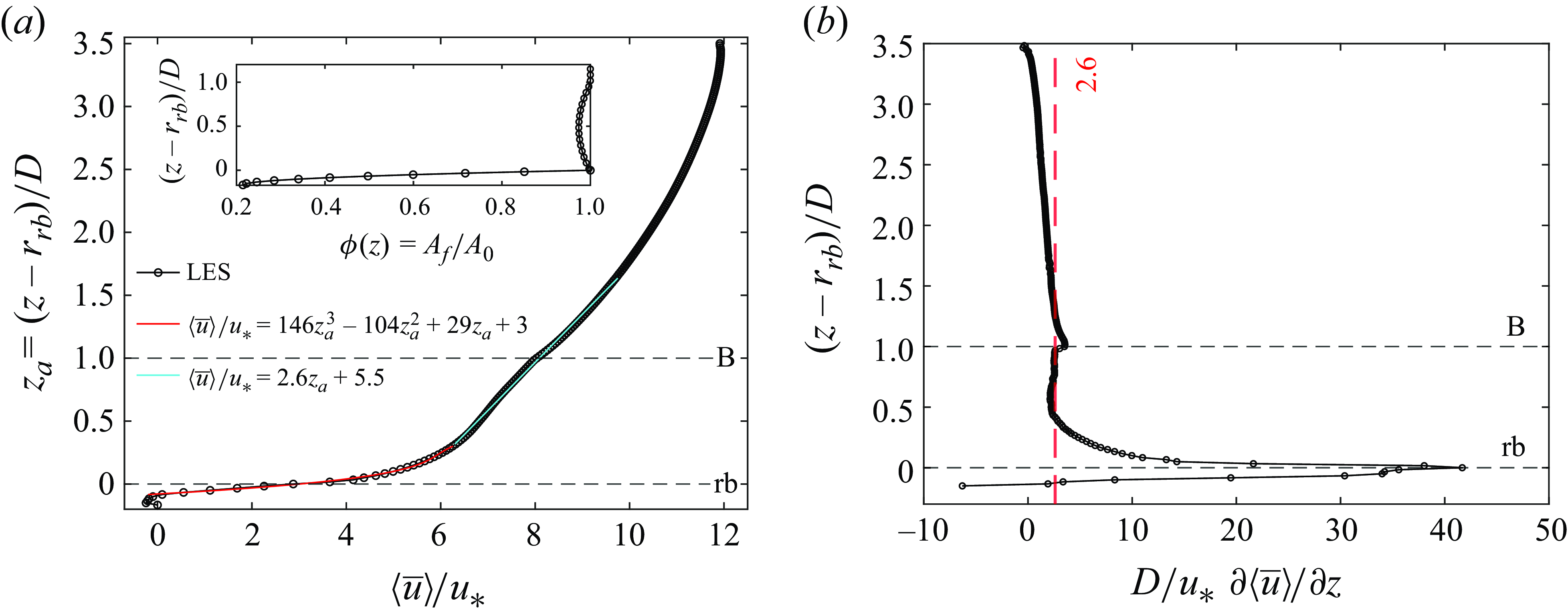
The vertical variations in the velocity profile are influenced by dynamic processes within the water column, which depend on the roughness characteristics and bed configuration. While the velocity profile above the rough bed appears to be linear, the velocity gradient shown in figure 10(b) reveals a more complex structure. The gradient exhibits a second-degree polynomial shape, indicating that the velocity profile in this region follows a third-degree polynomial. Within the boulder layer, the velocity profile transitions to a linear behaviour, characterised by a constant velocity gradient (red line in figure 10 b). These findings align with the observations of Sarkar et al. (Reference Sarkar, Papanicolaou and Dey2016) for gravel beds with large gravel obstacles.
In the flow over a rough bed with macroroughness elements the universal log law may be present depending mainly on the flow relative submergence. The logarithmic velocity profile is produced above the form-induced sublayer (Nikora et al. Reference Nikora, Goring, McEwan and Griffiths2001), which in fully rough conditions is expressed as follows (White & Majdalani Reference White and Majdalani2006):
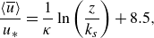 \begin{equation} \frac {\left \langle \overline {u} \right \rangle }{u_*} = \frac {1}{\kappa } \ln \left ( \frac {z}{k_s} \right ) + 8.5 ,\end{equation}
where $\kappa = 0.41$
is the von Kármán constant and
$\kappa = 0.41$
is the von Kármán constant and $k_s$
is the effective roughness height obtained by fitting the log law to the velocity profile, as shown in figure 11, where a value of
$k_s$
is the effective roughness height obtained by fitting the log law to the velocity profile, as shown in figure 11, where a value of $k_{s-dat} = 0.9D$
is obtained. It is not straightforward to estimate
$k_{s-dat} = 0.9D$
is obtained. It is not straightforward to estimate $k_s$
when no information of the velocity profile is available, especially in the case of multi-scale roughness. Huang et al. (Reference Huang, Simoëns, Vinkovic, Le Ribault, Dupont and Bergametti2016) suggested the use of a fraction of the roughness length based on the roughness density parameter depending on the flow regime: isolated, wake interfering or skimming, without considering multi-scale roughness conditions. Recently Meneveau et al. (Reference Meneveau, Hutchins and Chung2024) formulated a novel method to estimate
$k_s$
when no information of the velocity profile is available, especially in the case of multi-scale roughness. Huang et al. (Reference Huang, Simoëns, Vinkovic, Le Ribault, Dupont and Bergametti2016) suggested the use of a fraction of the roughness length based on the roughness density parameter depending on the flow regime: isolated, wake interfering or skimming, without considering multi-scale roughness conditions. Recently Meneveau et al. (Reference Meneveau, Hutchins and Chung2024) formulated a novel method to estimate $k_s$
based solely on geometric surface information of the rough bed elevation
$k_s$
based solely on geometric surface information of the rough bed elevation $h_b(x,y)$
. The method approximates the total drag
$h_b(x,y)$
. The method approximates the total drag $f_x$
generated on the rough surface using the local slope
$f_x$
generated on the rough surface using the local slope ${\partial h_b}/{\partial x}$
, a sheltering function
${\partial h_b}/{\partial x}$
, a sheltering function $F^{sh} (x,y;\theta )$
, and the potential flow over a ramp at an angle
$F^{sh} (x,y;\theta )$
, and the potential flow over a ramp at an angle $\alpha$
to estimate the velocity
$\alpha$
to estimate the velocity $U_k$
at height
$U_k$
at height $z_k$
. Their equations are written as follows:
$z_k$
. Their equations are written as follows:
 \begin{equation} f_x = u_*^2 A = U_k \mathcal{W}_L, \end{equation}
(a) Logarithmic law of the wall for fully rough conditions shown in (5.1) fitted to the double-averaged velocity data computed from the LES where $k_{s-dat}=0.9D$
is obtained. (b) Comparison of velocity profiles obtained from LES, the one fitted from (5.1) with
$k_{s-dat}=0.9D$
is obtained. (b) Comparison of velocity profiles obtained from LES, the one fitted from (5.1) with $k_{s-dat}$
and the one using
$k_{s-dat}$
and the one using $k_{s-mod}$
computed from the method of Meneveau et al. (Reference Meneveau, Hutchins and Chung2024).
$k_{s-mod}$
computed from the method of Meneveau et al. (Reference Meneveau, Hutchins and Chung2024).
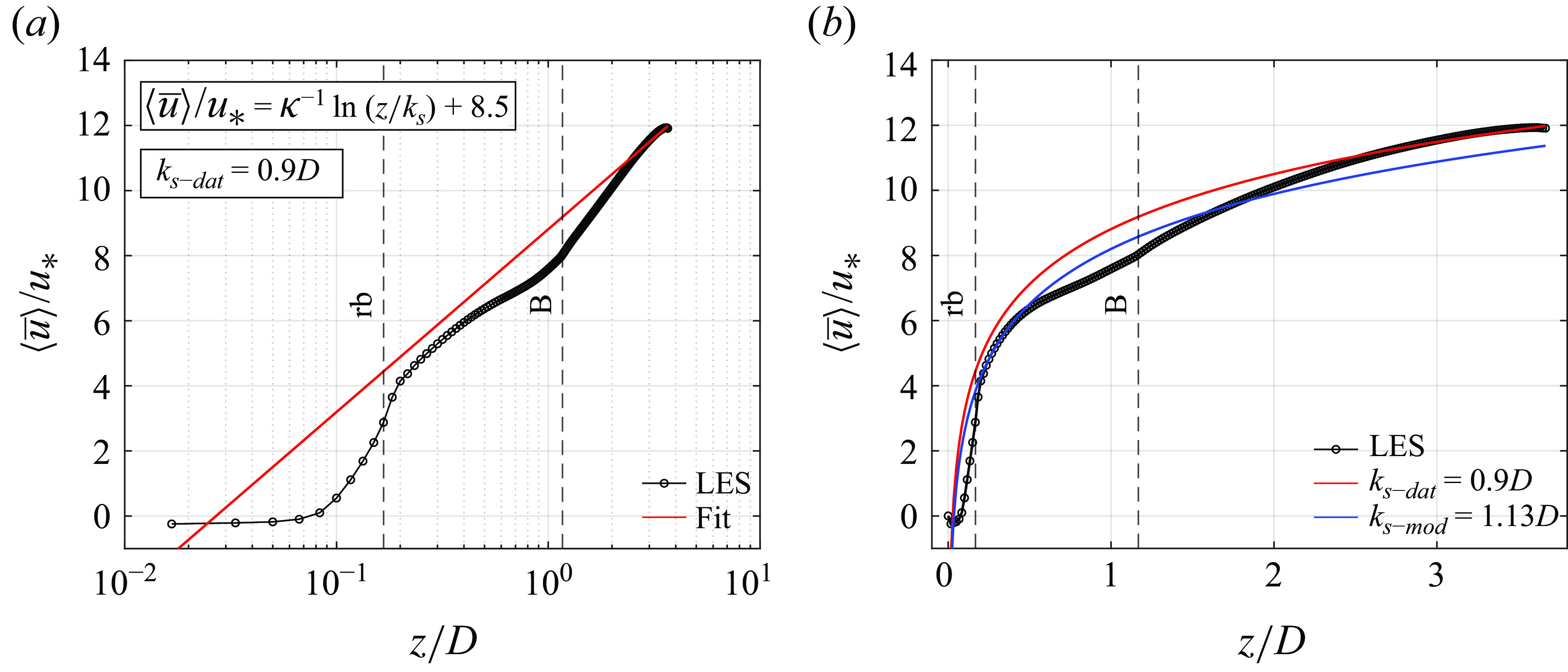
where $\mathcal{W}_L$
is the wind-shade factor in the longitudinal direction, expressed as
$\mathcal{W}_L$
is the wind-shade factor in the longitudinal direction, expressed as
 \begin{equation} \mathcal{W}_L = \left \lt \hat {n}^2_x(x,y) \frac {\alpha }{\pi + \alpha } \frac {\partial h_b}{\partial x} F^{sh} (x,y;\theta ) \right \gt _{x,y}, \end{equation}
where $\alpha = \text{arctan}|\nabla _{h} h_b (x,y)|$
and
$\alpha = \text{arctan}|\nabla _{h} h_b (x,y)|$
and $F^{sh} = H (\theta - \beta (x,y))$
, where
$F^{sh} = H (\theta - \beta (x,y))$
, where $\nabla _{h}=\partial _xi +\partial _yj$
,
$\nabla _{h}=\partial _xi +\partial _yj$
, $H(x)$
is the Heaviside function and
$H(x)$
is the Heaviside function and $\beta$
is the backward horizon angle only depending on the surface geometry. Then
$\beta$
is the backward horizon angle only depending on the surface geometry. Then $U_k = 1/\sqrt {\mathcal{W}_L}$
and
$U_k = 1/\sqrt {\mathcal{W}_L}$
and $k_s$
can be estimated based on (5.1) for
$k_s$
can be estimated based on (5.1) for $U_k$
at
$U_k$
at $z_k = a_p k^{\prime}_p$
, where
$z_k = a_p k^{\prime}_p$
, where $k^{\prime}_p$
is estimated with a ramp function. The turbulence spreading angle
$k^{\prime}_p$
is estimated with a ramp function. The turbulence spreading angle $\theta = 10$
degrees and
$\theta = 10$
degrees and $a_p = 3$
were established as suggested by Meneveau et al. (Reference Meneveau, Hutchins and Chung2024) as the values that gave the highest correlation between
$a_p = 3$
were established as suggested by Meneveau et al. (Reference Meneveau, Hutchins and Chung2024) as the values that gave the highest correlation between $k_{s-dat}$
and
$k_{s-dat}$
and $k_{s-mod}$
. Then,
$k_{s-mod}$
. Then, $k_{s-mod}$
can be computed from (5.1) as
$k_{s-mod}$
can be computed from (5.1) as
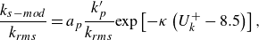 \begin{equation} \frac {k_{s-mod}}{k_{rms}} = a_p \frac {k^{\prime}_p}{k_{rms}} \text{exp}\left[-\kappa \left(U_k^+ - 8.5\right)\right] ,\end{equation}
where $k_{rms} = \langle (h_b - \overline {k})^2\rangle ^{1/2}$
and
$k_{rms} = \langle (h_b - \overline {k})^2\rangle ^{1/2}$
and $\overline {k} = \langle h_b \rangle$
. This method can be applied to multiple rough bed configurations with the only limitation of having a single-valued function of
$\overline {k} = \langle h_b \rangle$
. This method can be applied to multiple rough bed configurations with the only limitation of having a single-valued function of $h$
at each point
$h$
at each point $(x,y)$
in the horizontal plane. Therefore, since this is not true for spheres, the geometry of the lower part of the boulders is slightly modified. The value of
$(x,y)$
in the horizontal plane. Therefore, since this is not true for spheres, the geometry of the lower part of the boulders is slightly modified. The value of $k_{s-mod}$
is estimated based on the surface roughness geometry
$k_{s-mod}$
is estimated based on the surface roughness geometry $h_b(x,y)$
used in the present study and compared with the value obtained by fitting the log law of (5.1) to the LES data (
$h_b(x,y)$
used in the present study and compared with the value obtained by fitting the log law of (5.1) to the LES data ( $k_{s-dat}$
, figure 11
a). A value of
$k_{s-dat}$
, figure 11
a). A value of $k_{s-mod} = 1.13D$
is obtained (figure 11
b), which agrees well with the observed value
$k_{s-mod} = 1.13D$
is obtained (figure 11
b), which agrees well with the observed value $k_{s-dat} = 0.9D$
. The ratios
$k_{s-dat} = 0.9D$
. The ratios $k_{s-mod}/k_{s-dat} = 1.25$
and
$k_{s-mod}/k_{s-dat} = 1.25$
and $k_{s-dat}/k_{rms}=5.9$
are in good agreement with the majority of the values observed by Meneveau et al. (Reference Meneveau, Hutchins and Chung2024) when evaluating the performance of their model. As they indicate, in the presence of a few large-scale and many small-scale elements, the method can result in an over-prediction of the drag. Therefore, the authors proposed the use of a
$k_{s-dat}/k_{rms}=5.9$
are in good agreement with the majority of the values observed by Meneveau et al. (Reference Meneveau, Hutchins and Chung2024) when evaluating the performance of their model. As they indicate, in the presence of a few large-scale and many small-scale elements, the method can result in an over-prediction of the drag. Therefore, the authors proposed the use of a $1/7$
velocity power law impinging on the roughness elements. However, with this correction a slightly worse agreement between
$1/7$
velocity power law impinging on the roughness elements. However, with this correction a slightly worse agreement between $k_{s-mod}$
and
$k_{s-mod}$
and $k_{s-dat}$
is obtained resulting in an under-prediction of the expected value
$k_{s-dat}$
is obtained resulting in an under-prediction of the expected value $k_{s-mod}/k_{s-dat} = 0.43$
.
$k_{s-mod}/k_{s-dat} = 0.43$
.
As illustrated in figure 11(a), logarithmic profile only exists in the upper layer, within a small fraction of the water depth corresponding to $(z-r_{rb})/D$
between 2.5 and 3.5. This agrees with the findings of Sarkar et al. (Reference Sarkar, Papanicolaou and Dey2016). Figure 11 shows that
$(z-r_{rb})/D$
between 2.5 and 3.5. This agrees with the findings of Sarkar et al. (Reference Sarkar, Papanicolaou and Dey2016). Figure 11 shows that $k_s$
is relatively well predicted by the method of Meneveau et al. (Reference Meneveau, Hutchins and Chung2024). However, it is important to note that this parameterisation was developed to characterise drag based solely on surface roughness geometry, or an equivalent roughness length (
$k_s$
is relatively well predicted by the method of Meneveau et al. (Reference Meneveau, Hutchins and Chung2024). However, it is important to note that this parameterisation was developed to characterise drag based solely on surface roughness geometry, or an equivalent roughness length ( $k_s$
or
$k_s$
or $z_0$
), and it does not imply the presence of a universal log-law profile. In the low relative submergence conditions of the present study, the emergence of a fully developed log layer is unlikely. For instance, Jiménez (Reference Jiménez2004) suggested that a true log law requires the flow depth to be at least 40 times the roughness scale, which is much larger than in our configuration.
$z_0$
), and it does not imply the presence of a universal log-law profile. In the low relative submergence conditions of the present study, the emergence of a fully developed log layer is unlikely. For instance, Jiménez (Reference Jiménez2004) suggested that a true log law requires the flow depth to be at least 40 times the roughness scale, which is much larger than in our configuration.
5.2. Double-averaged shear-stress contributions
To evaluate the different terms of the total shear stress in the water column as given by (4.1), in figure 12 we show the vertical profiles of the contribution of each term. At the top of the hemispheres, the total fluid stress corresponds to approximately half of the total bed shear stress, which is an integral of pressure and viscous drag terms due to both the rough bed and the boulders. Red and blue lines in figure 12 show that the actual force acting on the hemispheres is half the total drag (or bed shears stress which is due to both boulders and hemispheres). This observation has important implications for sediment transport as it demonstrates the power of the double-averaging approach for isolating part of the total drag which is directly relevant for bed particle mobilisation.
Profiles of the different contributions to the total shear stress depicted with a black line. Different stresses shown with points correspond to turbulent (black), form-induced (grey), total fluid stresses (red) and total drag (blue). Viscous stress is depicted with a black dashed line. Total fluid stresses correspond to the sum of turbulent and form-induced contributions (viscous stresses are negligible). The inset corresponds to a zoom around the top of the rough bed. Total drag depicted in blue is computed as a residual of equation (4.1).
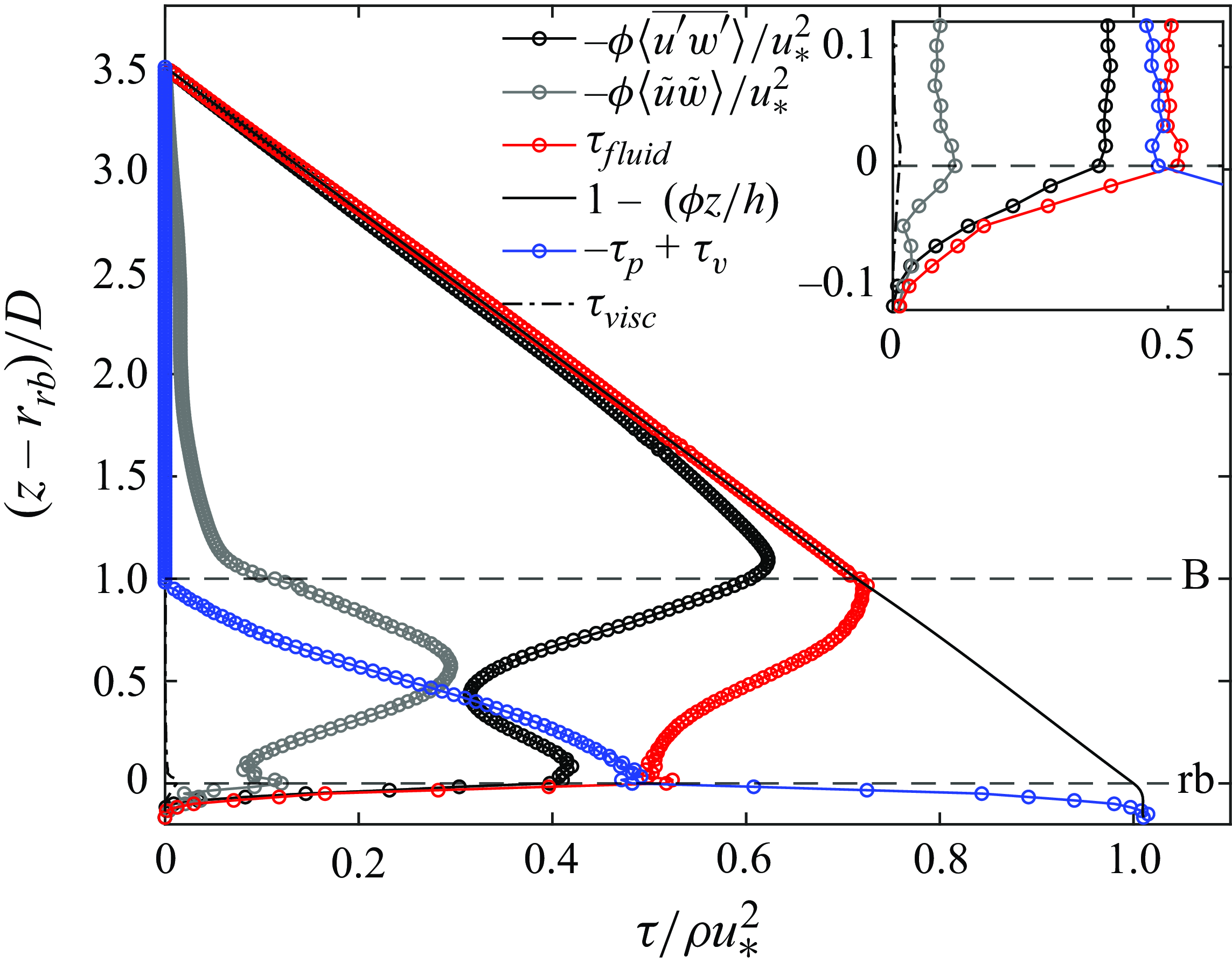
Local peaks of turbulent and form-induced stresses appear at the top of the roughness elements, and global peaks of turbulent and form-induced stresses are produced at the top and centre of the boulders, respectively. The peak of turbulent stress agrees with previous experimental observations in gravel beds, related to the production of TKE in the shear layer generated at the top of the roughness elements of the bed, as shown in figure 5 (Mignot et al. Reference Mignot, Hurther and Barthélemy2009; Sarkar & Dey Reference Sarkar and Dey2010; Dey & Das Reference Dey and Das2012). Within the boulder region, an increase in Reynolds stress partially compensates with a decrease in form-induced stress, which agrees with the previous findings of Zampiron et al. (Reference Zampiron, Cameron and Nikora2021) in the flow over triangular-shaped ridges.
Form-induced stresses and total drag generated by the boulders and rough bed significantly affect a considerable portion of the water column. The drag caused by the roughness elements creates an inflection point in the fluid stress profile at the boulder tops (red curve in figure 12), where shear stress increases above this point and decreases below it.
In figure 13 we show the relative magnitude of the form-induced stress to turbulent stress, and to the total shear-stress distribution. Form-induced stress is comparable to the turbulent stress in the region within the boulders. Below the top of the rough bed this ratio has a higher uncertainty due to the low values of Reynolds stresses resulting from an attenuation of turbulence within the rough bed. In the boulder region, the form-induced to turbulent-stress ratio monotonically increases from slightly above the top of the rough bed to the middle of the boulders, reaching a peak where form-induced stresses almost equal turbulent ones ( $\langle \tilde {u}\tilde {w}\rangle / \overline {u^{\prime}w^{\prime}} \approx 0.9$
at the location of the global peak of form-induced stress). Then this ratio decreases toward the top of the boulders, where the turbulent stress reaches its global peak. In the rest of the water column, these ratios are small and relatively constant.
$\langle \tilde {u}\tilde {w}\rangle / \overline {u^{\prime}w^{\prime}} \approx 0.9$
at the location of the global peak of form-induced stress). Then this ratio decreases toward the top of the boulders, where the turbulent stress reaches its global peak. In the rest of the water column, these ratios are small and relatively constant.
Ratio between form-induced stresses and (a) turbulent stresses, and (b) total shear-stress distribution.
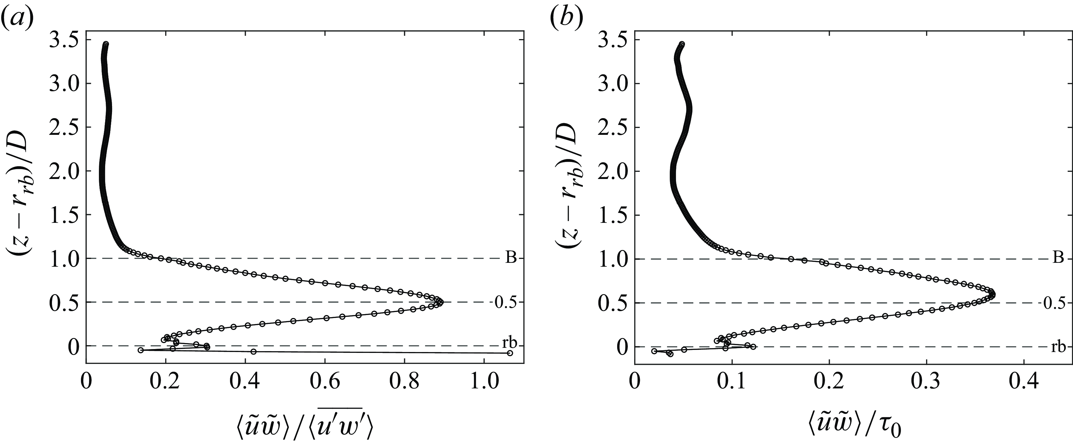
The peak stress ratio is generally higher than previously reported values for rough beds with varying roughness shapes, configurations and relative submergence (Mignot et al. Reference Mignot, Hurther and Barthélemy2009; Sarkar & Dey Reference Sarkar and Dey2010; Dey & Das Reference Dey and Das2012; Sarkar et al. Reference Sarkar, Papanicolaou and Dey2016). This is primarily due to the low relative submergence and large boulder spacing used here, which allows wakes to develop freely, causing significant spatial variations within the averaging volume. Another contributing factor is the influence of the SCs depicted in figure 4, as will be shown and discussed in § 5.3. In the boulder layer, the form-induced stress exhibits a large contribution to the total shear-stress distribution ( $\langle \tilde {u}\tilde {w}\rangle / \tau$
), reaching a peak of approximately 0.37 slightly above mid-boulder elevation (figure 13
b).
$\langle \tilde {u}\tilde {w}\rangle / \tau$
), reaching a peak of approximately 0.37 slightly above mid-boulder elevation (figure 13
b).
The ratio of maximum form-induced stress to bed shear stress ( $\left \langle \tilde {u} \tilde {w}\right \rangle / u_*^2 \approx 0.3$
) aligns with the range observed for SCs (0.25–0.3) over triangular and rectangular ridges (Vanderwel et al. Reference Vanderwel, Stroh, Kriegseis, Frohnapfel and Ganapathisubramani2019; Zampiron et al. Reference Zampiron, Cameron and Nikora2021). Unlike other geometries such as rectangles or sharp-edged vertical surfaces, where maximum form-induced stresses typically occur near the roughness tops (Pokrajac et al. Reference Pokrajac, Campbell, Nikora, Manes and McEwan2007; Rouzes et al. Reference Rouzes, Moulin, Florens and Eiff2019), the peak here is shifted due to differences in geometry. Sharp-edged elements enhance the formation of the shear layer, leading to wider wakes and more extensive vertical recirculation compared with spherical obstacles. Within the rough bed, the contribution of form-induced stresses to total shear stress is relatively minor, partly explained by the lower values of total fluid stress compared with total drag.
$\left \langle \tilde {u} \tilde {w}\right \rangle / u_*^2 \approx 0.3$
) aligns with the range observed for SCs (0.25–0.3) over triangular and rectangular ridges (Vanderwel et al. Reference Vanderwel, Stroh, Kriegseis, Frohnapfel and Ganapathisubramani2019; Zampiron et al. Reference Zampiron, Cameron and Nikora2021). Unlike other geometries such as rectangles or sharp-edged vertical surfaces, where maximum form-induced stresses typically occur near the roughness tops (Pokrajac et al. Reference Pokrajac, Campbell, Nikora, Manes and McEwan2007; Rouzes et al. Reference Rouzes, Moulin, Florens and Eiff2019), the peak here is shifted due to differences in geometry. Sharp-edged elements enhance the formation of the shear layer, leading to wider wakes and more extensive vertical recirculation compared with spherical obstacles. Within the rough bed, the contribution of form-induced stresses to total shear stress is relatively minor, partly explained by the lower values of total fluid stress compared with total drag.
5.3. Quadrant contribution to form-induced stresses
The DAM analysis can also provide additional insights into the different contributions to form-induced stresses. Conditional statistics based on the quadrant analysis proposed by Pokrajac et al. (Reference Pokrajac, Campbell, Nikora, Manes and McEwan2007) consider the spatial fluctuations of the time-averaged streamwise and vertical velocities in analogy to the quadrant analysis used for Reynolds shear stress, as presented in § 3.4 and in figure 9. Using this methodology we study the different contributions to the profile of form-induced stresses depicted in figure 12, based on the sign of $\tilde {u}$
and
$\tilde {u}$
and $\tilde {w}$
resulting on four quadrants which are Q1 (
$\tilde {w}$
resulting on four quadrants which are Q1 ( $\tilde {u}\gt 0,\tilde {w}\gt 0$
), Q2 (
$\tilde {u}\gt 0,\tilde {w}\gt 0$
), Q2 ( $\tilde {u}\lt 0,\tilde {w}\gt 0$
), Q3 (
$\tilde {u}\lt 0,\tilde {w}\gt 0$
), Q3 ( $\tilde {u}\lt 0,\tilde {w}\lt 0$
) and Q4 (
$\tilde {u}\lt 0,\tilde {w}\lt 0$
) and Q4 ( $\tilde {u}\gt 0,\tilde {w}\lt 0$
). The procedure consists of the following steps: (i) computing
$\tilde {u}\gt 0,\tilde {w}\lt 0$
). The procedure consists of the following steps: (i) computing $\tilde {u}$
and
$\tilde {u}$
and $\tilde {w}$
by subtracting the spatial mean to local time-averaged velocities (
$\tilde {w}$
by subtracting the spatial mean to local time-averaged velocities ( $\overline {u}$
and
$\overline {u}$
and $\overline {w}$
). (ii) At each averaging volume, separating the values of
$\overline {w}$
). (ii) At each averaging volume, separating the values of $\tilde {u}\tilde {w}$
according to the four quadrants. (iii) Then, averaging
$\tilde {u}\tilde {w}$
according to the four quadrants. (iii) Then, averaging $\tilde {u}\tilde {w}$
separately for each quadrant to calculate the mean magnitude, and computing the relative frequency (number of points of each quadrant with respect to the entire fluid volume). (iv) Finally, the contribution of each quadrant to the form-induced stress at each depth is obtained as the product of the average magnitude and the relative frequency. Profiles of the different quadrant contributions to the form-induced stress are shown in figure 14 as a function of
$\tilde {u}\tilde {w}$
separately for each quadrant to calculate the mean magnitude, and computing the relative frequency (number of points of each quadrant with respect to the entire fluid volume). (iv) Finally, the contribution of each quadrant to the form-induced stress at each depth is obtained as the product of the average magnitude and the relative frequency. Profiles of the different quadrant contributions to the form-induced stress are shown in figure 14 as a function of $z$
. The sum of all contributions of figure 14(a) is equal to the form-induced stress, as depicted in figure 12.
$z$
. The sum of all contributions of figure 14(a) is equal to the form-induced stress, as depicted in figure 12.
Profiles of the different contribution to form-induced stress. The different quadrants correspond to Q1: ( $\tilde {u}\gt 0,\tilde {w}\gt 0$
), Q2: (
$\tilde {u}\gt 0,\tilde {w}\gt 0$
), Q2: ( $\tilde {u}\lt 0,\tilde {w}\gt 0$
), Q3: (
$\tilde {u}\lt 0,\tilde {w}\gt 0$
), Q3: ( $\tilde {u}\lt 0,\tilde {w}\lt 0$
) and Q4: (
$\tilde {u}\lt 0,\tilde {w}\lt 0$
) and Q4: ( $\tilde {u}\gt 0,\tilde {w}\lt 0$
). (a) Values are normalised by the friction velocity and consequently the sum of all quadrants at each depth equals the form-induced stress profile of figure 12. (b) Values are normalised by the sum of the absolute value of each quadrant, to evaluate the contribution to the mean. The vertical axis shows elevations up to slightly above the boulders, further form-induced stresses approach zero. The inset corresponds to a zoom within the rough bed.
$\tilde {u}\gt 0,\tilde {w}\lt 0$
). (a) Values are normalised by the friction velocity and consequently the sum of all quadrants at each depth equals the form-induced stress profile of figure 12. (b) Values are normalised by the sum of the absolute value of each quadrant, to evaluate the contribution to the mean. The vertical axis shows elevations up to slightly above the boulders, further form-induced stresses approach zero. The inset corresponds to a zoom within the rough bed.
Figure 14 provides a general overview of how quadrant contributions to form-induced stresses vary in the vertical direction. Above the rough bed, the largest contribution comes from Q2 ( $\tilde {u}\lt 0,\tilde {w}\gt 0$
), reaching its peak at the mid-boulder elevation. At this level, Q2 bears
$\tilde {u}\lt 0,\tilde {w}\gt 0$
), reaching its peak at the mid-boulder elevation. At this level, Q2 bears $66\,\%$
of the total form-induced stress (see figure 14
b). Contributions from Q4 are also large compared with Q1 and Q3 above the rough bed. Below, larger contributions from Q2 and Q4 are mostly observed, where the latter bears
$66\,\%$
of the total form-induced stress (see figure 14
b). Contributions from Q4 are also large compared with Q1 and Q3 above the rough bed. Below, larger contributions from Q2 and Q4 are mostly observed, where the latter bears $54\,\%$
of the total form-induced stress at the middle of the rough bed layer. At each vertical level, negative contributions to form-induced stress are much larger in magnitude compared with positive ones, in agreement with previous observations (Jelly & Busse Reference Jelly and Busse2018; Padhi et al. Reference Padhi, Penna, Dey and Gaudio2018). This implies that the spatial variability induced by the boulders and the rough bed generates an additional apparent forcing that contributes to the total fluid stress rather than suppressing it. This agrees with previous experimental observations of the flow over gravel beds, where form-induced stresses are negative within and above the roughness elements (Mignot et al. Reference Mignot, Hurther and Barthélemy2009; Sarkar & Dey Reference Sarkar and Dey2010; Dey & Das Reference Dey and Das2012).
$54\,\%$
of the total form-induced stress at the middle of the rough bed layer. At each vertical level, negative contributions to form-induced stress are much larger in magnitude compared with positive ones, in agreement with previous observations (Jelly & Busse Reference Jelly and Busse2018; Padhi et al. Reference Padhi, Penna, Dey and Gaudio2018). This implies that the spatial variability induced by the boulders and the rough bed generates an additional apparent forcing that contributes to the total fluid stress rather than suppressing it. This agrees with previous experimental observations of the flow over gravel beds, where form-induced stresses are negative within and above the roughness elements (Mignot et al. Reference Mignot, Hurther and Barthélemy2009; Sarkar & Dey Reference Sarkar and Dey2010; Dey & Das Reference Dey and Das2012).
To unpack the effects of the 3-D dynamics on form-induced stresses, we investigate the spatial distribution of velocity fluctuations ( $\tilde {u}$
and
$\tilde {u}$
and $\tilde {w}$
), local form-induced stress (
$\tilde {w}$
), local form-induced stress ( $\tilde {u}\tilde {w}$
) and quadrant maps shown in figure 15. We consider two horizontal planes vertically located at the local and global peaks of the form-induced stress profile, i.e. near the top of the rough bed and at the mid-boulder level respectively (see figure 12).
$\tilde {u}\tilde {w}$
) and quadrant maps shown in figure 15. We consider two horizontal planes vertically located at the local and global peaks of the form-induced stress profile, i.e. near the top of the rough bed and at the mid-boulder level respectively (see figure 12).
From top to bottom: quadrant map, streamwise and vertical spatial disturbances and the local product. The legend of the quadrant map shows Q1 (blue), Q2 (green), Q3 (orange) and Q4 (red).
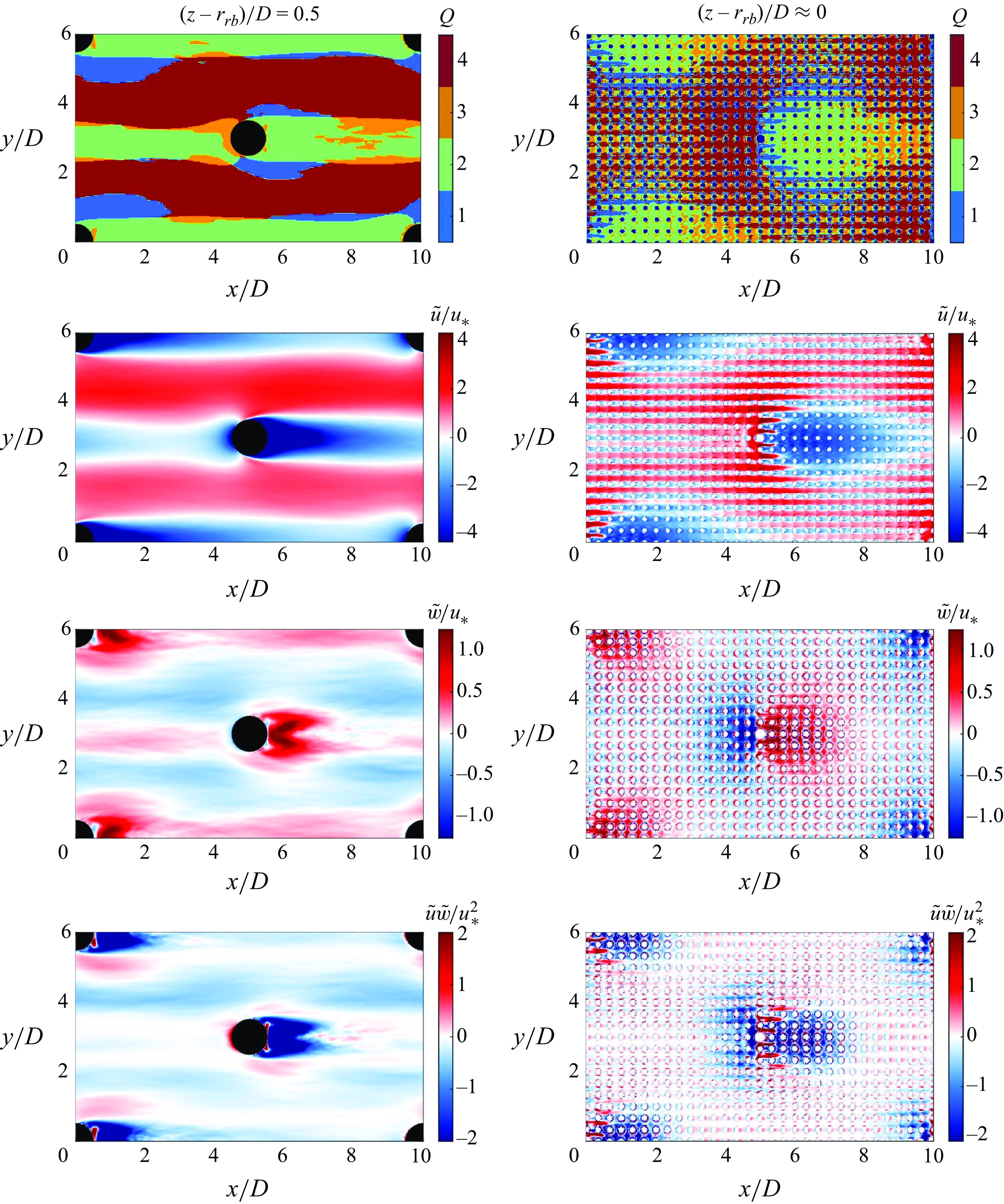
The region downstream of the boulders at mid-depth is characterised by Q2-type events, with negative spatial fluctuations of streamwise velocity $\tilde {u}$
, and positive vertical velocity fluctuations
$\tilde {u}$
, and positive vertical velocity fluctuations $\tilde {w}$
. In the high-velocity regions between the boulders, long Q4 regions are observed with small pockets of Q1 at the sides of the boulders, where the spatial fluctuations of vertical velocity become positive. These patterns persists as the horizontal plane moves closer to the rough bed, as shown in the right-hand panels of figure 15. At
$\tilde {w}$
. In the high-velocity regions between the boulders, long Q4 regions are observed with small pockets of Q1 at the sides of the boulders, where the spatial fluctuations of vertical velocity become positive. These patterns persists as the horizontal plane moves closer to the rough bed, as shown in the right-hand panels of figure 15. At $(z-r_{rb})/D \approx 0$
we still observe mostly Q2 events in the wakes of the boulders, Q4 events in the high streamwise velocity region between boulders and Q1 events on the edge of the wakes. However, significant changes are observed near the rough bed, since the variability of all the quantities is mostly observed between the roughness elements. Another important difference is the switch from Q2 to mostly Q4 (also some presence of Q3 and Q1) in the region upstream of the boulders when moving from the mid-boulder elevation to the top of the rough bed. The highest local form-induced stresses as illustrated in figure 15 (bottom row) are found in the wake of the boulders and are mostly negative stresses.
$(z-r_{rb})/D \approx 0$
we still observe mostly Q2 events in the wakes of the boulders, Q4 events in the high streamwise velocity region between boulders and Q1 events on the edge of the wakes. However, significant changes are observed near the rough bed, since the variability of all the quantities is mostly observed between the roughness elements. Another important difference is the switch from Q2 to mostly Q4 (also some presence of Q3 and Q1) in the region upstream of the boulders when moving from the mid-boulder elevation to the top of the rough bed. The highest local form-induced stresses as illustrated in figure 15 (bottom row) are found in the wake of the boulders and are mostly negative stresses.
Figure 16 also presents the cross-sectional distribution of longitudinal-averaged $\tilde {u}\tilde {w}$
together with transverse-averaged
$\tilde {u}\tilde {w}$
together with transverse-averaged $\tilde {u}\tilde {w}$
in the vertical plane. Patterns of
$\tilde {u}\tilde {w}$
in the vertical plane. Patterns of $\tilde {u}\tilde {w}$
observed in figure 16 result from the combined contribution of wake turbulence and SCs to streamwise (
$\tilde {u}\tilde {w}$
observed in figure 16 result from the combined contribution of wake turbulence and SCs to streamwise ( $\tilde {u}$
) and vertical (
$\tilde {u}$
) and vertical ( $\tilde {w}$
) velocity disturbances. Namely, the upward flow (positive
$\tilde {w}$
) velocity disturbances. Namely, the upward flow (positive $\tilde {w}$
coming from SC cells, see figure 4) together with the slow streamwise velocity at the boulders locations (negative
$\tilde {w}$
coming from SC cells, see figure 4) together with the slow streamwise velocity at the boulders locations (negative $\tilde {u}$
coming from the wakes) produce large and negative
$\tilde {u}$
coming from the wakes) produce large and negative $\tilde {u}\tilde {w}$
. Similarly, the downward flow between the boulders in the transverse direction and the high streamwise velocities in this regions also generate high negative
$\tilde {u}\tilde {w}$
. Similarly, the downward flow between the boulders in the transverse direction and the high streamwise velocities in this regions also generate high negative $\tilde {u}\tilde {w}$
.
$\tilde {u}\tilde {w}$
.
(a) Cross-sectional distribution of longitudinal-averaged $\tilde {u}\tilde {w}$
and (b) vertical plane of transverse-averaged
$\tilde {u}\tilde {w}$
and (b) vertical plane of transverse-averaged $\tilde {u}\tilde {w}$
.
$\tilde {u}\tilde {w}$
.
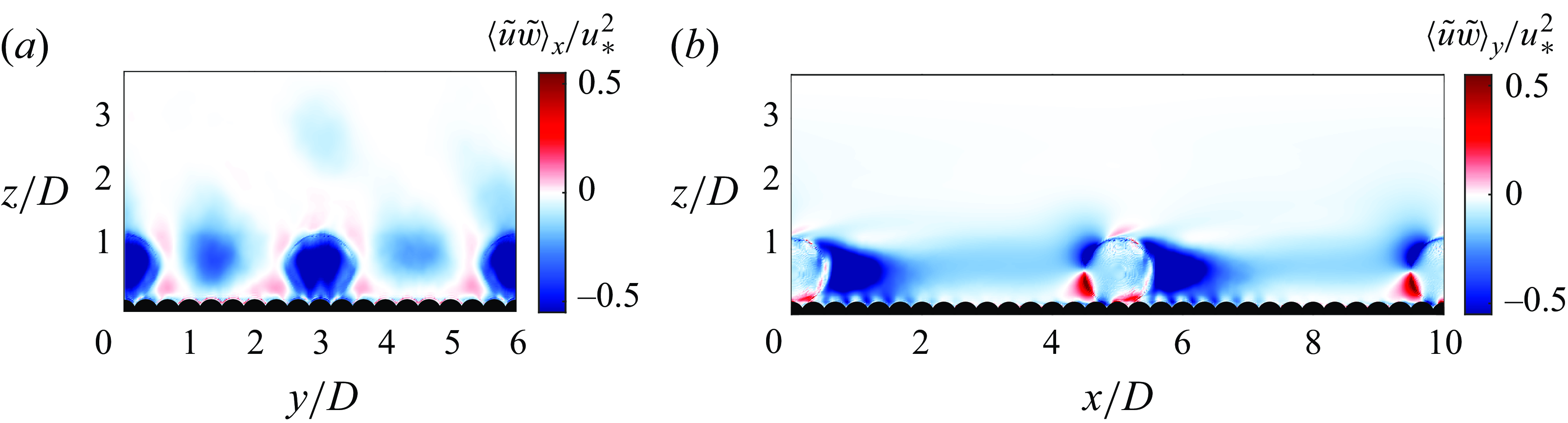
As it was shown with the quadrant maps, form-induced stresses are generated due to the combined effect of SCs and roughness-induced turbulence. In this regard, Nikora et al. (Reference Nikora, Stoesser, Cameron, Stewart, Papadopoulos, Ouro, McSherry, Zampiron, Marusic and Falconer2019) proposed partitioning the total form-induced stress into these two contributions based on the idea that they usually act on two separate scales. However, in the case of the present study, SC cells have a size which is of the same order of magnitude as the turbulent wake length scale, and therefore, it is not possible to separate roughness-scale effects from SC effects in the region within the boulders.
The quadrant map reveals distinct spatial regions corresponding to the different quadrants, with well-defined boundaries. The clear delineation of these regions stems from the strong spatial coherence of the time-averaged flow, which is driven by the 3-D wake turbulence generated by the boulder array and the induced SCs. While the quadrant maps proposed by Pokrajac et al. (Reference Pokrajac, Campbell, Nikora, Manes and McEwan2007) provide spatial distributions for each quadrant, they do not give information on the magnitude, direction or coherence of the velocity fluctuations within these regions. To address this limitation, we also analyse quadrant diagrams based on the spatial velocity fluctuations $\tilde {u}$
and
$\tilde {u}$
and $\tilde {w}$
. This approach enables detection of persistent spatial patterns in the time-averaged flow, which is particularly useful for studying wakes. For example, if the time-averaged flow is random in space, the quadrant diagram points (
$\tilde {w}$
. This approach enables detection of persistent spatial patterns in the time-averaged flow, which is particularly useful for studying wakes. For example, if the time-averaged flow is random in space, the quadrant diagram points ( $\tilde {u}$
,
$\tilde {u}$
, $\tilde {w}$
) will be scattered. Conversely, a distinct pattern in their distribution indicates a spatially organised time-averaged flow. As noted by Pokrajac et al. (Reference Pokrajac, Campbell, Nikora, Manes and McEwan2007), the radius of the vector in the quadrant diagram measured from the origin represents the magnitude of the form-induced velocity, while the angle indicates the direction of the flow.
$\tilde {w}$
) will be scattered. Conversely, a distinct pattern in their distribution indicates a spatially organised time-averaged flow. As noted by Pokrajac et al. (Reference Pokrajac, Campbell, Nikora, Manes and McEwan2007), the radius of the vector in the quadrant diagram measured from the origin represents the magnitude of the form-induced velocity, while the angle indicates the direction of the flow.
Figure 17 shows the quadrant diagram at different elevations with points that are coloured based on their position in the horizontal plane. The quadrant at the top of the rough bed depicts a scattered cloud of points, indicating that the roughness elements at the bed do not induce a spatially persistent organisation of the time-averaged flow. From just above the rough bed to the top of the boulders, a well-defined spatial profile of the time-averaged flow emerges. Points marked in black, which represent the wake of the boulders, exhibit larger streamwise velocity fluctuations compared with vertical components, creating an elongated structure. This structure extends from slightly above the rough bed to just past the mid-boulder level, where it diminishes significantly. The largest disturbances (points with the greatest radius in the quadrant diagram) are observed directly behind the boulders and decrease downstream.
Quadrant diagrams for different elevations, including from the top of the rough bed to slightly above the boulders. Points are coloured according to their location in the horizontal plane as depicted in the schematic figure at the top.
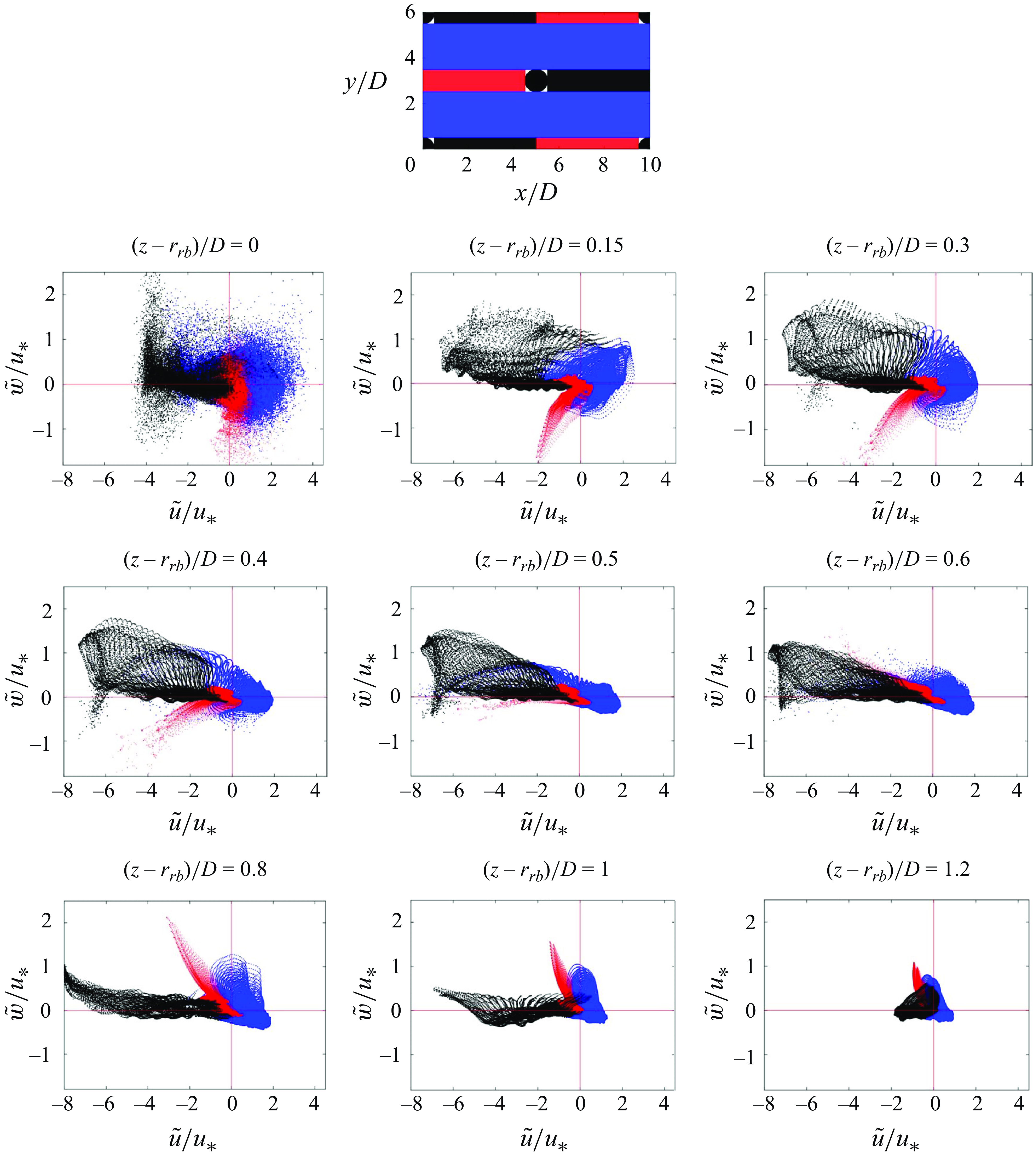
An important implication of this pattern is that the spatial structure associated with the wake of the boulders, shown in black, contributes significantly to the form-induced stress up to the mid-boulder level. This structure also represents a large portion of the contribution from Q2, as it is characterised by high values of both streamwise and vertical velocity fluctuations. At mid-boulder elevation, where the form-induced stress profile peaks globally, the stress reaches $\langle \tilde {u}\tilde {w}\rangle /u_*^2 = -0.16$
, which is close to the total contribution (
$\langle \tilde {u}\tilde {w}\rangle /u_*^2 = -0.16$
, which is close to the total contribution ( $73\,\%$
) from Q2 at this level (
$73\,\%$
) from Q2 at this level ( $\langle \tilde {u}\tilde {w}\rangle /u_*^2 = -0.22$
), and a substantial portion of the total stress (
$\langle \tilde {u}\tilde {w}\rangle /u_*^2 = -0.22$
), and a substantial portion of the total stress ( $\langle \tilde {u}\tilde {w}\rangle /u_*^2 = -0.3$
). This pattern does not appear at the top of the rough bed, where positive stresses (corresponding to Q3) induced by the roughness elements are also present in the wake of the boulders. The rough bed consists of hemispheres arranged in a skimming regime, interfering strongly with each other, whereas the boulders belong to an isolated regime with the wakes developing freely.
$\langle \tilde {u}\tilde {w}\rangle /u_*^2 = -0.3$
). This pattern does not appear at the top of the rough bed, where positive stresses (corresponding to Q3) induced by the roughness elements are also present in the wake of the boulders. The rough bed consists of hemispheres arranged in a skimming regime, interfering strongly with each other, whereas the boulders belong to an isolated regime with the wakes developing freely.
6. Double-averaged kinetic energy conservation equation
6.1. Double-averaged normal stresses and kinetic energy
To assess the contribution of form-induced stresses to DKE and compare it with the contribution of turbulent stresses to TKE, figure 18 presents the profiles of normal turbulent and form-induced stresses, as well as the evolution of TKE and DKE with height. The normal streamwise form-induced stress is larger than the turbulent counterpart across most of the region between the bed and the top of the boulders, highlighting the significant role of wake turbulence in generating additional stresses. While all turbulent-stress components contribute to TKE, only the streamwise component of form-induced stresses is considerable, being much larger than the spanwise and vertical stresses coming from SCs. These larger values of $\langle \tilde {u}\tilde {u} \rangle$
compared with
$\langle \tilde {u}\tilde {u} \rangle$
compared with $\langle \tilde {v}\tilde {v} \rangle$
and
$\langle \tilde {v}\tilde {v} \rangle$
and $\langle \tilde {w}\tilde {w} \rangle$
have been consistently observed in previous studies, regardless of bed shape and configuration (Yuan & Piomelli Reference Yuan and Piomelli2014; Fang et al. Reference Fang, Han, He and Dey2018). Conversely, no clear tendencies exist for the two other components but depend on the rough-surface topography. The large values of streamwise form-induced stress arise from the strong spatial variations generated by the boulder array (see the
$\langle \tilde {w}\tilde {w} \rangle$
have been consistently observed in previous studies, regardless of bed shape and configuration (Yuan & Piomelli Reference Yuan and Piomelli2014; Fang et al. Reference Fang, Han, He and Dey2018). Conversely, no clear tendencies exist for the two other components but depend on the rough-surface topography. The large values of streamwise form-induced stress arise from the strong spatial variations generated by the boulder array (see the $\tilde {u}$
map in figure 15). Even though the streamwise form-induced stresses are significantly larger than their turbulent counterparts, DKE remains smaller than TKE throughout nearly the entire water column. This is because turbulent stresses in the spanwise and vertical directions are large, while the corresponding form-induced stresses are negligible. Local peaks of TKE, DKE and normal streamwise stress are observed near the top of the rough bed. Additionally, similar to the shear-stress profile, global peaks for both form-induced and turbulent stresses are found at the middle and top of the boulders height, respectively, specially streamwise normal stresses and kinetic energy (see figure 5
b for comparison with local TKE values).
$\tilde {u}$
map in figure 15). Even though the streamwise form-induced stresses are significantly larger than their turbulent counterparts, DKE remains smaller than TKE throughout nearly the entire water column. This is because turbulent stresses in the spanwise and vertical directions are large, while the corresponding form-induced stresses are negligible. Local peaks of TKE, DKE and normal streamwise stress are observed near the top of the rough bed. Additionally, similar to the shear-stress profile, global peaks for both form-induced and turbulent stresses are found at the middle and top of the boulders height, respectively, specially streamwise normal stresses and kinetic energy (see figure 5
b for comparison with local TKE values).
(a) Normal turbulent (triangles) and form-induced stresses (circles). The three components that are shown correspond to the streamwise (black), spanwise (blue) and vertical (red). (b) The TKE (triangles) and DKE (circles) profiles.
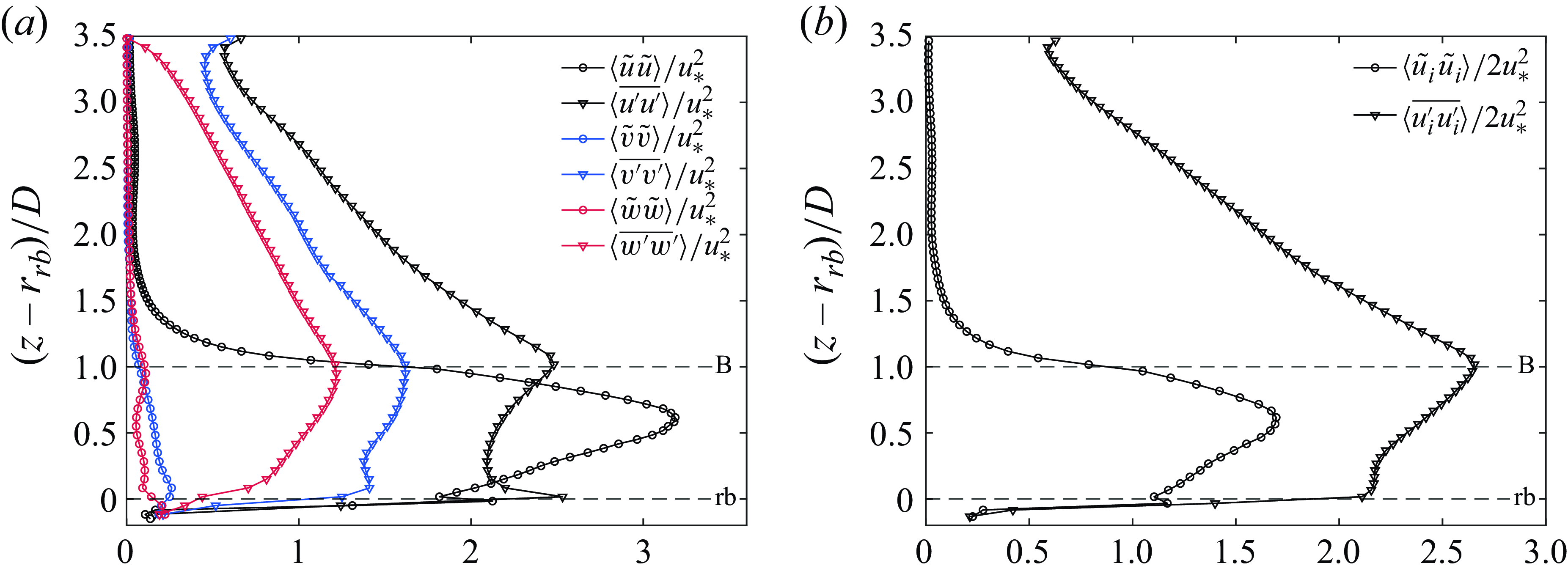
6.2. The MKE, TKE and DKE budgets
The analysis of the 3-D flow generated around the roughness elements from the perspective of the double-averaged energy budgets given by (4.3)–(4.5) can provide insights into the mechanisms of production, transport and dissipation of MKE, TKE and DKE with the water depth. In figure 19 we show vertical profiles of the different terms of the energy budgets. Positive values are a gain while negative ones indicate an energy loss. Drag terms ( $I_p + I_v$
) and turbulent dissipation (
$I_p + I_v$
) and turbulent dissipation ( $\epsilon _{TT}$
) are estimated as a residual of (4.3) and (4.5), respectively. In the MKE budget, energy is injected by gravity through the entire water column (
$\epsilon _{TT}$
) are estimated as a residual of (4.3) and (4.5), respectively. In the MKE budget, energy is injected by gravity through the entire water column ( $S_g$
in MKE). Then, energy is distributed by the transport terms from the excess energy region above the roughness elements to the deficit energy zone between them. Almost no MKE is dissipated since terms
$S_g$
in MKE). Then, energy is distributed by the transport terms from the excess energy region above the roughness elements to the deficit energy zone between them. Almost no MKE is dissipated since terms $\epsilon _{MM}$
and
$\epsilon _{MM}$
and $\epsilon _{DM}$
in (4.3) are close to zero. Near the rough bed, MKE is mainly transported by turbulent stresses (
$\epsilon _{DM}$
in (4.3) are close to zero. Near the rough bed, MKE is mainly transported by turbulent stresses ( $TM_T$
) toward a layer of 0.1D below and above the bed roughness surface. A smaller fraction of MKE is also transported by form-induced stresses (
$TM_T$
) toward a layer of 0.1D below and above the bed roughness surface. A smaller fraction of MKE is also transported by form-induced stresses ( $TM_D$
) inside the rough bed. Within the boulder region, MKE is transported toward the first half of the layer (closer to the rough bed) from the second half (closer to the boulder top) by form-induced stresses (
$TM_D$
) inside the rough bed. Within the boulder region, MKE is transported toward the first half of the layer (closer to the rough bed) from the second half (closer to the boulder top) by form-induced stresses ( $TM_D$
). Conversely, turbulent stresses (
$TM_D$
). Conversely, turbulent stresses ( $TM_T$
) transport the excess of MKE in the opposite direction, from slightly above the rough bed to the boulders top.
$TM_T$
) transport the excess of MKE in the opposite direction, from slightly above the rough bed to the boulders top.
Energy budgets of MKE, DKE and TKE from top to bottom, normalised by $h/u_*^3$
. Viscous transport and dissipation terms are negligible and not shown in the plot. We show the region of the water depth between the rough bed and above the boulders.
$h/u_*^3$
. Viscous transport and dissipation terms are negligible and not shown in the plot. We show the region of the water depth between the rough bed and above the boulders.
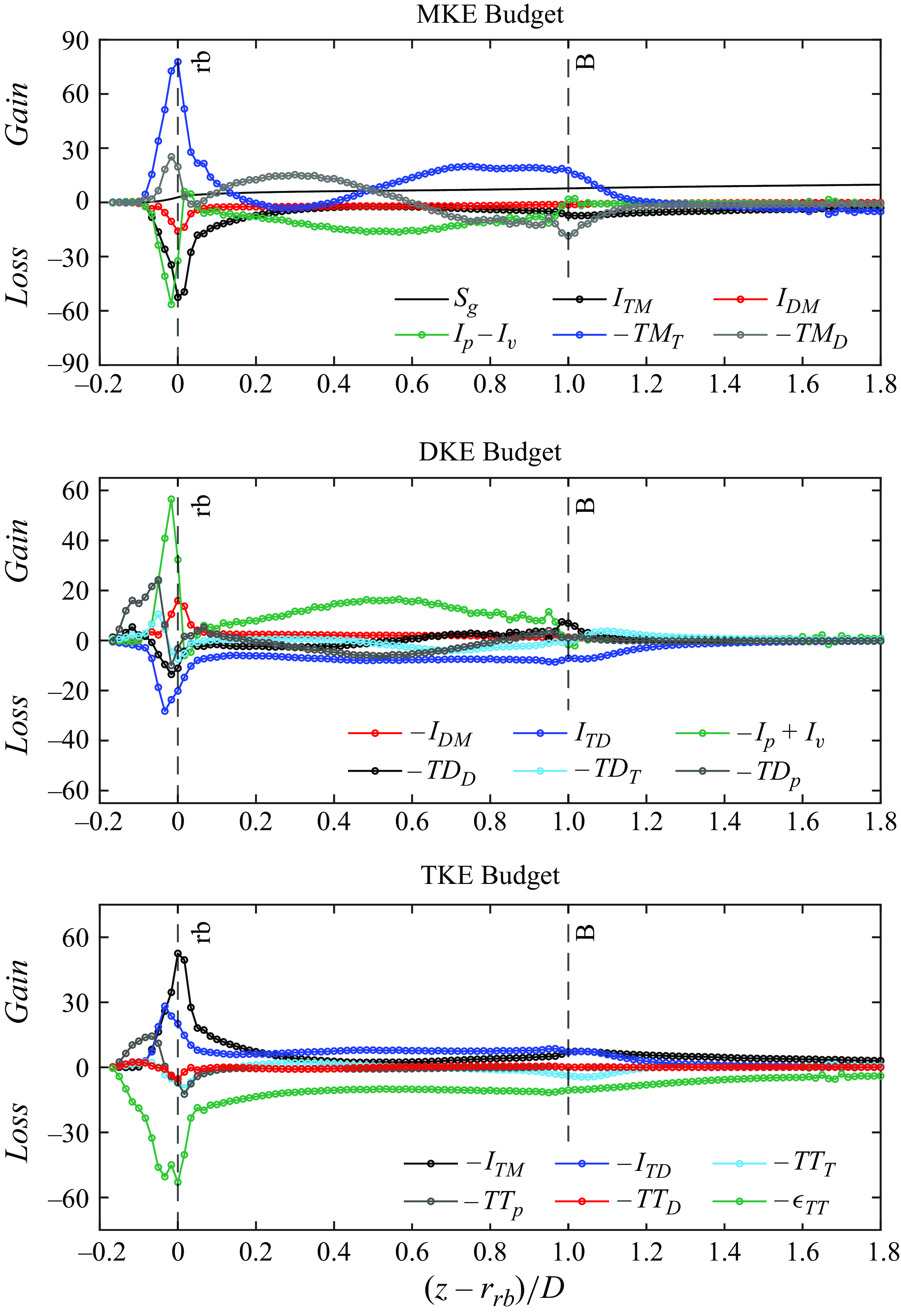
From the energy flux to the rough bed, a significant fraction is transferred to the turbulent field by the term $I_{TM}$
, and there is a large contribution to pressure (
$I_{TM}$
, and there is a large contribution to pressure ( $I_p$
) and viscous drag (
$I_p$
) and viscous drag ( $I_v$
), while a smaller fraction is transferred to the form-induced field by the term
$I_v$
), while a smaller fraction is transferred to the form-induced field by the term $I_{DM}$
. Both the drag (
$I_{DM}$
. Both the drag ( $I_p$
and
$I_p$
and $I_v$
) and
$I_v$
) and $I_{DM}$
correspond to energy that is transformed from MKE into DKE. On the other hand, from the energy transported towards the boulder layer, the largest fraction is used to generate pressure (
$I_{DM}$
correspond to energy that is transformed from MKE into DKE. On the other hand, from the energy transported towards the boulder layer, the largest fraction is used to generate pressure ( $I_p$
) and viscous drag (
$I_p$
) and viscous drag ( $I_v$
) thus producing DKE, while a smaller fraction is also transferred directly to the turbulent (
$I_v$
) thus producing DKE, while a smaller fraction is also transferred directly to the turbulent ( $I_{TM}$
) and form-induced fields (
$I_{TM}$
) and form-induced fields ( $I_{DM}$
). The DKE production that results from the action of form-induced stresses against the mean flow (
$I_{DM}$
). The DKE production that results from the action of form-induced stresses against the mean flow ( $I_{DM}$
in MKE) is smaller but comparable in magnitude to turbulent production (
$I_{DM}$
in MKE) is smaller but comparable in magnitude to turbulent production ( $I_{TM}$
). However, most of the energy transferred from the mean flow to the form-induced field comes from pressure and viscous drag, which show a larger magnitude between the rough bed and the array of boulders.
$I_{TM}$
). However, most of the energy transferred from the mean flow to the form-induced field comes from pressure and viscous drag, which show a larger magnitude between the rough bed and the array of boulders.
In the form-induced field, from the energy injected from the mean field, an important fraction of DKE is transformed to TKE through $I_{TD}$
. The excess of DKE (i.e. production minus dissipation) within the boulders is transported toward the rough bed by pressure (
$I_{TD}$
. The excess of DKE (i.e. production minus dissipation) within the boulders is transported toward the rough bed by pressure ( $TD_{p}$
) and turbulent stresses (
$TD_{p}$
) and turbulent stresses ( $TD_{T}$
) and from within the rough bed to the top of the boulders by form-induced stresses (
$TD_{T}$
) and from within the rough bed to the top of the boulders by form-induced stresses ( $TD_{D}$
). Almost no form-induced energy is dissipated since
$TD_{D}$
). Almost no form-induced energy is dissipated since $\epsilon _{DD}$
and
$\epsilon _{DD}$
and $\epsilon _{MD}$
are close to zero (and therefore not plotted in figure 19). In the region within and slightly above the rough bed, the terms of (4.3) do not balance since the conditions for which the DKE budget was derived are not fulfilled in that layer. On the other hand, in the turbulent field, energy is injected from the mean flow by
$\epsilon _{MD}$
are close to zero (and therefore not plotted in figure 19). In the region within and slightly above the rough bed, the terms of (4.3) do not balance since the conditions for which the DKE budget was derived are not fulfilled in that layer. On the other hand, in the turbulent field, energy is injected from the mean flow by $I_{TM}$
and from the form-induced field by
$I_{TM}$
and from the form-induced field by $I_{TD}$
where the latter is smaller than but comparable to the former around the rough bed, and even larger around the boulders. Slightly above the boulders (from
$I_{TD}$
where the latter is smaller than but comparable to the former around the rough bed, and even larger around the boulders. Slightly above the boulders (from $(z-r_{rb})/D=1.3$
), the TKE production terms are significantly larger than the transport terms, indicating a balance between production and dissipation as observed by Yuan & Piomelli (Reference Yuan and Piomelli2014) and Zampiron et al. (Reference Zampiron, Cameron and Nikora2021). Within the roughness elements, even when production terms are larger than transport terms, the latter do not vanish, and therefore production and dissipation of energy are not at equilibrium. Moreover, since almost no dissipation occurs in the mean and form-induced fields, all the potential energy injected by gravity is finally dissipated by the turbulent field.
$(z-r_{rb})/D=1.3$
), the TKE production terms are significantly larger than the transport terms, indicating a balance between production and dissipation as observed by Yuan & Piomelli (Reference Yuan and Piomelli2014) and Zampiron et al. (Reference Zampiron, Cameron and Nikora2021). Within the roughness elements, even when production terms are larger than transport terms, the latter do not vanish, and therefore production and dissipation of energy are not at equilibrium. Moreover, since almost no dissipation occurs in the mean and form-induced fields, all the potential energy injected by gravity is finally dissipated by the turbulent field.
7. Conclusions
In this investigation we study the flow over a rough bed with an array of boulders using LES, based on the experiments of Papanicolaou et al. (Reference Papanicolaou, Kramer, Tsakiris, Stoesser, Bomminayuni and Chen2012). The complex 3-D flow dynamics, driven by strong interactions between bed roughness and boulder wakes, significantly influences larger-scale processes when analysed using averaged velocity profiles that are commonly employed in global analyses.
We show that a roughness parameterisation with the novel approach by Meneveau et al. (Reference Meneveau, Hutchins and Chung2024) captures near-bed conditions well, but wake effects from large boulders strongly impact velocity and turbulence statistics across a significant portion of the water column. The double-averaged velocity profile obtained here is not universal, but strongly depends on the roughness shape and bed configuration in the region $(z-r_{rb})/D \approx 0-2.5$
. The results also show that the profile may be approximated by a third-order polynomial, resulting from the strong velocity gradient at the rough bed surface. In the boulder region, a linear velocity profile is obtained from
$(z-r_{rb})/D \approx 0-2.5$
. The results also show that the profile may be approximated by a third-order polynomial, resulting from the strong velocity gradient at the rough bed surface. In the boulder region, a linear velocity profile is obtained from $(z-r_{rb})/D \approx 0.3-1.75$
, indicating a constant averaged velocity gradient. The method formulated by Meneveau et al. (Reference Meneveau, Hutchins and Chung2024) gives a good estimation of
$(z-r_{rb})/D \approx 0.3-1.75$
, indicating a constant averaged velocity gradient. The method formulated by Meneveau et al. (Reference Meneveau, Hutchins and Chung2024) gives a good estimation of $k_s$
from the geometry of the bed and assuming a logarithmic profile, but additional work is needed to elucidate the critical parameters that characterise the velocity profile in the roughness layer.
$k_s$
from the geometry of the bed and assuming a logarithmic profile, but additional work is needed to elucidate the critical parameters that characterise the velocity profile in the roughness layer.
To gain insight into the influence of turbulent coherent structures, a double-averaged decomposition of the flow field is applied, connecting the dynamics of these coherent structures to the spatial distribution of stresses and the energy balance along the vertical direction. This study provides the first detailed statistical analysis of velocity, energy and momentum in rough beds with low relative submergence, and the upscaling of turbulent statistics. We focus on evaluating the averaged flow velocity and stresses to unpack the effects of the 3-D nature of the wake turbulence generated by the rough bed and the array of boulders within the momentum and energy budgets.
The results show that the shear layer generated at the boulders crest, as well as the local turbulence produced by the rough bed, result in large values of TKE and Reynolds shear stress, including significant spatial variations of these quantities, which are key factors influencing sediment transport. The instantaneous flow is characterised by large vorticity and coherent structures in the wake of the boulders emerging from the shear layer and advected downstream. Based on the streamwise momentum equation, we evaluate the different contributions to shear stress, focusing on the effective shear stress from turbulent and form-induced components, excluding the drag from roughness elements. This effective stress, which has important implications for bedload transport, accounts for half of the total at the rough bed surface, highlighting the strong drag induced by the boulders. Form-induced stresses are larger around the boulder array due to low relative submergence and the isolated regime. Their peak nearly matches turbulent stress at mid-boulder elevation, reaching $37\,\%$
of the total shear stress.
$37\,\%$
of the total shear stress.
We apply the quadrant analysis of Pokrajac et al. (Reference Pokrajac, Campbell, Nikora, Manes and McEwan2007) to assess the contributions to form-induced stresses based on the sign of time-averaged spatial velocity fluctuations. Negative events (Q2, Q4) dominate over positive ones (Q1, Q3) throughout the water column, generating additional fluid stresses beyond drag effects. The Q2 events concentrate in boulder wakes, Q4 in high-velocity regions between boulders and Q1 at the wake edges, reflecting the strong spatial coherence of the 3-D wake turbulence. The high magnitude negative form-induced stresses observed result from the combined influence of roughness-induced turbulence and SCs, where the elongated wake structure carries a significant fraction of form-induced stresses counteracting energy dissipation by drag.
The results show that the boulders and the rough bed generate significant form-induced kinetic energy in the entire water column, which is comparable to the TKE in the layers surrounding the roughness elements. Large DKE is explained entirely by the contribution of normal streamwise form-induced stresses, as opposed to TKE, where all components are significant. The energy budget reveals that most of DKE production comes from drag (from the mean flow) and a smaller fraction from the work done by the mean flow against form-induced stresses. The present results illustrate how this significant form-induced kinetic energy generated due to drag is then transferred to the turbulent field to finally be dissipated.
These findings highlight the role of roughness elements in generating form-induced stresses, which must be considered when assessing potential sediment transport without including the drag component. Our results emphasise the influence of wake turbulence in producing form-induced stresses that partly compensate the energy loss due to drag. Energy budgets show how drag energy transfers from DKE to TKE before dissipating. Future work will incorporate mobile sediments to link transport across scales (Escauriaza et al. Reference Escauriaza, González, Williams and Brevis2023), relating global bedload fluxes to effective shear stress, and local transport and fluctuations in sediment velocities and concentration to spatial variations of the flow field.
Acknowledgements
We thank the second reviewer for the insightful comments that were gratefully incorporated.
Funding
This work has been supported by ONR-Global grant N62909-23-1-2004 and the computational resources provided by supercomputing infrastructure of the NLHPC (ECM-02). The graduate studies of M.B. were funded by CONICYT-PFCHA/Doctorado Nacional/2020-21200308.
Declaration of interests
The authors report no conflict of interest.


 Open access