

Introduction
The relative importance of mass and volume change to sea-level rise is of great practical as well as pure scientific interest since their relative response to climate forcing may be very different. We may expect that a change in volume associated with rising temperatures will be relatively smooth, while potential ice-sheet instabilities may produce very rapid and large changes in sea level. The relative mass and volume change is also of interest because it takes ~50 times more energy to raise sea level by ocean heating than by ice melting (Reference TrenberthTrenberth, 2009).
There are two main methods of estimating sea-level rise. (1) The contribution from each component of the system can be estimated: glaciers and small ice caps (GSIC), the Greenland ice sheet (GIS), the Antarctic ice sheet, thermal expansion (TS), and changes in terrestrial storage (T). (2) The total observed by tide gauges, complemented since 1993 with satellite altimeter measurements, can be estimated. If these two estimates agree, then we call the sea-level budget closed. Some authors claim that the sea-level budget is closed (Reference DominguesDomingues and others, 2008), despite, or perhaps utilizing, the large errors involved in the contributors, but others claim that the best estimates of the relative contributions leave a significant discrepancy with observed sea level (Reference Jevrejeva, Moore and GrinstedJevrejeva and others, 2008b).
In this paper, we provide estimates of the various contributions and discuss how close the sum of the parts is to the observed total sea-level rise. We show that the best estimates of the sea-level components result in a satisfactory agreement with observed sea level since 1955 only if we include estimates for polar small glaciers (PSG) from indirect modeling, which seem to have been subject to mu‘ch more negative mass balance than more temperate glaciers. We also discuss the much less well-studied, uncertain earlier sea-level component records from 1850 to 1950. Despite the uncertainties, some plausible features of the record may be extracted.
Data
We utilize 1023 time series of monthly mean relative sea level (RSL) from the Permanent Service for Mean Sea Level (PSMSL) database (Reference Woodworth and PlayerWoodworth and Player, 2003). RSL datasets were corrected for local datum changes and glacial isostatic adjustment (GIA) of the solid Earth (ICE 4G, VM2; Reference Peltier, Douglas, Kearney and LeathermanPeltier, 2001). We use a global sea-level (GSL) curve based on the ‘virtual station’ method (Reference Jevrejeva, Grinsted, Moore and HolgateJevrejeva and others, 2006) which overcomes geographical bias by accounting for the spacing between stations in creating sea-level curves for each of 13 ocean basins. Since about 1950, coverage by tide gauges has been very thorough, but especially in the 18th and 19th centuries there were very few tide gauges, and all were located in Europe, so the issue of how representative a particular tide gauge station in only one basin is of GSL variations was estimated using bootstrap methods (Reference Grinsted, Moore and JevrejevaGrinsted and others, 2009). Our GSL trend estimate of 2.4±1.0mma–1 for the period 1993–2000 is comparable with the 2.6±0.7mma–1 sea-level rise calculated from TOPEX/Poseidon altimeter measurements (Reference Grinsted, Moore and JevrejevaGrinsted and others, 2009). The GSL curve also produces good estimates of the volcanic impacts on sea level (Reference Grinsted, Moore and JevrejevaGrinsted and others, 2007), and has been used to reconstruct sea level over the past 2000 years (Reference Grinsted, Moore and JevrejevaGrinsted and others, 2009; Reference Jevrejeva, Grinsted and MooreJevrejeva and others, 2009). The GSL reconstruction (together with calculated errors) is available from http://www.psmsl.org/products/reconstructions/jevrejevaetal2006.php
Steric sea level is based on estimates of Global Ocean Heat Content (GOHC) data and is discussed by Reference Levitus, Antonov, Boyer, Locarnini, Garcia and MishonovLevitus and others (2009) for the period 1955–2008. This time period was affected by systematic errors in the heat measurements from the Argo profiling float data that were included in earlier heat-content estimates (e.g. Reference Levitus, Antonov and BoyerLevitus and others, 2005). We use several estimates of steric sea level derived from the ocean heat-content data, but mainly rely on the values from Reference DominguesDomingues and others (2008), where we have added 20% to the 0–700m steric sea-level values, as those authors suggest, to account for the deeper ocean contribution. We return to this contentious issue later. We also make use of an estimate of steric sea level from a climate model (Reference Gregory, Lowe and TettGregory and others, 2006) to extend the record back in time to 1850.
Data on past variations in GSIC come from Reference CogleyCogley (2009). We also estimate GSIC from the independent data on glacier termini positions from Reference Oerlemans, Dyurgerov and van de WalOerlemans and others (2007). This compensates for the very sparse data on glacier mass-balance estimates available prior to 1950 from Reference CogleyCogley (2009): prior to the 1910s, all measurements come from Swiss glaciers, only supplemented between the 1910s and the 1930s from Scandinavian glaciers. The GSIC have been consolidated into 5 year global averages of mass balance of glaciers from outside Greenland and Antarctica based on both direct glaciological surveys and geodetic surveys that together are quite reliable back to about 1955. A crucial point is how the dataset is extended to include the virtually unsampled smaller polar glaciers. Reference Kaser, Cogley, Dyurgerov, Meier and OhmuraKaser and others (2006) give three possible estimates based on correlations with either the whole dataset of measured glaciers or glaciers in Canada. In contrast, Reference Hock, deWoul, Radiá and DyurgerovHock and others (2009) use mass-balance modeling based on available meteorological station data to estimate the regional mass balance of under-sampled PSG. They computed a rate of 0.28 ±0.17 mma–1 for the period 1961–2004, and we use this rate for the 1955–2005 period.
Data on Greenland mass-balance (GIS) history come from Reference Rignot, Box, Burgess and HannaRignot and others (2008a). The GIS was sporadically surveyed typically by leveling across coast-to-coast transects in the early 20th century, but more complete direct observations were carried out in 1958. Reference CogleyCogley (2009) computed the mass balance in 5 year blocks for GSIC, and to make the data more comparable between the different sources we do the same for TS and GIS (assuming for GIS that the 1955–60 balance is the same as the 1958 measurement). This has the impact of removing much seasonal variability, hemispheric differences and noise due to annual snow accumulation variations. Post-1955 5 year 95% confidence intervals are <20% of the mass-balance estimates in GSIC (Reference CogleyCogley, 2009). The mass-balance estimates are summed to produce a relative sea-level curve over time in the figures we show to allow comparison with the GSL curve from tide gauges. We compute the error in GSL as the yearly standard error/ ![]() since autocorrelation within N=5 yearly blocks can be neglected and the data assumed to be independent.
since autocorrelation within N=5 yearly blocks can be neglected and the data assumed to be independent.
Results
In Figure 1 and Table 1 we show the major components of the 1955–2005 sea-level budget, and their sum compared with the GSL and its error. Since for most components accurate data exist only since about the mid-1950s, we use 1955 as the reference year. Also shown in Figure 1 is the estimation of TS from the climate model; the agreement of the curve with the Reference DominguesDomingues and others (2008) curve based on observations is reasonably close, at least in general shape and magnitude. Several things are clear from the plot:
Time series of anomalies in sea-level components from 1955 to 2005. GSL (black, with standard error as grey shaded region (Reference Jevrejeva, Grinsted, Moore and HolgateJevrejeva and others, 2006)); TS (red solid line, from Reference DominguesDomingues and others (2008) corrected for full ocean depth); modeled thermosteric (red dotted line (Reference Gregory, Lowe and TettGregory and others, 2006)). Cumulative mass balance as sea-level equivalents for: GSIC (blue; Reference CogleyCogley, 2009), GIS (green; Reference Rignot, Box, Burgess and HannaRignot and others, 2008a) and mountain glacier termini (cyan; Reference Oerlemans, Dyurgerov and van de WalOerlemans and others, 2007). Also shown are summed components (TS + GSIC + GIS + PSG; magenta). The 1955–60 period is the baseline for all datasets.
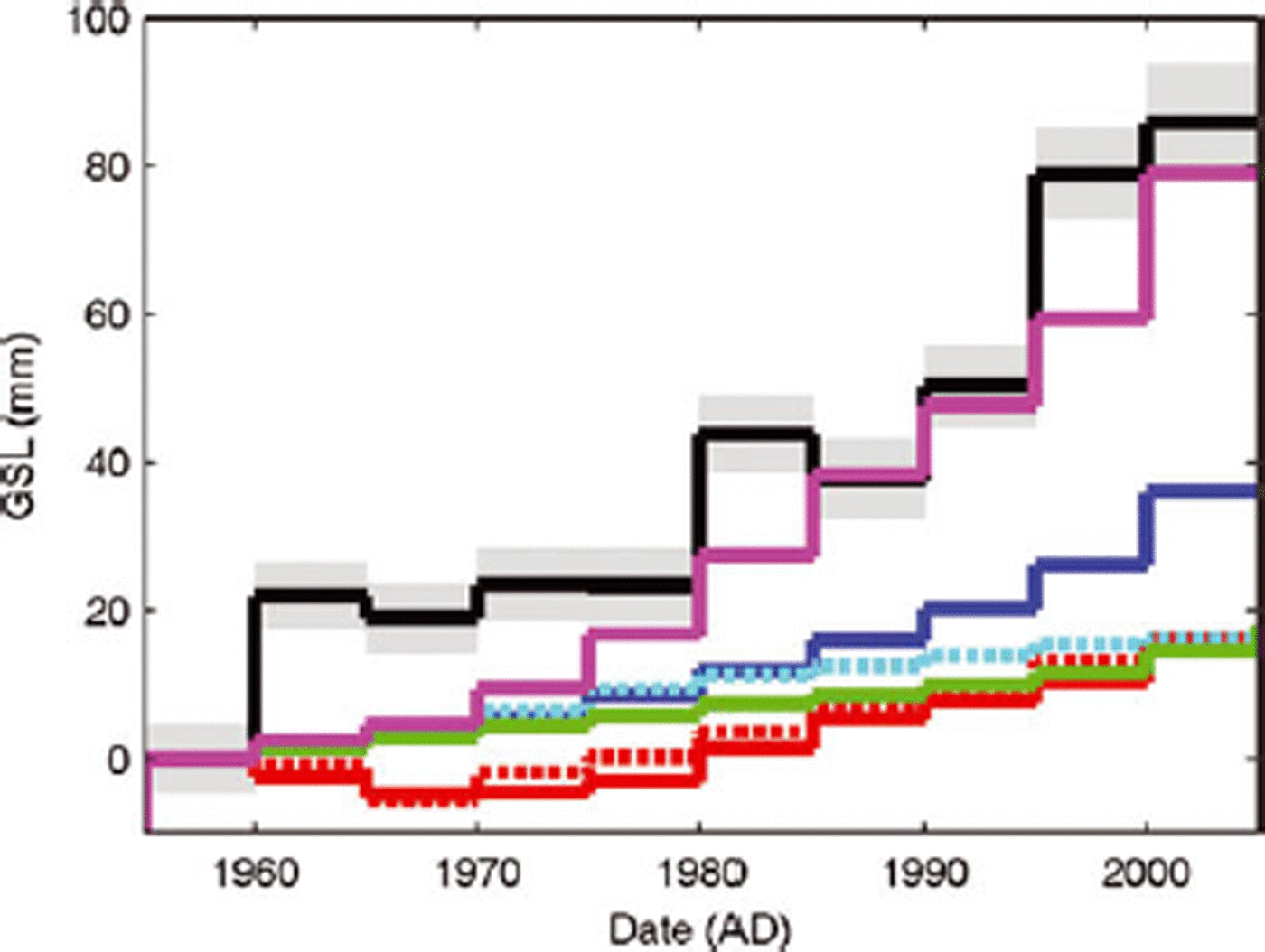
Contributions to the sea-level budget from 1955 to 2005
-
1. GSL is not particularly well correlated with TS (this has also been discussed by Jevrejeva and others, 2008). Despite corrections to the GOHC dataset (e.g. Reference Levitus, Antonov, Boyer, Locarnini, Garcia and MishonovLevitus and others, 2009), this remains the case.
-
2. Despite a considerable acceleration in mass loss from both the GIS and GSIC since 2000, the sea-level budget constructed using only GIS + GSIC + TS has a residual trend significant at the 93% level and amounting to 0.36mma–1, with a standard error of 0.18mma–1, accounting for 36% of the variance of the residual GSL. The sea-level budget can, however, be closed so that the residual trend is wholly insignificant by including the estimated contribution trend from polar small glaciers and ice caps (PSG) from Reference Hock, deWoul, Radiá and DyurgerovHock and others (2009).
-
3. The TS component is a much smaller component of GSL than GSIC. Indeed it is of similar magnitude to the mass loss from Greenland, or estimates of the contribution from polar mountain glaciers (Table 1).
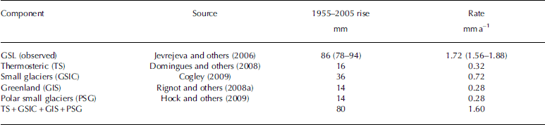
We investigate the longer-term sea-level budget in Figure 2 where we make use of an extended record of GSIC taken from both Reference Oerlemans, Dyurgerov and van de WalOerlemans and others (2007) and the approximately twice as large estimate from Reference CogleyCogley (2009), together with the modeled TS component from Reference Gregory, Lowe and TettGregory and others (2006). It is clear from this plot that:
Time series of anomalies in sea-level components from 1850 to 2005. Curves are as for Figure 1, with summed components (magenta dotted: modeled TS + GSIC + GIS). GIS is assumed to be zero prior to 1955, so the sum is just the blue and red dotted contribution from GSIC and modeled TS.
-
1. The TS component remained a small fraction of the sea-level budget back to the mid-19th century, where tide-gauge observations are sparse and errors in GSL become much larger than for the more recent part of the record.
-
2. The sea-level budget can be much better closed using the rates from Reference CogleyCogley (2009) than those from Reference Oerlemans, Dyurgerov and van de WalOerlemans and others (2007), and this would be true of whatever shape factor was used for the geometrical conversion of glacier termini position to glacier volume (Reference Oerlemans, Dyurgerov and van de WalOerlemans and others, 2007).
-
3. The rate of GSL rise between 1930 and 1950 was about as fast as in the post-2000 period, ~3mma–1. The sea-level curve is consistent with an accelerating trend of 0.01 mma–2 from about 1800; superimposed on the long-term acceleration are quasi-periodic fluctuations with a period of ~60 years (Reference Jevrejeva, Moore, Grinsted and WoodworthJevrejeva and others, 2008a). The only contributing information available is GSIC (though much less reliably than since 1955 (Reference CogleyCogley, 2009)). Figure 2 shows that GSIC were not likely to be the main factor in the rapid rise of GSL at that time. The rather slow changes in TS since 1955 suggest that rapid thermosteric response could only be responsible for the GSL changes if there were dramatic changes in ocean circulation. This implies that other sources of mass were most likely the cause of rising GSL: either from Greenland, as has been postulated during the warm 1920s and 1930s by Reference Rignot, Box, Burgess and HannaRignot and others (2008a), Antarctica or other smaller high-latitude glaciers.
Discussion
1955–2005 interval
We have shown that the sea-level budget may be reasonably closed using the PSG contribution estimated by Reference Hock, deWoul, Radiá and DyurgerovHock and others (2009). Support for this also comes from exploring the components of the budget with multiple linear regression. When we do this with TS, GSIC and GIS as forcing variables (and not including any trend for PSG), we find that TS (from Reference DominguesDomingues and others, 2008) has an unphysical, negative coefficient of –1.2±1.1, whereas we would expect a coefficient of 1. This is a marginally significant result. If we drop TS from the GSL forcing factors then the coefficient for GIS dominates (3.7±1.8) that from GSIC (1.1±1). This could be interpreted as suggesting that it is the GIS, or factors that correlate with it, that may be responsible for the missing sea-level component. Reference Hock, deWoul, Radiá and DyurgerovHock and others’ (2009) consideration of the polar glacier contribution suggested that most of the contribution was from the Antarctic Peninsula region (0.22±0.16mma–1), while the marginal Greenland and other High Arctic glaciers contributed much less. This finding would also be consistent with the inference of unaccounted melting from analyzing the Earth’s rotation (Reference Mitrovica, Wahr, Matsuyama, Paulson and TamisieaMitrovica and others, 2006), and with evidence of freshening of the oceans (Reference Ishii, Kimoto, Sakamoto and IwasakiIshii and others, 2006). Nevertheless the underlying driving force for the ice loss was the relatively greater warming trend in summer temperatures both in the Antarctic Peninsula and, since the 1990s, over Greenland (Reference Rignot, Box, Burgess and HannaRignot and others, 2008a; Reference Hock, deWoul, Radiá and DyurgerovHock and others 2009).
Observed sea level is complicated by many other forcing factors such as El Niño Southern Oscillation (ENSO), ocean dynamics and global water cycle, so the detailed observed response to individual eruptions contains very high noise. Reference Grinsted, Moore and JevrejevaGrinsted and others (2007) showed that the impact of volcanic activity on sea level was not simply a depression due to global cooling in the years after an eruption, but also a modification of the global water budget such that sea level rises significantly in the first year, followed later by a fall. Large volcanic eruptions inject aerosols into the stratosphere, and these aerosols reflect sunlight, causing global dimming and thus lower temperatures at the Earth surface. The cooling of the ocean surface causes less evaporation. As water flux from terrestrial reservoirs and river discharge continue, the combination of less evaporation and water flux results in a GSL rise of 6–12mm during the first year following the eruption. After ~1 year, stratospheric aerosols have been removed and evaporation reaches normal values. However, the river discharge is now reduced due to the low precipitation in the preceding year, so sea level drops by 4–10mm 2–3 years after the eruption. This interpretation is supported by observations of large reductions in both land precipitation and continental discharge following major volcanic eruptions (Reference Trenberth and DaiTrenberth and Dai, 2007), and modeled reductions in terrestrial storage caused by reductions in precipitation (Reference Milly, Cazenave and GenneroMilly and others, 2003).
The timing of volcanic eruptions is unaffected by the ENSO phase. Some eruptions will by chance occur in El Niño years. In contrast, it is plausible that an eruption would have some impact on the ENSO system; perhaps the cooling weakens the trade winds (a weakening being a precursor to El Niño events). We do not argue that volcanic eruptions trigger El Niño events; rather, we argue that it is important to not exclude the possibility of a volcanic influence on the ENSO system.
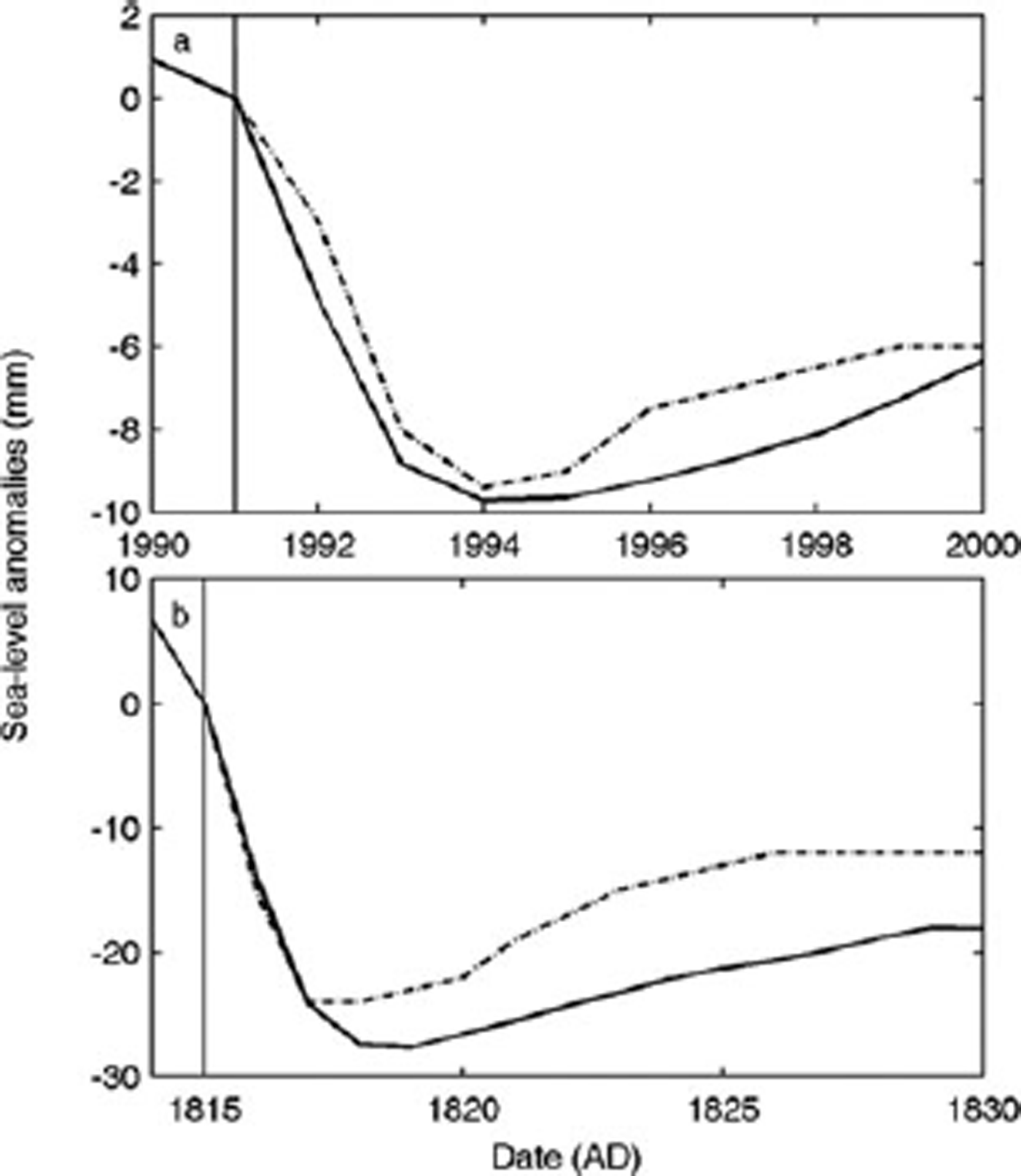
Interdecadal and multi-year variability in sea level has been attributed to ENSO and volcanic forcing. While the immediate atmospheric impacts of a large volcanic eruption tend to decay within a few years as stratospheric aerosol is removed (Reference RobockRobock, 2000), it has been realized that the impact on the oceans may be much more pervasive and could last a decade or more. Reference Stenchikov, Delworth, Ramaswamy, Stouffer, Wittenberg and ZengStenchikov and others (2009) use the CM2.1 climate system model to estimate the sea-level response of the large Tambora (Indonesia) 1815 and Pinatubo (Philippines) 1991 eruptions. The sea-level response is essentially determined in the Stenchikov model by the global ocean heat content change. To help interpret and attribute the causes of sea-level rise further, we use a semi-empirical model (Reference Jevrejeva, Moore and GrinstedJevrejeva and others, 2010) that realistically matches observed sea level over a range of timescales from multi-year to centennial scales. Figure 3 shows the Stenchikov modeled response compared with the model of sea level fitted to the GSL tide-gauge data. This means that for Tambora the model of Reference Jevrejeva, Moore and GrinstedJevrejeva and others (2010) must extrapolate well beyond the magnitude of volcanic eruptions observed over most of the tide-gauge measurement interval. Notice that both models predict about the same maximum response, the timing of the maximum drop, and have similar recovery curves. The Tambora response is about three times the Pinatubo response in both models. It is also clear that the volcanic response is primarily determined by heat content change rather than mass of ocean water on multi-year timescales. It also seems to be the case that our model produces a deeper drop than the Stenchikov model, perhaps because our model implicitly incorporates the full system response rather than simply ocean heat content.
Reference Stenchikov, Delworth, Ramaswamy, Stouffer, Wittenberg and ZengStenchikov and others (2009) (dashed curve) and our model (solid curve) sea-level anomaly responses to the Pinatubo 1991 eruption (a) and the Tambora 1815 eruption (b). Anomalies calculated relative to the sea level in the eruption year. Vertical line in both panels corresponds to the year of volcanic eruption.
The reduction in radiative forcing due to eruptions for the period 1880–2000 was estimated by Reference Jevrejeva, Grinsted and MooreJevrejeva and others (2009) to amount to a reduction of 7 cm in GSL relative to the level it would have reached had no eruptions occurred. The effect of the three large eruptions of the post-1955 period (Agung (Indonesia) 1963, El Chichón (Mexico) 1982 and Pinatubo 1991) was a depression in sea level for 5–10 years of ~5–10mm (Fig. 4) each.
Residual sea level (GSL – TS – GIS – GSIC – PSG; thick black line), TS (red line) and modeled sea-level response to volcanism (thin black curve). Also plotted is 12 month smoothed ENSO as calculated in the text (blue curve, right-hand scale).
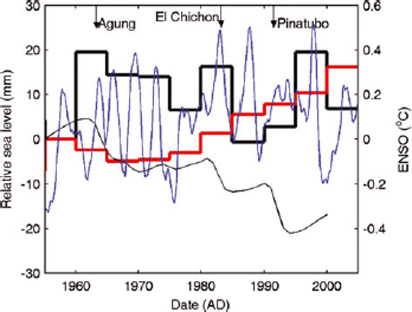
We use an estimate of ENSO activity (http://jisao.washington.edu/data/globalsstenso/globalsstenso18002010.ascii) calculated as the average sea surface temperature (SST) anomaly equatorward of 20˚ latitude (north and south) minus the average SST poleward of 20˚, which captures the low-frequency part of the ENSO phenomenon. Anomalies are with respect to the period 1950–79. The number of observations contributing is at least 1000 in each month and year beginning in the 1850s. The choice to calculate the index as the difference of two time series removes a spurious step-jump in SST observations at the onset of World War II that is associated with changes in measurement practices (Reference Folland and ParkerFolland and Parker, 1995). The difference also removes the common portion of the trend in SST.
In Figure 4 we examine the residual sea level together with the ENSO index, and the Reference Jevrejeva, Moore and GrinstedJevrejeva and others (2010) model response of sea level to volcanic forcing. While we plot the ENSO and volcanic sea level as curves in Figure 4, we resampled to pentads and computed multiple linear regression. We find a relationship between residual GSL and volcanic forcing significant at the 97% level. Figure 4 shows that the 1965–70 and 1985–90 volcanic intervals were associated with a clearly falling GSL residual, while the 1995–2000 strong rise in residual sea level is suggestive of the post-Pinatubo drop and recovery. The impact on thermosteric sea level is much less obvious, despite the obvious mechanistic link between TS and volcanic forcing. This may suggest some problems with the TS dataset used.
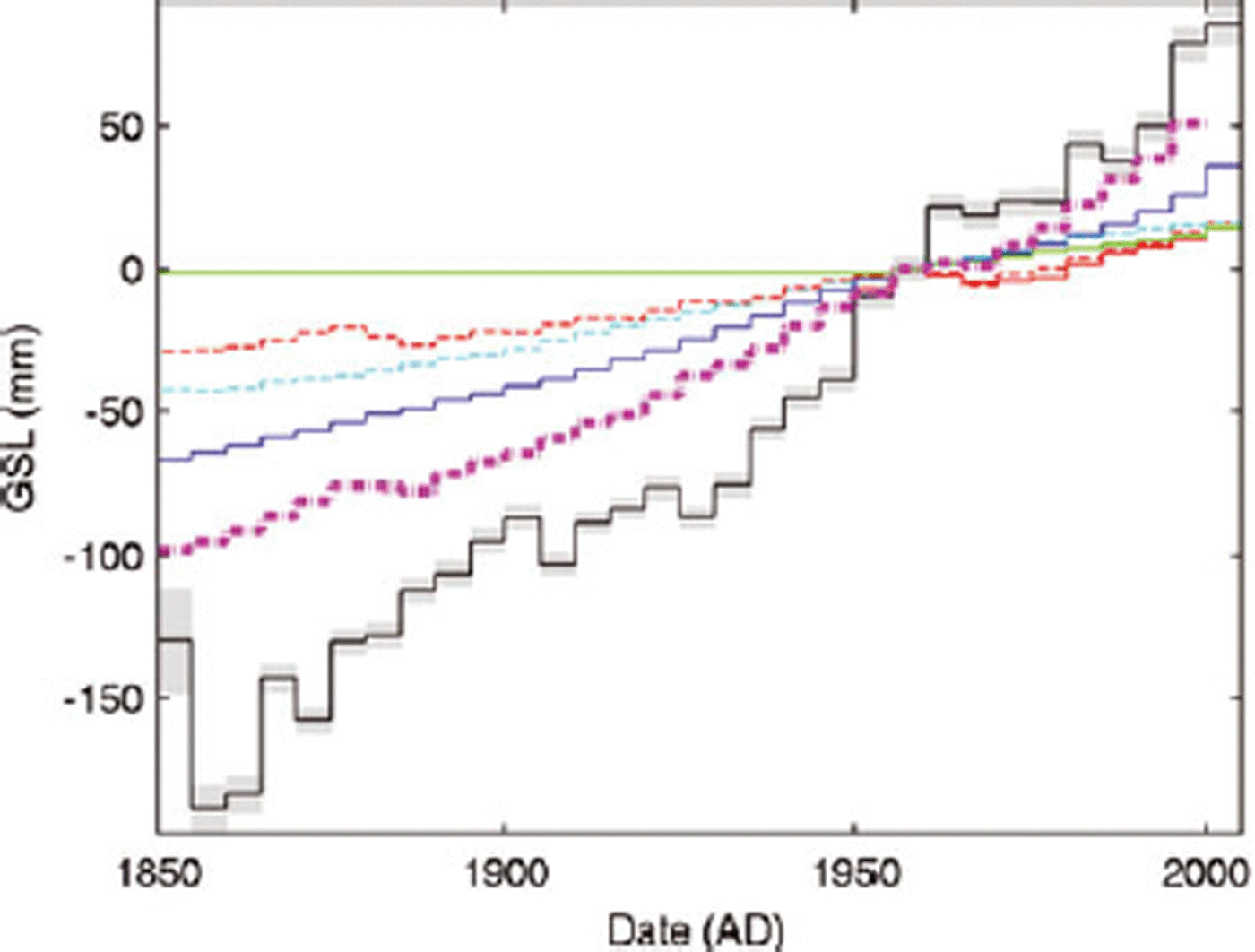
1850–1950 period
In Figure 5 we look at the residuals of GSL since 1850. Perhaps the most noticeable feature, though, is the large, ~45mm jump in GSL residual that occurs between 1950 and 1960. There is no significant trend for the periods 1900–50 or 1955–2005 (Fig. 4) if this almost step change is removed. While this feature may be purely errors in the various components, it is also interesting to note this occurs during a period when TS reaches a local maximum. The step change in residual GSL also corresponds to a period when volcanic activity was very low and the ENSO index is at its most negative during the entire record. Since ENSO activity and heat content are closely related to ocean circulation patterns, the step change may be associated with changing ocean circulation rather than, say, changes in the ice sheets. The 1855–1900 period has a residual that amounts to about the same as the sum of the TS and GSIC components (~35 mm), only accounting for about half the observed sea-level rise (Fig. 2). The generally rising trend from 1850 to 1900 may be a reaction to the termination of the Little Ice Age, when glacier retreat was widespread, and may have included the large ice sheets as well as the smaller high-latitude glaciers. This is hard to estimate with any reasonable modeling at present since temperature data from the high latitudes are very sparse or non-existent in the 19th century.
Modeled thermosteric sea level (red; Reference Gregory, Lowe and TettGregory and others 2006), and residual sea level (thick black line) calculated as GSL-modeled TS–GSIC (Reference CogleyCogley, 2009). SPG, GIS and Antarctic contributions are assumed to be zero throughout. The volcanic component is represented as in Figure 4 by the thin black curve. The blue curve shows 12 month smoothed ENSO (right-hand scale) calculated as in the text.
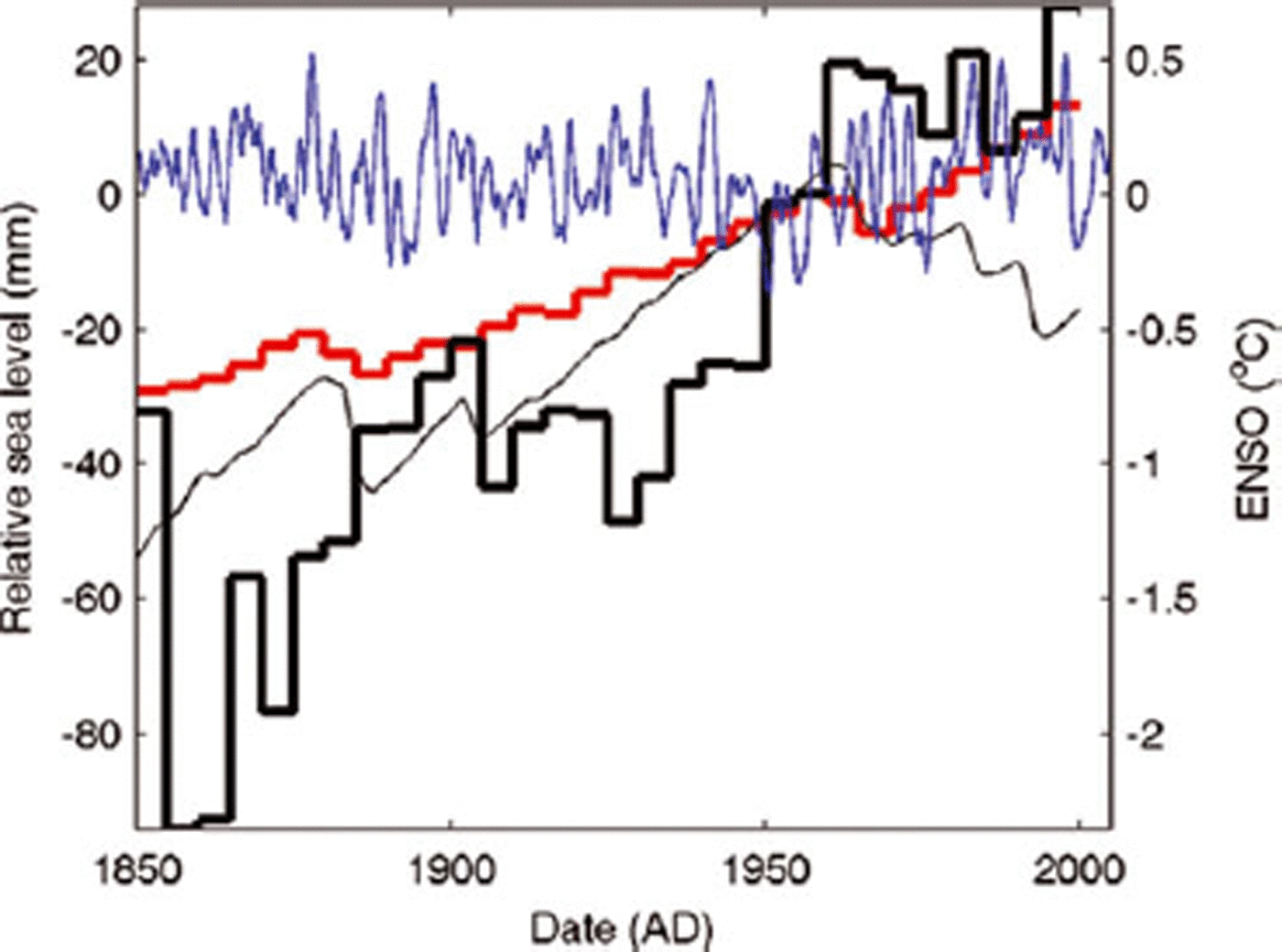
There are highly significant relationships between GSL residual and volcanic forcing of sea level and with ENSO and also North Atlantic Oscillation (NAO, not shown). Thermosteric modeled sea level is significantly affected by volcanic forcing and marginally significantly affected by either ENSO or NAO. Thermosteric sea level is also strongly significantly related to volcanic sea-level variability, and marginally significantly related to ENSO variability.
The amplitude of decadal oscillations in residual GSL is ~20mm since about 1870, a similar amount to the post-1955 residual, some of which is likely due to unaccounted-for melt from both the small polar glaciers and the Greenland ice sheet, though observed rates of increased melting since 2000 are far less than the observed amplitude of fluctuations. This variability suggests that errors are indeed, as expected, much larger pre-1955 in the sea-level budget components.
Uncertainties
Thermosteric sea level
The main source of ocean heat measurements is the set discussed and updated by Reference Levitus, Antonov, Boyer, Locarnini, Garcia and MishonovLevitus and others (2009), though Reference Ishii and KimotoIshii and Kimoto (2009) supplement these with other data. The reduced salinity of the oceans contributing to thermosteric rise is estimated to be much lower than that caused by rising heat content (Reference Ishii, Kimoto, Sakamoto and IwasakiIshii and others, 2006). Widely varying estimates of the rate of increase of GOHC have been derived: for example, linear trends for the 1969–2003 period, when measurements were made mainly by one type of instrument, range from (with 95% confidence intervals) 0.24±0.04 (Reference Ishii and KimotoIshii and Kimoto, 2009) to 0.41±0.06×10²² J a–1 (Reference DominguesDomingues and others, 2008). These differences depend on the method used to produce global rates from the spatially inhomogeneous dataset.
A key element of the steric sea-level rise component is the contribution from the deep ocean below 700m depth. To date, little is known about this component. Reference Antonov, Levitus and BoyerAntonov and others (2005) suggest that steric sea-level rise is ~0.4mma–1, with the deeper ocean contributing only ~0.1mma–1. Reference DominguesDomingues and others (2008) used the approximate ratio of steric sea-level rise for the deeper ocean relative to the upper 700 m to correct their steric sea level derived from the upper 700m alone. But, since their steric sea-level rise was already ~50% larger than earlier estimates (Reference Antonov, Levitus and BoyerAntonov and others, 2005; Reference Levitus, Antonov and BoyerLevitus and others, 2005; Reference Ishii, Kimoto, Sakamoto and IwasakiIshii and others, 2006), Reference DominguesDomingues and others (2008) added a further ~0.2mma–1 for the deeper ocean, resulting in almost a doubling relative to other estimates. This correction may be unsound, as there may be areas where the deep-water contribution is in opposition to the upper part of the water column. Direct estimates of GOHC may well be biased because of large data gaps in the Southern Hemisphere.
Reference DominguesDomingues and others (2008) reconstructed GOHC, and Reference Church and WhiteChurch and White (2006) global mean sea level, using a variant of the optimal interpolation scheme by Reference Kaplan, Kushnir and CaneKaplan and others (2000). The leading empirical orthogonal functions (EOFs) were determined from 12 years (1993–2004) of detrended TOPEX/Poseidon and Jason-1 satellite altimeter data. The principal components of the leading EOFs were then determined in a least-squares manner to fit the tide-gauge observations.
We note that the last 15 years have been exceptionally warm compared with the historical records and that the EOF patterns may not be representative of the patterns prevailing earlier in the century. Reference Kaplan, Kushnir and CaneKaplan and others (2000) caution against using too short a time period for calculating the EOFs: ‘To obtain faithful field reconstructions, we have to use a relatively long time period for the covariance estimation, and there should be enough data in it for estimating all necessary cross covariances.’
Terrestrial water budget
Reference Vermeer and RahmstorfVermeer and Rahmstorf (2010) used the results from Reference Chao, Wu and LiChao and others (2008) to estimate potential contribution from water impoundment in the world artificial reservoirs. However, Reference Chao, Wu and LiChao and others (2008) focused on an estimation of contributions that decrease sea-level rise (storage in reservoirs) only, amounting to about –0.44mma–1. There are, however, several processes that were not considered by Reference Chao, Wu and LiChao and others (2008), and they all lead to higher sea levels. The processes that increase sea level include groundwater mining, estimated as contributing 0.55–0.64mma–1 between 1990 and 1995 by Reference ShiklomanovShiklomanov (1997), and urbanization with a contribution of 0.3 mma–1 (Reference Gornitz, Douglas, Kearney and LeathermanGornitz, 2001). According to Reference SahagianSahagian (2000), the sum of the above effects could be of the order of 0.05 mma–1 sea-level rise over the past 50 years, with an uncertainty several times as large.
In addition, Reference Lettenmaier and MillyLettenmaier and Milly (2009) provide a state-of-the-art estimation of the contributions from continental mass losses/gains: ‘We would find it difficult to refute convincingly, on the basis of observations, the proposition that land, overall, contributes essentially nothing to sea-level rise today’.
However, we suggest that decadal variability in sea level is likely to be associated with variability in global water cycle. Changes of 5% in global river discharge (Reference Fekete, Vörösmarty and GrabsFekete and others, 1999) correspond to 5mma–1 in GSL, similar to changes in GSL associated with El Niño or a large volcanic eruption (Reference Grinsted, Moore and JevrejevaGrinsted and others, 2007). In addition, changes in GOHC influence the hydrological cycle, leading to changes in continental water storage, which partly compensates for thermosteric volume changes (Reference Ngo-Duc, Laval, Polcher, Lombard and CazenaveNgo-Duc and others, 2005; Reference Grinsted, Moore and JevrejevaGrinsted and others, 2007).
Antarctic ice sheet response
Reference Wingham, Shepherd, Muir and MarshallWingham and others (2006) discuss Antarctic mass balance using satellite radar altimetry over the period 1993–2003. They find virtually no significant trend over this time. Estimates based on outflow velocity changes in glaciers using interferometric synthetic aperture radar (InSAR; Reference RignotRignot and others, 2008b) suggest an increase in mass loss, but with very large error bars, from 112±92 Gt a–1 in 1996 to 196±92 Gt a–1 in 2006. Since 2003, Gravity Recovery and Climate Experiment (GRACE) estimates indicate significant mass loss (Reference VelicognaVelicogna, 2009), which taken together with the altimetry and InSAR data (Reference RignotRignot and others, 2008b) suggests accelerating loss of ice. Indeed given a mass loss of 104 Gt a–1 in 2002, 247 Gt a–1 in 2009 and an acceleration of –26 Gt a–2, mass loss would have been zero in 2000, in reasonable agreement with the altimeter and InSAR results. Indeed estimates of negative mass balance from GRACE data rely on the isostatic correction applied to the Antarctic, which Reference VelicognaVelicogna (2009) acknowledges as the largest source of error in the mass-balance estimate. Recent estimates from satellite altimetry seem to contradict GRACE mass loss estimates from Antarctica. The pattern of negative mass balance from West Antarctica and more positive balance from East Antarctica is the same for both methods; however, altimetry estimates suggest that the East Antarctic ice sheet is gaining more mass than is lost by West Antarctica (personal communication from J. Zwally, 2010). Recent combined estimates of land uplift and mass loss (Reference WuWu and others, 2010) suggest that between 2002 and 2008 West Antarctica had a net loss of 99 Gt a–1 while East Antarctica had a net gain of 16 Gt a–1. There is no observational reason to propose that Antarctic mass balance was negative prior to the 1990s; however, we cannot rule out that it was positive earlier in time.
Conclusion
Recent (post-2003) components of the sea-level budget appear in plausible agreement with observations: steric sea level is rising at ~0.6mma–1 (ranging from ~0.05mma–1 (Reference Levitus, Antonov, Boyer, Locarnini, Garcia and MishonovLevitus and others, 2009) to 1.1 mma–1 (Reference von Schuckmann, Galliard and Le Traonvon Schuckmann and others, 2009)). Despite large uncertainties in steric component, the agreement between the modeled TS and that estimated from observations over the 1955–2005 period argues that despite such a wide range in recent estimates, the TS component is reasonably well constrained. Mass contributions from GRACE estimates of ice loss from Greenland and Antarctic ice sheets are ~1.1mma–1 (with uncertainties of ~50% due to the short time period of the GRACE data). Small glaciers and ice caps contribute ~1.3±0.2mma–1. This compares with an observed sea-level rise rate of ~3.3mma–1. Hence the budget is in fair agreement with the observations.
The post-1955 sea-level budget, though measured over longer time intervals, is more open to question: since overall rise rates were lower, the relative magnitude of the errors associated with each component was more significant. The observed sea-level rise rate from tide gauges was ~1.7mma–1 (1955–2000). Glaciological estimates for the mass balance of the ice sheets were based on limited survey methods, and only gained from satellite altimetry from about 1993. A simple addition of measured steric and glacier mass-balance components leads to a significant shortfall in the sea-level budget since 1850. The missing component of the sea-level trend since 1955 contributes ~0.36mma–1. This can, however, be well filled by estimates of mass balance of unsurveyed high-latitude small glaciers and ice caps, predominantly in the Antarctic Peninsula, which are modeled as contributing 0.28 mma–1 (Reference Hock, deWoul, Radiá and DyurgerovHock and others, 2009). The reasonable closure of the 1955–2005 sea-level budget suggests that total terrestrial and extra ice-sheet contributions to sea level beyond those listed in Table 1 are small for the 1955–2005 period. This closure also seems consistent with the only recent observed dynamic changes in central Greenland as it responds to marginal mass wastage (personal communication from Weili Wang, 2010).
Pre-1955 estimates exist for thermosteric and temperate-latitude glaciers and ice caps, though the mass term has much greater errors than for the post-1955 period due to the fewer glaciers measured. However, the sum of these components is also much less than required to close the budget, but much of the difference can be explained by a large mass loss of ~45mm between 1950 and 1960. There is also a trend in the residuals from 1850 to 1900 of ~35mm that is likely a response to the end of the Little Ice Age resulting in glacier wastage. Some of the pentadal variability, and the 1950s step increase may be explained by ENSO and volcanic impacts on ocean heat content, global water cycle and reductions in ice melt.
Acknowledgements
We thank G. Cogley for kindly providing the GSIC 5 year data, L. Wake and an anonymous referee for improving the manuscript, and R. Hock, J. Zwally and Weili Wang for useful discussions. The research was partly funded by NSFC No. 41076125 and China’s National Key Science Program for Global Change Research (No. 2010C8950504).


