


1. Introduction
The interaction of compliant surfaces with wall-bounded flows has been the subject of research over the last decades since the early experiments published by Kramer (Reference Kramer1957, Reference Kramer1962). The main research has been focussed on the application of compliant coatings to delay laminar-to-turbulent transition, reduce frictional drag and suppress flow-induced noise and vibrations.
Theoretical analyses on system instabilities, direct numerical simulations (DNS) and experimental investigations have shown the opportunities and limitations of compliant materials in achieving the aforementioned goals, resulting in a series of contradictions and controversies. A review on classical and more recent studies are given by Bushnell, Hefner & Ash (Reference Bushnell, Hefner and Ash1977), Riley, Gad-el Hak & Metcalfe (Reference Riley, Gad-el Hak and Metcalfe1988) and Gad-el Hak (Reference Gad-el Hak2002), which indicates a valuable direction to the state-of-the-art research on compliant walls.
The present knowledge regarding possible turbulent drag reduction quantifies the compliance of flexible walls as a result of the response to the pressure fluctuations in the turbulent boundary layer. Dominant near-wall flow structures instigate quasi-periodic bursting events and result in velocity fluctuations in the streamwise and wall-normal directions (i.e.  $u'$ and $v'$, respectively), which, when correlated, are the elementary components of the Reynolds shear stress $-\rho \langle u'v' \rangle$ in the turbulent boundary layer with $\rho$ as the fluid density (Tennekes & Lumley Reference Tennekes and Lumley1972; Robinson Reference Robinson1991). The velocity fluctuations contribute to the near-wall pressure fluctuations as is indicated by the conservation of momentum for incompressible flows:
 \begin{equation} \boldsymbol{\nabla}p ={-}\rho \left ( \frac{\partial \boldsymbol{u}}{\partial t}+\left ( \boldsymbol{u}\boldsymbol{\cdot}\boldsymbol{\nabla} \right) \boldsymbol{u} \right )+\mu \nabla^{2}\boldsymbol{u} . \end{equation}
The pressure gradient  $\boldsymbol {\nabla } p$ is related to the velocity fluctuations in time and space, in the absence of external forces. The bursting events in the turbulent boundary layer result in local pressure fluctuations that are able to deform the flexible wall, dependent on the material properties of the compliant layer. Possible reduction of turbulent drag is based on the hypothesis that a compliant surface is triggered by a pre-bursting event and should thereby impede a new burst formation. Favourable wall dynamics in streamwise ( $u_c$) and wall-normal directions ( $v_c$) suppress the related velocity fluctuations $u'$ and $v'$, which might result in lower Reynolds stresses when assuming $-\rho \langle (u'+u_c)(v'+v_c) \rangle$ (Kulik et al. Reference Kulik, Rodyakin, Suh, Lee and Chun2005).
The response of a compliant surface to the pressure fluctuations in a turbulent shear flow was theoretically examined by Duncan (Reference Duncan1986), Chase (Reference Chase1991) and more recently by Benschop et al. (Reference Benschop, Greidanus, Delfos, Westerweel and Breugem2019). The surface response is directly linked to the shear stress and the pressure pulses related to the flow structures in a turbulent boundary layer. Surface instabilities occurred when the ratio between the dynamic pressure of the flow  $p_{rms}$ with respect to the shear modulus of the coating $|G^*|$ exceeded a critical value, which was related to the turbulent flow conditions in combination with coating properties, such as geometry, the size of the fluctuation, coating density and layer thickness (Kulik Reference Kulik2012). Nevertheless, it is still unclear what induces the onset of surface instabilities under turbulent flow conditions.
The flow-induced surface instabilities (FISIs) have been classified into two main types of wave phenomena (Gad-El-Hak, Blackwelder & Riley Reference Gad-El-Hak, Blackwelder and Riley1984; Carpenter & Garrad Reference Carpenter and Garrad1986; Gad-el Hak Reference Gad-el Hak1986), static divergence and wave flutter, both of which move in the streamwise flow direction. Static-divergence waves are damping instabilities due to the viscous properties of the coating material and are slowly moving waves  $U_{wave}\sim 0.05 U_{bulk}$ with very large amplitudes and large wavelengths. Wave flutter is an elastic instability that can be stabilised by damping and the waves propagate much faster $U_{wave} \sim C_t$ with lower amplitudes and shorter wavelengths, where the shear-wave velocity of the compliant material is defined by $C_t=(|G^*|/\rho _c)^{1/2}$ with $|G^*|$ as the shear modulus of the coating and $\rho _c$ as the coating density.
The interaction between turbulent flows and compliant surfaces has also been investigated by several DNS. Often, the wall dynamics is modelled as a mass, damper and spring system, where the wall motions are restricted to the wall-normal direction in most studies. Endo & Himeno (Reference Endo and Himeno2002) observed that the compliant wall moves upwards in the presence of a low-pressure region on the wall and vice versa. They reported a small drag reduction of 2–3 %, whereas minimal changes in the velocity field were observed, although the pressure field was drastically affected. Furthermore, Fukagata et al. (Reference Fukagata, Kern, Chatelain, Koumoutsakos and Kasagi2008) reported a drag reduction of 8 % due to the decrease of the near-wall Reynolds stress forced by the wall motions. However, the turbulent drag increased in a doubled computational domain in the streamwise direction, which was attributed to extensive large wall-normal velocity fluctuations. Kim & Choi (Reference Kim and Choi2014) indicated that very stiff compliant surfaces had minimal effects on the skin-friction drag and the coherent turbulent structures. They showed that soft materials induced large-amplitude waves due to wall resonance, which travelled in the downstream direction. These wall motions increased the fluid motions in the near-wall region significantly. A turbulent boundary layer flow over a compliant surface was also modelled by Xia, Huang & Xu (Reference Xia, Huang and Xu2019) and indicated that the Reynolds shear stress and pressure fluctuation were generally enhanced by the wall compliance for all their cases. Rosti & Brandt (Reference Rosti and Brandt2017) performed numerical simulations of a turbulent channel flow over an incompressible viscous hyper-elastic wall, which was solved with a one-continuum formulation. The turbulent skin friction increased with decreasing elasticity for a fixed bulk Reynolds number  $Re_b$. This result was attributed to the flow being more correlated in the spanwise direction that amplifies the turbulent Reynolds stresses in the fluid, similar to flows over rough and porous walls. An additional DNS study of Rosti & Brandt (Reference Rosti and Brandt2020) indicated a second distinctive mechanism for turbulence production when the bulk Reynolds number $Re_b$ was lowered. At a low Reynolds number, the velocity fluctuations were mainly generated by the small oscillations of the elastic wall that contributed to the turbulent kinetic energy at the fluid–surface interface.
Many experimental studies have been performed on instantaneous wall deformation in relation to wall-bounded flow, which are considered essential for the understanding of the physics of the fluid–surface interaction (Hansen & Hunston Reference Hansen and Hunston1974; Hansen et al. Reference Hansen, Hunston, Ni and Reischman1980; McMichael, Klebanoff & Mease Reference McMichael, Klebanoff and Mease1980; Hansen & Hunston Reference Hansen and Hunston1983; Hess, Peattie & Schwarz Reference Hess, Peattie and Schwarz1993; Lee, Fisher & Schwarz Reference Lee, Fisher and Schwarz1993a,Reference Lee, Fisher and Schwarzb, Reference Lee, Fisher and Schwarz1995; Zhang, Miorini & Katz Reference Zhang, Miorini and Katz2015; Zhang et al. Reference Zhang, Wang, Blake and Katz2017; Huynh & McKeon Reference Huynh and McKeon2020; Wang, Koley & Katz Reference Wang, Koley and Katz2020). Several techniques have been applied to measure the surface deformations and to quantify the flow velocities. Lee et al. (Reference Lee, Fisher and Schwarz1993a) reported the combination of holographic interferometry with laser Doppler velocimetry, whereas Lee et al. (Reference Lee, Fisher and Schwarz1995) used a laser-based electro-optic transducer combined with hot-wire measurements. The latter study also reported a reduction in turbulent activity (i.e. Reynolds stresses).
Non-intrusive diagnostic methods are highly desired to avoid impediment of the surface deformations. Recent studies of Zhang et al. (Reference Zhang, Miorini and Katz2015, Reference Zhang, Wang, Blake and Katz2017) and Wang et al. (Reference Wang, Koley and Katz2020) reported the simultaneous use of Mach–Zehnder interferometry in combination with particle image velocimetry (PIV). For a relative stiff compliant surface, the interaction between the flow and wall deformations was shown to be one-way coupled, where the surface deformations were very small and correlated with the local fluid pressure fluctuations. The wall deformations did not increase the turbulence level of the flow when smaller than one wall unit, although they affected the velocity profile in the viscous sublayer, i.e.  $y^+<5$. Two-way coupling was achieved with a softer compliant wall, where large deformations of the surface changed the turbulent structures in the boundary layer as well (Wang et al. Reference Wang, Koley and Katz2020). Huynh & McKeon (Reference Huynh and McKeon2020) investigated the compliant wall response to the flow structure in a turbulent boundary layer forced by a dynamic roughness element. The combination of 2D-PIV and a stereo digital image correlation (DIC) method was applied to quantify the flow velocity and surface deformations, respectively. The results verified the direct interaction between the forced flow mode and the compliant surface.
A similar mechanism of flow–surface interaction is the wave generation on a liquid surface by a turbulent wind, which was investigated by Paquier, Moisy & Rabaud (Reference Paquier, Moisy and Rabaud2015). The instantaneous surface deformations were measured using the optical method called free-surface synthetic schlieren (Moisy, Rabaud & Salsac Reference Moisy, Rabaud and Salsac2009). The method is based on the analysis of the refracted background image visualised through the liquid/air-interface, similar to the principle of background-oriented schlieren (BOS) (Richard & Raffel Reference Richard and Raffel2001; Raffel Reference Raffel2015). At low wind velocities, the surface deformations were disordered wrinkles with small amplitude, which propagated rapidly in the streamwise direction. The magnitude of the surface amplitude scaled almost linearly with the wind velocity. The wrinkles were considered to be the surface response to the pressure fluctuations travelling in the turbulent boundary layer, which was verified by Perrard et al. (Reference Perrard, Lozano-Durán, Rabaud, Benzaquen and Moisy2019). Above a certain wind velocity threshold a second regime arose, where the liquid–air interface was dominated by well-defined transverse waves propagating in the direction of the wind. The growth rate of the surface amplitude related to the wind velocity was significantly higher than in the first regime. Furthermore, the wave amplitude had a spatial growth in the streamwise direction whereas this was not the case in the wrinkle regime.
The use of compliant surfaces to control the flow conditions passively is a most interesting research topic. The focus of the present work is to investigate and better understand the interaction between a turbulent boundary layer flow and a compliant surface. In particular, the spatial and temporal response of the coating in combination with the change of fluid motions in the near-wall region as a function of the coating properties and the general flow conditions. Special interests are the parametric conditions that force a transition in the coating response. For that purpose, we apply three compliant walls with different material stiffnesses and analyse their surface response to turbulent boundary layer flow. We implement the BOS method similar to Moisy et al. (Reference Moisy, Rabaud and Salsac2009) in order to reconstruct the instantaneous surface deformations. In addition, we also explore the dissimilarities of the velocity profile and turbulence statistics compared with those of a rigid wall. Finally, we elaborate on the opportunities to reduce the turbulent skin friction when applying a compliant surface.
The TU Delft water tunnel facilitate the boundary layer flow experiments over a flat plate, similar to the research of Zverkhovskyi (Reference Zverkhovskyi2014). Three in-house produced compliant coatings with different material properties are embedded in flat test plates, in order to explore the interface wave characteristics as a function of the coating properties and the bulk velocity ( $U_b$). Measurements are taken of (i) the mean skin friction over the total length of the plate using a force balance, (ii) the instantaneous surface deformation field of the coating surface using BOS and (iii) the flow velocity field using 2D PIV/PTV. The outline of this paper is as follows: § 2 discusses the experimental facility, the coating material and the diagnostic methods; the results obtained are discussed in § 3; the main findings are summarised in § 4.
2. Experimental approach
2.1. Water tunnel facility
The experiments have been performed in the water tunnel at the Delft University of Technology figure 1 that was previously used in the investigation by Foeth (Reference Foeth2008). Zverkhovskyi (Reference Zverkhovskyi2014) adapted and utilised the test section to investigate the drag reducing ability of air cavities. The adapted test section is open at the top, which makes it possible to mount test plates in order to determine the frictional properties of various surfaces via a force balance system. The inlet cross-section area is  $300\ {\rm mm}\times 300\ {\rm mm}$, whereas the outlet cross-section area is $300\ {\rm mm}\times 315\ {\rm mm}$ due to an inclined bottom wall. The sloped wall largely compensates for the boundary layer growth in the streamwise direction, such that a nearly constant free stream velocity $U_b$ and zero pressure gradient is maintained. The boundary layer thickness $\delta _{99}$ located at 1.7 m downstream (i.e. region of interest) is characterised as $\delta _{99}=0.057U_b^{-1/7}$. The maximum friction velocity Reynolds number is $Re_\tau =8.3\times 10^3$ at the maximum applied bulk velocity of $5.4\ {\rm m}\ {\rm s}^{-1}$ ( ${\sim }500\ {\rm L} {\rm s}^{-1}$), which corresponds to a similar range as reported by Wang et al. (Reference Wang, Koley and Katz2020). The Reynolds number is defined by $Re_\tau = \delta _{99}u_\tau /\nu$, with the boundary layer thickness $\delta _{99}$, the wall-friction velocity $u_\tau$ and the kinematic viscosity $\nu$. The wall-friction velocity $u_\tau$ is derived from $\tau _w=\rho _f u_\tau ^2$, with $\tau _w$ the determined wall shear stress over a rigid wall and $\rho _f$ the fluid density. The boundary layers at the wall are tripped just before the entrance of the test section to ensure a turbulent boundary layer at all relevant tunnel velocities. The test plates have a total surface area of $1998\ {\rm mm}\times 297\ {\rm mm}$ and have free in-plane movement during the force measurements. The gaps around the test plate (approximately 1.0–1.5 mm) are shielded in order to minimise possible flow disturbances. The test section is fully optically accessible through bottom and side walls, which makes it possible to apply the BOS and PIV measurements.
Schematic illustration of the water tunnel (Zverkhovskyi Reference Zverkhovskyi2014); shape and dimensions not to scale. The flow is from left to right.

2.2. Compliant material
Polydimethylsiloxane (PDMS) has conventionally been applied as compliant viscoelastic material in fluid–surface interaction studies (Hess et al. Reference Hess, Peattie and Schwarz1993; Choi et al. Reference Choi, Yang, Clayton, Glover, Atlar, Semenov and Kulik1997; Colley et al. Reference Colley, Thomas, Carpenter and Cooper1999; Zhang et al. Reference Zhang, Miorini and Katz2015, Reference Zhang, Wang, Blake and Katz2017). Nevertheless, due to a continuous progress of covalent cross-link reactions between polymer chains, PDMS samples experience an ageing process that modifies the mechanical properties of the material (Bandyopadhyay et al. Reference Bandyopadhyay, Henoch, Hrubes, Semenov, Amirov, Kulik, Malyuga, Choi and Escudier2005; Boiko et al. Reference Boiko, Kulik, Chun and Lee2011). Ongoing and future research on the coating-equipped test plates require a viscoelastic material that maintains its mechanical properties over a sufficient period of time.
Compliant material has been produced in-house from a mixture of triblock-copolymer polystyrene-b-(ethylene-co-butylene)-b-styrene (S-EB-S) and mid-block selective paraffin oil. The SEBS (Kraton G-1650E) has a molar mass of  ${\pm }100.000\ {\rm g}\ {\rm mol}^{-1}$ and styrene content of around 29 %. The paraffin oil (Sigma-Aldrich, 18512) has a dynamic viscosity of $110\unicode{x2013}230\ {\rm mPa}\ {\rm s}$ and a density of $0.827\unicode{x2013}0.89\ {\rm g}\ {\rm cm}^{-3}$ at $20\,^\circ {\rm C}$. The styrene endblocks are thermodynamically incompatible with the paraffin oil and group themselves into micelles to minimise interfacial area, which are considered to be the cross-link points in the material. These points are connected by the EB mid-blocks via physical cross-linking and give formation to a three-dimensional network, as illustrated in figure 2. A higher concentration of SEBS increases the micelles and cross-link density, which in part determines the mechanical properties of the viscoelastic material. Other parameters that influence the mechanical properties are the molar mass and the styrene content of the triblock copolymer and the type of hydrocarbon oil (Dürrschmidt & Hoffmann Reference Dürrschmidt and Hoffmann2001; Kim, Paglicawan & Balasubramanian Reference Kim, Paglicawan and Balasubramanian2006; Lattermann & Krekhova Reference Lattermann and Krekhova2006).
SEBS/Oil micelles network formation. (a) Bridges: each styrene endblock colonises in a different micelle. (b) Loops: each styrene endblock colonises in the same micelle. (c) Dangling ends: one styrene endblock remains unsettled. Illustration based on Laurer et al. (Reference Laurer, Mulling, Khan, Spontak and Bukovnik1998).

Three coatings with different material stiffness  $|G^*|$ are obtained by increasing the SEBS concentration. The material properties are characterised on their rheological behaviour using a rheometer (ARES-G2, TA Instruments) with a parallel plate geometry with a diameter of 25 mm. A temperature-sweep procedure estimates the polymer flow temperature $T_m$, which is of great interest for the material post-processing to obtain a smooth coating surface on the test plates. The results confirm the material stiffness $|G^*|$ and the polymer flow temperature $T_m$ increases with increasing SEBS concentration (table 1). The shear wave velocities $C_t = (|G^*|/\rho _c)^{1/2}$ are within the range of the flow velocities of the water tunnel and, thus, surface deformations and/or instabilities are expected. The material is considered to be incompressible within the range of operation (i.e. bulk modulus $K \sim 5\ {\rm GPa}$), which presumes a Poisson's ratio of $\sigma \simeq 0.5$.
Material properties of the three compliant coatings at standard conditions. The frequency-averaged storage modulus  $G'$ and loss modulus $G''$ determine the complex shear modulus $G^*= G'+iG''$ with $|G^*|=\sqrt {(G')^2+(G'')^2}$. The shear wave velocity is given by $C_t = (|G^*|/\rho _c)^{1/2}$.

The refractive index of the coating is required in order to reconstruct the coating deformations at the surface interface. The refractive indices  $n_i$ are measured with an Abbe refractometer and are summarised in table 1.
The coating-equipped test plates are obtained by liquifying and re-solidifying the compliant material using a large oven. This method of material processing delivers a homogeneous coating layer thickness of  $h_c=5$ mm with an interface surface that is considered to be hydrodynamically smooth.
2.3. Surface deformation measurements
The instantaneous deformation field  $\zeta (x,y,t)$ of the compliant surface are measured by the BOS method similar to that of Moisy et al. (Reference Moisy, Rabaud and Salsac2009). A random dot pattern ( $100\ {\rm mm}\times 100\ {\rm mm}$) is used with non-overlapping dots, dot size $D_d\sim 0.4$ mm and a dot density of 40 %. This corresponds to a number of dots $N_I \approx 6$ for a $32 \times 32$ pixels interrogation window and a particle-per-pixel $N_{ppp}\approx 0.125$, leading to more than 90 % of good vectors (Adrian & Westerweel Reference Adrian and Westerweel2011). The random dot pattern is placed behind the coating–fluid interface and was back-illuminated by a homogeneous LED screen. Both are submerged below the free surface of the water above the test plate. The dot pattern is front-observed by a high-speed 4-megapixel camera (Imager HS, LaVision) via a mirror that is placed below the test section (figure 3). A distorted image of the reference dot pattern is the result of light rays passing through the deformed interface. The apparent local displacement of the reference image is computed via an in-house DIC algorithm and is directly proportional to the local surface gradient (Elwell Reference Elwell2005). A multigrid interrogation approach is used with a final window size of $16\times 16$ pixels with a 50 % overlap, leading to a displacement field with a high resolution (i.e. vector/8 pixels). A simple median filter method is applied to detect spurious vectors that are replaced by linear interpolation (Westerweel & Scarano Reference Westerweel and Scarano2005). The final interrogation window is smaller than required for $N_I \approx 6$. However, the computed displacement fields are similar to the correlation with a $32 \times 32$ pixels interrogation window. The reconstruction of the surface interface is further discussed in Appendix A.1.
BOS set-up in order to perform surface deformation measurements. The camera observes the random dot pattern via a mirror and the transparent coating material. The total distance between the camera and the dot pattern is  $H=1400$ mm. The flow moves from left to right.

The refraction method has to fulfil at least two requirements for a reliable reconstruction of the surface deformation, as discussed by Moisy et al. (Reference Moisy, Rabaud and Salsac2009). First, the camera–pattern distance  $H$ needs to be large enough compared with the field size $L$ to meet the paraxial approximation. In the present case, the field of view (FOV) has an area of $100\ {\rm mm}\times 100\ {\rm mm}$ in the centre of the plate and the camera–pattern distance is around $H=1400$ mm thereby satisfying the paraxial approximation, i.e. $\beta \simeq L/(\sqrt {2}H) \ll 1$. Second, the wave amplitude and surface curvature need to be small to fulfil the linear approximation. The DIC algorithm is inferior when strong surface deformations occur; strong strained refracted patterns or dots that move in opposite directions within one interrogation window will result in bad displacement vectors. A dot-tracking algorithm (DTA) would be more appropriate when strong deformations occur; see Charruault et al. (Reference Charruault, Greidanus, Breugem and Westerweel2018). The pattern–surface distance is minimal 15 mm and could be increased by inserting glass spacer plates of various thicknesses $h_g=2$, 10 or 20 mm. An increase in pattern–surface distance amplifies the deformations and with that the resolution. However, it may also lead to ray crossing in regions of large strain resulting in inaccurate displacement values preventing an unambiguous reconstruction of the coating surface.
2.4. Flow velocity measurements
Particle image velocimetry is used to study the instantaneous velocity fields and turbulent statistics of the turbulent flow. A standard 2D-2C PIV configuration is applied to the test facility, as is displayed in figure 4. The FOV is around  $8.7\times 7.0\ {\rm mm}^2$ in streamwise and wall-normal direction, respectively, and is situated 1.7 m downstream from the entrance of the test section. The FOV is illuminated by a light sheet $\Delta z_0<1$ mm using a double-pulsed 50 mW Nd:YAG laser (Litron L-class 50-50) and is located in the centre of the tunnel. The images are recorded by a $1280\times 1024$ pixel CCD camera (FlowMaster, LaVision) and show a part of the wall and the near-wall flow region. Hollow glass particles (Sphericell, $d_p = 10\ \mathrm {\mu }{\rm m}$) are used as tracers, with a nominal particle density of approximately $\rho _d = 1.1\times 10^3\ {\rm kg}\ {\rm m}^{-3}$. The response timescale of particle relaxation $\tau _p=d_p^2 \rho _p/(18\rho _f \nu )$ is $5.6\ \mathrm {\mu }{\rm s}$. The particles are expected to follow the flow even in the near-wall region as the expected inner turbulence timescale is minimally ${\tau _\nu =\nu /u_\tau ^2>20\ \mathrm {\mu }{\rm s}}$. Calibration is done using a calibration grid with a dot spacing of 0.5 mm. The pixel size is $6.7\ \mathrm {\mu }{\rm m}$, resulting in a $M_0=1$ magnification. A total of 500 successive PIV image pairs are taken at a low frequency (3–4 Hz) to ensure reliable statistical convergence of the mean velocity field and turbulent parameters. The time delay $\Delta t$ between the first and second image is chosen such that the particle displacement between the two images is around 8–10 pixels from the wall. Data analysis is performed using commercial software (DaVis v7, LaVison). A multi-pass correlation is used, with a final interrogation window size of $64 \times 64$ pixels with a 75 % overlap resulting in a vector spacing of 0.11 mm. The final $64\times 64$ pixels window is the minimum size to satisfy the criterion of at least five particles per interrogation window.
Illustration of the experimental PIV set-up applied to the test section of the facility. The FOV is located 1.7 m downstream from the entrance of the test section and at the centreline of the water tunnel. The flow moves from left to right.

Close to the wall, the velocity profiles show relatively low spatial resolution due to the large interrogation window. The corresponding vector spacing is 7–20 wall units ( $y^+$) for bulk velocities $U_b= 1.7 \unicode{x2013} 5.2\ {\rm m}\ {\rm s}^{-1}$ ( $Re_\tau =3.3\times 10^3\unicode{x2013}8.0\times 10^3$), respectively. The reconstruction of the velocity profile closer to the wall requires a higher spatial resolution and is obtained by applying particle tracking velocimetry (PTV), which determines the displacement of individual particle images close to the wall ( $y<1$ mm). The spatial resolution of the mean velocity profile is enhanced up to 1 pixel, by means of the so-called super-resolution method (Keane, Adrian & Zhang Reference Keane, Adrian and Zhang1995). First, an in-house PIV correlation algorithm with elongated interrogation windows ( ${\sim }64\ {\rm pixels}\times 32\ {\rm pixels}$, 50 % overlap) is used that provides identical results as the earlier used commercial software. Second, the measured estimate of the local velocity field is used as an input for the PTV processing, thus improving the successful and fast detection of particle pairs by substantially reducing the search area. The particle image displacement between two successive images with $\Delta t$ in between results in the velocity of all individual particles. The mean velocity profile is obtained by spatial and temporal averaging of the particle velocities with respect to the mean position of the compliant wall.
3. Results and discussion
3.1. Friction force measurements
The measured friction force  $\bar {F}$ represents the averaged shear stress $\bar {\tau }$ times the total test plate area $A$, such that $\bar {\tau }=\bar {F}/A$. Figure 5(a) shows the averaged shear stress $\bar {\tau }$ against the bulk velocity $U_b$. Following Zverkhovskyi (Reference Zverkhovskyi2014), the results are highly reproducible and are compared with two common smooth-surface curves, the Grigson and the Prandtl–Schlichting correlation curves. For low bulk velocities, the friction values of all three coatings are similar to those of a rigid smooth surface. Above a bulk velocity of $U_b>4.5\ {\rm m}\ {\rm s}^{-1}$ or $Re_\tau >7.1\times 10^3$, the shear stress of coating 1 deviates more and more with increasing bulk velocity $U_b$. Coatings 2 and 3 maintain their smooth surface behaviour up to the maximum applied bulk velocity.
(a) Wall shear stress  $\bar {\tau }$ as a function of water tunnel bulk velocity $U_b$. Coating 1 (see table 1) deviates from the estimated correlation lines of Grigson and Prandtl–Schlichting at $U_b=4.5\ {\rm m}\ {\rm s}^{-1}$ and above. (b) Estimated surface roughness $k_s$ related to the measured drag coefficient $C_d$. The dot/dashed line represents the viscous sublayer thickness $\delta _v= 5 \nu /u_\tau$, based on Grigson's correlation.

The coatings are considered to be sensitive to pressure forces, which induce surface irregularities and deformations. The most sensitive surface is coating 1 due to its low shear modulus  $|G^*|$. For coating 1, the measured increase of shear stress $\bar {\tau }$ is presumed to be the consequence of a transition to surface roughness caused by the surface deformations. An estimation of the surface roughness values $k_s$ is obtained by using the drag coefficients $C_d=\bar {\tau }/(\frac {1}{2}\rho U_b^2)$ in combination with the flat-plate friction diagram (White Reference White1999). Below $U_b\sim 4.5\ {\rm m}\ {\rm s}^{-1}$, the coating plate is considered as hydrodynamically smooth, which typically indicates a surface roughness of $k_s^+<5$. As shown in figure 5(b), beyond $U_b=4.5\ {\rm m}\ {\rm s}^{-1}$ the effective surface roughness increases from $k_s=40\ \mathrm {\mu }{\rm m}$ to $130\ \mathrm {\mu }{\rm m}$ (i.e. $k_s^+=6$ to 27).
3.2. Surface reconstruction
3.2.1. Global results and deformation scaling
For all cases, a total of 2000 consecutive height fields  $\zeta (x,y,t)$ are used to analyse the interaction of the turbulent boundary layer with the compliant wall. The root-mean-square (r.m.s.) value of the surface height $\zeta _{rms}$ increases with increasing bulk velocity $U_b$ (figure 6a). For coating 1, an obvious sharp transition is observed around $U_b=4.5\ {\rm m}\ {\rm s}^{-1}$ (or $Re_\tau =7.1\times 10^3$), beyond which the r.m.s. values grow considerably faster. This supports the argumentation that the exceptional frictional increase, as observed in the force measurements (see figure 5a), is due to an increase in the surface roughness related to growing waves with significant amplitudes.
Vertical displacement of coatings 1, 2 and 3. (a) Root-mean-square values  $\zeta _{rms}$ as a function of the bulk velocity $U_b$. The estimated one-way/two-way regime transition of coating 1 occurs when the surface deformation is around $\zeta _{rms}>\delta _v/2$. (b) Scaled r.m.s. values $\zeta _{rms}$ to coating thickness $h_c$ in relation to the scaled pressure fluctuations $p_{rms}$ to coating shear modulus $|G^*|$. The scaling factor 0.0364 of the one-way coupled regime is a fit parameter.

Several authors pointed out the dominant near-wall flow structures to cause pressure fluctuation in the turbulent boundary layer (Tennekes & Lumley Reference Tennekes and Lumley1972; Duncan, Waxman & Tulin Reference Duncan, Waxman and Tulin1985; Robinson Reference Robinson1991). In their turn, the pressure fluctuations are capable of deforming the compliant surface of the wall. Benschop et al. (Reference Benschop, Greidanus, Delfos, Westerweel and Breugem2019) demonstrated the surface deformation of the present coatings using an analytical one-way coupling approach. It was indicated that the shear stress has marginal influence on the vertical displacement and is mainly driven by the pressure fluctuations, which has also been concluded by Perrard et al. (Reference Perrard, Lozano-Durán, Rabaud, Benzaquen and Moisy2019) and Wang et al. (Reference Wang, Koley and Katz2020). The surface-pressure fluctuation level  $p_{rms}$ is estimated, based on the empirical model of the pressure spectrum by Goody (Reference Goody2002, Reference Goody2004). The empirical relation of the surface-pressure fluctuation level $p_{rms}$ is given by Benschop et al. (Reference Benschop, Greidanus, Delfos, Westerweel and Breugem2019)
 \begin{equation} \frac{p_{rms}^2}{\tau_w^2}=0.0309+0.745(\ln(R_T))^2 , \end{equation}
where  $R_T$ is the ratio of the outer layer to inner layer timescales: $R_T=(\delta _{99}/U_b)/(\nu /u_\tau ^2)$. Here we use the boundary layer thickness $\delta _{99}$ and the wall-friction velocity $u_{\tau }$ at a streamwise position $x=1.7$ m, where $u_\tau$ is estimated based on the shear stress values $\tau _{\kappa }$ of table 2. It should be noted that the $p_{rms}$ values slightly deviate compared with the values presented by Benschop et al. (Reference Benschop, Greidanus, Delfos, Westerweel and Breugem2019), where $u_\tau$ is based on 6/7 $\bar {\tau }$. The present results show that the vertical displacement of all coatings scale to $p_{rms}/|G^*|$ and collapse on a single line in the one-way coupled regime (figure 6b). This indicates that the turbulent flow and the related surface-pressure fluctuations $p_{rms}$ deform the compliant coating in proportion to the inverse of the coating stiffness (i.e. $1/|G^*|$). The force measurements indicate that the surface deformations have a negligible effect on the turbulent flow, showing that this is an one-way coupled regime. As can be seen in figure 6(b), coating 1 deviates from the initial line beyond $p_{rms}/|G^*|>0.076$. This is considered as the two-way coupled regime for coating 1, where the surface deformation affects the turbulent flow. The estimated one-way/two-way regime transition of coating 1 occurs when $\zeta _{rms}>\delta _v/2$. Based on this criterion, the transition towards a two-way coupled regime for coating 2 and coating 3 is predicted to be around $U_b=6.8\ {\rm m}\ {\rm s}^{-1}$ (i.e. $p_{rms}/|G^*|\sim 0.045$) and $U_b=9.9\ {\rm m}\ {\rm s}^{-1}$ (i.e. $p_{rms}/|G^*|\sim 0.042$), respectively, although this is still a premature conclusion due to insufficient amount of data in this regime.
Estimated local shear stress via the force measurements ( $\tau _{\bar {\tau }}$) and the log-fit method ( $\tau _\kappa$) for the smooth flat plate and the coated plate, as a function of the bulk velocity $U_b$.

3.3. Surface pattern dependency on the flow conditions
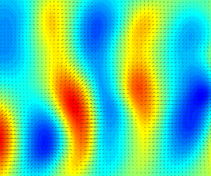
Figure 7 presents six instantaneous height fields  $\zeta (x,y,t)$ of coating 1 with increasing bulk velocity $U_b$ from $0.9\ {\rm m}\ {\rm s}^{-1}$ to $5.0\ {\rm m}\ {\rm s}^{-1}$, which corresponds to $Re_\tau =2.0\times 10^3\unicode{x2013}7.8\times 10^3$. The time series movies of the surface deformation at the related bulk velocities are available in the supplementary material (online). The time series show that the deformations move in the same direction as the fluid flow (i.e. from left to right). At low bulk velocities, the surface deformations exhibit elongated patterns in streamwise direction (figure 7a; movie 1). The wave amplitudes grow with increasing bulk velocity, while the deformation pattern becomes more random-oriented (figures 7b and 7c; movies 2 and 3). Positive surface undulations (crests) $\zeta _c>0$ are usually preceded and/or succeeded by comparably dimensioned valleys $\zeta _v<0$, which is attributed to the incompressibility of the coating material. At the transition velocity $U_b=4.5\ {\rm m}\ {\rm s}^{-1}$, the random-oriented pattern is maintained in combination with incidentally appearing wave packets with much larger amplitudes ( ${\pm }100\ \mathrm {\mu }{\rm m}$), where the wave crests are more oriented in spanwise direction (figure 7d; movie 4). The change in surface pattern orientation with increasing bulk velocity is in agreement with the DNS results of Rosti & Brandt (Reference Rosti and Brandt2017) and the experimental results of Wang et al. (Reference Wang, Koley and Katz2020). Beyond the transition velocity $U_b>4.5\ {\rm m}\ {\rm s}^{-1}$, the surface deformations grow considerably larger than before, and the wave trains start to dominate the surface height field (figure 7e and 7f; movies 5 and 6). The time series of the surface height fields $\zeta (x,y,t)$ show that the wave trains are occasionally overtaken by waves with smaller amplitudes, which indicates that two types of waves exist that are travelling in the streamwise direction on the fluid–surface interface with different wave dynamics. The r.m.s. value of the surface height field $\zeta _{rms}$ (figure 6, coating 1) shows the sharp transition in amplitude growth with increasing bulk velocity $U_b$. This is due to the increase in wave height as well as the increase in the percentage of surface area covered by these high-amplitude waves, as shown in figure 8. This is also visualised and supported by the instantaneous height fields $\zeta (x,y,t)$.
Instantaneous surface height fields  $\zeta (x,y)$ of coating 1 with increasing flow velocity $U_b$. The flow moves from left to right. The colour scales vary for the different bulk velocities. The time series movies of the surface deformation are available in the supplementary material (online) available at https://doi.org/10.1017/jfm.2022.774.

(a) Percentage of surface area (coating 1) that is covered with waves where the absolute value of the crest  $|\zeta _c|$ or the valley $|\zeta _v|$ is respectively higher or lower than the viscous boundary layer $\delta _v$. The dotted line represents the data-fitted sigmoid curve. (b) Table presenting the viscous boundary layer thickness $\delta _v$, the coating surface fluctuation $\zeta _{rms}$ (coating 1) and the percentage of $|\zeta _c|,|\zeta _v|>\delta _v$ related to the flow conditions.

The height fields  $\zeta (x,y,t)$ of coatings 2 and 3 (not shown) maintain the random-oriented surface pattern with increasing bulk velocity $U_b$ up to the maximum bulk velocity in this study. Seemingly, the deformation pattern with the accompanying undulations reduces in size, whereas the wave amplitudes increase with increasing bulk velocity. A more quantitative analysis of the pattern dimensions and wave dynamics is discussed in §§ 3.4 and 3.5, respectively.
3.4. Spatial correlation
The spatial structure of the surface wave is characterised by using the 2D two-point spatial correlation coefficient of the surface height field  $C(r_x,r_y)$, which is defined as
 \begin{equation} C(r_x,r_y)=\frac{\left \langle \zeta(x,y,t) \cdot \zeta(x+r_x,y+r_y,t) \right \rangle}{\left \langle \zeta(x,y,t)^2 \right \rangle}. \end{equation}
 The  $xy$-correlation maps of coating 1 can be found in Appendix A.3.1. The characteristic wavelength $\lambda _x$ in streamwise direction is estimated by analysing the correlation function, where the correlation coefficient equals $C(r_x,r_y)=C(\lambda _x/6,0)=0.5$. Likewise, the characteristic wave width $\lambda _y$ in spanwise direction is determined by $C(r_x,r_y)=C(0,\lambda _y/6)=0.5$. Figure 9 shows the estimated length scales $\lambda _x$ and $\lambda _y$ of the surface deformation of coatings 1, 2 and 3 in relation to the bulk velocity $U_b$. Initially, coating 1 shows a reduction of the wavelength $\lambda _x$ at very low bulk velocities down to $\lambda _x\sim 15$ mm around $U_b=2.0\unicode{x2013}2.5 \ {\rm m}\ {\rm s}^{-1}$. This equals the wavelength of the predicted peak response with $\lambda _x=3h_c$, as reported by Kulik, Lee & Chun (Reference Kulik, Lee and Chun2008), Zhang et al. (Reference Zhang, Wang, Blake and Katz2017) and Benschop et al. (Reference Benschop, Greidanus, Delfos, Westerweel and Breugem2019). When the flow velocity increases, the wavelength $\lambda _x$ grows linearly up to $U_b=4.5\ {\rm m}\ {\rm s}^{-1}$, from where a rapid transition occurs of the wavelength $\lambda _x$ decreasing again to a wavelength value around $\lambda _x \sim 11$ mm. The characteristic wavelength $\lambda _x$ of coatings 2 and 3 decreases with increasing bulk velocity, however, the minimum wavelength of coating 2 seems to be restricted to $\lambda _x\sim 15$ mm at high flow velocities (i.e. $\lambda _x/h_c\sim 3$). Regarding the wave width, coating 1 has $\lambda _y$ values around $20\unicode{x2013}25$ mm before the rapid transition of surface deformation, after which the value quickly increases to $\lambda _y \sim 33$ mm. This confirms that the surface deformation pattern and the shape of pre- and post-transition waves are very different. Coatings 2 and 3 show a decreasing wave width $\lambda _y$ with increasing bulk flow velocities.
(a) Streamwise  $\lambda _x$ and (b) spanwise $\lambda _y$ length scales versus bulk velocity $U_b$.

Figure 10 presents the scaled characteristic wave parameters  $\lambda _x/h_c$ and $\lambda _y/h_c$ in relation to the estimated dominant pressure fluctuations over the coating stiffness, i.e. $p_{rms}/|G^*|$. In the first part $p_{rms}/|G^*|<0.01$, the results of coating 1, 2 and 3 collapse on a single curve, where the wavelength $\lambda _x/h_c$ decreases with increasing flow velocity. This is identical to the phenomenon where the sizes of the flow structures decrease with increasing Reynolds number $Re_\tau$, such that $\lambda _x \propto Re_\tau ^{-1}$. This has previously been reported by Perrard et al. (Reference Perrard, Lozano-Durán, Rabaud, Benzaquen and Moisy2019) in the study on the effect of turbulent wind on a liquid surface. Similarly, the nearly isotropic surface pattern is suggested to be created by the cores of the vortices acting on the compliant wall. Nevertheless, figure 10(a) indicates that the values start to deflect from the initial line beyond $p_{rms}/|G^*|>0.01$, suggesting a different type of coating response to the turbulent flow. This is further discussed in § 3.5.
(a) Streamwise  $\lambda _x/h_c$ and (b) spanwise $\lambda _y/h_c$ length scales versus $p_{rms}/|G^*|$.

3.5. Spatiotemporal correlation
Height–time diagrams for three flow conditions (coating 1) are visualised in figure 11, namely for bulk velocities  $U_b=3.5$, $4.5$ and $5.4\ {\rm m}\ {\rm s}^{-1}$. The height-time diagrams are compiled by plotting a narrow strip of the surface deformation $\zeta (x,y,t)$ in the streamwise direction into the $(x,t)$-plane, resulting in the surface deformation $\zeta (x,t)$ along the middle of the plate. Before the transition at $U_b<4.5\ {\rm m}\ {\rm s}^{-1}$ (figure 11a), one type of surface undulations propagate over the interface in streamwise direction. Around the transition velocity, shorter line segments of high amplitude propagate at a considerably lower velocity (figure 11b). These wave packets become more dominant for the higher bulk velocities. It is observed in figure 11(c) that these slow-moving wave packets are bounded by fast-moving low-amplitude waves, which have a propagation velocity similar as the travelling velocity of the coherent flow structures.
Height–time diagrams of the surface deformation  $\zeta (x,t)$ along the middle of the plate in streamwise direction, for bulk velocities (a) $U_b=3.5\ {\rm m}\ {\rm s}^{-1}$, (b) $U_b=4.5\ {\rm m}\ {\rm s}^{-1}$ and (c) $U_b=5.4\ {\rm m}\ {\rm s}^{-1}$.

The analysis of the spatiotemporal correlation of the surface deformation  $\zeta (x,y,t)$ makes it possible to determine the characteristic propagation velocity of the surface wave $c_w$ in relation to the flow conditions. The spatiotemporal correlation $C(r_x,\tau )$ is the spatially and temporally averaged two-time two-point correlation of the surface deformation $\zeta (x,y,t)$:
 \begin{equation} C(r_x,\tau)=\frac{\left \langle \zeta(x,y,t) \cdot \zeta(x+r_x,y,t+\tau) \right \rangle}{\left \langle \zeta(x,y,t)^2 \right \rangle} . \end{equation}
 The spatiotemporal correlation maps of coating 1 can be found in Appendix A.3.2. In general, the velocity of the propagating waves increases linearly with the bulk velocity, such that  $c_{w_1}=0.7\unicode{x2013}0.8U_b$ (figure 12). This corresponds to the propagation velocity of the highest-intensity turbulent pressure fluctuations high up in the turbulent boundary layer far away from the wall (Willmarth Reference Willmarth1975), which indicates that the pressure fluctuations are responsible for the present surface deformation. Wang et al. (Reference Wang, Koley and Katz2020) reported slightly lower phase velocity of the travelling waves, namely 0.66 $U_b$. However, the spectral peak of their wavenumber–frequency spectra shifts with increasing bulk velocity to $k_x-\omega$ values where the advection velocity of the waves is around $0.7\unicode{x2013}0.8U_b$, in agreement with our results.
Propagation velocity of the surface wave  $c_w/U_b$ of coating 1, 2 and 3 as a function of the bulk velocity $U_b$.

For coating 1, the transition to shorter waves with higher amplitudes modifies the corresponding correlation map of  $U_b=4.5\ {\rm m}\ {\rm s}^{-1}$; small wiggles appear around the local maximum of the correlation values. The wave packets start to dominate the coating–fluid interface. The propagation velocity of these waves is significantly lower than the primary waves before transition, namely $c_{w_2}\sim 17\,\%$ of $U_b$. In this velocity regime $U_b>4.5\ {\rm m}\ {\rm s}^{-1}$, the travelling waves on the surface of coating 2 and 3 maintain the propagation velocity similar to the pressure fluctuations of the flow, namely 70–80 % of $U_b$.
The point of deflection of the initial line in figure 10(a) starts around  $p_{rms}/|G^*|\sim 0.01$ that incidentally corresponds with $c_w/C_t\sim 1$ (figure 13a), i.e. the propagation velocity of the surface waves equals the shear wave velocity of the coating materials. This is in agreement with the theoretical work by Duncan (Reference Duncan1986), where the response of a viscoelastic coating to the pressure fluctuations in a turbulent boundary layer changes at $U_b/C_t\sim 1.2$. The coating response in this next regime is still considered to be stable, where the wavelength increases with increasing flow velocity; very similar to the surface response of coating 1 in the current study. At $c_w/C_t\sim 1$, the characteristic wavelength equals $\lambda _x \approx 3h_c$ and grows with increasing flow velocity up to $\lambda _x \approx 4h_c$ at $c_w/C_t\sim 2.6$ (i.e. at $U_b=4.5\ {\rm m}\ {\rm s}^{-1}$).
(a) Scaled propagation velocity of surface wave  $c_w/C_t$ of coatings 1, 2 and 3 as a function of the scaled wavelength $\lambda _x/h_c$. (b) Scaled wave frequency of coatings 1, 2 and 3 as a function of the normalised flow velocity $U_b/C_t$.

The transition at  $c_w/C_t\sim 2.6$ corresponds with $U_b/C_t\sim 3.4$, which is close to the onset of phase-lag instability reported by Duncan (Reference Duncan1986), namely at $U_b/C_t\sim 2.9$. This destabilisation is caused by the phase difference between the pressure pulses of the flow and the coating deformation in combination with the effect of the upward surface undulations that start to protrude through the viscous sublayer. The combination allows the flow to transfer sufficient energy into the coating layer, which eventually dominates the internal dissipation of the coating layer. This initiates a surface wave with high amplitude that is defined by the nonlinear behaviour of the coating material. Figure 13(b) shows that the related wave frequency $f_w$ in this regime is half of the frequency prior to transition, i.e. $f_{w_2}\approx f_{w_1}/2$, suggesting a second mode of oscillation. Furthermore, the initial part of the graph $U_b/C_t<1.2$ indicates that the coating response frequency depends only on the ratio of the flow conditions $U_b$ and the coating property $C_t$, which is similar to the dependency of the wavelength $\lambda _x$ on $p_{rms}/|G^*|$ observed in figure 10.
To summarise, the global results show that coating 1 experiences an extraordinary interaction with the turbulent boundary layer in comparison with coatings 2 and 3. First, the absolute vertical surface displacement  $\zeta$ is significantly larger at low bulk velocities ( $U_b<4.5\ {\rm m}\ {\rm s}^{-1}$), owing to the coating softness ( ${\sim }1/|G^*|$). Second, coating 1 deals with a rapid transition from which the waves grow considerably with increasing bulk velocity $U_b$, resulting in an unusual dynamic surface roughness that increases the skin friction and turbulent activity. For these reasons, coating 1 has been selected for further consideration within this study regarding the velocity field analysis in order to investigate the interaction between the fluid flow and the compliant surface into more detail.
3.6. Velocity field analysis
This section discusses the analysis of the PIV and PTV measurements. The measurements with the smooth flat plate are compared with those of the coated plate at five bulk velocities: three pre-transition velocities ( $U_b=1.7$, $3.5$ and $4.4\ {\rm m}\ {\rm s}^{-1}$) and two post-transition velocities ( $U_b=4.8$ and $5.2\ {\rm m}\ {\rm s}^{-1}$). As mentioned, only coating 1 is selected for further analysis and to study the interaction between the fluid flow and the compliant surface. The velocity data are obtained by PIV, as well by PTV for the region close to the wall. The instantaneous velocity data is used to determine the mean velocity profiles and to investigate the turbulent flow statistics.
3.6.1. Mean flow analysis
The PIV analysis is used to reconstruct the velocity profile in the log layer, whereas PTV analysis (i.e. super-resolution method Keane et al. Reference Keane, Adrian and Zhang1995) determines the velocity profile in the region close to the wall up to the first part of the log layer. The mean velocity profiles  $\bar {u}$ are obtained by temporally and spatially averaging the velocity fields. Time-averaging is done over 500 instantaneous velocity fields and spatial averaging is applied in the streamwise direction, as the flow is considered to be homogeneous in the streamwise direction given the small FOV. The mean streamwise velocity profiles are presented in figures 14 and 15, where $\bar {u}$ and $y$ are scaled in wall units. The local friction velocity $u_\tau$ is determined by fitting the velocity in the log region with a fixed slope $\partial \bar {u}^+/\partial y^+=1/\kappa y^+$ (Clauser Reference Clauser1956), where $\bar {u}^+=\bar {u}/u_\tau$, $y^+=yu_\tau /\nu$ and $\kappa =0.41$ (Tennekes & Lumley Reference Tennekes and Lumley1972). Although this results in a forced collapse of the velocity data onto the universal log-law line, the application is considered to be valid for high Reynolds numbers (Wei, Schmidt & McMurtry Reference Wei, Schmidt and McMurtry2005). Consequently, the local wall shear stress becomes $\tau _w=\rho _f u_\tau ^2$ and agrees very well with the initially estimated value of $6/7\bar {\tau }_w$ as for a generic developing boundary layer, where $\bar {\tau }_w$ is the averaged wall shear stress obtained by the force measurements. For bulk velocities $U_b<4.5\ {\rm m}\ {\rm s}^{-1}$ (i.e. $U_b/C_t<3.4$), the differences in local shear stresses $\tau _\kappa$ between the coating plate and the smooth plate are slightly larger, as compared with the differences between those values obtained by the force measurements (table 2). This demonstrates that the global force measurements do not perceive a drag change in this regime regarding the coating plate, whereas the results of the local PIV measurements indicate small changes of the frictional drag of 5–10 %.
Pre-transition velocity profiles for the smooth flat plate and coated plate at bulk velocity  $U_b=1.7$, 3.5 and $4.4\ {\rm m}\ {\rm s}^{-1}$, respectively. The surface fluctuation $\zeta _{rms}$ of the coated plate is $0.03\delta _v$, $0.20\delta _v$ and $0.38\delta _v$ for bulk velocity $U_b=1.7$, 3.5 and $4.4\ {\rm m}\ {\rm s}^{-1}$, respectively. The red arrows represent the shift of the high-velocity gradients away from the wall.

Post-transition velocity profiles for the smooth flat plate and coated plate at bulk velocity  $U_b=4.8$ and $5.2\ {\rm m}\ {\rm s}^{-1}$, respectively. The surface fluctuation $\zeta _{rms}$ of the coated plate is $1.5\delta _v$ and $2.7\delta _v$ for bulk velocity $U_b=4.8$ and $5.2\ {\rm m}\ {\rm s}^{-1}$, respectively. The red arrows represent the shift of the high-velocity gradients away from the wall, whereas the black arrows indicate the downwards shift in the log region.

The reconstructed velocity profiles (PTV/PIV) are compared with the theoretical velocity profile related to a smooth flat surface. As expected, the velocity profile of the rigid flat plate matches very well with the theoretical profile for smooth surfaces. The velocity profile at high bulk velocities deviates slightly from the expected profile below  $y^+<10$, most likely due to insufficient amount of particles to properly reconstruct accurate velocities in the near-wall region. In the log-law region $y^+>30$, the velocity profiles show similarity and identical behaviour. The logarithmic relation of smooth walls in the region $y^+>30$ is given by
 \begin{equation} u^+=\frac{1}{\kappa} \ln \left(y^+ \right)+B \end{equation}
with the von Kármán constant  $\kappa = 0.41$ and the smooth-wall log-law intercept $B =5.2$ (Pope Reference Pope2001).
The fluid–surface interaction in the pre-transition regime (figure 14) is considered to be a one-way coupled system, where the turbulent flow initiates moderate deformation of the coating surface, whereas the fluid flow itself is minimally affected. However, the velocity profiles of the flow over the coated plate deviate in the near-wall region due to the small surface deformations. High-velocity gradients in the buffer layer (i.e. at  $y^+\sim 15\unicode{x2013}20$) are visible even at a bulk velocity $U_b=1.7\ {\rm m}\ {\rm s}^{-1}$ with $\zeta _{rms}=0.03\delta _v$, which indicates a low level of two-way coupling. This corresponds to the observations of Wang et al. (Reference Wang, Koley and Katz2020), where the small deformation amplitude $\zeta _{rms}=0.02\delta _v$ at their lowest flow velocity modified the characteristic velocity profile. This low level of two-way coupling has also been reported by Duncan (Reference Duncan1986), where the surface response was considered to be stable. He stated that the maximum surface amplitude has the ability to induce interaction between the coating and the turbulent flow when the flow velocity is $1.2< U_b/C_t<2.9$, which is in close agreement with the current pre-transition regime $U_b/C_t<3.4$. Further away from the wall in the log region, the velocity profiles are unchanged in comparison with the velocity profiles of the smooth flat plate.
For the cases with flow velocity  $U_b>4.5\ {\rm m}\ {\rm s}^{-1}$ (figure 15), the observed region with high-velocity gradients moves away from the wall (red arrow) when the surface deformation $\zeta _{rms}$ is extraordinarily large, which agrees with the DNS observations of Rosti & Brandt (Reference Rosti and Brandt2017). Furthermore, the velocity profile deviates significantly with a downwards shift in the log region, which is associated with a frictional drag increase due to significant surface deformations, i.e. dynamic surface roughness. The corresponding amplitudes of surface deformation are estimated around $\zeta _{rms}=1.5\delta _v$ at $U_b=4.8\ {\rm m}\ {\rm s}^{-1}$ (i.e. 3.7 $C_t$) and $\zeta _{rms}=2.7\delta _v$ at $U_b=5.2\ {\rm m}\ {\rm s}^{-1}$ (i.e. 4.0 $C_t$). The roughness function $\Delta u^+$ is introduced as an additional term in the log-law relation of the wall (Shockling, Allen & Smits Reference Shockling, Allen and Smits2006; Schultz & Flack Reference Schultz and Flack2007; Langelandsvik, Kunkel & Smits Reference Langelandsvik, Kunkel and Smits2008; Napoli, Armenio & De Marchis Reference Napoli, Armenio and De Marchis2008; Schultz & Flack Reference Schultz and Flack2009; Yuan & Piomelli Reference Yuan and Piomelli2014):
 \begin{equation} \bar{u}^+=\frac{1}{\kappa} \ln\left(y^+\right)+B-\Delta u^+. \end{equation}
 The downward shift  $\Delta u^+$ is determined by the mean difference of $\bar {u}^+-( ({1}/{\kappa }) \ln (y^+ )+B )$, with $\kappa$ and $B$ as before in (3.4). The obtained downward shift $\Delta u^+$ is 1.0 and 3.4 in the velocity profiles at $U_b= 4.8\ {\rm m}\ {\rm s}^{-1}$ and $5.2\ {\rm m}\ {\rm s}^{-1}$, respectively.
3.6.2. Turbulence statistics
The analysis of the turbulent characteristics is done by Reynolds decomposition of the measured velocity components  $u$ and $v$ into the mean velocity components $\bar {u}$ and $\bar {v}$, and the turbulent fluctuation around the mean velocity, i.e. $u'$ and $v'$.
$v'$.
The mean velocity parameters  $\bar {u}(x,y)$ and $\bar {v}(x,y)$ are obtained by temporally averaging the 500 instantaneous velocity fields. The velocity fluctuations $u'(x,y,t)$ and $v'(x,y,t)$ are the input values to compute the turbulent stress components $\langle {u'u'} \rangle$, $\langle {v'v'} \rangle$ and $-\langle {u'v'} \rangle$, where $\langle \bullet \rangle$ represents the temporal and spatial average in the streamwise direction. The turbulent stresses indicate how the turbulent flow is affected by the motions of the compliant wall in comparison with the smooth rigid wall. The total shear stress of the fluid is given by
 \begin{equation} \quad \tau=\mu\frac{\partial \bar{u}}{\partial y}-\rho\left\langle u'v'\right\rangle . \end{equation}
 The first term represents the viscous shear stress, which normally dominates close to a rigid smooth wall as the velocity gradients are large in the very near-wall region. The second term represents the turbulent Reynolds stress that dominates the log layer. Figure 16 displays the measured Reynolds stress  $-\rho \langle u'v'\rangle$ related to the absolute wall-normal distance (linear scale) for bulk velocities $U_b=1.7\unicode{x2013}5.2\ {\rm m}\ {\rm s}^{-1}$, open symbols represent the rigid smooth plate and closed symbols are the compliant coating plate. Although the fluid motions are not fully resolved, the results indicate a clear trend difference in Reynolds stress between the smooth and coated plate. The Reynolds stresses related to the compliant coating (closed symbols) are all (slightly) higher compared with the smooth plate (open symbols). For the compliant coating, all curves have a similar trend in the very near-wall region ( $y<0.5$ mm), which is most noticeable for $U_b=5.2\ {\rm m}\ {\rm s}^{-1}$. The velocity profile $\bar {u}$ over the compliant wall shows small velocity gradients $\partial \bar {u}/\partial y$ in the near-wall region (figures 14–15). This does not imply low wall shear stress $\tau _w$; in contrast, the wall motions enhance the velocity fluctuations that give rise to the Reynolds stress in this near-wall region. The peak of the maximum Reynolds stress is located very close to the wall (Pope Reference Pope2001), which simplifies the wall shear stress $\tau _w \approx \tau _{Rey}=-\rho \langle u'v'\rangle |_{max}$. Table 3 indicates that the reconstructed maximum Reynolds stress agrees very well with the estimated wall shear stress $\tau _\kappa$.
Reynolds stress  $-\rho \langle u'v'\rangle$ for bulk velocities $U_b=1.7\ {\rm m}\ {\rm s}^{-1}$ ( $\square$ symbols), $U_b=3.5\ {\rm m}\ {\rm s}^{-1}$ ( $\triangle$ symbols), $U_b=4.4\ {\rm m}\ {\rm s}^{-1}$ ( ${\bigcirc}$ symbols), $U_b=4.8\ {\rm m}\ {\rm s}^{-1}$ ( $\triangleright$ symbols) and $U_b=5.2\ {\rm m}\ {\rm s}^{-1}$ ( ${\bigtriangledown}$ symbols). The open symbols represent the rigid smooth plate and closed symbols are the compliant coating plate.

Local wall shear stress  $\tau _w$ are estimated by the log-fit method ( $\tau _\kappa$) and by Reynolds decomposition ( $\tau _{Rey}$) for the smooth flat plate and the coated plate. The shear stress $\tau _{Rey}$ is approximately equal to the maximum of $-\rho \langle u'v'\rangle$, such that $\tau _w \approx -\rho \langle u'v'\rangle |_{max}$.

The turbulent stress profiles  $\langle {u'u'} \rangle$, $\langle {v'v'} \rangle$ and $-\langle {u'v'} \rangle$ are presented in figure 17 for bulk velocities $U_b=3.5\ {\rm m}\ {\rm s}^{-1}$ (figures 17a, 17c and 17e) and $U_b=5.2\ {\rm m}\ {\rm s}^{-1}$ (figures 17b, 17d and 17f). Turbulent stress components are scaled with the friction velocity of the rigid smooth plate $u_{\tau,0}$. The random error for the estimated displacement is typically $\sim$0.1–0.2 pixels for PIV and $\sim$0.3 pixels for PTV, resulting in a sufficiently accurate streamwise velocity $u$ as the related displacement is in the range of 2–8 pixels. The displacement in the wall-normal direction is less than 0.5 pixels, which makes the random error of the same order of magnitude as the displacement, leading to inaccurate estimation of the wall-normal velocity $v$. Therefore, the PTV results are only applied for the estimation of the turbulent stress component $\langle {u'u'} \rangle$.
Dimensionless turbulent stress profiles (a,b)  $\langle {u'}^2 \rangle$, (c,d) $\langle {v'}^2 \rangle$ and (e,f) $-\langle {u'v'} \rangle$ for bulk velocities (a,c,e) $U_b=3.5\ {\rm m}\ {\rm s}^{-1}$ and (b,d,f) $U_b=5.2\ {\rm m}\ {\rm s}^{-1}$. The PTV results are also applied for the estimation of the turbulent stress component $\langle {u'}^2 \rangle$ (open symbols).

Close to the wall, both plates show a distinct peak in the  $\langle {u'u'} \rangle$-profile, where the peak value of the coated plate is larger than the peak value of the rigid smooth plate. For the smooth plate, the peak is around a wall-normal position $y^+=15\unicode{x2013}20$ (figure 17a). For the coated plate, similar to the DNS results of Rosti & Brandt (Reference Rosti and Brandt2017), this peak moves away from the wall with an increasing bulk velocity (figure 17b), which is associated with an increase in ‘surface roughness’ of the wall. Further away from the wall, in the log region, the values of $\langle {u'u'} \rangle$ and $\langle {v'v'} \rangle$ of the two plates are similar for the pre-transition bulk velocities $U_b<4.5\ {\rm m}\ {\rm s}^{-1}$, whereas the $\langle {u'v'} \rangle$ values show small differences. For the post-transition bulk velocities $U_b>4.5\ {\rm m}\ {\rm s}^{-1}$, the $\langle {v'v'} \rangle$-profile is affected across the whole log-region. The wall-normal fluid motions are caused by the corrugated surface of the deformed coating as well as the presence of significant wall motions in the wall-normal direction (i.e. $v_c=\partial \zeta /\partial t$). The Reynolds stress $-\langle {u'v'} \rangle$ is increased by the surface waves with the same order of magnitude as the measured skin friction.
The current one-way/two-way transition of the fluid–surface response shows similarity with the results of the DNS study by Rosti & Brandt (Reference Rosti and Brandt2020), where the bulk Reynolds number and the wall elasticity were varied for a turbulent channel flow. For very low Reynolds numbers, usually considered as laminar flow over rigid walls, they conclude that the wall oscillations are responsible for the turbulence production at the interface, which is then transferred in the fluid by the viscous stresses. For the current results, this resembles the low level of two-way coupling within the one-way coupled regime represented by a small increase of the frictional drag and the change in velocity profile with high-velocity gradients in the buffer layer. For moderate and high Reynolds numbers, they claim that the turbulent fluctuations initiate the wall oscillations, which in turn give rise to the Reynolds stresses in the fluid, similar to the result of flows over rough and porous walls. The latter corresponds to the observations in the two-way coupled regime in the current study.
4. Conclusion
The interaction of three compliant coatings with a turbulent boundary layer flow have been investigated, such that the wall deformations and the change of fluid motions in the near-wall region are characterised as a function of the coating properties and the general flow conditions. The method of coating synthesis makes it possible to customise the desired material properties, resulting in three coatings with different stiffnesses.
The general characteristics of the coating response to the turbulent flow are in close agreement with the theoretical work reported by Duncan (Reference Duncan1986). Globally, the force measurements indicate the existence of two characteristic regimes of flow–surface interaction, namely an one-way coupled regime and a two-way coupled regime. The one-way coupled regime occurs when the turbulent flow initiates moderate deformation of the coating surface, whereas the fluid flow itself is minimally affected. For coating 1, this one-way coupled interaction is identified up to a bulk flow velocity  $U_b=4.5\ {\rm m}\ {\rm s}^{-1}$, whereas for coatings 2 and 3 up to the maximum applied bulk velocity ${U}_b= 5.4\ {\rm m}\ {\rm s}^{-1}$. Under these conditions, the force measurements indicate similar shear stress values as for the rigid smooth surface, whereas the BOS reconstruction quantifies measurable modulations of the coating surface. In this regime, the surface modulations $\zeta$ are generally smaller than the viscous sublayer $\delta _v$ and scale with the turbulent pressure fluctuations over the coating shear modulus, such that $\zeta _{rms}\sim p_{rms}/|G^*|$. The characteristic velocity of wave propagation is of the order of $c_w=0.7\unicode{x2013}0.8$ $U_b$, which indicates strong correlation with the high-intensity turbulent pressure fluctuations in the turbulent boundary layer. The PIV measurements expose a low level of two-way coupling within the one-way coupled regime, represented by a mutation of the velocity profile in the near-wall region ( $y^+<10$) as well as an increase of turbulence in this region due to the small wall motions, even though the surface modulations $\zeta$ are smaller than the viscous sublayer $\delta _v$. These observations correspond with the experimental results of Wang et al. (Reference Wang, Koley and Katz2020) and show similarity with the DNS results of Rosti & Brandt (Reference Rosti and Brandt2020). The wall motions are considered to be stable within the one-way coupled regime, even though the wave characteristics change with increasing flow velocity. First, the wavelength $\lambda _x/h_c$ decreases with increasing flow velocity for $p_{rms}/|G^*|<0.01$, which is identical to the phenomenon where the sizes of the flow structures decrease with increasing Reynolds number $Re_\tau$. Subsequently, when the propagation velocity of the surface waves equals the shear wave velocity of the coating material (i.e. $c_w/C_t\sim 1$), it is suggested that the wave formation is generated downstream of the pressure features of the flow and the wavelength grows again with increasing flow velocity from $\lambda _x \approx 3h_c$ up to $\lambda _x \approx 4h_c$ at $U_b=4.5$ for coating 1.
The transition of one-way to two-way coupling at  $U_b=4.5\ {\rm m}\ {\rm s}^{-1}$ for coating 1 is characterised by a significant increase in fluid friction, indicated by the force measurements. Furthermore, the two-way coupled regime is identified by substantial deformation of the coating surface accompanied by enhanced turbulent activity of the fluid flow. The transition at $U_b=4.5\ {\rm m}\ {\rm s}^{-1}$ (i.e. $U_b/C_t\sim 3.4$) looks like a phase-lag instability due to the phase difference between the pressure pulses of the flow and the coating deformation in addition to the effect of the surface undulations that start to protrude through the viscous sublayer. The height–time diagrams of the surface deformations support this line of thought.
The PIV measurements confirm the additional fluid motions ( $u',v'$) and the increase of the local Reynolds stresses in the two-way coupled regime. In addition to the one-way coupled regime, the velocity profile shows a downward shift $\Delta u^+$ in the logarithmic region associated with a drag increase due to the significant surface roughnesses. These observations have also been reported by Rosti & Brandt (Reference Rosti and Brandt2017) and Wang et al. (Reference Wang, Koley and Katz2020). The time-series visualisations of the surface deformation obtained by the BOS measurements show spanwise-oriented wave trains with significantly higher amplitudes than in the one-way coupled regime. The propagation velocity of the surface wave trains is $c_w=0.17\unicode{x2013}0.18$ $U_b$. The wave frequency in this regime is half of the frequency prior to transition, i.e. $f_{w_2}\approx f_{w_1}/2$, which suggests a second mode of oscillation. In this study, no frictional drag reduction is found under the turbulent flow conditions with this type of compliant coatings.
Many factors are still unclear regarding the interaction between compliant surfaces and wall-bounded flows, which requires additional investigations. In the present work, all three coatings fit the scaling behaviour in the one-way coupled regime, in which the turbulent flow and the related surface-pressure fluctuations deform the compliant coating in proportion to the inverse of the coating stiffness, i.e.  $\zeta _{rms}/h_c=0.031\cdot p_{rms}/|G^*|$. First, it is advised to determine the actual surface pressure in the near-wall region instead of the estimated surface-pressure fluctuation based on the empirical pressure spectrum model of Goody (Reference Goody2002, Reference Goody2004). Second, the coating thickness $h_c$ is chosen as a scaling parameter to normalise the surface deformation fluctuations $\zeta _{rms}$, which could easily be clarified with additional deformation measurements using different coating thicknesses.
Open questions remain for the two-way coupled regime, as this is only observed for a single coating, i.e. coating 1. The estimated one-way/two-way transition of coating 1 is rewritten as  $0.031\cdot h_c p_{rms}/|G^*|>\delta _v/2$, which gives direction to explore the two-way coupled regime in more detail. The question is what mechanism triggers the transition from the one-way into the two-way coupled regime, i.e. does this occurs while the surface undulations surpass the viscous sublayer thickness, and/or while the velocity of the pressure fluctuation surpasses the wave velocity at the surface interface causing phase-lag instabilities? In particular, coatings softer than coating 2 seem promising under the experimental conditions within the current study, as the latter presumably is on the edge of transitional behaviour. In addition to the coating stiffness $|G^*|$, the coating thickness $h_c$ could be varied and should be analysed at least in combination with the friction measurements. Preferably, also in combination with the BOS measurements to indicate the related surface characteristics in space and time. Eventually, this will elucidate how the complex wave dynamics of the compliant coating under turbulent flow conditions is related to the viscoelastic material properties.
Within this research, it is still unclear whether viscoelastic coatings have the ability to reduce frictional drag. It has been suggested that the compliant wall may suppress the formation of new bursting events in the near-wall turbulent flow after being triggered by an earlier bursting event. Therefore, future research should focus on the favourable material properties (e.g.  $G'$ and $G''$), where the desired phase shift $\delta$ with $\tan (\delta )=G''/G'$, is based on the energy-frequency spectrum of the turbulent flow.
Supplementary movies
Supplementary movies are available at https://doi.org/10.1017/jfm.2022.774.
Funding
A.G. would like to thank E. Overmars, J. Ruijgrok and J. Graafland for their unconditional support over the years. Thanks to F. Charruault, BOS proved to be a very useful method to quantify the surface deformation. Part of this work was funded by InnoSportNL under contract number 4010.0020.
Declaration of interests
The authors report no conflict of interest.
Appendix A
A.1. Reconstruction method
The slope of the coating surface  $\boldsymbol {\nabla }\zeta$ is considered to be proportional to the measured displacement field $\delta \boldsymbol {r}(x,y)$ of the refracted image (Moisy et al. Reference Moisy, Rabaud and Salsac2009):
 \begin{equation} \boldsymbol{\nabla}\zeta= (1/H-1/(\alpha \cdot h_d))\cdot \delta \boldsymbol{r}(x,y). \end{equation}
 In the paraxial approximation, the large camera–pattern distance  $H$ eliminates $1/H$ in (A1). The refraction of light rays through the deformed surface is given by ${\alpha = 1-(n_w/n_c)}$, with $n_w$ and $n_c$ as the refractive indices of the water and the coating, respectively. In practice, the light rays travel through several intermediate layers between the coating–water interface and the dot pattern. Figure 18 represents an illustrative example of the stacked layers, with the material thicknesses of the coating $h_c$, the plate $h_p$ and the glass spacer $h_g$.
Illustration of the stacked layers of coating (denoted  $c$), substrate plate (denoted $p$) and glass spacer (denoted $g$), with an apparent displacement $\delta \boldsymbol {r}$. The material thickness and refractive index is given by $h$ and $n$, respectively.

The effective dot pattern–surface distance  $h_d$ is the sum of the thicknesses of the layers weighted by the refractive index ratio:
 \begin{equation} h_d=h_c+(n_c/n_p)\cdot h_p+(n_c/n_g)\cdot h_g, \end{equation}
where subscripts  $c$,
$c$,  $p$ and $g$ are for coating, plate and glass spacer, respectively. The spatially averaged displacement field $\overline {\delta \boldsymbol {r}}$ is subtracted from the measured displacement field $\delta \boldsymbol {r}$ in order to correct for small vibrations of the experimental set-up. The mean surface height is set to zero (i.e. $\bar {\zeta }=0$) and is used as an integration constant to obtain a complete surface reconstruction.
An example of a refracted image is displayed in figure 19(a). The figure displays a section ( $300\ {\rm pixels}\times 300\ {\rm pixels}$) of the total refracted image ( $2016\ {\rm pixels}\times 2016\ {\rm pixels}$), which is recorded at a bulk velocity of $U_b = 4.9\ {\rm m}\ {\rm s}^{-1}$ (i.e. $Re_\tau =7.6\times 10^3$), with the fluid flow from left to right of the image. The deformation of the surface is clearly visible by the stretching and compression of the dot images of the reference pattern. In particular, the deformation is mainly in the flow direction and suggests that waves are present with their crests perpendicular to the flow. In figure 19(b), the computed displacement field $\delta \boldsymbol {r}(x,y)$ of the refracted image is plotted on top of the reconstructed surface height field $\zeta (x,y)$. The arrows of the displacement field diverge at a crest and converge at a valley, which confirms the integration method.
A representative image and the processed data, where 300 pixels equals 16 mm. (a) Arbitrary image detail of a deformed dot pattern. (b) Computed displacement vector field (arrows) and reconstructed surface height field (colour). The flow is from left to right.

A.2. Quality assessment
A.2.1. Image strain analysis
The quality of the surface reconstruction is based on accurate measurement of the displacement fields  $\boldsymbol {r}(x,y)$. The main limitation of the BOS method is light ray crossing (Moisy et al. Reference Moisy, Rabaud and Salsac2009). Ray crossing may occur between the dot pattern and the coating–fluid interface when the distance between the pattern and the interface $h_d$ is too large and/or due to large curvature of a deformed surface $\|\partial \zeta ^2/\partial x^2\|$. First, the ray crossing criterion $h_d< h_{d,c}=\lambda _x^2/(4{\rm \pi} ^2\alpha \zeta )$ needs to be satisfied to obtain a solid surface reconstruction, where the pattern–interface distance utilised should be less than the critical distance $h_{d,c}$. The minimum wavelength $\lambda _x$ found in this study is approximately 8 mm. When assuming a maximum wave amplitude of the order of $\zeta \sim 4\zeta _{rms}$, all measurements fulfil the criterion that excludes ray crossing. A second requirement is the maximum acceptable image strain or image deformation of the refracted image. Short waves with high wave amplitudes give large surface slopes, which results in regions with large image strain (i.e. excessive extension/compression of dots) and may exceed the linear approximation to obtain a reliable measurement of the displacement field. The two local strain components $\sigma _x(x,y)=\partial r_x(x,y)/\partial x$ and $\sigma _y(x,y)=\partial r_y(x,y)/\partial y$ are used to quantify the quality of the surface reconstruction:
 \begin{equation} \sigma_{rms}=\sqrt{\frac{1}{N_x N_y}\sum_{x,y} \max \left ( |\sigma_x(x,y)|,|\sigma_y(x,y)| \right )^2} , \end{equation}
where  $N_x$ and $N_y$ are the number of displacement vectors in the $x$- and $y$-directions, respectively. When the r.m.s. of the image strain is lower than $\sigma _{rms}<0.15$, the surface reconstruction is considered to be reliable (Moisy et al. Reference Moisy, Rabaud and Salsac2009). Nevertheless, very low r.m.s. values of $\sigma _{rms}$ provides low resolution of the displacement field and results in a noisy gradient field.
Figure 20 displays the image strain r.m.s. values of the surface deformation corresponding to the results of figure 6. The r.m.s. values are quite low ( $\sigma _{rms}\sim 0.01$) for low bulk velocities $U_b<2 \ {\rm m}\ {\rm s}^{-1}$. Coating 1 shows a sudden rapid growth for $U_b>4.5\ {\rm m}\ {\rm s}^{-1}$, exceeding the desirable values with increasing bulk velocity $U_b$ that indicate excessive extension/compression of dots, which are related to steep undulations of the surface. The stiffer coatings 2 and 3 have substantial lower image strain r.m.s. values $\sigma _{rms}$, which would prefer the selection of even larger a thicker glass plate, which act as an ‘optical magnifier’ (i.e. $h_g>20$ mm) to increase the resolution of the displacement field $\delta \boldsymbol {r}(x,y)$.
Image strain  $\sigma _{rms}$ of coating 1, 2 and 3 with glass spacer heights $h_g=20$ mm.

A more detailed investigation of the robustness and repeatability of the results is done using three different glass spacer heights ( $h_g = 2$, 10 and 20 mm) for the surface deformation measurements of coating 1. Figure 21(a) shows similar $\zeta _{rms}$ values for all the three glass plates. Large image strain occurs when the glass thickness $h_g$ is increased, which is verified by the image strain r.m.s. values $\sigma _{rms}$ (figure 21b). As demonstrated by Moisy et al. (Reference Moisy, Rabaud and Salsac2009), very large image strain leads to underestimation of the actual wave/surface heights. Even though the image strain of the deformed images of coating 1 exceeds the desirable r.m.s. value $\sigma _{rms}<0.15$ for $U_b\geqslant 5\ {\rm m}\ {\rm s}^{-1}$, the surface reconstructions are considered to be reasonable as identical results are obtained from the analysis of the coating–fluid interface in the PIV images (see § A.2.2).
(a) Surface fluctuation  $\zeta _{rms}$ and (b) image strain $\sigma _{rms}$ of coating 1 as a function of bulk velocity $U_b$, with glass spacer heights $h_g=2$, 10 and 20 mm.

A.2.2. Wave characteristics
The deformation of the surface interface is clearly visible in the raw image and indicates the shape of a nearly sinusoidal wave (figure 22). The flow direction for all the PIV recordings is from left to right. The image shows a homogeneous grey-scale in the region of the coating, whereas the fluid flow mainly consists of a black background with random white spots representing the images of the tracer particles. Bright white spots at the coating–fluid boundary are substantial reflections from the interface, presumably caused by small oil droplets or dust particles present on the coating surface. The interface is difficult to detect using a computer algorithm, although the apparent boundary is clearly visible by eye. It states ‘apparent boundary’, as the image is a 2D impression of the coating–fluid, whereas the BOS measurements of the surface deformation indicate 3D-shaped waves. The coating–fluid boundary is determined by allocating five points on the coating–fluid interface with equal spacing followed by a polynomial fit, delivering the estimated surface boundary (blue dashed line). The red dashed line represents the non-compliant rigid wall and corresponds to the mean of 500 estimated coating–fluid interfaces.
PIV image with a visible wavy fluid–surface interface, fluid flow from left to right ( $U_b=5.2\ {\rm m}\ {\rm s}^{-1}$). The blue line indicates the interface, red dashed line represents the undisturbed surface position.

Statistical convergence of the velocity data is expected by taking 500 images for all bulk velocities. For each image, the shape of the coating–fluid interface is determined by the procedure as described previously. The r.m.s. values of the surface height are computed for the five bulk velocities and are similar to the r.m.s. values obtained by BOS (figure 23). There is a small deviation in r.m.s. values for the lowest bulk velocity  $U_b=1.7\ {\rm m}\ {\rm s}^{-1}$, most likely due to the accuracy of the manual allocation of the five points on the coating–fluid interface, as $\zeta _{rms}=8\ \mathrm {\mu }{\rm m}$ corresponds to approximately 1 pixel. Hence, the described procedure to determine the surface interface is considered to be sufficiently reliable for further data analysis.
Surface height fluctuation  $\zeta _{rms}$ obtained by the BOS measurements and the PIV measurements. The symbols from left to right represent the data obtained at a bulk velocity $U_b=1.7$, $3.5$, $4.4$, $4.8$ and $5.2\ {\rm m}\ {\rm s}^{-1}$.

A.3. Correlation functions
A.3.1. Spatial correlation
The spatial structure of the surface wave is characterised by using the 2D two-point spatial correlation coefficient of the surface height field  $C(r_x,r_y)$, which is defined as
 \begin{equation} C(r_x,r_y)=\frac{\left \langle \zeta(x,y,t) \cdot \zeta(x+r_x,y+r_y,t) \right \rangle}{\left \langle \zeta(x,y,t)^2 \right \rangle}. \end{equation}
 Figure 24 shows three examples of the  $xy$-correlation maps of coating 1, which correspond to the surface height fields $\zeta (x,y)$ of bulk velocities $U_b= 3.5$, $4.5$ and $5.4\ {\rm m}\ {\rm s}^{-1}$, respectively (i.e. $Re_\tau = 5.8\times 10^3$, $7.1\times 10^3$ and $8.3\times 10^3$). At a bulk velocity $U_b=3.5\ {\rm m}\ {\rm s}^{-1}$, the correlation maps reveal positive undulations being preceded by a valley; which confirms the coating layer to be incompressible. At a flow velocity $U_b=4.5\ {\rm m}\ {\rm s}^{-1}$ transition occurs, and a second minimum reflects the occurrence of wave trains with high amplitude and short wavelength (figure 24b). For higher bulk velocities, the periodic sequence of positive maxima and negative minima is observed, indicating that the wave trains dominate the surface deformation (figure 24c).
Correlation maps with the spatial correlation coefficient  $C(r_x,r_y)$ for the three bulk velocities (a) $U_b= 3.5\ {\rm m}\ {\rm s}^{-1}$, (b) $U_b= 4.5\ {\rm m}\ {\rm s}^{-1}$ and (c) $U_b= 5.4\ {\rm m}\ {\rm s}^{-1}$, with $r_x$ as length in streamwise direction and $r_y$ as length in spanwise direction.

A.3.2. Spatiotemporal correlation
The analysis of the spatiotemporal correlation of the surface deformation  $\zeta (x,y,t)$ makes it possible to determine the characteristic propagation velocity of the surface wave $c_w$ in relation to the flow conditions. The spatiotemporal correlation $C(r_x,\tau )$ is the spatially and temporally averaged two-time two-point correlation of the surface deformation $\zeta (x,y,t)$:
 \begin{equation} C(r_x,\tau)=\frac{\left \langle \zeta(x,y,t) \cdot \zeta(x+r_x,y,t+\tau) \right \rangle}{\left \langle \zeta(x,y,t)^2 \right \rangle} . \end{equation}
 The spatiotemporal correlation maps in figure 25 confirm the change in surface behaviour of coating 1 as observed at the height–time diagrams. The corresponding wave propagation velocities  $c_w$ are quantitatively determined by the linear fit to the local maximum correlation values in the spatial–temporal correlation map. The slope of the black dotted line corresponds to the propagation velocity of the dominant waves present on the surface interface, i.e. $c_w=\Delta r_x/\Delta \tau$. An identical procedure is fulfilled for coatings 2 and 3 in order to determine the related wave propagation velocity.
Spatiotemporal correlation maps with the correlation coefficient  $C(r_x,\tau )$ of bulk velocities (a) $U_b=3.5\ {\rm m}\ {\rm s}^{-1}$, (b) $U_b=4.5\ {\rm m}\ {\rm s}^{-1}$ and (c) $U_b=5.4\ {\rm m}\ {\rm s}^{-1}$, with $r_x$ as length in streamwise direction and $\tau$ as time. The black dotted line represents the waves that have a dominant presence at the surface interface, whereas for $U_b=5.4\ {\rm m}\ {\rm s}^{-1}$ the white dot-dashed line indicates the secondary waves with a subordinate presence.


 Open access