2.1. Random fracture networks

We consider a generic network composed of uniformly sized square fractures with edge length 2 m. The network is generic in the sense that it is not based on a particular field site; rather, it is designed to mimic a densely fractured disordered medium (Bonnet et al. Reference Bonnet, Bour, Odling, Davy, Main, Cowie and Berkowitz2001; Hyman & Jiménez-Martínez Reference Hyman and Jiménez-Martínez2017; Mourzenko, Thovert & Adler Reference Mourzenko, Thovert and Adler2011; Viswanathan et al. Reference Viswanathan2022). The network is generated as follows. Initially, 12 000 fractures are placed randomly into a cuboid domain of dimensions $100\ {\rm m} \times 10\ {\rm m}\times 10\ {\rm m}$. Fracture centres are distributed uniformly throughout the domain, and orientations are uniformly random, that is, normal vectors are distributed uniformly on the surface of the unit sphere. 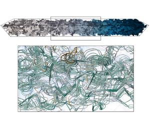The hydraulic aperture of each fracture is constant within each fracture and is the same for all fractures, $10^{-5}$ m. Isolated fractures and clusters of fractures are removed from the domain as they do not participate in the flow. The final network, illustrated in figure 1, contains 5660 fractures. The model medium is sufficiently large to quantify the impact of network heterogeneity in longitudinal large-scale transport. Due to computational limitations, the longitudinal extension of the domain is much larger than the transverse. Additional details of network generation are provided in the supplementary material available at https://doi.org/10.1017/jfm.2023.973.

Figure 1. Three-dimensional discrete fracture network composed of 5660 fractures. Fractures are coloured by pressure.

2.2. Fracture flow

2.2.1. Flow within a single fracture

We begin by considering flow through a single fracture. The laminar flow of an incompressible isothermal Newtonian fluid within a fracture is described by the Stokes equations

(2.1a,b)\begin{equation} \mu\,\nabla^2 {\boldsymbol{u}} - \boldsymbol{\nabla} P = 0, \quad \boldsymbol{\nabla} \boldsymbol{\cdot} {\boldsymbol{u}} = 0. \end{equation}

Here, ${\boldsymbol {u}}$ is the velocity vector, $\mu$ is the dynamic viscosity, and $\boldsymbol {\nabla } P$ is the fluid pressure gradient.

The fracture aperture is assumed to be constant and equal to $b$, which is small compared to the horizontal fracture extension. Moreover, we assume that the matrix surrounding the fractures is impervious, and there is no interaction between flow within the fractures and the solid matrix. Under these conditions, fracture flow is equivalent to flow through a Hele-Shaw cell, and the flow velocities can be approximated locally as quadratic functions of the vertical coordinates (Batchelor Reference Batchelor2000). Thus integration of the flow field across the aperture yields for the volumetric flow rate per unit length of fracture ${\boldsymbol {Q}}$ the Darcy-type equation

(2.2)\begin{equation} {\boldsymbol{Q}} ={-} T\,\boldsymbol{\nabla} P, \end{equation}

where $T = b^3/12 \mu$ is the fracture transmissivity, which is known as the cubic law. Thus we are representing the fractures as two-dimensional planes with resistance to flow proportional to the cube of the hydraulic aperture. Because flow is incompressible, volume is conserved such that $\boldsymbol {\nabla }\boldsymbol {\cdot } {\boldsymbol {Q}} = 0$. Volume conservation together with (2.2) gives the Reynolds equation

(2.3)\begin{equation} \boldsymbol{\nabla}\boldsymbol{\cdot} ( T\,\boldsymbol{\nabla} P ) = 0 \end{equation}

for the pressure distribution in the fracture. The assumptions concerning surface roughness, Reynolds number and fluid properties required to arrive at (2.3) are detailed in Zimmerman & Bodvarsson (Reference Zimmerman and Bodvarsson1996). The flux in each fracture is given by $\boldsymbol {q} = \boldsymbol {Q}/b$, which satisfies

(2.4)\begin{equation} {\boldsymbol{q}} ={-} \frac{k}{\mu}\,\boldsymbol{\nabla} P , \end{equation}

where the fracture permeability is defined by $k = b^2/12$.

2.2.2. Flow within a fracture network

Once fractures are placed into a network with other fractures, local boundary conditions modify the structure of the internal flow field within a single fracture, even in the case of a uniform hydraulic aperture. Specifically, the geometry of fractures, their boundaries and location of intersections within, along with network connectivity, leads to the formation of spatially variable velocity fields within a fracture plane even when flow is resolved using (2.3) on two-dimensional planar fractures. Neumann no-flow boundary conditions are imposed on the perimeter of all fractures and normal to the fracture plane; that is, there is no flow into the matrix. Within the network, pressure is a continuous and differentiable field that requires that pressure continuity along fracture intersections is imposed (Berre, Doster & Keilegavlen Reference Berre, Doster and Keilegavlen2019). Likewise, the flow volumetric rate needs to be divergence-free along intersections for an incompressible fluid. Note that the flux need not be continuous across the line of intersection. This discontinuity occurs if the values of apertures on the two intersecting fractures differ. The governing equations return values for the volumetric flow rate ${\boldsymbol {Q}}$, flux $\boldsymbol {q}$ and pressure $P$ throughout the network. To resolve transport, we need the spatially variable Eulerian velocity field ${\boldsymbol {u}} = \boldsymbol {q}/\phi$, where $\phi$ is the fracture porosity. Here, porosity is set to 1, that is, the fractures are fully open.

The probability density function (p.d.f.) of the Eulerian flow speed $v_e({\boldsymbol {x}}) = |{\boldsymbol {u}}({\boldsymbol {x}})|$ is a key quantity, as detailed below. It is defined through volumetric sampling as

(2.5)\begin{equation} p_e(v) = \frac{1}{V} \int_{\varOmega} {\rm d}\kern0.7pt {\boldsymbol{x}}\,\delta[v - v_e({\boldsymbol{x}})], \end{equation}

where $V$ is the volume of the flow domain $\varOmega$.

2.3. Particle motion

In this study, particle motion within the fracture network is due to advection only. We use a Lagrangian point of view and describe the transport of a solute particle starting at the point ${\boldsymbol {a}}$ by the kinematic equation

(2.6)\begin{equation} \frac{{\rm d}{\boldsymbol{x}}({t;{\boldsymbol{a}}})}{{\rm d} {t}} = {\boldsymbol{u}}[{\boldsymbol{x}}(t;{\boldsymbol{a}})]. \end{equation}

Molecular diffusion and mass exchange between fracture and matrix are not taken into account. It does impact the mean transport behaviour in the network. Furthermore, longitudinal dispersion is dominated by the network heterogeneity.

The distribution of a solute entering the fracture network is described typically using one of two conceptualizations, namely resident-based and flux-weighted injection (Kreft & Zuber Reference Kreft and Zuber1978). Physically, resident-based injection corresponds to a source that introduces a solute uniformly throughout an input area. For this reason, it is also referred to as uniform injection. In contrast, flux-weighted injection corresponds to a solute released in proportion to the inflowing volumetric flow rate at a location of insertion. These two injection modes are known to result in different transport behaviours through both fractured and heterogeneous porous media (Vanderborght, Mallants & Feyen Reference Vanderborght, Mallants and Feyen1998; Demmy, Berglund & Graham Reference Demmy, Berglund and Graham1999; Frampton & Cvetkovic Reference Frampton and Cvetkovic2009, Reference Frampton and Cvetkovic2011; Gotovac, Cvetkovic & Andricevic Reference Gotovac, Cvetkovic and Andricevic2009, Reference Gotovac, Cvetkovic and Andricevic2010; Janković & Fiori Reference Janković and Fiori2010; Hyman et al. Reference Hyman, Painter, Viswanathan, Makedonska and Karra2015; Kang et al. Reference Kang, Dentz, Le Borgne, Lee and Juanes2017, Reference Kang, Hyman, Han and Dentz2020; Comolli, Hakoun & Dentz Reference Comolli, Hakoun and Dentz2019; Puyguiraud, Gouze & Dentz Reference Puyguiraud, Gouze and Dentz2019). In this work, we study the transport behaviours emerging from both injection modes.

For the uniform injection, the initial particle positions are distributed uniformly across the fractures in the injection plane such that the initial particle density is $\rho ({\boldsymbol {a}}) = 1$. For the flux-weighted injection, the initial particle density is

(2.7)\begin{equation} \rho({\boldsymbol{a}}) = \frac{Q({\boldsymbol{a}})}{\langle Q \rangle}, \end{equation}

where $Q({\boldsymbol {a}}) = |\boldsymbol {Q}({\boldsymbol {a}})|$ is the magnitude of $\boldsymbol {Q}$, and $\langle Q \rangle$ is its average across the injection plane.

2.4. Observables

Macroscale transport through the fracture network is characterized by the distribution of particle arrival times, or breakthrough curves at different control planes within the network, as well as the longitudinal displacement mean and variance. The first passage or arrival time $\tau (x^\prime ;{\boldsymbol {a}})$ of a particle at a control plane located a linear distance $x^\prime$ in the primary direction of flow is defined by

(2.8)\begin{equation} \tau(x^\prime;{\boldsymbol{a}}) = \inf\{t\mid {{x}}(t;{\boldsymbol{a}}) \geq x^\prime\}. \end{equation}

Its distribution is given by

(2.9)\begin{equation} f(\tau,x^\prime) = \langle \rho({\boldsymbol{a}})\,\delta[\tau - \tau(x^\prime; {\boldsymbol{a}})] \rangle, \end{equation}

where the angular brackets denote the average over all particles. We refer to (2.9) as the first passage time distribution or breakthrough curve. The displacement mean and variance are defined by

(2.10a,b)\begin{equation} m_1(t) = \langle \rho({\boldsymbol{a}})\,{{x}}(t; {\boldsymbol{a}}) \rangle, \quad \sigma^2(t) = \langle \rho({\boldsymbol{a}})\,{{x}}(t;{\boldsymbol{a}})^2 \rangle - \mu(t)^2. \end{equation}

2.5. Numerical simulations

Once the network is generated, a conforming Delaunay triangulation of the network is created using the methods presented in Hyman et al. (Reference Hyman, Gable, Painter and Makedonska2014) and Krotz et al. (Reference Krotz, Sweeney, Gable, Hyman and Restrepo2022). An unstructured two-point flux finite-volume scheme is used to discretize the governing equations for flow (2.3). We apply Dirichlet boundary conditions for pressure to create a pressure difference $\Delta P =1$ MPa to drive flow from the $x = 0$ m face of the domain to the $x = 100$ m face. The particular value of the pressure difference is arbitrary because the governing equations are linear in $\boldsymbol {\nabla } P$. Therefore, the structure of the steady flow field, which is our primary interest, does not change with different pressure differences. Only its magnitude changes, which can be rescaled arbitrarily for our purposes. The model set-up creates a single principal flow direction, from which the flow within fractures can deviate. We use the massively parallel flow and reactive code pflotran (Lichtner et al. Reference Lichtner, Hammond, Lu, Karra, Bisht, Andre, Mills and Kumar2015) to integrate numerically the governing equations and obtain pressure and volumetric flow rates throughout the network, which are then used to reconstruct the Eulerian velocity field. Comprehensive details concerning the numerical simulations are provided in the supplementary material.

Figure 2 shows the Eulerian velocity distributions for the entire network and the inlet plane. The two distributions match well at the low-velocity end, but differ at high velocities. Thus the size of the injection plane is large enough to be representative of the global speed distribution at values smaller than the average speed. The undersampling of high speeds can be explained by the smaller probability to encounter speeds higher than the mean compared to speed smaller than the mean.

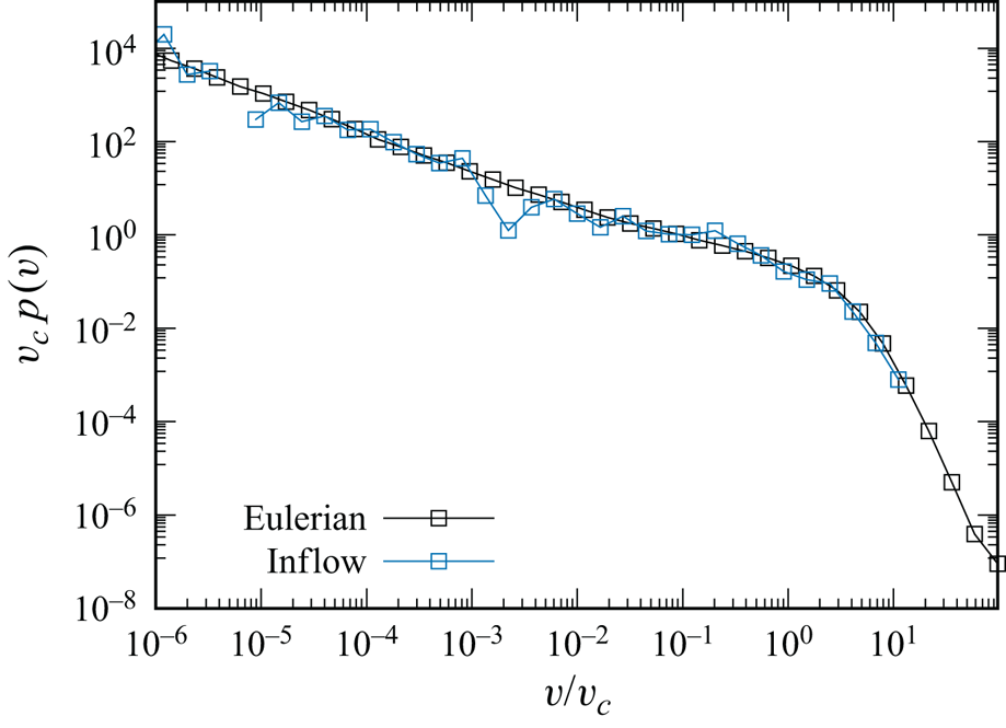
Figure 2. Eulerian velocity p.d.f.s for the entire network (black squares) and the inlet plane (blue squares). Speeds are rescaled by the Eulerian mean velocity $v_c$.

For the particle tracking simulations, we distinguish two sets of particles. In the first set, we follow $10^4$ particles and record all Lagrangian information. That is, spatial location, velocity and time are retained at every time step. In the second set, we follow $10^6$ particles and record their pathline length and travel time to reach uniformly spaced control planes placed at $\Delta x = 10$ m spacing through the domain. The use of different sets is a matter of computational limitations.

3.1. Kinematics

Rather than evolving on a characteristic time scale, particle motion in disordered media evolves on the length scales imprinted in the medium structure (Dentz et al. Reference Dentz, Kang, Comolli, Le Borgne and Lester2016). For random fracture networks, the evolution scales are imposed by the network geometry and its hydraulic properties. This is illustrated in figure 3, which shows the series of particle speeds as a function of time and as a function of distance along a trajectory. Plotted against time, the speed series shows an intermittent pattern with long periods of low speeds and islands of high speeds. Flow speeds are organized on a characteristic length scale, which is of the order of the mean fracture length $\ell _c$. Therefore, low velocities persist over much longer times than high velocities. In fact, plotted against distance, the speed series displays a regular random pattern that evolves on the scale of the mean fracture length $\ell _c$. Thus in order to gain insight into the structure and organization of flow and transport, we analyse the particle dynamics as a function of distance along trajectories.

Figure 3. Evolution of particle speeds with (a) time and (b) distance along a trajectory.

To this end, we note that the kinematic equation (2.6) can be formulated equivalently in terms of the distance ${s}(t;{\boldsymbol {a}})$ travelled by a particle along a streamline. The length ${s}(t;{\boldsymbol {a}})$ of the trajectory at a time $t$ is given by

(3.1)\begin{equation} \frac{{\rm d} {s}(t;{\boldsymbol{a}})}{{\rm d} t} = v_e[{\boldsymbol{x}}(t;{\boldsymbol{a}})]. \end{equation}

We use ${\rm d}s = v(s;{\boldsymbol {a}}) \,{\rm d}t$, where $v(s;{\boldsymbol {a}}) = v_e[{\boldsymbol {x}}(s;{\boldsymbol {a}})]$. For the kinematic equation (2.6), this gives

(3.2a,b)\begin{equation} \frac{{\rm d}\kern0.7pt {\boldsymbol{x}}({s};{\boldsymbol{a}})}{{\rm d} {s}} = \frac{{\boldsymbol{u}}[{\boldsymbol{x}}(s;{\boldsymbol{a}})]}{v({s;{\boldsymbol{a}}})}, \quad \frac{{\rm d} t({s};{\boldsymbol{a}})}{{\rm d} {s}} = \frac{1}{v({s};{\boldsymbol{a}})}. \end{equation}

We aim to quantify the stochastic dynamics of particle motion in the streamwise direction. We first focus on the motion along $s$, and specifically at the stochastic quantification of the series $\{v(s;{\boldsymbol {a}})\}$ of particle speeds.

3.2. Stochastic dynamics of particle speeds: Markov model and transition probabilities

In the following, we formulate the speed series $\{v(s;{\boldsymbol {a}})\}$ as a stationary Markov process and define its key statistics, the transition probability and the stationary speed distribution. We then analyse the structure of speed transitions using the copula densities that correspond to the empirical transition probabilities. Based on this analysis, we derive the resulting stochastic speed process that can be used to replace approaches based on empirical transition probabilities.

3.2.1. Speed statistics and Markov model

We represent the series $\{v(s;{\boldsymbol {a}})\}$ of particle speeds along a trajectory by the stochastic process $\{v(s)\}$, and replace the average over all particles by the ensemble average over all realizations of $v(s)$. Based on the random structure of the fracture networks under consideration, we pose $v(s)$ as a stationary Markov process continuous in $s$. This implies that the conditional probability $p(v,\Delta s|v')$ of two speeds separated by the lag distance $\Delta s$, the transition probability, obeys the Chapman–Kolmogorov equation (Risken Reference Risken1996)

(3.3)\begin{equation} p(v,s|v') = \int_0^\infty {\rm d}v''\,p(v,\Delta s|v'')\,p(v'',s - \Delta s|v'), \end{equation}

where $s \geq \Delta s$. The distribution $p(v,s)$ of particle speeds then evolves from any initial distribution $p_0(v)$ according to

(3.4)\begin{equation} p(v,s) = \int_0^\infty {\rm d}v' \,p(v,s|v')\,p_0(v'). \end{equation}

The steady-state distribution $p_s(v)$ is an eigenfunction of $p(v,s|v')$. In the following, we refer to $p(v,s|v')$ also as the transition probability from $v'$ to $v$. The Markov process is defined by two key quantities, the steady-state distribution $p_s(v)$ and the transition probability $p(v,s|v')$. Using Lagrangian ergodicity and the Reynolds theorem, it can be shown (Dentz et al. Reference Dentz, Kang, Comolli, Le Borgne and Lester2016) that $p_s(v,s)$ is given by the flux-weighted Eulerian speed distribution

(3.5)\begin{equation} p_s(v) = \frac{v\,p_e(v)}{v_c}, \end{equation}

where $v_c = \langle v_e \rangle$ is the mean Eulerian speed. Equation (3.5) relates a Eulerian quantity and a Lagrangian quantity, that is, a flow attribute and a transport attribute. It is a key step for the prediction of transport based on transport-independent quantities such as medium structure and Eulerian flow distribution.

Equations (3.3) and (3.4) describe a spatial Markov model for particle velocities, in the sense that $v(s)$ is a velocity that evolves in distance along a trajectory. Spatial Markov models for the evolution of particle velocities and transition times have been used in the literature for the modelling of non-Fickian transport features in porous and fractured media (Sherman et al. Reference Sherman, Engdahl, Porta and Bolster2021). The transition probabilities, which are at the head of these modelling approaches, are based typically on empirical transition matrices, which are obtained from particle tracking data. In the next subsubsection, we investigate the structure of spatial velocity transitions and their representation in terms of an analytical model.

3.2.2. Structure of speed process: copulas

The structure of the speed process $v(s)$, and thus the structure of hydrodynamic transport, is contained in the transition probability $p(v,s|v')$. In order to characterize $p(v,s|v')$, we focus on its copula density (Nelsen Reference Nelsen2013), which encodes the information on the correlation properties of $\{v(s)\}$ without bias from the marginal distribution. The copula density is equal to the transition probability of the unit score transforms $u(s)$ of $v(s)$, which are defined by

(3.6a,b)\begin{equation} u(s) = P_s[v(s)], \quad P_s(v) = \int_0^v {\rm d}v' \,p_s(v'), \end{equation}

where $P_s(v)$ is the cumulative distribution of $p_s(v)$. The transition probability from $u(s) = u'$ at $s$ to $u(s + \Delta s) = u$ at $s+\Delta s$ is given by

(3.7)\begin{equation} c(u,\Delta s|u') = \frac{p[P_s^{{-}1}(u),\Delta s|P_s^{{-}1}(u')]}{p_s[P_s^{{-}1}(u)]}. \end{equation}

Analogously, the speed transition probability can be written in terms of the copula density as

(3.8)\begin{equation} p(v,\Delta s|v') = c[P_s(v),\Delta s|P_s(v')]\,p_s(v). \end{equation}

Figure 4 shows the empirical copula density at different lag distances $\Delta s$, which are obtained from the trajectory data as outlined in Appendix A. The data can be represented by a stationary Gaussian copula, which is characterized by the exponential correlation function $\mathcal {C}(\Delta s) = \exp (-\Delta s /\ell _c)$ and the correlation length $\ell _c$; see Appendix B. The value $\ell _c = 2.2$ m fits the empirical data and is copacetic with the average fracture length.

Figure 4. Empirical copulas for lag distances $\Delta s = 0.5, 1, 2$ m. The solid lines denote iso-probability lines of the stationary Gaussian copula with correlation length $\ell _c = 2.2$.

As an immediate consequence of this finding, we note that the Gaussian copula provides an analytical model for the transition matrix in stochastic Markov models. The transition matrix can be constructed from the copula and the stationary speed distribution according to (3.8). In the following, we explore the implications of this observation further to identify the stochastic process for $v(s)$ and to derive the corresponding stochastic differential equation.

3.2.3. Stochastic speed process

First, we note that the fact that $\{v(s)\}$ can be described by a Gaussian copula implies that the normal score transform $w(s)$ of $v(s)$ is characterized by a multi-Gaussian distribution. The normal score transform is defined by

(3.9a,b)\begin{equation} w(s) = F^{{-}1}[v(s)] \equiv \varPhi^{{-}1}(p_s[v(s)]), \quad v(s) = F[w(s)] = p_s^{{-}1}(\varPhi[w(s)]), \end{equation}

where $\varPhi (w)$ is the cumulative unit normal distribution. The transition probability $p_w(w,{\rm d}s|w')$ from $w' = w(s)$ to $w = w(s + {\rm d}s)$ – that is, the distribution of $w(s + {\rm d}s)$ given that $w(s) = w'$ – is a Gaussian distribution with mean $w'\,\mathcal {C}({\rm d}s) \approx w' (1 - \ell _c^{-1} \,{\rm d}s)$ and variance $1 - \mathcal {C}(s)^2 \approx 2 \ell _c^{-1} \,{\rm d}s$. This implies that we can write $w(s + {\rm d}s)$ as

(3.10)\begin{equation} w(s + {\rm d}s) = w(s) \left(1 - \ell_c^{{-}1} \,{\rm d}s\right) + \sqrt{2 \ell_c^{{-}1} \,{\rm d}s}\, \zeta(s), \end{equation}

where $\zeta (s)$ is a Gaussian random variable of zero mean and unit variance. Taking the limit ${\rm d}s \to 0$ in (3.10), we obtain the following stochastic differential equation for $w(s)$:

(3.11)\begin{equation} \frac{{\rm d}w(s)}{{\rm d}s} = -\ell_c^{{-}1}\,w(s) + \sqrt{2 \ell_c^{{-}1}}\,\xi(s), \end{equation}

where $\xi (s)$ denotes a Gaussian white noise. Equation (3.11) describes an Ornstein– Uhlenbeck process, which has been used as a parsimonious model for speed series in pore-scale and Darcy-scale porous and fractured media (Morales et al. Reference Morales, Dentz, Willmann and Holzner2017; Hakoun, Comolli & Dentz Reference Hakoun, Comolli and Dentz2019; Hyman & Dentz Reference Hyman and Dentz2021). This indicates that the Gaussian copula structure may represent a general principle of organization of speed series in disordered media. In the following, we explore the consequences for $v(s)$ and $v(t)$ that follow from the representation of $w(s)$ as an Ornstein–Uhlenbeck process. Note that we use the same letter $v$ for spatial and temporally variable speed. We distinguish them through their argument.

By using the Ito lemma, we obtain for $v(s) = F[w(s)]$ from (3.11) the Langevin equation

(3.12)\begin{equation} \frac{{\rm d}v(s)}{{\rm d}s} ={-} \ell_c^{{-}1}\,A[v(s)] + \sqrt{2\,B[v(s)]\,\ell_c^{{-}1}}\,\xi(s), \end{equation}

where

(3.13)$$\begin{gather} A(v)= \left[- w\,\frac{{\rm d} F(w)}{{\rm d}w} + \frac{{\rm d}^2F(w)}{{\rm d}w^2} \right]_{w = F^{{-}1}(v)}, \end{gather}$$

(3.14)$$\begin{gather}B(v) = \left[\frac{{\rm d} F(w)}{{\rm d}w}\right]^2 _{w = F^{{-}1}(v)}. \end{gather}$$

The drift and diffusion coefficients $A(v)$ and $B(v)$ are fully defined by the Eulerian speed distribution $p_e(v)$. The initial particle velocities $v_0 = v(s = 0)$ are distributed according to $p_0(v)$, which depends on the injection condition. For uniform injection $p_0(v) = p_e(v)$, for flux-weighted injection, it is given by $p_0(v) = p_s(v)$. Thus (3.12) describes the evolution of the particle velocities for arbitrary injection conditions.

Equation (3.12) implies that the velocity distribution $p(v,s)$ evolves along a particle trajectory according to the Fokker–Planck equation

(3.15)\begin{equation} \frac{\partial p(v,s)}{\partial s} ={-} \frac{\partial}{\partial v} A(v)\,p(v,s) + \frac{\partial^2}{\partial v^2} B(v)\,p(v,s). \end{equation}

The stationary distribution $p_s(v)$ is given in terms of $A(v)$ and $B(v)$ as

(3.16)\begin{equation} p_s(v) = \frac{1}{B(v)} \exp\left[\int_{v_0}^v {\rm d}v'\,\frac{A(v')}{B(v')} \right]. \end{equation}

The integral limit $v_0$ is chosen such that the integral of the right-hand side is normalized to 1.

3.3. Stochastic particle motion

We focus on the streamwise particle motion, that is, along the direction of the mean flow velocity, which is aligned with the x-axis of the coordinate system. We project the displacement ${\rm d}s$ along the trajectory onto the streamwise displacement ${{\rm d}x}$ by using the advective tortuosity $\chi$, which compares the average trajectory length to linear distance. Thus we write

(3.17)\begin{equation} \frac{{{\rm d}x}(s)}{{\rm d}s} = \frac{1}{\chi}. \end{equation}

The evolution of the particle time $t(s)$ in this framework is given by

(3.18)\begin{equation} \frac{{\rm d} t(s)}{{\rm d}s} = \frac{1}{v(s)}, \end{equation}

where the velocity process $v(s)$ has been defined in the previous subsection. The advective tortuosity is given by (Koponen, Kataja & Timonen Reference Koponen, Kataja and Timonen1996)

(3.19)\begin{equation} \chi = \frac{\langle v_e \rangle}{u_{x}}, \end{equation}

that is, the ratio between the average velocity magnitude and the average velocity in the primary direction of flow.

Equations (3.12)–(3.18) describe a stochastic TDRW. Particle motion is determined as a function of distance $s$, and time $t(s)$ is a dependent variable. The presented framework allows us to derive the equations of motion for $[x(t),v(t)]$ through the variable change ${\rm d}s \to {\rm d}t$ in (3.17) and (3.12), which gives

(3.20)$$\begin{gather} \frac{{{\rm d}x}(t)}{{\rm d} t} = \frac{v(t)}{\chi}, \end{gather}$$

(3.21)$$\begin{gather}\frac{{\rm d}v(t)}{{\rm d}t} = v(t)\,A[v(t)] + \sqrt{2\,v(t)\,B[v(t)]}\,\xi(t). \end{gather}$$

The joint p.d.f. $p(x,v,t)$ then satisfies the Klein–Kramers equation (Risken Reference Risken1996)

(3.22)\begin{equation} \frac{\partial p(x,v,t)}{\partial t} + \frac{\partial}{\partial x} \left[\frac{v}{\chi}\, p(x,v,t)\right] ={-} \frac{\partial}{\partial v} v\,A(v)\,p(x,v,t) + \frac{\partial^2}{\partial v^2} v\, B(v)\,p(x,v,t). \end{equation}

This implies that the large-scale evolution of the joint p.d.f. of streamwise particle position and speed is fully defined by the Eulerian speed distribution, correlation length and tortuosity.

3.4. Continuous time random walk

As mentioned in the previous subsection, (3.17)–(3.18) represent a stochastic TDRW. For particle displacements $s \gg \ell _c$ much larger than the correlation length $\ell _c$, the velocity process $v(s)$ can be considered as uncorrelated. Using $\ell _c$ as the coarse graining scale, we define $s_n = n \ell _c$, $x(s_n) = x_n$ and $v(s_n) = v_n$. With these definitions, we can discretize (3.17) and (3.18) as

(3.23a,b)\begin{equation} x_{n+1} = x_n + \frac{\ell_c}{\chi}, \quad t_{n+1} = t_n + \frac{\ell_c}{v_n}. \end{equation}

The recursion relations (3.23a,b) describe a CTRW (Dentz et al. Reference Dentz, Cortis, Scher and Berkowitz2004; Berkowitz et al. Reference Berkowitz, Cortis, Dentz and Scher2006) for the turning point $x_n$, that is, the positions at which particles change speed. Unlike for other CTRW formulations (Berkowitz et al. Reference Berkowitz, Cortis, Dentz and Scher2006), here the distribution of transition times $\tau _n$ is in general not stationary because the distribution of $\tau _0$, the transition time for the first step, depends on the distribution of initial particle speeds, which varies according to the injection condition. This is an important feature, because large retention times in the injection region may have a strong impact on the overall plume evolution. In the following, we refer to the coarse-grained model (3.23a,b) as a CTRW, and the full model given by (3.17)–(3.18) as a stochastic TDRW.

The speed distributions $p_0(v)$ and $p_e(v)$ define the transition time distributions $\psi _0(t)$ for the first step and $\psi (t)$ for all following steps:

(3.24a,b)\begin{equation} \psi_0(t) = \frac{\ell_c}{t^2}\,p_0(\ell_c/t), \quad \psi(t) = \frac{\ell_c}{t^2}\,p_s(v) = \frac{\ell^{2}_c}{t^{3}v_c}\,p_e(\ell_c/t), \end{equation}

where we used the relation (3.5) between the steady-state speed distribution $p_s(v)$ and the Eulerian speed distribution $p_e(v)$. Unlike other CTRW formulations that assume a single transition time distribution that is fitted based on a suitable parametric function, (3.23a,b) provide a direct link to the underlying medium and Eulerian flow properties through the correlation length $\ell _c$ and the Eulerian speed distribution $p_e(v)$.

The particle distribution $p(x,t)$ satisfies

(3.25)\begin{equation} p(x,t) = \int_0^t {\rm d}t' \,R_0(x,t') \int_{t-t'}^{\infty} {\rm d}t''\, \psi_0(t'') + \int_0^t {\rm d}t'\,R(x,t') \int_{t-t'}^{\infty} {\rm d}t''\,\psi(t''), \end{equation}

where $R_0(x,t)$ is the distribution of initial particle position and time. Here, $R(x,t)$ denotes the frequency that a particle arrives at $x$ at time $t$. This equation reads as follows. The probability that a particle is at position $x$ at time $t$ is given by the probability that it remains at the initial position for a time larger than the current time (first term) plus the probability that it has just arrived at position $x$ and remains there for a time larger than $t$ (second term). Then $R(x,t)$ satisfies the equation

(3.26)\begin{equation} R(x,t) = \int_0^t {\rm d}t' \,\psi_0(t-t')\,R_0(x-\ell_c/\chi,t') + \int_0^t {\rm d}t'\, \psi(t-t')\,R(x-\ell_c/\chi,t'). \end{equation}

The first term on the right-hand side denotes the probability that the particle makes a transition from the initial position and time to $(x,t)$, while the second term denotes the probability that the particle makes a transition from any other possible position and time to $(x,t)$.

Combination of the Laplace transforms of (3.25) and (3.26) to eliminate $R^\ast (x,\lambda )$ gives for $p^\ast (x,\lambda )$ the equation

(3.27)\begin{align} \lambda p^\ast(x,\lambda) &= R_0(x,\lambda) - \frac{\psi^\ast(\lambda) - \psi_0^\ast(\lambda)}{1 - \psi^\ast(\lambda)}\left[R_0^\ast(x-\ell_c/\chi,\lambda) - R_0^\ast(x,\lambda) \right]\nonumber\\ &\quad + \frac{\lambda\,\psi^\ast(\lambda)}{1 - \psi^\ast(\lambda)} \left[p^\ast(x-\ell_c/\chi,\lambda) - p^\ast(x,\lambda)\right]. \end{align}

The Laplace transform is defined in Abramowitz & Stegun (Reference Abramowitz and Stegun1972). Laplace transformed quantities are marked by an asterisk, and the Laplace variable is denoted by $\lambda$. For $\psi _0(t) \equiv \psi (t)$, (3.27) is equal to the generalized master equation (Berkowitz et al. Reference Berkowitz, Cortis, Dentz and Scher2006). Note that (3.27) represents the coarse-grained projection of the Klein–Kramers equation (3.22) from $(x,v)$-space to $x$-space. The coarse-grained formulation of the stochastic TDRW as a CTRW allows us to obtain relatively compact Laplace-space expressions for the distribution of first passage times and the displacement moments, and facilitates the analytical prediction of their long-time scaling. The emphasis here is on the dependence of the long-time behaviour on the initial velocity distribution and thus the injection conditions, which have not been studied with other CTRW formulations.

3.4.1. First passage time distributions

The first passage times at linear distance $x_n$ are given by $t_{n}$, where $n = \inf (n|x_n \geq x)$, that is,

(3.28)\begin{equation} t_{n} = \sum_{j = 0}^{n-1} \frac{\ell_c}{v_j}. \end{equation}

The distribution $f_n(t)$ of first passage times is given by $f_n(t) = \langle \delta [t - t_n] \rangle$. It can be written in Laplace space as

(3.29)\begin{equation} f_n^\ast(\lambda) = \psi_0^\ast(\lambda)\,\psi^\ast(\lambda)^{n_c - 1} = \exp\left(\ln[\psi_0^\ast(\lambda)] + (n_c - 1) \ln[\psi^\ast(\lambda)] \right). \end{equation}

3.4.2. Displacement mean and variance

In order to determine the displacement mean and variance, we use the Fourier transform $\tilde {p}^\ast (k,\lambda )$ of $p^\ast (x,\lambda )$. It satisfies

(3.30)\begin{align} \lambda \tilde{p}^\ast(k,\lambda) &= 1 - \frac{\psi^\ast(\lambda) - \psi_0^\ast(\lambda)}{1 - \psi^\ast(\lambda)}\,[ \exp({\rm i} k \ell_c/\chi) - 1]\nonumber\\ &\quad + \frac{\lambda\,\psi^\ast(\lambda)}{1 - \psi^\ast(\lambda)}\,\tilde{p}^\ast(k,\lambda)\, [\exp({\rm i} k \ell_c/\chi) - 1], \end{align}

where we set $R_0^\ast (x,\lambda ) = \delta (x)$. The Fourier transform pair of a function $\varphi (x)$ is here defined by

(3.31a,b)\begin{equation} \tilde{\varphi}(k) = \int_{-\infty}^\infty {{\rm d}x} \exp({\rm i} k x)\,\varphi(x),\quad \varphi(x) = \int_{-\infty}^\infty \frac{{\rm d}k}{2 {\rm \pi}} \exp(-{\rm i} k x)\, \tilde{\varphi}(k), \end{equation}

with wavenumber denoted by $k$. We obtain from (3.30) for $\tilde {p}^\ast (k,\lambda )$ that

(3.32)\begin{equation} \tilde{p}^\ast(k,\lambda) = \frac{1}{\lambda}\,\frac{1 + \dfrac{\Delta \psi^\ast(\lambda)}{1 - \psi^\ast(\lambda)}\, \mathcal{F}(k)}{1 - \dfrac{ \psi^\ast(\lambda)}{1 - \psi^\ast(\lambda)}\,\mathcal{F}(k)}, \end{equation}

where we defined

(3.33a,b)\begin{equation} \mathcal{F}(k) = \exp({\rm i} k \ell_c/\chi) - 1, \quad\Delta \psi^\ast(\lambda) = \psi_0^\ast(\lambda) - \psi^\ast(\lambda). \end{equation}

The Laplace transform of the $n$th displacement moment is given in terms of $\tilde {p}^\ast (k,\lambda )$ as

(3.34)\begin{equation} m_n^\ast(\lambda) = (-{\rm i})^n \left.\frac{\partial \tilde{p}^\ast(k,\lambda)}{\partial k}\right|_{k = 0}. \end{equation}

The zeroth moment is 1 by definition because of the normalization of the particle distribution. The first and second moments are given by

(3.35)$$\begin{gather} m_1^\ast(\lambda) = \frac{1}{\lambda}\,\frac{\ell_c}{\chi}\, \frac{\psi_0^\ast(\lambda)}{1 - \psi^\ast(\lambda)}, \end{gather}$$

(3.36)$$\begin{gather}m_2^\ast(\lambda) = \frac{1}{\lambda}\,\frac{\ell_c^2}{\chi^2}\left[ \frac{\psi_0^\ast(\lambda)}{1 - \psi^\ast(\lambda)} +2\, \frac{\psi^\ast(\lambda)\,\psi_0^\ast(\lambda)}{[1 - \psi^\ast(\lambda)]^2} \right]. \end{gather}$$

The displacement variance is given by

(3.37)\begin{equation} \sigma^2(t) = m_2(t) - m_1(t)^2. \end{equation}

4.1. Speed statistics and transition times

Figure 5 shows the distribution $p_e(v)$ of Eulerian flow speeds and the Lagrangian speed distribution $p_s(v)$. The mean flow speed is $v_c = 357\ {\rm m}\ {\rm yr}^{-1}$. According to the theory, they are related by (3.5) through flux-weighting. This relation is confirmed by the numerical data presented in the figure. Furthermore, we observe that the behaviour of $p_e(v)$ at low flow speeds $v < 10^{-3} v_c$ can be approximated by the power law $p_e(v) \sim v^{\beta - 1}$ with $\beta = 0.1$. The high frequency of small flow speeds is remarkable given the relative regularity of the fracture network, which is characterized by constant fracture aperture, constant fracture length, but variable orientation; see § 2.1. Thus this broad distribution of flow speeds is due to the geometrical disorder of the fracture network. Current approaches to link flow speed and network characteristics are based on the Poiseuille law to link aperture distribution and speed. Such approaches do not apply here because the aperture is constant.

Figure 5. (a) Eulerian speed distribution $p_e(v)$, flux-weighted speed distribution and stationary Lagrangian speed distribution $p_s(v)$. The solid lines denote the scalings $v^{\beta -1}$ and $v^{\beta }$ with $\beta = 0.1$. (b) Corresponding transition time distributions. The solid lines denote the scalings $t^{-1-\beta }$ and $t^{-2-\beta }$.

The transition time distributions $\psi _0(t)$ and $\psi (t)$ corresponding to $p_e(v)$ and $p_s(v)$ are shown in figure 5(b). The characteristic transition time is $\tau _c = \ell _c / v_c$. The transition time distribution $\psi (t)$ scales as $t^{-2-\beta }$ for $t \gg \tau _c$. This implies for its Laplace transform $\psi ^\ast (\lambda )$ the behaviour

(4.1)\begin{equation} \psi^\ast(\lambda) = 1 - \lambda \tau_c + a (\lambda \tau_c)^{\beta+1}, \end{equation}

for $\lambda \tau _c \gg 1$, where $a$ is a constant, and the characteristic time $\tau _c$ is equal to the mean transition time. The transition time $\psi _0(t)$ for the initial step scales as $t^{-1-\beta }$ for $t \tau _c$. This implies for its Laplace transform that

(4.2)\begin{equation} \psi_0^\ast(\lambda) = 1 - a_0 (\lambda \tau_c)^{\beta}, \end{equation}

where $a_0$ is a constant.

4.2. First passage time distributions

Figure 6 shows the first passage time distribution ($\,fptd$) at different distances $x = 10$, $40$, $100$ and $1000$ m from the inlet plane. We observe tailing for both injection conditions. For the uniform injection, tailing is much stronger, i.e. slower decay, than for flux-weighted. Recall that the difference between the uniform and flux-weighted injection is the relative increase of particles in low-flow regions for uniform compared to flux-weighted injection. Thus stronger retention of particles at the inlet plane for uniform injection causes the broadening of the first passage time distribution towards long times. The stochastic TDRW model predicts accurately both the peak and tail behaviours for uniform and flux-weighted injection, and thus seems to capture the correct large-scale propagator of the complex flow and transport system. The late-time behaviour for the uniform injection is characterized by the power-law scaling $t^{-1-\beta }$. For the flux-weighted injection, the tails scale as $t^{-2-\beta }$. This latter scaling is a consequence of the generalized central limit theorem. In fact, the arrival time distribution converges towards a stable distribution with distance from the inlet (Hyman et al. Reference Hyman, Dentz, Hagberg and Kang2019a).

Figure 6. Arrival time distributions at distances (top left to bottom right) $x = 10, 40, 100, 1000$ m from the inlet. Symbols correspond to the numerical simulations, and solid lines to the stochastic TDRW model for (orange) flux-weighted and (black) uniform injection. The dash-dotted lines indicate the scaling $t^{-1-\beta }$, and the dashed lines indicate the scaling $t^{-2-\beta }$, with $\beta = 0.1$.

For the convenience of the reader, we summarize the main arguments in the following. We start from (2.9) for the Laplace transform of the arrival time distribution in the equivalent CTRW. For the flux-weighted injection, we can write for $\lambda \tau _c \gg 1$ that

(4.3)\begin{equation} f^\ast_n(\lambda) = \exp\left(- \langle t_n \rangle \lambda\right) g_n^\ast[\lambda \langle t_n \rangle^{1/(1+\beta)}], \end{equation}

where we defined

(4.4)\begin{equation} g_n^\ast(\lambda) = \exp\left[\frac{a}{\tau_c}\,(\lambda \tau_c)^{1 + \beta} + \cdots\right]. \end{equation}

Note that $\langle t_n \rangle = n \tau _c$. To arrive at (4.3), we used (4.1) for the Laplace transform $\psi ^\ast (\lambda )$ of $\psi (t)$, and Taylor expanded the logarithm in (2.9). The dots in (4.4) denote contributions that go to zero in the limit $n \to \infty$ (Hyman et al. Reference Hyman, Dentz, Hagberg and Kang2019a). Thus $\lim _{n\to \infty } g_n(\lambda ) = g_\beta ^\ast (\lambda )$, where $g_\beta ^\ast (\lambda ) = \exp [a (\lambda \tau _c)/\tau _c]$ is a stable density that is totally skewed to the right. This implies that for large $n$, $f_n(t)$ tends towards the scaling form:

(4.5)\begin{equation} f_n(t) \to \frac{g_\beta[(t - \langle t_n \rangle)/\langle t_n \rangle^{1/(1+\beta)}]}{\langle t_n \rangle^{1/(1+\beta)}}. \end{equation}

Figure 7 illustrates the tail behaviours for flux-weighted injection at different distances. They collapse on the same curve when rescaled appropriately, according to their stable limit.

Figure 7. Arrival time distributions for (a) flux-weighted and (b) uniform injection at distances $x = 10, 40, 100, 1000$ m from the inlet from (symbols) numerical simulations and (solid lines) the stochastic TDRW model. The black solid line denotes the prediction of the stochastic TDRW model for $x = 1000\ {\rm m}$. (b,d) The same data as in corresponding panels (a,c) rescaled according to (4.3). The red lines denote the scaling form given by (4.5). Note that we display only the data from the stochastic TDRW model, which are sufficient due to the agreement with the data from the numerical simulations shown in (a,c).

This is different for the uniform injection. We see from figure 6 that the peak behaviours of the flux-weighted and uniform injections converge with increasing distance from the inlet. The tail behaviour, however, is distinctly different, characterized by different exponents. Moreover, the tails collapse on the same curve. This is emphasized in figure 7, in which the arrival time distributions for uniform injection are rescaled according to (4.5). The peak behaviours are similar to those for the flux-weighted injection, and seem to converge to the stable form. The tails of the rescaled arrival time distributions do not collapse onto a single curve. Thus there seems to be convergence in the bulk, but not in the tails of the distribution. This behaviour can be explained by inspecting again (2.9), which now can be written as

(4.6)\begin{equation} f^\ast_n(\lambda) = \psi_0^\ast(\lambda) \exp\left(- \langle t_{n-1} \rangle \lambda\right) g_{n-1}[\lambda \langle t_{n-1} \rangle^{1/(1+\beta)}], \end{equation}

where $\langle t_{n-1} \rangle = (n-1) \tau _c$. Thus, in the limit of $n \gg 1$, the arrival time distribution can be written as

(4.7)\begin{equation} f_n(t) = \int_0^t {\rm d}t'\,\psi_0(t - t')\,\frac{g_\beta[(t' - \langle t_n \rangle)/\langle t_n \rangle^{1/(1+\beta)}]}{\langle t_n \rangle^{1/(1+\beta)}}. \end{equation}

It is the convolution of the initial transition time distribution with the stable distribution. The long-time tail is due to the first time step, which all arrival time distributions have in common. Therefore, the tails collapse on the same curve. The peak behaviour, on the other hand, stems from the summation of transition times that are distributed according to $\psi (t)$. This explains the convergence of the peak behaviour to the peak of the stable law. In summary, the bulk of the arrival time distribution converges to a stable law, and the tail retains the memory of the velocity at the injection plane.

4.3. Displacement mean and variance

Figure 8 shows the displacement mean and variance for uniform and flux-weighted injections. The observation times are smaller than the time when the first particles leave the domain. Due to the occurrence of fast pathways, this time is relatively short. The upscaled theory reproduces the evolution of the displacement mean for both injection conditions.

Figure 8. Displacement (a) mean and (b) variance from (symbols) numerical simulations and (solid lines) the stochastic TDRW model for (orange) flux-weighted and (black) uniform injection. The dashed lines show the long-time predictions of the CTRW model described in § 3.4. The dotted line indicates the power-law behaviour (4.11).

The early-time behaviour of the mean displacement is given by

(4.8)\begin{equation} m_1(t) = \langle v_0 \rangle t/\chi, \end{equation}

where $\langle v_0 \rangle$ is the mean initial speed. Its asymptotic long-time behaviour is

(4.9)\begin{equation} m_1(t) = v_c t/\chi, \end{equation}

because the temporal speed statistics asymptote towards $p_e(v)$. The displacement variance at early times shows ballistic behaviour, which is due to the persistence of the initial velocities,

(4.10)\begin{equation} \sigma^2(t) = \frac{\sigma_{v_0}^2}{\chi^2}\,t^2, \end{equation}

where $\sigma _{v_0}^2$ is the variance of the initial speed distribution $p_0(v)$. After the ballistic early-time regime, the variances cross over to a power-law regime that is determined by the exponent $\beta$ that determines the behaviour of $p_e(v)$ at $v \ll v_c$; see figure 5. From the explicit Laplace space expressions (3.35) and (3.36), we can derive the following asymptotic expressions for the uniform and flux-weighted initial conditions:

(4.11)$$\begin{gather} \sigma^2(t) = \frac{v_c^2}{\chi^2}\,t^{2-\alpha}\,\frac{2 \alpha a + 2 a_0 (1 - \alpha)}{\varGamma(3 - \alpha)}, \end{gather}$$

(4.12)$$\begin{gather}\sigma^2(t) = \frac{v_c^2}{\chi^2}\,t^{2-\alpha}\,\frac{2 \alpha a}{\varGamma(3 - \alpha)}, \end{gather}$$

respectively. We used expressions (4.1) and (4.2).

For the uniform injection, the temporal velocity statistics are stationary; see § 3.2. Therefore, as shown in figure 8, the mean transport speed is equal to the Eulerian mean speed $v_c = \langle v_e \rangle$, and the displacement mean evolves linearly with time according to (4.9). The numerical early-time data are slightly below the model prediction. This is due to the fact that the initial speed distribution $p_0(v)$ deviates from $p_e(v)$ at high speeds, as shown in figure 2, which implies that the initial mean speed is smaller than $\langle v_e \rangle$. A similar behaviour is observed for the flux-weighted injection, for which the theory predicts the early-time behaviour $m_1(t) = v_f t /\chi$, where $v_f$ denotes the mean of $p_s(v)$. It is given by $v_f = {\langle v_e^2 \rangle }/{\langle v_e \rangle }$, where $\langle v_e^2 \rangle$ is the mean squared Eulerian flow speed. Here as well, the numerical data are slightly below the model prediction. For both injection modes, the mean displacements converge for times $t \gg \tau _c$ because the temporal velocity statistics asymptote towards $p_e(v)$.

As outlined above, the early-time behaviour of the displacement variance is ballistic, characterized by the initial speed variance. Also here, the model prediction slightly overestimates the numerical data; see figure 8. The variance for the flux-weighted injection is initially larger than for the uniform injection because of the higher initial speed variance. Then for times larger than the mean advection time $\tau _c$, it slows down and remains at smaller values than for the uniform injection. The long-time evolution for both injection conditions is characterized by the power-law behaviour predicted in (4.11). At times $t \gg \tau _c$, the variance for the uniform injection grows faster than for the flux-weighted injection because there is a a stronger temporal persistence of lower velocities. The persisting contrast between slow particles and fast particles leads to faster growth.

The theoretical model captures the early-time behaviour of tracer displacement and dispersion, and predicts anomalous dispersion at large times caused by the broad distribution of flow speeds. The asymptotic dispersion behavior and the difference between injection conditions is also captured by the proposed CTRW model that accounts for arbitrary initial transition time distributions.