3.1. Drag and lift forces

Figure 2 shows the numerical results for the drag and lift coefficients at ${{Re}}=0.2$. Clearly, both coefficients increase monotonically with increasing $\mu ^\ast$. This is consistent with the low-${{Re}}$ vortical mechanism (Legendre & Magnaudet Reference Legendre and Magnaudet1997; Magnaudet et al. Reference Magnaudet, Takagi and Legendre2003), which suggests that the drag and lift increase with increasing surface vorticity (i.e. the vorticity generated on the external side of the droplet) and, hence, with increasing viscosity ratio $\mu ^\ast$. Specifically, the vortical mechanism indicates that, to leading order, the drag (respectively, lift) force in the solid-sphere limit at low-but-finite ${{Re}}$ differs from that in the clean-bubble limit only by a prefactor of $3/2$ (respectively, $(3/2)^2$), $3/2$ being the ratio of the maximum surface vorticity, $\omega _s$, in these two limits. This is confirmed by our numerical results, noting that $C_D$ (respectively, $C_L$) at $\mu ^\ast =100$ is larger than that at $\mu ^\ast =0.01$ by a factor of 1.54 (respectively, 2.15).

Figure 2.

Results for $C_D$ and $C_L$ as a function of $\mu ^\ast$ for ${{Re}}=0.2$, ${{Re}}^\ast =5$ and $Sr=0.2$. Red circles, present numerical results. In panel (a), $C_D$ is multiplied by ${{Re}}$ for better readability; fitted line, (3.3a) with $m=1$. In panel (b), fitted line, (3.3b); solid line, $C_L^{S(2)}$ according to (B3); dotted line, $C_L^{B(1)}$ according to (B4b).

Figure 3 presents the results for $C_D$ and $C_L$ within the low-to-moderate Reynolds number regime, $0.5 \leq {{Re}} \leq 20$. At a given ${{Re}}$, the computed $C_D$ gradually increases with increasing $\mu ^\ast$, still aligning with the low-${{Re}}$ vortical mechanism. However, the behaviour of $C_L$ differs. Specifically, $C_L$ increases gradually with increasing $\mu ^\ast$ only up to ${{Re}} \approx 2$. For ${{Re}} \geq 5$, it decreases as $\mu ^\ast$ increases. This latter behaviour is not surprising. As ${{Re}}$ increases, the ratio of the Oseen and Saffman lengths, $\varepsilon = (Sr/{{Re}} )^{1/2}$, a key parameter characterizing the magnitude of inertial lift (McLaughlin Reference McLaughlin1991), decreases as well. For ${{Re}} \gtrsim 5$, the lift generation is governed by the competition between the ‘$L$’ and ‘$S$’ mechanisms outlined in § 1. This competition will be elaborated on in more detail in § 3.3. Here, we briefly mention that the decrease in $C_L$ with increasing $\mu ^\ast$ for ${{Re}} \geq 5$ is closely related to the increase in the maximum surface vorticity $\omega _s$. This increase enhances the ‘$S$’ mechanism, resulting in an increasingly negative lift contribution (i.e. towards $-\boldsymbol {e}_y$) (Adoua et al. Reference Adoua, Legendre and Magnaudet2009; Hidman et al. Reference Hidman, Ström, Sasic and Sardina2022).

Figure 3.

Similar to figure 2, but for $0.5 \leq {{Re}} \leq 20$, ${{Re}}^\ast = 5$ and $Sr = 0.2$. Different ${{Re}}$ values are distinguished using the colours indicated in panel (a). Different types of symbols are used to represent data for ${{Re}} > 5$, providing a clearer distinction for the $C_L$ results. In panel (a), solid lines correspond to predictions using (3.3a) with the expression for $m$ from (3.4). In panel (b), solid lines denote predictions from (3.3b) and the horizontal thin dashed line represents $C_L = 0$.

Figure 4 shows the drag and lift results at ${{Re}} = O(100)$. In contrast to the low-to-moderate ${{Re}}$ regime, where $C_D$ and $C_L$ vary monotonically with increasing $\mu ^\ast$, these coefficients exhibit non-monotonic behaviour at low-but-finite $\mu ^\ast$. For instance, $C_D$ at ${{Re}} = 250$ reaches a local maximum of 0.65 at $\mu ^\ast = 2$, corresponding to 91 % of that for a solid sphere, and then gradually decreases as $\mu ^\ast$ increases from 2 to 5. At the same ${{Re}}$, $C_L$ attains a local maximum of 0.24 at $\mu ^\ast \approx 0.5$, approximately 1.8 times larger than that predicted by the inviscid solution (Auton Reference Auton1987), namely $C_L=2Sr/3$. This latter behaviour is particularly surprising since, as discussed in § 1 and shown in figure 3(b), the competition between the ‘$L$’ and ‘$S$’ mechanisms in generating the lift at ${{Re}} = O(100)$ would suggest that: (i) an increase in $\mu ^\ast$ should result in a monotonic decrease in $C_L$ and (ii) the maximum $C_L$ should correspond to the inviscid solution and be achieved at the smallest $\mu ^\ast$. Moreover, to the best of our knowledge, no such non-monotonic behaviour in the lift force has been reported until now.

Figure 4.

Similar to figure 2, but for $50\leq {{Re}}\leq 250$, ${{Re}}^\ast =5$ and $Sr=0.2$. Different colours denote different ${{Re}}$ as indicated in panel (a). Symbols crossed by dashed lines represent numerical results. In panel (a), solid lines denote $C_D$ predictions using (3.3a) with $m$ given by (3.4). In panel (b), solid lines denote $C_L$ predictions using (3.5)–(3.9a–e), horizontal dashed line denotes the lift solution in the inviscid limit (Auton Reference Auton1987), namely $C_L = 2Sr/3$.

In figure 4, the non-monotonic evolution of $C_D$ and $C_L$ sets in beyond ${{Re}}\approx 100$. However, it is not immediately clear whether this Reynolds number dependency is driven by the inertia of the external fluid (i.e. ${{Re}}$) or the internal fluid (i.e. ${{Re}}^i$). So far, the Reynolds number ratio has been fixed at ${{Re}}^\ast ={{Re}}^i/{{Re}}=5$, where ${{Re}}^i$ is based on the kinematic viscosity of the internal fluid, meaning both Reynolds numbers were varied simultaneously. To clarify the dependency on the internal fluid inertia, additional simulations were conducted at a fixed external Reynolds number of ${{Re}}=200$, varying ${{Re}}^\ast$ from 0.2 to 10. This covers a range for ${{Re}}^i$ from 40 to 2000. Given the relation $\rho ^\ast ={{Re}}^\ast \mu ^\ast$, these additional runs also cover a wide range of density ratios, for $\rho ^\ast$ from $10^{-2}$ to $10^{3}$. The corresponding results for $C_D$ and $C_L$ are summarized in figure 5. These results distinctly demonstrate that it is the inertia of the internal fluid that drives the non-monotonic variation of both $C_D(\mu ^\ast )$ and $C_L(\mu ^\ast )$. Notably, for ${{Re}}^i$ smaller than approximately 300 (i.e. ${{Re}}^\ast \lesssim 1.5$), both $C_D$ and $C_L$ depend solely on $\mu ^\ast$, consistent with findings in the low-${{Re}}$ limit (Magnaudet et al. Reference Magnaudet, Takagi and Legendre2003). Intriguingly, the computed $C_D$ under this condition aligns well with numerical data at $Sr=0$ from Feng & Michaelides (Reference Feng and Michaelides2001), which were obtained by imposing the flow to be axisymmetric regardless of $\mu ^\ast$. Conversely, for ${{Re}}^i>300$ (i.e. ${{Re}}^\ast >1.5$) and $\mu ^\ast$ below a critical value $\mu _c^\ast$ that increases with ${{Re}}^i$, the computed $C_D$ and $C_L$ are typically larger than their counterparts in cases where ${{Re}}^i\lesssim 300$. The sole exception occurs at $({{Re}}^i,\mu ^\ast )=(2000,5)$, where $C_L$ is smaller than those at lower ${{Re}}^i$ values. These distinct behaviours for $\mu ^\ast < \mu _c^\ast$ are found to be closely linked to the internal 3-D flow bifurcation, a scenario that will be detailed in § 3.2.

Figure 5.

Results for $C_D$ and $C_L$ as a function of $\mu ^\ast$ for $0.2\leq {{Re}}^\ast \leq 10$, ${{Re}}=200$ and $Sr=0.2$. Different values of ${{Re}}^\ast$ are denoted by different colours as indicated in panel (a). The internal Reynolds number is ${{Re}}^i={{Re}}{{Re}}^\ast$. In panel (a), fitted line, $C_D$ prediction using (3.3a) and (3.4); black triangle, data at $Sr=0$ from Feng & Michaelides (Reference Feng and Michaelides2001) obtained by imposing the flow to be axisymmetric. In panel (b), fitted line, $C_L$ prediction using (3.5)–(3.9a–e).

3.2. Identification of the internal 3-D flow bifurcation

The non-monotonic evolution of $C_D(\mu ^\ast )$ outlined in the preceding section is not exclusive to shear flows. To corroborate this, we conducted additional simulations for droplets with varying viscosity ratios in a uniform flow (i.e. with $Sr=0$). Figure 6 compares the time histories of $C_D$ obtained at $Sr=0$ (red dashed line) and $Sr=0.2$ (red solid line); for both cases, $({{Re}}, {{Re}}^\ast, \mu ^\ast ) = (200, 5, 0.5)$. By introducing a time shift $t_0=166R/u_{rel}$ and setting $t^\ast =(t-t_0)u_{rel}/R$ (respectively, $t^\ast =tu_{rel}/R$) for $Sr=0$ (respectively, 0.2), the two evolutions almost coincide beyond $t^\ast \approx 30$. Before this, both cases reach a quasi-steady value of $C_D \approx 0.32$, close to the value reported by Feng & Michaelides (Reference Feng and Michaelides2001) for an axisymmetric flow. These observations suggest a flow bifurcation sets in prior to $t^\ast \approx 30$, after which the flow becomes strongly non-axisymmetric. This non-axisymmetric flow structure can be visualized using the streamwise vorticity, $\omega _x$, as illustrated in figure 7.

Figure 6.

Time history of $C_D$ (in red) and $C_L$ (in green) for $({{Re}}, {{Re}}^\ast, \mu ^\ast ) = (200, 5, 0.5)$. Dashed lines, $Sr=0$; solid lines, $Sr=0.2$. For $Sr=0$, a time shift $t_0=166R/u_{rel}$ is applied and evolutions are plotted versus the normalized, modified time $t^\ast =(t-t_0)u_{rel}/R$. For $Sr=0.2$, no such time shift is applied and $t^\ast =tu_{rel}/R$. For the case $Sr=0$, since no flow perturbation was imposed to trigger the bifurcation, $C_L$ is calculated as $C_L=\sqrt {C_y^2+C_z^2}$, where $C_y$ and $C_z$ are the coefficients of the hydrodynamic force components along $y$ and $z$, respectively.

Figure 7.

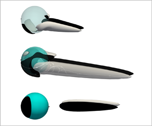
Isosurfaces of the streamwise vorticity $(R/u_{rel})\boldsymbol {\omega } \boldsymbol {\cdot } \boldsymbol {e}_x = \pm 0.5$ in the wake of the droplet for $({{Re}}, {{Re}}^\ast, \mu ^\ast ) = (200, 5, 0.5)$ at five selected time points. Panels (i) correspond to $Sr=0$ and panels (ii) to $Sr=0.2$. In all panels, negative values are denoted by black threads, while the droplet surface is represented as a partially transparent, light blue-coloured sphere.

When the ambient flow is uniform ($Sr=0$), the flow remains axisymmetric prior to the bifurcation (up to $t^\ast \approx 20$), as indicated by the absence of $\omega _x$ structure in figure 7(a-i) (corresponding to $t^\ast = 20$). The flow bifurcation sets in at $t^\ast \approx 25$, first manifesting as non-axisymmetric flow inside the droplet (figure 7b-i), while the external flow retains its axisymmetry. This disturbance grows in time, eventually extending outside the droplet by $t^\ast \approx 30$ (figure 7c-i), peaking in intensity at $t^\ast \approx 37.5$ (figure 7d-i), and then slightly decaying and stabilizing after $t^\ast \approx 120$ (figure 7e-i). Correlating this with the time evolution of $C_D$ in figure 6, a direct link is evident between the drag increase (compared with the drag in the axisymmetric case) and the vortical intensity in the wake. This correlation can be attributed to the ‘sucking’ effect by the droplet's 3-D wake, where the low-pressure cores of vortical threads increase the pressure difference between the front and back regions of the droplet. Thus, a stronger $\omega _x$ in the wake is related to a larger drag increase. Moreover, as the streamwise vorticity structure remains bi-planar symmetric, no lift force is expected on the droplet throughout the process, as confirmed by figure 6 (dashed green line).

In the presence of shear ($Sr=0.2$), the flow exhibits slight non-axisymmetry prior to the onset of the corresponding imperfect bifurcation. This is evident from the vortical structure at $t^\ast =20$ (figure 7a-ii), where two streamwise vorticity threads are visible inside and extending outside the droplet in the near wake. Owing to the ‘sucking’ effect, the drag is slightly higher than in the $Sr=0$ case. Additionally, the orientation of these vortical threads results in a small but measurable lift force (Auton Reference Auton1987; Legendre & Magnaudet Reference Legendre and Magnaudet1998), as shown in figure 6 (solid green line). Moreover, $C_L=Sr$ at $t=0^+$ according to figure 6, consistent with the analytical solution derived by Legendre & Magnaudet (Reference Legendre and Magnaudet1998). As the bifurcation sets in, similar to the $Sr=0$ case, it is initially the internal flow that shows pronounced non-axisymmetry (figure 7b-ii). This non-axisymmetry intensifies over time, extending outside the droplet by $t^\ast \approx 30$ (figure 7c-ii), and peaks at $t^\ast \approx 37.5$ (figure 7d-ii). Interestingly, the $\omega _x$ structure at $t^\ast \approx 37.5$ resembles the bi-planar symmetry seen in the $Sr=0$ case, which is why the lift at this time moment is even smaller than that before the onset of bifurcation. However, as time progresses, the $\omega _x$ threads in the half-space $y>0$ shrink rapidly, and the reverse is the case for the other two threads, leading the flow to revert to its initial structure with only two significant $\omega _x$ threads in the final stage (compare figure 7e-ii with figure 7a-ii). Since the intensity of the two vortical threads in the final stage is significantly larger that that before the onset of bifurcation, the lift force is highly increased.

Similar flow characteristics are observed in cases at different ${{Re}}^\ast$. Figure 8 summarizes the final-state results for $C_D$ and $C_L$ at different ${{Re}}^\ast$, all obtained at $({{Re}}, \mu ^\ast )=(200, 0.5)$. These results confirm a critical Reynolds number for flow bifurcation at ${{Re}}_c^i\approx 300$ (i.e. ${{Re}}^\ast =1.5$ at ${{Re}}=200$), aligning with findings in figure 5. From these final-state results, and the time evolution of the hydrodynamic forces and flow structures (figures 6 and 7), we conclude that irrespective of the presence of shear, the flow can undergo bifurcation leading to strong non-axisymmetry, marked by multiple threads of streamwise vorticity in the droplet wake. The flow bifurcation identified here differs from that in prior work on a uniform flow past a solid sphere or an oblate spheroidal bubble (Johnson & Patel Reference Johnson and Patel1999; Magnaudet & Mougin Reference Magnaudet and Mougin2007; Fabre et al. Reference Fabre, Tchoufag and Magnaudet2012; Citro et al. Reference Citro, Tchoufag, Fabre, Giannetti and Luchini2016), where the internal flow is irrelevant, and bifurcation occurs when the maximum vorticity on the external side of the body surface exceeds a critical, ${{Re}}$-dependent value, say $\omega _{c}^e({{Re}})$. Here, internal flow is crucial, as non-axisymmetry initially manifests only within the droplet. Conversely, the external vorticity at the droplet surface, which increase with the viscosity ratio, is not relevant, as the bifurcation only happens for $\mu ^\ast < \mu _c^\ast$, a regime where the external surface vorticity remains lower than the corresponding $\omega _{c}^e$. Given these distinct features, we term the phenomenon in our work internal bifurcation, distinguishing it from the external one observed with solid spheres or non-spherical bubbles. The underlying mechanism of this internal bifurcation warrants a further systematic investigation under uniform-flow conditions, which is beyond the scope of the present work. Nevertheless, some preliminary ideas will be provided in § 4.

Figure 8.

Results for $C_D$ and $C_L$ as a function of ${{Re}}^\ast$ for $Sr=0$ ($+$, red) and 0.2 ($\bigcirc$, red) under the condition ${{Re}}=200$ and $\mu ^\ast =0.5$. The shaded grey region corresponds to the regime where the flow past the droplet remains axisymmetric for $Sr=0$.

Before moving to the next section, it is important to highlight another key change in the flow structure before and after the onset of internal bifurcation, due to its close relation to lift generation. To begin, we illustrate in figure 9(a-i–a-iii) the streamlines for the case $(Sr, {{Re}}, {{Re}}^\ast, \mu ^\ast ) = (0, 200, 5, 0.5)$ at $t^\ast =120$. Four threads of swirling flow can be identified both inside and outside the drop, particularly in the region close to the back surface of the drop. It then becomes clear that the counter-rotating streamwise vortices in the wake originate largely from the swirling flow generated inside the drop during the transition from axisymmetric to biplanar symmetric flow. As the swirling flow propagates downstream in the wake, the radial pressure gradient associated with the swirling motion tends to confine the flow, driving the fluid particles towards the centre of each vortical thread. Mass conservation indicates that the flow must accelerate along the streamwise direction, leading to an increase in the extensional rate (i.e. $\partial u_x / \partial x$) in the wake. To highlight this confinement induced by the swirling flow, we compare the streamtubes before ($t^\ast =20$) and after ($t^\ast =120$) the onset of flow bifurcation. Specifically, we consider the streamtube formed by all streamlines passing through the circle $[x=-2R, (y^2+z^2)=(0.25R)^2]$. Before the onset of flow bifurcation (figure 9b-i–b-ii), the cross-stream section of the streamtube remains circular downstream and experiences only moderate confinement for $x\gtrsim 1.5R$. In contrast, after the onset of flow bifurcation (figure 9c-i–c-ii), the streamtube is highly squeezed, such that the cross-sectional area in the wake is concentrated into the four vortical threads. Specifically, from $x=2R$ to $x=3R$, the cross-sectional area decreases from $0.316R^2$ to $0.182R^2$, a relative decrease of approximately 42 %, whereas the relative decrease is only approximately 24 % in the case without the onset of flow bifurcation. This pronounced confinement is closely linked to the amplification of the streamwise vorticity and, hence, to lift generation. The details of this will be discussed in § 3.3.

Figure 9.

Streamlines and streamtubes for the case $(Sr, {{Re}}, {{Re}}^\ast, \mu ^\ast ) = (0, 200, 5, 0.5)$. (a-i–a-iii) Streamlines inside (red) and outside (black) the drop, and close to the back surface of the drop at $t^\ast =120$. The coordinates $y$ and $z$ denote the extension and compression directions of the straining flow in the wake, respectively. (b-i,c-i) Streamtubes formed by all streamlines (coloured in magenta) passing through the circle $[x=-2R, (y^2+z^2)=(0.25R)^2]$ at $t^\ast =20$ and $t^\ast =120$, respectively. (b-ii,c-ii) Corresponding profiles of the streamtube at different distances downstream: red line, $x=R$ green line, $x=1.5R$; blue line, $x=2R$; and cyan line, $x=3R$.

3.3. Mechanism of the lift generation at ${{Re}}=O(100)$

3.3.1. Relation between lift force and streamwise vorticity

The lift force on a three-dimensional body moving at ${{Re}}=O(100)$ is closely related to the presence of a pair of streamwise vortices in its wake (Auton Reference Auton1987; Legendre & Magnaudet Reference Legendre and Magnaudet1998; Adoua et al. Reference Adoua, Legendre and Magnaudet2009; Shi et al. Reference Shi, Rzehak, Lucas and Magnaudet2021; Hidman et al. Reference Hidman, Ström, Sasic and Sardina2022). Specifically, the direction of the lift force is determined by the orientations of these vortices. Figure 10(a-i–a-vi) illustrates the isosurfaces of the streamwise vorticity at various $\mu ^\ast$ for ${{Re}}=200$, ${{Re}}^\ast =5$ and $Sr=0.2$. The intensity of the streamwise vortices increases as $\mu ^\ast$ increases from 0.01, reaching a local maximum at $\mu ^\ast \approx 0.5$, beyond which it starts to decrease. Notably, for $0.1\leq \mu ^\ast \leq 2$, the vortical intensity is significantly larger than in the clean-bubble limit (figure 10a-i). This trend aligns with the behaviour of $C_L$ depicted in figure 4(b), where $C_L({{Re}}=200)$ peaks at $\mu ^\ast =0.5$ and remains above the inviscid solution $C_L=2Sr/3$ for $0.1\leq \mu ^\ast \leq 2$. As $\mu ^\ast$ further increases, the streamwise vortices (figure 10a-iv–a-vi) decrease in intensity, becoming negligible at $\mu ^\ast =10$, beyond which the sign of the vorticity switches. Correspondingly, the lift coefficient ($C_L({{Re}}=200)$ in figure 5b) changes its sign at $\mu ^\ast \approx 10$ and remains negative up to $\mu ^\ast =100$.

Figure 10.

Isosurfaces of the streamwise vorticity $(R/u_{rel})\boldsymbol {\omega } \boldsymbol {\cdot } \boldsymbol {e}_x=\pm 0.2$ in the droplet wake (black thread denotes negative values). In each panel, the left part shows only the vortical structure inside the droplet, while the right part shows the vortical structure both inside and outside the droplet. (a-i–a-vi) Variations at ${{Re}}=200, {{Re}}^\ast =5, Sr=0.2$ for different $\mu ^\ast$. (b-i–b-vi) Variations at ${{Re}}=200, \mu ^\ast =0.5, Sr=0.2$ for different ${{Re}}^\ast$.

Figure 10(b-i–b-vi) presents the same vortical structure but at various ${{Re}}^\ast$ for ${{Re}}=200$, $\mu ^\ast =0.5$ and $Sr=0.2$. For ${{Re}}^\ast <1.5$, the intensity of the streamwise vorticity is nearly independent of ${{Re}}^\ast$ and smaller than that in the clean-bubble limit (figure 10a-i). Consequently, the corresponding $C_L$ (figure 8b) remains smaller than the inviscid solution. However, for ${{Re}}^\ast >1.5$, the streamwise vortices begin to intensify with increasing ${{Re}}^\ast$, in line with the gradual increase in $C_L$ in this regime as observed in figure 8(b). Combined with the results for $C_D(Sr=0)$ shown in figure 8(a), it becomes evident that the internal bifurcation enhances the streamwise vortices, making the lift to exceed the inviscid solution for ${{Re}}^\ast >1.5$.

Up to this point, the relation between the streamwise vortices and the lift force exerted on a droplet has been only qualitatively confirmed. For a quantitative description, we revisit in Appendix D a simplified model proposed by de Vries, Biesheuvel & van Wijngaarden (Reference de Vries, Biesheuvel and van Wijngaarden2002), later revised and used by Veldhuis (Reference Veldhuis2007) and Zenit & Magnaudet (Reference Zenit and Magnaudet2009). This model allows the estimation of the lift force from the streamwise vorticity in the wake. We confirm that, provided the streamwise vorticity is known at a cross-stream plane sufficiently far downstream, the lift force can be quantitatively reproduced using the following expression:

(3.1)\begin{equation} C_L^{wake} ={-}\frac{4}{{\rm \pi} R^2 u_{rel}} \left|\int_\mathcal{S}z\omega_x\,\mathrm{d}\mathcal{S}\right| (\boldsymbol{e}_\omega^+ \boldsymbol{\cdot} \boldsymbol{e}_x), \end{equation}

where $C_L^{wake}$ denotes the lift coefficient estimated from the streamwise vorticity, $\boldsymbol {e}_\omega ^+$ denotes the orientation of the vortex in the half-space $z>0$, and $\mathcal {S}$ represents a surface in the cross-stream plane surrounding one of the streamwise vortices (see figure 22(a) for an illustration of $\mathcal {S}$).

In Appendix D, the relation mentioned above is found applicable in qualitatively reproducing the lift force on a clean bubble. Its applicability in the case of a droplet is assessed in the following. Specifically, figure 11 compares $C_L^{wake}$ with $C_L$, i.e. the lift coefficient calculated by integrating the pressure and viscous stresses over the interface using (2.6a–c), for a droplet in a linear shear flow of $({{Re}}, Sr) = (200, 0.2)$. It turns out that $C_L^{wake}$, as per (3.1), matches well with $C_L$ except when $\mu ^\ast > 10$, where $C_L^{wake}$ slightly overestimates the magnitude of the lift force. This mismatch can be understood by noting that in implementing (3.1), the cross-stream plane $\mathcal {S}$ is placed at $10R$ downstream in the wake. Farther downstream, the grid resolution is incapable of fully resolving the vortical structure (for more details, see Appendix D). The comparison in figure 11(a) indicates that while this distance is sufficient to exclude the viscous effects for $\mu ^\ast$ up to 10, it probably becomes insufficient at higher $\mu ^\ast$, where the surface vorticity is strong and the associated viscous effects require longer distances downstream to be fully dissipated. Despite this mismatch, the comparison in figure 11 indicates that $C_L^{wake}$ can reproduce the sign reversal of $C_L$ at $\mu ^\ast \approx 10$, as well as the increase in $C_L$ when the flow bifurcation occurs (i.e. when ${{Re}}^\ast \geq 2$).

Figure 11.

Comparison between the lift coefficient $C_L$ ($\bigcirc$, red) and the vorticity-based lift coefficient $C_L^{wake}$ ($\times$, red) for a droplet across (a) various viscosity ratios and (b) Reynolds number ratios in a linear shear flow with $({{Re}},Sr)=(200, 0.2)$. (a) ${{Re}}^\ast =5$; (b) $\mu ^\ast =0.5$.

3.3.2. Mechanism for the modulation of streamwise vorticity

Given the close relation between the lift and the streamwise vorticity, understanding the observed lift variation, particularly the increase in lift when the internal bifurcation occurs, necessitates exploring the mechanisms that cause corresponding changes in the streamwise vortices. The generation of streamwise vorticity $\omega _x=\boldsymbol {\omega }\boldsymbol {\cdot }\boldsymbol {e}_x$ is governed by (Adoua et al. Reference Adoua, Legendre and Magnaudet2009)

(3.2)\begin{equation} \frac{\mathrm{D}\omega_x}{\mathrm{D}t} - \nu \nabla^2 \omega_x = \underbrace{\omega_z^\infty \frac{\partial u_x}{\partial z}}_{{Source}\ \text{`}L\text{'}}+ \underbrace{(\omega_z-\omega_z^\infty)\frac{\partial u_x}{\partial z}+ \omega_y \frac{\partial u_x}{\partial y}}_{{Source}\ \text{`}S\text{'}}+ \underbrace{\omega_x\frac{\partial u_x}{\partial x}}_{Amplification}, \end{equation}

where $\mathrm {D}/\mathrm {D}t = \partial /\partial t + \boldsymbol {u}\boldsymbol {\cdot }\boldsymbol {\nabla }$ represents the material derivative and $u_i=\boldsymbol {u}\boldsymbol {\cdot } \boldsymbol {e}_i$, $\omega _i=\boldsymbol {\omega }\boldsymbol {\cdot } \boldsymbol {e}_i$ (with $i=x,y,z$) are projections along $i$ of the velocity and vorticity, respectively, and $\omega _z^\infty =(\boldsymbol {\nabla }\times \boldsymbol {u}^\infty )\boldsymbol {\cdot } \boldsymbol {e}_z=-\alpha$ denotes the vorticity in the ambient flow.

At ${{Re}}=O(100)$, viscous effects become less significant, and the generation of $\omega _x$ is primarily influenced by the three terms on the right-hand side of (3.2). The first term, labelled as Source ‘$L$’, corresponds to the contribution to the stretching/tilting term, $(\boldsymbol {\omega }\boldsymbol {\cdot }\boldsymbol {\nabla })u_x$, due to the vorticity in the ambient flow. Since the external flow has to accelerate to go around the droplet, $\omega _z^\infty {\partial u_x}/{\partial z}=-\alpha {\partial u_x}/{\partial z}$ is negative for $z>0$ (respectively, positive for $z<0$). The resulting streamwise vorticity, similar to that in figure 10(a-i), forms two counter-rotating vortices that entrain the flow within their gap downwards, towards negative $y$. Consequently, the droplet experiences a lift force directed towards positive $y$. This inviscid vortex tilting mechanism, documented by Lighthill (Reference Lighthill1956) and Auton (Reference Auton1987), is hereafter referred to as the ‘$L$’ mechanism. The second term, labelled as Source ‘$S$’, relates to the stretching/tilting term due to the vorticity generated at the droplet surface, $\boldsymbol {\omega _s}$. Regardless of the boundary conditions at the droplet surface, its contribution to $(\boldsymbol {\omega }\boldsymbol {\cdot }\boldsymbol {\nabla })u_x$ always attenuates that by the ambient vorticity $\boldsymbol {\omega }_z^\infty$ and can induce a lift reversal (Legendre & Magnaudet Reference Legendre and Magnaudet1998; Adoua et al. Reference Adoua, Legendre and Magnaudet2009). This second mechanism is hereafter termed the ‘$S$’ mechanism. Thus, the combination of ‘$S+L$’ controls the direction of the lift. The final term on the right-hand side of (3.2) is the interaction of the streamwise vorticity itself with the extensional rate ${\partial u_x}/{\partial x}$. Unlike the source terms, this term remains zero if $\omega _x$ is absent and serves to amplify it when $\omega _x$ is present in the droplet wake.

To gain some insights into the contribution of the three terms in generating the streamwise vorticity before and after the onset of flow bifurcation, we analysed their values at various ${{Re}}^\ast$ for ${{Re}}=200$, $\mu ^\ast =0.5$ and $Sr=0.2$. Figure 12(a-i–a-v) illustrates the corresponding contributions from the combined source ‘$L+S$’. For the cases considered here, the orientation of $\omega _x$ in the wake points towards $-x$ for $z>0$ and towards $x$ for $z<0$, indicating that the generation of $\omega _x$ is largely governed by the $L$ mechanism. Nevertheless, the intensity of the combined source in the wake remains weak for ${{Re}}^\ast <1.5$. However, in cases where internal bifurcation occurs (i.e. for ${{Re}}^\ast >1.5$), the combined source in the wake gradually intensifies with increasing ${{Re}}^\ast$, especially just after the onset of internal bifurcation (compare figure 12a-ii with figure 12a-iii). Figure 12(b-i–b-v) depicts the same isosurfaces but for the amplification term. For ${{Re}}^\ast <1.5$, amplification is concentrated into two threads, the sign of each closely follows that of the combined source. internal bifurcation takes place at ${{Re}}^\ast \geq 2$. As seen from figure 12(b-iii), the amplification is now concentrated into two pairs of threads: a major pair in the half-space $y<0$, whose sign follows that of the combined source, and a minor pair in the half-space $y>0$, displaying a sign opposite to that of the combined source. As ${{Re}}^\ast$ further increases, the minor pair shrinks, nearly disappearing at ${{Re}}^\ast =10$, while the major pair continuously grows and saturates at ${{Re}}^\ast =5$. A comparison of the amplification term with the combined source reveals that before the onset of internal bifurcation, the streamwise vortices generated in the wake (figure 10b-i–b-iii) predominantly arise from the amplification term, though their orientations are determined by the combined source. Conversely, after the onset of internal bifurcation (figure 10b-iv–b-vi), both terms actively contribute to the generation of the streamwise vorticity. Specifically, the rapid increase in $\omega _x$ as ${{Re}}^\ast$ increases from 2 to 5 (compare figure 10b-iv with 10b-v) is largely attributed to the amplification term, since the combined source undergoes only a moderate increase during this phase.

Figure 12.

Isosurfaces constructed at values of ${\pm }0.1(u_{rel}/R)^2$ for different $\omega _x$-budgets at $0.2\leq {{Re}}^\ast \leq 10$, ${{Re}}=200$, $\mu ^\ast =0.5$ and $Sr=0.2$. The orange threads denote positive values. (a-i–a-v) Combined source ‘$L+S$’. (b-i–b-v) Amplification term $\omega _x{\partial u_x}/{\partial x}$.

The discussion above indicates in particular that the amplification term experiences a rapid increase due to the onset of internal bifurcation. Referring back to the budget equation (3.2), this implies a rapid increase in the extensional rate ${\partial u_x}/{\partial x}$ as a result of the internal bifurcation. This is in line with the discussion in § 3.2, where we confirm that the swirling flow inside the drop leads to strong confinement of the flow downstream in the wake and, hence, an increase in ${\partial u_x}/{\partial x}$. Figure 13 illustrates the structures of ${\partial u_x}/{\partial x}$ in the cross-stream plane $x=2R$ at different ${{Re}}^\ast$. In the absence of the internal bifurcation, i.e. for ${{Re}}^\ast \leq 1.5$, ${\partial u_x}/{\partial x}$ exhibits a slight decrease with increasing ${{Re}}^\ast$. Specifically, its mean value over the surface $y^2 + z^2 \leq R^2$ decreases from 0.131 to 0.128 as ${{Re}}^\ast$ increases from 0.2 to 1 (see the number in brackets at the bottom-right of each panel). As the internal bifurcation occurs, i.e. for ${{Re}}^\ast \geq 2$, its intensity starts to increase with ${{Re}}^\ast$, reaching 0.178 at ${{Re}}^\ast = 10$. As may be observed from the up-down asymmetry of the contours as the bifurcation sets in, the ambient shear also entrains the flow in the wake downwards, i.e. towards $-y$, making ${\partial u_x}/{\partial x}$ more pronounced in the half-space $y < 0$. Given that the two (major) streamwise vortices in the presence of shear are also largely located in this half-space (see figure 7e-ii), the entrainment above leads to a rapid relative increase in the amplification term $\omega _x {\partial u_x}/{\partial x}$.

Figure 13.

Isocontours of the normalized extensional rate $(R/u_{rel}){\partial u_x}/{\partial x}$ in the cross-stream plane in the wake at $x=2R$ downstream of the droplet for ${{Re}}=200$ and $\mu ^\ast =0.5$, but at different values of ${{Re}}^\ast$ as indicated in the figure. The dashed circle in each panel represents the boundary where $(y^2+z^2)^{1/2}=R$. In each panel, the number in brackets at the bottom-right indicates the mean value over the surface denoted by the black dashed line, namely the result for $(R/u_{rel})({\rm \pi} R^2)^{-1}\int ^{R}_0{\partial u_x}/{\partial x}2{\rm \pi} r\,\mathrm {d}r$.

With the insights gained on the effects of internal bifurcation at a fixed $\mu ^\ast$, we now turn our attention to the $\omega _x$-budgets for broader cases where $\mu ^\ast$ varies from 0.01 to 100. Starting with the simpler scenarios at ${{Re}}^\ast =1$ – where, as revealed from figure 5, no internal bifurcation takes place – we assess the contributions of the combined source and the amplification term at various $\mu ^\ast$. These are illustrated in figures 14(a-i–a-vii) and 14(c-i–cvii), respectively. For $\mu ^\ast \leq 0.1$, both contributions remain largely unchanged; however, as $\mu ^\ast$ increases from 0.1, they start to monotonically decrease and even reverse sign at approximately $\mu ^\ast \approx 10$. Notably, for $\mu ^\ast \geq 2$, the intensity of the combined source becomes negligible in the wake, whereas the amplification term reaches substantial values once $\mu ^\ast$ exceeds approximately 10. These findings support the extension of an earlier conclusion concerning the role of amplification, initially drawn from results at $\mu ^\ast =0.5$, to a wider range of $\mu ^\ast$. They reaffirm that, prior to internal bifurcation, the streamwise vortices generated in the wake are predominantly due to the amplification term, although their orientations are determined by the combined source.

Figure 14.

Same as figure 12, but for different viscosity ratios $\mu ^\ast$ at two different Reynolds number ratios ${{Re}}^\ast$.

Figure 14(b-i–b-vii) (respectively, figure 14(d-i–d-vii) shows the contribution from the combined source (respectively, amplification) under the same conditions as previously discussed, but at a higher Reynolds number ratio, ${{Re}}^\ast =5$. According to figure 5, no internal bifurcation occurs for $\mu ^\ast \geq 5$. As expected, the contributions from the combined source and amplification exhibit structures identical to their counterparts at ${{Re}}^\ast =1$. However, for $\mu ^\ast \leq 2$, there are significant deviations from those at ${{Re}}^\ast =1$. Particularly, for $\mu ^\ast \leq 0.5$, both the combined source and amplification terms experience a sharp increase with increasing $\mu ^\ast$, leading to a rapid augmentation of the streamwise vortices, as observed in figure 10(a-i–a-iii).

Gathering all the information above, a clear picture emerges. For a droplet moving at moderate-to-high ${{Re}}$ with an internal Reynolds number ${{Re}}^i$ less than a critical value of approximately ${{Re}}_c^i=300$, the lift force acting on the droplet remains independent of ${{Re}}^i$. As $\mu ^\ast$ increases, the lift transitions monotonically from the clean-bubble limit ($\mu ^\ast \to 0$), where the lift is positive (i.e. towards $+y$), to the solid-sphere limit ($\mu ^\ast \to \infty$), where the lift is negative. This monotonic transition results from the competition between the ‘$L$’ and ‘$S$’ mechanisms. The former primarily relies on the ambient vorticity, while the latter also depends on the vorticity generated at the droplet surface, with its intensity increasing alongside $\mu ^\ast$ and ${{Re}}$. Consequently, the critical viscosity ratio at which the lift force changes its sign gradually decreases with increasing ${{Re}}$. This sign reversal is depicted in figure 15(b), which shows the sign of the lift force at ${{Re}}^\ast =5$ in the phase diagram in terms of $(\mu ^\ast, {{Re}})$. Solid (for $C_L<0$) and open (for $C_L>0$) symbols are used to distinguish the sign of the lift force.

Figure 15.

Sign of the lift force in (a) the $(\mu ^\ast, {{Re}}^\ast )$-plane for ${{Re}}=200$, and (b) the $(\mu ^\ast, {{Re}})$-plane for ${{Re}}^\ast =5$. Open symbols indicate $C_L>0$, while solid symbols represent $C_L<0$. Red open symbols denote cases where the lift is observed to increase due to the onset of internal bifurcation. In each panel, the density ratio increases from left to right, with the dashed blue line denoting $\rho ^\ast =0.15$.

When the internal Reynolds number surpasses approximately 300, the dynamics change notably. First, in the absence of the ambient shear, an internal bifurcation takes place, causing the flow to transition from axisymmetric to bi-planar symmetric, as outlined in § 3.2. This transition is accompanied with a swirling flow inside the drop, which squeezes the flow in the wake (figure 9) and, hence, increases the extensional rate $\partial u_x / \partial x$ therein. Then, in the presence of shear, the amplification term in the $\omega _x$-budget equation (3.2) increases, due to the enhanced extensional rate ${\partial u_x}/{\partial x}$. This increase intensifies the streamwise vorticity generated in the droplet wake (figures 10, 12 and 14), causing the lift force to exceed its counterpart in cases with ${{Re}}_c^i\leq 300$ and, in some cases, even surpass the value in the inviscid limit (figures 4b, 5b and 8b). However, even when ${{Re}}^i$ exceeds 300, the internal bifurcation is found to disappear for approximately $\mu ^\ast \geq 5$ (figure 14), and thus the pattern of lift reversal, typically occurring at $\mu ^\ast \approx 10$, remains unaffected by ${{Re}}^i$ up to ${{Re}}^i=1000$ (figure 15a). Nevertheless, at the highest internal Reynolds number considered in this work (${{Re}}^i=2000$), we do observe some deviation in lift reversal behaviour. Specifically, the lift is already negative at $\mu ^\ast =5$ (figures 5b and 15a), while it remains positive for all other cases where ${{Re}}^i\leq 1000$. To unravel the mechanism behind the premature lift reversal at this high ${{Re}}^i$, we examine various flow structures under this condition in Appendix C. It turns out that the combined source downstream in the wake is predominantly positive for $z>0$, contrasting the corresponding case at ${{Re}}^i=200$. This suggests that the internal bifurcation at high ${{Re}}^i$ significantly enhances the ‘$S$’ mechanism, while primarily augmenting the ‘$L$’ mechanism for cases with ${{Re}}^i\leq 1000$.

To close this subsection, we have compiled in figure 15 the cases (denoted by red open symbols) where an increase in lift is observed due to the onset of internal bifurcation. These results indicate that, in addition to requiring ${{Re}}^i > 300$, the viscosity ratio must be smaller than a critical value, approximately $\mu _c^\ast = 3$, for such an increase in lift force to occur. However, as already shown in figures 4 and 5, the lift increase remains modest at low $\mu ^\ast$, especially when the Reynolds number ratio ${{Re}}^\ast$ is small. A closer inspection of cases where $\mu ^\ast \leq 1$ reveals that the difference between the lift in the final state and that in the quasi-steady state prior to the onset of internal bifurcation (as illustrated in figure 6) is less than 5 % when $\rho ^\ast \approx 0.15$. Moreover, this difference diminishes with a decrease in $\rho ^\ast$. Given this trend, it is not surprising that for a gas bubble rising in liquid where $\mu ^\ast \to 0$ and ${{Re}}^i > 300$, while internal bifurcation may still occur, the induced modifications in the drag and lift forces remain negligible as $\rho ^\ast \to 0$.

3.4. Influence of the relative shear rate

For all the shear-flow cases discussed above, the relative shear rate is fixed at $Sr=0.2$. The influence of $Sr$ will be discussed in this section. In the low-to-moderate Reynolds number regime, as indicated in § 3.1, the computed lift and drag to leading order can be satisfactorily predicted using the low-${{Re}}$ expression. This suggests that the generation of both forces is still governed by the vortical mechanism (Legendre & Magnaudet Reference Legendre and Magnaudet1998; Magnaudet Reference Magnaudet2003). More specifically, the drag is directly proportional to the strength of the vorticity generated at the droplet surface, while the lift results from: (i) the non-zero surface vorticity diffusion and (ii) the asymmetric advection produced by the shear. Hence, in addition to the dependency on $\omega _s$ outlined in § 3.1, while the drag force is only weakly influenced by $Sr$, the lift force is proportional to $Sr^{1/2}$, provided that $Sr\leq O(0.1)$. These $Sr$-related features have been confirmed in prior work concerning spherical bubbles (Legendre & Magnaudet Reference Legendre and Magnaudet1998; Shi et al. Reference Shi, Rzehak, Lucas and Magnaudet2020) and solid spheres (Kurose & Komori Reference Kurose and Komori1999; Bagchi & Balachandar Reference Bagchi and Balachandar2002; Shi et al. Reference Shi, Rzehak, Lucas and Magnaudet2021) in linear shear flow for $Sr$ up to 0.5 or even higher.

At ${{Re}}=O(100)$, it is interesting to see how the ambient shear affects: (i) the onset of internal bifurcation at low-to-moderate viscosity ratio $\mu ^\ast$ and (ii) the sign reversal of the lift force which occurs at relatively larger $\mu ^\ast$. For this purpose, we conducted two additional series of simulations, one at $Sr = 0.02$ and the other at $Sr = 0.5$. In both series, we fixed $({{Re}},\ {{Re}}^\ast )=(200, 5)$ but varied the viscosity ratio from 0.01 to 100. Figure 16 illustrates the variation of the obtained $C_D$ and $C_L$ (together with those at $Sr=0.2$) as a function of $\mu ^\ast$. Recall that the onset of internal bifurcation is accompanied by an increase in $C_D$; the results in figure 16(a) indicate that the critical viscosity ratio, $\mu ^\ast _c$, below which the internal bifurcation sets in, is between 2 and 5 for $Sr \leq 0.2$ and between 5 and 10 for $Sr = 0.5$. Moreover, in the regime where $\mu ^\ast \leq 2$ and internal bifurcation occurs at all three considered $Sr$ values, the calculated $C_D$ at a given $\mu ^\ast$ experiences a slight increase with $Sr$ for $Sr \geq 0.2$. This shear-induced drag increase is not directly linked to the internal bifurcation. Rather, it results from the interaction between the ambient vorticity and the velocity disturbance associated with the streamwise vortices in the wake. The resulting drag increase, say, $\Delta {C_D}=C_D(Sr\neq 0)-C_D(Sr=0)$, is proportional to $Sr^2$ and $Sr$ in the limits $\mu ^\ast \to 0$ (Legendre & Magnaudet Reference Legendre and Magnaudet1998; Shi et al. Reference Shi, Rzehak, Lucas and Magnaudet2020) and $\mu ^\ast \to \infty$ (Kurose & Komori Reference Kurose and Komori1999; Shi et al. Reference Shi, Rzehak, Lucas and Magnaudet2021), respectively. Nevertheless, for $0.1<\mu ^\ast <\mu ^\ast _c$, the drag increase arises largely from the internal bifurcation even at $Sr=0.5$ (comparing the data points with the solid line in figure 16), indicating that the shear-induced drag increase is only of secondary importance. Piecing together the information above, it may be concluded that the ambient shear promotes the internal bifurcation by increasing the threshold viscosity ratio below which the internal bifurcation can occur, yet it does not strongly affect the resulting drag increase.

Figure 16.

Results for $C_D$ and $C_L$ against $\mu ^\ast$ at $({{Re}}, {{Re}}^\ast )=(200, 5)$ for different $Sr$. In panel (a), the black solid line denotes $C_D$ prediction using (3.3a) and (3.4).

Figure 16(b) illustrates the variation of $C_L$ with increasing $\mu ^\ast$. For all three shear rates, $C_L$ reverses from positive to negative at $\mu ^\ast \approx 10$, indicating that the lift reversal is not influenced by the intensity of the ambient shear. To understand this feature, let us revisit the budget equation of $\omega _x$, namely, (3.2). In a cylindrical coordinate system $(r,\phi,x)$, the droplet surface may be considered as a vortex sheet with $\boldsymbol \omega _s=\omega _\phi \boldsymbol {e}_\phi$, provided that the ambient shear is not too strong (i.e. for $Sr\leq O(0.1)$) such that the base flow remains largely axisymmetric. Then, the ‘S’ source term, which now takes the form $\omega _\phi \partial u_x /(r\partial \phi )$, is of $O(Sr\omega _\phi (u_{rel}/R))$ because $u_x$ varies by $2\alpha R$ over one droplet diameter. However, the ‘L’ source term is of $O(Sr\partial u_x /\partial z(u_{rel}/R))$. Given that both terms are proportional to $Sr$, the critical viscosity ratio characterizing the lift reversal depends largely on the difference in the intensity of the spanwise gradient $\partial u_x /\partial z$ and the azimuthal vorticity $\omega _\phi$ in the corresponding uniform base flow, and is minimally influenced by the ambient shear.

Another interesting feature revealed in figure 16(b) is the distinct profiles of $C_L(\mu ^\ast )$ at the three different $Sr$ for $\mu ^\ast \leq \mu ^\ast _c$. Specifically, it is only in the moderate shear rate case ($Sr=0.2$) that the lift variation is strongly influenced by the internal bifurcation. To better understand the interaction between the ambient shear and the velocity disturbance associated with the internal bifurcation, we present in figure 17 the structure of the streamwise vorticity at $\mu ^\ast =0.5$ for $Sr$ increasing from 0 to 0.5. Note that the view direction is $-\boldsymbol {e}_z$, so that the level of up-down asymmetry characterizes the magnitude of the wake-induced lift. At $Sr = 0$, the vortical structure remains up-down symmetric, in line with the zero lift for this case seen in figure 8(b). With the presence of a weak shear ($Sr = 0.02$), asymmetry sets in such that the upper vortex pair shrinks slightly, and the reverse is the case for the vortex pair in the half-space $y<0$. As outlined in § 3.3.2, this change in the vortical structure is linked to the entrainment of the droplet wake by the ambient shear, which causes a redistribution of vorticity intensity, enhancing the lower vortex pair at the expense of the upper one. This redistribution is the key mechanism responsible for the lift re-increase as the internal bifurcation sets in. At $Sr=0.2$ and 0.5, the upper vortex pair disappears, indicating that the redistribution process saturates at $Sr_c\leq 0.2$. This saturation can also be observed by examining the lift increase caused by the internal bifurcation, say, $C_L^{Bi}$, for these two cases. By examining the time evolution of the lift coefficient, it is observed that $C_L$ after the internal bifurcation sets in increases from 0.11 to 0.21 at $Sr=0.2$ (see figure 6) and from 0.22 to 0.32 at $Sr=0.5$ (without figure), indicating $C_L^{Bi}=0.1$ for both cases. Hence, once the ambient shear is strong enough for the redistribution process to saturate, the lift increase due to bifurcation depends only on the corresponding uniform base flow (hence on $({{Re}}, {{Re}}^\ast, \mu ^\ast )$) and is not directly linked to the ambient shear. Piecing together the information above, the $C_L(\mu ^\ast )$ evolution in the internal bifurcation regime depends on two parameter ratios: (i) $Sr/Sr_c$, which measures the relative intensity of the ambient shear $Sr$ with respect to the threshold shear rate $Sr_c$ characterizing the saturated bifurcation and (ii) $C_{L,0}/C_L^{Bi}$, which measures the relative magnitude of the base-flow lift (proportional to $Sr$) with respect to the bifurcation-induced lift (independent of $Sr$). Specifically, the evolution of $C_L(\mu ^\ast )$ is strongly affected by the internal flow bifurcation only if $Sr/Sr_c=O(1)$ and $C_{L,0}/C_L^{Bi} \leq O(1)$. This is because, for $Sr \ll Sr_c$, the shear–wake interaction remains weak such that the flow structure remains nearly bi-planar symmetric (comparing, e.g. figures 17a and 17b). However, for $C_{L,0}/C_L^{Bi} \gg 1$, the disturbance flow associated with the internal bifurcation is too weak to affect the flow structure in the quasi-steady state prior to the onset of bifurcation (comparing, e.g. figures 17a and 17d).

Figure 17.

Isosurfaces of the streamwise vorticity $(R/u_{rel})\boldsymbol {\omega } \boldsymbol {\cdot } \boldsymbol {e}_x=\pm 0.2$ in the droplet wake (black thread denotes negative values) for different $Sr$. For all cases, $\mu ^\ast =0.5$ and $({{Re}}, {{Re}}^\ast )=(200, 5)$.

3.5. Drag and lift expressions obtained from the numerical data

Based on the numerical data from the present work and prior asymptotic predictions established in the low- or high-Reynolds-number limits, we propose in this section semiempirical expressions for the drag and lift forces that are valid over a wide range of Reynolds numbers and viscosity ratios, provided that $Sr\leq 0.5$.

At low Reynolds numbers, analytical solutions at leading order for the drag and lift forces were derived by Legendre & Magnaudet (Reference Legendre and Magnaudet1997) and Magnaudet et al. (Reference Magnaudet, Takagi and Legendre2003) using a matched asymptotic expansion procedure. Building on these prior results, the drag and lift force coefficients, $C_D$ and $C_L$, for a droplet with arbitrary viscosity ratio $\mu ^\ast$ can be proposed based on the values in the limits of $\mu ^\ast \to 0$ and $\mu ^\ast \to \infty$:

(3.3a)$$\begin{gather} C_D(\mu^\ast) = C_D^B+(R_\mu^m-1)\frac{C_D^S-C_D^B}{(3/2)^m-1}; \end{gather}$$

(3.3b)$$\begin{gather}C_L(\mu^\ast) = C_L^B+(R_\mu^2-1)\frac{C_L^S-C_L^B}{(3/2)^2-1}, \end{gather}$$

where $R_\mu =(2+3\mu ^\ast )/(2+2\mu ^\ast )$ denotes the Stokeslet variation with $\mu^\ast$ and $m=1$ for ${{Re}}\ll 1$. Here, $C_L^B$ (respectively, $C_D^B$) and $C_L^S$ (respectively, $C_D^S$) represent the lift (respectively, drag) coefficients in the clean-bubble ($\mu ^\ast \to 0$) and solid-sphere ($\mu ^\ast \to \infty$) limits, respectively.

The low-${{Re}}$ predictions using (3.3) appear in figure 2 as black solid lines. The leading-order solution for $C_L$ in the small and large viscosity ratio limits is also shown (blue lines in panel b). The predicted $C_D$ from (3.3a) with $m=1$ shows good agreement with the numerical data. Regarding $C_L$, at $\mu ^\ast =100$, our numerical data yield $C_L=2.94$, slightly lower than the leading-order solution (in terms of $(Sr{{Re}})^{1/2}$) for a solid sphere (Saffman Reference Saffman1965; McLaughlin Reference McLaughlin1991; Legendre & Magnaudet Reference Legendre and Magnaudet1997; Candelier, Mehlig & Magnaudet Reference Candelier, Mehlig and Magnaudet2019), which gives $C_L^{S(1)}=3.13$. However, considering the second-order inertial lift correction of $\Delta C_L^{S(2)}=-0.504Sr$ from recent analysis (Candelier et al. Reference Candelier, Mehaddi, Mehlig and Magnaudet2023) (see (B3) in Appendix B), our numerical result differs from the refined low-${{Re}}$ solution $C_L^{S(2)}=C_L^{S(1)}+\Delta C_L^{S(2)}$ by only approximately 5 %. The trend of $\Delta C_L^{(2)}(\mu ^\ast )$ as $\mu ^\ast$ decreases is not fully understood. Nevertheless, at $\mu ^\ast =0.01$, $C_L$ according to our numerical results is 1.35, which aligns closely with the leading-order low-${{Re}}$ solution for a spherical clean bubble, $C_L^{B(1)}=1.39$ ((B4b) in Appendix B). This suggests that the second-order correction becomes negligible at low $\mu ^\ast$. Thus, for intermediate $\mu ^\ast$, it seems feasible to approximate $C_L$ using (3.3b) together with $C_L^B$ and $C_L^S$ approximated using $C_L^{B(1)}$ and $C_L^{S(2)}$, respectively, as confirmed in figure 2(b).

As ${{Re}}$ increases from 0.2, the ratio $C_D^S/C_D^B$ increases from 1.6 at ${{Re}}=1$ to 3.7 at ${{Re}}=250$ according to the numerical data, indicating that the low-${{Re}}$ expression for $C_D$ with $m=1$ no longer applies when ${{Re}}\geq O(1)$. The increase in $C_D^S/C_D^B$ can be attributed to two phenomena: (i) the surface vorticity $\omega _s$ increases with ${{Re}}$ for ${{Re}}\geq O(1)$ and (ii) the evolution of $\omega _s({{Re}})$ is dependent on $\mu ^\ast$. Specifically, $\omega _s\propto {{Re}}^{1/2}(u_{rel}/R)$ in the solid-sphere limit for ${{Re}}\geq 10$ (Magnaudet et al. Reference Magnaudet, Rivero and Fabre1995), whereas $\omega _s\to 3(u_{rel}/R)$ in the clean-bubble limit beyond ${{Re}}\approx 100$ (Legendre Reference Legendre2007). Based on the present numerical data up to ${{Re}}=250$, we propose the following fitted expression for the exponent $m$ in (3.3a):

(3.4)\begin{equation} m({\textit{Re}}\geq O(1))=1+0.01{\textit{Re}}^{1.1}. \end{equation}

As figure 3(a) and 4 show, the simple drag model based on (3.3a) and (3.4) satisfactorily reproduces the numerical data for all considered $\mu ^\ast$, provided that no internal flow bifurcation takes place.

As for the lift force, the low-${{Re}}$ expression for $C_L$ is capable of reproducing the numerical data qualitatively up to ${{Re}} = 20$ (solid lines in figure 3b). For ${{Re}} \geq 20$, an approximate expression inspired by the competition between the ‘$L$’ and ‘$S$’ mechanisms is proposed as follows:

(3.5)\begin{equation} C_L(\mu^\ast, {\textit{Re}}\geq 20)\approx C_L^B g_L + C_L^S (1-g_L),\end{equation}

with

(3.6)\begin{equation} g_L(\mu^\ast, {\textit{Re}}) = \exp[{-}A({\textit{Re}})(\mu^\ast)^{B({\textit{Re}})}], \end{equation}

where

(3.7a,b)\begin{equation} A({\textit{Re}})=\sum_{n=0}^{4} a_n\left(\frac{{\textit{Re}}}{100}\right)^{n}\quad \textrm{and}\quad B({\textit{Re}})=\sum_{n=0}^{4} b_n\left(\frac{{\textit{Re}}}{100}\right)^{n}. \end{equation}

The coefficients of $a_n$ and $b_n$ in (3.7a,b) are fitted based on the numerical data for ${{Re}}\geq 20$, resulting in

(3.8a–e)\begin{equation} a_0=1,\quad a_1={-}2.2,\quad a_2=3,\quad a_3={-}1.7,\quad a_4=0.32, \\ \end{equation}

and

(3.9a–e)\begin{equation} b_0={-}0.5,\quad b_1=4,\quad b_2={-}5.4,\quad b_3=2.9,\quad b_4={-}5.2. \end{equation}

The predictions using (3.5)–(3.9a–e) appear as solid lines in figure 4(b).