





1. Introduction
The estimation of underwater extreme pressures has great importance in assessing the associated impact on structures. Subsurface and bottom pressure sensors are commonly used to measure surface waves. Bottom pressure sensors often estimate wave heights by assuming a hydrostatic pressure distribution but non-hydrostatic corrections to the pressure are sometimes significant (see Constantin Reference Constantin2011; Clamond Reference Clamond2013; Clamond & Constantin Reference Clamond and Constantin2013; Basu Reference Basu2017; Clamond & Henry Reference Clamond and Henry2020; Clamond, Labarbe & Henry Reference Clamond, Labarbe and Henry2023; Clamond & Labarbe Reference Clamond and Labarbe2024).
Most waves that propagate on the surface of oceans, seas, lakes or canals are caused by wind. Some of these waves are very localised (for example, ripples) but gravity waves (for which surface tension is negligible, the dominant restoring force being gravity) often have enough energy to travel well beyond the place of their origin. When they move away from their generation zone, waves become more regular and are referred to as swell. Such two-dimensional periodic wave trains can travel with practically constant speed and no change of direction or shape over distances measured in hundreds of kilometres (see Kinsman Reference Kinsman1965). In the absence of underlying currents, their flow is irrotational but sometimes they interact with non-uniform currents. Detailed studies of the pressure beneath irrotational travelling waves are available (see the discussion in Escher & Schlurmann Reference Escher and Schlurmann2008; Constantin & Strauss Reference Constantin and Strauss2010; Oliveras et al. Reference Oliveras, Vasan, Deconinck and Henderson2012; Constantin Reference Constantin2015, Reference Constantin2016; Kogelbauer Reference Kogelbauer2015; Umeyama Reference Umeyama2018; Zhang et al. Reference Zhang, Liao, Xin, Shi and Soares2023) but the case of wave–current interactions is less well understood (see the discussion in Henry & Thomas Reference Henry and Thomas2018). We will investigate two-dimensional inviscid and periodic travelling waves propagating over a flat bed in a flow with constant vorticity. The inviscid setting is realistic since the velocity profile in the water, whether due to laminar viscosity or turbulent mixing, is usually established over time scales/length scales which are very long compared with a wave period/wavelength. As for the choice of constant vorticity, note that this is considered adequate for wind-generated waves (see Ewing Reference Ewing1990). Furthermore, when the waves are long compared with the water depth, it is the existence of a non-zero mean vorticity that is important rather than its specific distribution (see Teles da Silva & Peregrine Reference Teles da Silva and Peregrine1988). Another assumption that is very convenient for our purposes is that the water bed is horizontally flat. This is the case for water waves propagating in a canal, as well as for surface waves in sea regions with a flat bed. For example, abyssal plains (vast sediment-covered regions of the sea floor that are the flattest areas on Earth, presenting variations in depth below 1 m per km of horizontal distance, resulting from the blanketing of a pre-existing irregular ocean floor topography by accumulated land-derived sediment) are found in all major sea and ocean basins, at depths between 2 and 6 km, covering overall almost a third of the Earth’s surface (about as much as all the exposed land combined). Another important example is provided by a shallower sea region with a practically flat bed – the continental shelf, sloping gently towards the deep ocean basins at angles of approximately 0.5°–1°. The continental shelf reaches a width in excess of 1000 km in Siberia (see Martin Reference Martin2018) but is practically absent on the French Riviera.
With the ultimate goal of finding the location of the extrema of the hydrodynamic and of the dynamic pressure, the paper is organised as follows. In § 2 we present the governing equations and the non-dimensionalisation process necessary to obtain the associated linearisation. We also discuss the dispersion relation which selects the physically relevant solutions, representing waves of small amplitude. The possible appearance of critical layers is also addressed. Section 3 is devoted to the study of the location of the extrema of the dynamic pressure, according to the values of the vorticity. The total pressure is investigated in § 4. We conclude with a summary of our findings in § 5.
2. Preliminaries
We now briefly present the governing equations and discuss their linearisation which allows us to perform an in-depth study of waves of small amplitude.
2.1. Governing equations
We consider a two-dimensional wave travelling with velocity $c\gt 0$
, in water with a flat bed
$c\gt 0$
, in water with a flat bed $Y=-d$
where the flow vanishes. We assume the presence of an underlying current
$Y=-d$
where the flow vanishes. We assume the presence of an underlying current $(\varOmega (Y+d),0)$
of constant vorticity
$(\varOmega (Y+d),0)$
of constant vorticity $\varOmega$
, called favourable if
$\varOmega$
, called favourable if $\varOmega \gt 0$
and adverse if
$\varOmega \gt 0$
and adverse if $\varOmega \lt 0$
. Figure 1 illustrates the configurations with the two possible directions of the underlying current. We regard the flow field beneath the surface wave and over the flat bed
$\varOmega \lt 0$
. Figure 1 illustrates the configurations with the two possible directions of the underlying current. We regard the flow field beneath the surface wave and over the flat bed $Y=-d$
as a wave–current interaction with velocity field
$Y=-d$
as a wave–current interaction with velocity field
 \begin{align} (U(X,Y,T)+\varOmega (Y+d),V(X,Y,T)). \end{align}
Depiction of a wave propagating to the right with velocity $c\gt 0$
and an underlying current with velocity
$c\gt 0$
and an underlying current with velocity $\varOmega (Y+d)$
vanishing at the flat bed
$\varOmega (Y+d)$
vanishing at the flat bed $Y=-d$
. Left:
$Y=-d$
. Left: $\varOmega \gt 0$
. Right:
$\varOmega \gt 0$
. Right: $\varOmega \lt 0$
.
$\varOmega \lt 0$
.

Figure 1. Long description
A diagram of wave propagation and interaction with underlying currents. Panel A: The left side of the diagram shows a wave propagating to the right with velocity. The wave is depicted as a sinusoidal curve labeled Y = η(X, T) with arrows indicating the direction of propagation. Below the wave, there is a flat bed labeled Y = -d. The underlying current is shown with arrows pointing upwards, indicating velocity that vanishes at the flat bed. The axes are labeled U, V, X, and Y. Panel B: The right side of the diagram shows a similar wave propagating to the right with velocity. The wave is depicted as a sinusoidal curve with arrows indicating the direction of propagation. Below the wave, there is a flat bed labeled Y = -d. The underlying current is shown with arrows pointing downwards, indicating velocity that vanishes at the flat bed. The axes are labeled U, V, X, and Y.
The flow is modelled by the free-boundary homogeneous Euler equations with gravity as the restoring force. Consequently we have the following governing equations in the fluid domain delimited below by the flat bed $Y=-d$
and above by the free surface
$Y=-d$
and above by the free surface $Y=\eta (X,T)$
, with
$Y=\eta (X,T)$
, with $X$
oriented in the direction of wave propagation and with
$X$
oriented in the direction of wave propagation and with $Y$
vertically upward, the mean surface level being
$Y$
vertically upward, the mean surface level being $Y=0$
:
$Y=0$
:
-
(i) Mass conservation: the velocity field $(U,V)$
satisfies(2.2)
\begin{align} U_X+V_Y=0,\quad -d \leqslant Y \leqslant \eta (X,T) . \end{align}
$(U,V)$
satisfies(2.2)
\begin{align} U_X+V_Y=0,\quad -d \leqslant Y \leqslant \eta (X,T) . \end{align}
-
(ii) Euler equations:
(2.3)where
\begin{align} \left \{\begin{array}{l} U_T + [\varOmega (Y+d)+U]U_X +V[\varOmega +U_Y]= - \displaystyle \frac {1}{\rho }\,P_X\\ V_T +[\varOmega (Y+d)+U]V_X +VV_Y =-\displaystyle \frac {1}{\rho }\,P_Y\,-g \end{array}\right . \qquad -d \leqslant Y \leqslant \eta (X,T), \end{align}
$P$
is the pressure,
$\rho$
is the (constant) density,
$g$
is the (constant) gravitational acceleration and(2.4)because for constant vorticity
\begin{align} 0=U_Y-V_X,\quad -d \leqslant Y \leqslant \eta (X,T) \end{align}
$\varOmega$
the wave perturbation is irrotational.


The associated boundary conditions are the impermeability of the flat, rigid bed
 \begin{align} V=0\quad \text{on}\quad Y=-d, \end{align}
and the kinematic condition
 \begin{align} V=\eta _T + [\varOmega (Y+d)+U]\eta _X\quad \text{on}\quad Y=\eta (X,T), \end{align}
on the free air–water interface, and the dynamic boundary condition
 \begin{align} P=P_{atm}\quad \text{on}\quad Y=\eta (X,T), \end{align}
with $P_{atm}$
the (constant) atmospheric pressure, which decouples the motion of the water from that of the air above it.
$P_{atm}$
the (constant) atmospheric pressure, which decouples the motion of the water from that of the air above it.
We introduce the dynamic pressure $\mathfrak P$
by means of
$\mathfrak P$
by means of
 \begin{align} P(X,Y,T)=P_{atm} - \rho g Y + \rho g d\, {\mathfrak P}(X,Y,T),\qquad -d \leqslant Y \leqslant \eta (X,T). \end{align}
For recent analytical and numerical studies of the governing equations we refer to Constantin, Varvaruca & Strauss (Reference Constantin, Varvaruca and Strauss2016, Reference Constantin, Varvaruca and Strauss2021), Ivanov (Reference Ivanov2009), Kalimeris (Reference Kalimeris2017), Ko & Strauss (Reference Ko and Strauss2008), Kozlov, Kuznetsov & Lokharu (Reference Kozlov, Kuznetsov and Lokharu2014), Lokharu (Reference Lokharu2021), Lokharu, Wahlen & Weber (Reference Lokharu, Wahlen and Weber2023), Ribeiro, Milewski & Nachbin (Reference Ribeiro, Milewski and Nachbin2017), and Wahlen (Reference Wahlen2007, Reference Wahlen2014).
2.1.1. Non-dimensionalisation
To linearise it is necessary to write the governing equations in non-dimensional form. With this purpose, we denote the wavelength by $L$
, the water mean depth by
$L$
, the water mean depth by $d$
, the typical wave amplitude by
$d$
, the typical wave amplitude by $a$
and introduce the shallowness parameter
$a$
and introduce the shallowness parameter
 \begin{align} \delta =\frac {d}{L} \end{align}
and the amplitude parameter
 \begin{align} \varepsilon =\frac {a}{d}. \end{align}
There are two fundamental length scales, to account for the horizontal and vertical directions. In addition, there are speed scales in each of these directions, and an amplitude scale (if waves are present) with an associated time scale. The relative sizes of these scales lead to corresponding approximations of the original system and to the construction of asymptotic expansions. Suitable non-dimensional variables are defined in terms of the wave speed scale $c_0=\sqrt {gd}$
characteristic for irrotational shallow water waves (see Constantin Reference Constantin2011) by
$c_0=\sqrt {gd}$
characteristic for irrotational shallow water waves (see Constantin Reference Constantin2011) by
 \begin{align} X=L x, \quad Y=dy, \quad T=\displaystyle \frac {L}{c_0}t, \quad U=c_0u, \quad V=\displaystyle \frac { dc_0}{L}v, \end{align}
so that
 \begin{align} U_X=\dfrac {c_0}{L}u_x, \quad U_Y=\dfrac {c_0}{d}u_y, \quad U_T=\dfrac {u_t}{L}, \quad V_X =\dfrac {c_0 d}{L^2}v_x,\quad V_Y=\dfrac {c_0}{L}v_y, \quad V_T= d v_t \dfrac {c_0^2}{L^2}. \end{align}
The rationale for the above non-dimensionalisation of the vertical velocity component is the consistency with the equation of mass conservation: setting $V=\alpha v$
, (2.2) becomes
$V=\alpha v$
, (2.2) becomes
 \begin{align} \frac {c_0}{L}\,u_x + \frac {\alpha }{d}\,v_y=0, \end{align}
and imposing the preservation of the divergence form of the equation for mass conservation to ensure the existence of a stream function leads to $\alpha =c_0d/L$
. With this choice, the constraint (2.4) becomes
$\alpha =c_0d/L$
. With this choice, the constraint (2.4) becomes
 \begin{align} u_y=\delta ^2\,v_x. \end{align}
Now, setting
 \begin{align} \eta (X,T)=a\,h(x,t), \end{align}
we transform the governing equations (2.2)–(2.7) into
 \begin{align} \begin{array}{l} u_x+v_y=0\quad \text{for}\quad -1 \lt y \lt \varepsilon \,h,\\ \left \{\begin{array}{l} u_t+[u+\omega (1+y)]u_x+v[\omega +u_y]=-\,p_x \\ \delta ^2\big (v_t+[u+\omega (1+y)]v_x+vv_y\big )=-\,p_y \end{array}\right . \quad \text{for}\quad -1 \lt y \lt \varepsilon \,h,\\ v=0\quad \text{on}\quad y=-1,\\ v=\varepsilon \big (h_t+[u+\omega (1+\varepsilon h)]h_x\big ) \quad \text{on}\quad y=\varepsilon \,h,\\ p=\varepsilon \,h \quad \text{on}\quad y=\varepsilon \,h,\\ u_y=\delta ^2 \,v_x\quad \text{for}\quad -1 \lt y \lt \varepsilon \,h, \end{array} \end{align}
where
 \begin{align} \omega =\varOmega \,\sqrt { \dfrac {d}{g}} \end{align}
and
 \begin{align} p(x,y,t)={\mathfrak P}(X,Y,T). \end{align}
It is of interest to provide reference values for the physically relevant parameters:
-
(i) Density
$\rho =1025$
kg m
$^{-3}$
is the average density of sea water. The density varies with temperature, salinity and pressure, but always exceeds the density 1000 kg m
$^{-3}$
of fresh water at 4
$^\circ$
C and the highest value recorded by Britannica is 1071.04 kg m
$^{-3}$
at 10 km depth. -
(ii) Gravitational acceleration
$g=9.81$
m s
$^{-2}$
is that at sea level, the change throughout the ocean depth being negligible. -
(iii) Pressure
$P_{atm}=10^5$
$\text{kg}\,\text{m}^{-1}\,\text{s}^{-2}$
Pa is the typical atmospheric pressure at sea level, with variations confined to the range 93 %–106 % according to the NOAA database. -
(iv) Depth
$1\,\text{m} \leqslant d \leqslant 6000$
m, with the lower range adequate for canals (for example, London’s Regent’s Canal is about 1 m deep, 5 m wide and 14 km long, while the Canal du Midi in France is about 1.5 m deep and 240 km long, of average width 20 m) and the upper range for abyssal plains (for example, the Argentine Abyssal Plain Atlantic, located at 6 km depth, with a diameter of about 1000 km). The shallowest continental shelf is found on the bed of the East Siberia Sea, with an average depth of 20 m, extending more than 1000 km offshore, along a continental coastline more than 1000 km long. -
(v) Wavelength
$3$
m
$\lt L\lt 400$
m, with ocean waves rarely having wavelengths greater than 200 m (see Kinsman Reference Kinsman1965). Wind waves in canals can be just 3 m long due to their confined environment. -
(vi) Current
$|\varOmega | \leqslant 1$
s
$^{-1}$
, the highest value occurring in the special circumstances of the strong tidal current along the 30 m deep, 3 km long and 150 m wide Saltstraumen Channel, north of the Arctic Circle on the coast of Norway (see Eliassen, Heggelund & Haakstad Reference Eliassen, Heggelund and Haakstad2001). On the other hand, the vorticity of ocean currents does not exceed 0.05 s
$^{-1}$
. For example, the vorticity of the tidal currents in the about 35 deep Pentland Firth between the Scottish mainland and the Orkney Islands reaches 0.03 s
$^{-1}$
(see Constantin, Kalimeris & Scherzer Reference Constantin, Kalimeris and Scherzer2015), while the jets of the Antarctic Circumpolar Current attain a surface speed of 1 m s
$^{-1}$
and extend down to the 4 km deep floor of the Southern Ocean, with a vorticity
$\varOmega \approx 2.5 \times 10^{-4}$
s
$^{-1}$
(see Abrashkin & Constantin Reference Abrashkin and Constantin2023). In this context, note the empirical formula
$|\varOmega |=0.02 \times {W_{10}}/{d}$
, widely used in ocean engineering for wind-drift currents reaching down to the bed,
$W_{10}$
being the wind speed at 10 m above sea level (see Ewing Reference Ewing1990). According to this formula, for
$d \geqslant 20$
m, winds faster than 50 m s
$^{-1}$
are required for the vorticity to exceed 0.05 s
$^{-1}$
and persistent wind speeds in excess 25 m s
$^{-1}$
are rare even in the Southern Ocean, where the strongest average winds on Earth occur. As a further illustration of the empirical formula, consider the Transpolar Drift current in the Arctic Ocean, flowing away from the continental shelf of the East Siberia Sea across the North Pole towards the Fram Strait. In summer there is no ice cover of the East Siberia Sea and 2–3 m high waves with wavelengths of the order of 60–90 m propagate at the water surface (see Martin Reference Martin2018). Data from the Interim European Reanalysis show that the 10 m winds in the summer in this region may exceed 10 m s
$^{-1}$
for several hours, and the formula yields
$\varOmega \approx 10^{-2}$
s
$^{-1}$
. -
(vii) Height
$0.5$
m
$\lt a\lt 30$
m, the average ocean wave height being less than 2 m but with waves in the Southern Ocean often more than 6 m high, while in 1995 waves with amplitudes in excess of 25 m were detected near oil platforms in the North Sea.










Note that the values of $\epsilon$
and
$\epsilon$
and $\delta$
are computed from (2.10) and (2.9), respectively, with the linearisation process requiring
$\delta$
are computed from (2.10) and (2.9), respectively, with the linearisation process requiring $\epsilon \ll 1$
, while
$\epsilon \ll 1$
, while $\delta \ll 1$
defines the shallow-water regime.
$\delta \ll 1$
defines the shallow-water regime.
2.1.2. Linearisation and travelling waves
To derive the linear equations governing the propagation of waves of small amplitude, we proceed in three steps:
-
(i) we first perform the scaling
$u={\epsilon } \hat {u}$
,
$v={\epsilon } \hat {v}$
,
$p={\epsilon } \hat {p}$
(see (2.20)); -
(ii) as the outcome of the limiting process
${\epsilon } \rightarrow 0$
, we obtain the linearisation; -
(iii) we make the travelling-wave ansatz by requiring an
$(x,t)$
dependence of the form(2.19)with
\begin{align} x-\hat {c}t = \dfrac {X-\hat {c}\sqrt {gh}T}{L} \end{align}
$c=\hat {c} \sqrt {gh}$
.


Note that ${\epsilon } \rightarrow 0$
means that the amplitude of the waves is negligible compared with depth. Regarding the solutions as wave perturbations of the underlying current, it is appropriate to envisage an asymptotic expansion in powers of
${\epsilon } \rightarrow 0$
means that the amplitude of the waves is negligible compared with depth. Regarding the solutions as wave perturbations of the underlying current, it is appropriate to envisage an asymptotic expansion in powers of $\varepsilon$
. The fact that the absence of waves corresponds to setting
$\varepsilon$
. The fact that the absence of waves corresponds to setting $\varepsilon =0$
and
$\varepsilon =0$
and $u \equiv 0$
,
$u \equiv 0$
, $v \equiv 0$
,
$v \equiv 0$
, $p \equiv 0,$
in (2.16), suggests the scaling
$p \equiv 0,$
in (2.16), suggests the scaling
 \begin{align} u(x,y,t)=\varepsilon \,\hat {u}(x,y,t),\quad v(x,y,t)=\varepsilon \,\hat {v}(x,y,t),\quad p(x,y,t)=\varepsilon \,\hat {p}(x,y,t). \end{align}
A scaling of $h$
is not necessary, since by (2.15) this function already arises as the scaled deviation of the wave profile from the flat state of the surface of still water. From (2.16), (2.17) and (2.20), the full set of dimensionless, scaled governing equations and boundary conditions become
$h$
is not necessary, since by (2.15) this function already arises as the scaled deviation of the wave profile from the flat state of the surface of still water. From (2.16), (2.17) and (2.20), the full set of dimensionless, scaled governing equations and boundary conditions become
 \begin{align} \begin{array}{l} \hat {u}_x+\hat {v}_y=0\quad \text{for}\quad -1 \lt y \lt \varepsilon \,h,\\ \left \{\begin{array}{l} \hat {u}_t+\big[\omega (1+y)+ \varepsilon \hat {u}\big]\hat {u}_x+\hat {v}\big[\omega +\varepsilon \hat {u}_y\big]=-\,\hat {p}_x \\ \delta ^2\big (\hat {v}_t+\big[\omega (1+y)+ \varepsilon \hat {u}\big]\hat {v}_x+\varepsilon \hat {v}\hat {v}_y\big )=-\,\hat {p}_y \end{array}\right . \quad \text{for}\quad -1 \lt y \lt \varepsilon \,h,\\ \hat {v}=0\quad \text{on}\quad y=-1,\\ \hat {v}=h_t+\big[\omega (1+\varepsilon \,h)+ \varepsilon \hat {u}\big]h_x \quad \text{on}\quad y=\varepsilon \,h,\\ \hat {p}=h \quad \text{on}\quad y=\varepsilon \,h,\\ \hat {u}_y=\delta ^2 \hat {v}_x\quad \text{for}\quad -1 \lt y \lt \varepsilon \,h. \end{array} \end{align}
The three quantities (typical amplitude $a$
, typical wavelength
$a$
, typical wavelength $L$
and mean depth
$L$
and mean depth $d$
) involved, by means of (2.9) and (2.10), in the re-formulation (2.21) of the governing equations are independent. Consequently, regarding the underlying current of constant vorticity as a permanent feature of the flow, independent of the presence of waves, the free-boundary problem (2.21) contains two independent parameters,
$d$
) involved, by means of (2.9) and (2.10), in the re-formulation (2.21) of the governing equations are independent. Consequently, regarding the underlying current of constant vorticity as a permanent feature of the flow, independent of the presence of waves, the free-boundary problem (2.21) contains two independent parameters, $\varepsilon$
and
$\varepsilon$
and $\delta$
, measuring a typical amplitude and a typical wavelength relative to the average depth of the water. Due to (2.8) and (2.18), the pressure
$\delta$
, measuring a typical amplitude and a typical wavelength relative to the average depth of the water. Due to (2.8) and (2.18), the pressure $P(X,Y,T)$
beneath the waves is given in physical units by
$P(X,Y,T)$
beneath the waves is given in physical units by
 \begin{align} P_{atm} - \rho gd\, y + \varepsilon \rho gd \,\hat {p}(x,y,t), \end{align}
an expression in which $\hat {p}(x,y,t)$
is the non-dimensional dynamic pressure, while
$\hat {p}(x,y,t)$
is the non-dimensional dynamic pressure, while $P_{atm} - \rho gd\, y$
is the hydrostatic pressure. Note that in the absence of waves (
$P_{atm} - \rho gd\, y$
is the hydrostatic pressure. Note that in the absence of waves ( $\varepsilon =0$
) the pressure is hydrostatic, irrespective of the strength
$\varepsilon =0$
) the pressure is hydrostatic, irrespective of the strength $\varOmega$
of the underlying linearly sheared current.
$\varOmega$
of the underlying linearly sheared current.
The linearisation corresponds to $\varepsilon \to 0$
(with
$\varepsilon \to 0$
(with $\delta$
fixed) and consists of the set of equations
$\delta$
fixed) and consists of the set of equations
 \begin{align} \left \{\begin{array}{l} \hat {u}_x+\hat {v}_y=0\quad \text{for}\quad -1 \lt y \lt 0,\\ \hat {u}_t + [\omega (1+y)]\,\hat {u}_x + \omega \hat {v}=-\,\hat {p}_x \quad \text{for}\quad -1 \lt y \lt 0,\\ \delta ^2\,\big (\hat {v}_t + [\omega (1+y)]\hat {v}_x\big )=-\,\hat {p}_y\quad \text{for}\quad -1 \lt y \lt 0,\\ \hat {v}=0\quad \text{on}\quad y=-1,\\ \hat {v}=h_t +\omega \, h_x\quad \text{on}\quad y=0,\\ \hat {p}=h \quad \text{on}\quad y=0,\\ \hat {u}_y=\delta ^2 \,\hat {v}_x\quad \text{for}\quad -1 \lt y \lt 0. \end{array}\right . \end{align}
This deceptively simple system presents a peculiar feature: the evaluation on the free surface from (2.21) is replaced by an evaluation on the known surface $y=0$
, yet the free surface profile – which is the primary unknown – still appears in the problem by means of the boundary conditions on
$y=0$
, yet the free surface profile – which is the primary unknown – still appears in the problem by means of the boundary conditions on $y=0$
.
$y=0$
.
To analyse the linearised system (2.23) we restrict our attention to periodic travelling waves of unit spatial period and speed $\hat {c}\gt 0$
in the non-dimensional set-up, corresponding to the wavelength
$\hat {c}\gt 0$
in the non-dimensional set-up, corresponding to the wavelength $L$
and the wave speed
$L$
and the wave speed $c=\hat {c}\sqrt {gh}$
in physical variables, since
$c=\hat {c}\sqrt {gh}$
in physical variables, since
 \begin{align} x-\hat {c}\,t=\frac {X-\hat {c}\sqrt {gh}\,T}{L} \end{align}
by (2.11) and (2.17). In this setting $\hat {u}_t=-c\hat {u}_x$
and
$\hat {u}_t=-c\hat {u}_x$
and $h_t=-c h'(x)$
. With an
$h_t=-c h'(x)$
. With an $(x,t)$
dependence of
$(x,t)$
dependence of $\hat {u}$
,
$\hat {u}$
, $\hat {v}$
,
$\hat {v}$
, $\hat {p}$
and
$\hat {p}$
and $h$
of the form
$h$
of the form $(x-\hat {c}\,t)$
, corresponding to describing the flow in a frame of reference moving at the wave speed, the system (2.23) becomes
$(x-\hat {c}\,t)$
, corresponding to describing the flow in a frame of reference moving at the wave speed, the system (2.23) becomes
 \begin{align} \left \{\begin{array}{l} \hat {u}_x(x,y)+\hat {v}_y(x,y)=0\quad \text{for}\quad -1 \lt y \lt 0,\\ {[\hat {c} -\omega (1+y)]}\,\hat {u}_x(x,y)- \omega \hat {v}(x,y)=\hat {p}_x(x,y) \quad \text{for}\quad -1 \lt y \lt 0,\\ {[\hat {c} - \omega (1+y)]}\,\delta ^2\,\hat {v}_x(x,y)=\hat {p}_y(x,y)\quad \text{for}\quad -1 \lt y \lt 0,\\ \hat {v}(x,-1)=0\quad \text{on}\quad y=-1,\\ \hat {v}(x,0)=[\omega -\,\hat {c}]\,h'(x)\quad \text{on}\quad y=0,\\ \hat {p}(x,0)=h(x) \quad \text{on}\quad y=0,\\ \hat {u}_y(x,y)=\delta ^2 \,\hat {v}_x(x,y)\quad \text{for}\quad -1 \lt y \lt 0. \end{array}\right . \end{align}
2.1.3. The dispersion relation
Within the framework of linear theory we may decompose the surface profile $h(x)$
of a non-dimensional travelling wave with unit period and wave speed
$h(x)$
of a non-dimensional travelling wave with unit period and wave speed $c$
in the Fourier series
$c$
in the Fourier series
 \begin{align} h(x)=\sum _{k \geqslant 1} h_k\,\sin (2\pi kx), \end{align}
since the mean water level is $y=0$
. The dispersion relation
$y=0$
. The dispersion relation
 \begin{align} \hat {c}-\omega =-\frac {\omega \tanh (2\pi k\delta )}{4\pi k \delta } \pm \sqrt {\frac {\omega ^2\tanh ^2(2\pi k \delta )}{(4\pi k \delta )^2} + \frac {\tanh (2\pi k \delta )}{2\pi k \delta }} \end{align}
specifies the possible wave speeds: given the shallowness parameter $\delta \gt 0$
, for any integer
$\delta \gt 0$
, for any integer $k \geqslant 1$
we have only two possible wave speeds
$k \geqslant 1$
we have only two possible wave speeds $\hat {c}_k$
, one smaller than
$\hat {c}_k$
, one smaller than $\omega$
and one larger than
$\omega$
and one larger than $\omega$
, with no superposition of Fourier modes (see Appendix A). Without loss of generality, we consider travelling-wave solutions with principal unit period, having a surface wave of the form
$\omega$
, with no superposition of Fourier modes (see Appendix A). Without loss of generality, we consider travelling-wave solutions with principal unit period, having a surface wave of the form
 \begin{align} h(x)= A\sin (2\pi x). \end{align}
The corresponding velocity field is given by
 \begin{align} \hat {v}(x,y) &= \gamma _1\sinh [2\pi \delta (y+1)]\cos (2\pi x), \end{align}
 \begin{align} \hat {u}(x,y) & =- \delta \gamma _1\cosh [2\pi \delta (y+1)]\sin (2\pi x), \end{align}
and the associated dynamic pressure is
 \begin{align} \hat {p}(x,y)=-\delta \gamma _1 \big \{[\hat {c}-\omega (1+y)]\cosh [2 \pi \delta (y+1)] + \dfrac {\omega }{2\pi \delta }\sinh [2 \pi \delta (y+1)]\big \}\sin (2\pi x), \end{align}
where
 \begin{align} A=-\gamma _1 \delta \Big \{ [\hat {c}-\omega ]\,\cosh (2\pi \delta ) +\frac {\omega }{2\pi \delta }\,\sinh (2\pi \delta )\Big \}\gt 0 \end{align}
(see the discussion in Appendix A).
Some general properties of the dynamic pressure follow directly from (2.31). Indeed, note that along the surface $y=0$
and along the flat bed
$y=0$
and along the flat bed $y=-1$
, by (2.31) we have
$y=-1$
, by (2.31) we have
 \begin{align} \hat {p}(x,0)=A \sin (2\pi x) \end{align}
and
 \begin{align} \hat {p}(x,-1)=- \delta \gamma _1\hat {c} \,\sin (2\pi x), \end{align}
respectively, with $A$
given by (2.32). Thus the extrema of the restriction of the dynamic pressure to the surface and to the bed are at the points
$A$
given by (2.32). Thus the extrema of the restriction of the dynamic pressure to the surface and to the bed are at the points
 \begin{align} \hat {p}(\pm 1/4,0) &= \pm A, \end{align}
 \begin{align} \hat {p}(\pm 1/4,-1) &= \mp \delta \gamma _1\hat {c}=\pm A\,\frac {\hat {c}}{[\hat {c}-\omega ]\,\cosh [2\pi \delta ] + \frac {\omega }{2\pi \delta }\,\sinh [2\pi \delta ]}. \end{align}
In order to find the locations where $\hat {p}$
attains its maximum and minimum throughout the fluid domain, we also have to investigate the behaviour of
$\hat {p}$
attains its maximum and minimum throughout the fluid domain, we also have to investigate the behaviour of $\hat {p}$
along the two open vertical segments
$\hat {p}$
along the two open vertical segments $\{(\pm 1/4,y):\ -1 \lt y \lt 0\}$
. Computing from (2.31) the derivatives of
$\{(\pm 1/4,y):\ -1 \lt y \lt 0\}$
. Computing from (2.31) the derivatives of $\hat {p}$
:
$\hat {p}$
:
 \begin{align} \hat {p}_x(x,y)& \!=\! -2 \pi \delta \gamma _1 \big \{[\hat {c}\!-\!\omega (1+y)]\cosh [2\pi \delta (y+1)]\!+\! \frac {\omega }{2\pi \delta }\sinh [2 \pi \delta (y+1)]\big \}\cos (2 \pi x), \end{align}
 \begin{align} \hat {p}_y(x,y)&= -2 \pi \delta ^2 \gamma _1 [\hat {c}-\omega (1+y)]\sinh [2 \pi \delta (y+1)] \sin (2\pi x) \\[10pt] \nonumber \end{align}
we see that in the absence of flow reversal the function $\hat {p}$
is strictly monotonic along both segments, so that the extrema of
$\hat {p}$
is strictly monotonic along both segments, so that the extrema of $\hat {p}$
do not belong to these vertical segments and the largest and smallest among the four numbers listed in (2.35)–(2.36) provide the extremal values and the location where they are attained within the fluid domain. On the other hand, the presence of a critical layer might alter this. To compare the magnitudes of the four values in (2.35)–(2.36), note that elementary calculations (see Appendix B) show that
$\hat {p}$
do not belong to these vertical segments and the largest and smallest among the four numbers listed in (2.35)–(2.36) provide the extremal values and the location where they are attained within the fluid domain. On the other hand, the presence of a critical layer might alter this. To compare the magnitudes of the four values in (2.35)–(2.36), note that elementary calculations (see Appendix B) show that
 \begin{align} -1\lt \frac {\hat {c}}{[\hat {c}-\omega ]\,\cosh [2\pi \delta ] + \frac {\omega }{2\pi \delta }\,\sinh [2\pi \delta ]}\lt 1, \end{align}
unless
 \begin{align} \omega ^2 \geqslant \frac { [\cosh (2\pi \delta )+1]^2 \frac {\tanh (2\pi \delta )}{2\pi \delta }}{ 1 + [\cosh (2\pi \delta )-1] \frac {\tanh (2\pi \delta )}{2\pi \delta } - \cosh (2\pi \delta )\,\frac {\tanh ^2(2\pi \delta )}{(2\pi \delta )^2}}. \end{align}
2.2. Flow reversal and critical layers
Irrotational flow admits only uniform underlying currents, whose flow is obviously unidirectional. However, constant non-zero vorticity can bring about flow reversal. Indeed, we can interpret the dispersion relation (A23) as determining the difference between the wave speed $\hat {c}$
and the surface speed of the underlying current
$\hat {c}$
and the surface speed of the underlying current $(\omega (1+y),0)$
. The travelling-wave profile
$(\omega (1+y),0)$
. The travelling-wave profile $h$
can move upstream or downstream relative to the the current
$h$
can move upstream or downstream relative to the the current $(\omega (1+y),0)$
: the wave moves at speed
$(\omega (1+y),0)$
: the wave moves at speed $\hat {c}$
, the underlying current has surface speed
$\hat {c}$
, the underlying current has surface speed $\omega$
, and the relative velocity (between surface current and wave) is
$\omega$
, and the relative velocity (between surface current and wave) is $\hat {c} - \omega$
. Consequently, the necessary and sufficient condition for flow reversal is that
$\hat {c} - \omega$
. Consequently, the necessary and sufficient condition for flow reversal is that $y \mapsto [\hat {c}-\omega (1+y)]$
changes sign strictly on
$y \mapsto [\hat {c}-\omega (1+y)]$
changes sign strictly on $[-1,0]$
. Assuming
$[-1,0]$
. Assuming $\hat {c} \geqslant 0$
, this is the case if
$\hat {c} \geqslant 0$
, this is the case if
 \begin{align} \hat {c}-\omega \lt 0, \end{align}
which requires $\omega \gt 0$
. If (2.41) holds, then the critical level is
$\omega \gt 0$
. If (2.41) holds, then the critical level is
 \begin{align} y=\frac {\hat {c}-\omega }{\omega } \in (-1,0). \end{align}
Due to (A23), the necessary and sufficient conditions for flow reversal are
 \begin{align} \omega \gt 0 \quad \text{and}\quad -\,\frac {\tanh (2\pi \delta )}{4\pi \delta } - \sqrt {\frac {\tanh ^2(2\pi \delta )}{(4\pi \delta )^2} + \frac {\tanh (2\pi \delta )}{2\pi \delta \omega ^2}} \in (-1, 0), \end{align}
with the choice of a minus sign in the dispersion relation (A23). Figure 2 illustrates the underlying current pattern $\hat {c}-\omega (1+y)$
with and without flow reversal.
$\hat {c}-\omega (1+y)$
with and without flow reversal.
Representation of the pure current $\hat {c}-\omega (1+y)$
,
$\hat {c}-\omega (1+y)$
, $y \in [-1,0]$
. Left: unidirectional flow for
$y \in [-1,0]$
. Left: unidirectional flow for $\hat {c} \gt \omega \gt 0$
. Middle: unidirectional flow for
$\hat {c} \gt \omega \gt 0$
. Middle: unidirectional flow for $\hat {c} \gt 0 \gt \omega$
. Right: flow reversal for
$\hat {c} \gt 0 \gt \omega$
. Right: flow reversal for $0\lt \hat {c} \lt \omega$
.
$0\lt \hat {c} \lt \omega$
.

To further investigate the flow-reversal scenario it is convenient to have a closer look at the dispersion relation (A23).
2.2.1. Stationary waves
We note that $\hat {c}=0$
is possible in (A23) but only when
$\hat {c}=0$
is possible in (A23) but only when
 \begin{align} \omega ^2=\frac {\tanh (2\pi \delta )}{2\pi \delta -\tanh (2\pi \delta )}, \end{align}
irrespective of the choice of sign $\pm$
; this corresponds to special circumstances in which stationary waves are observed. This phenomenon does not occur for irrotational flow, being only possible for a given current of constant vorticity if the wavelength (encoded in
$\pm$
; this corresponds to special circumstances in which stationary waves are observed. This phenomenon does not occur for irrotational flow, being only possible for a given current of constant vorticity if the wavelength (encoded in $\delta$
) of the waves reaches a specific value. Indeed, by computing the derivative, we see that the function
$\delta$
) of the waves reaches a specific value. Indeed, by computing the derivative, we see that the function $\delta \mapsto {\tanh (2\pi \delta )}/({2\pi \delta -\tanh (2\pi \delta )})$
is a strictly decreasing bijection from
$\delta \mapsto {\tanh (2\pi \delta )}/({2\pi \delta -\tanh (2\pi \delta )})$
is a strictly decreasing bijection from $(0,\infty )$
to
$(0,\infty )$
to $(0,\infty )$
, so that (2.44) has a unique positive root
$(0,\infty )$
, so that (2.44) has a unique positive root $\delta ^\ast \gt 0$
, corresponding to the wavelength
$\delta ^\ast \gt 0$
, corresponding to the wavelength $L^\ast =d/\delta ^\ast$
. One can also consider the situation when swell originating from a distant storm interacts with a current of constant vorticity (for example, a tidal current, with positive constant vorticity
$L^\ast =d/\delta ^\ast$
. One can also consider the situation when swell originating from a distant storm interacts with a current of constant vorticity (for example, a tidal current, with positive constant vorticity $\omega \gt 0$
appropriate for the ebb and negative constant vorticity
$\omega \gt 0$
appropriate for the ebb and negative constant vorticity $\omega \lt 0$
for the flood – see the discussion in Constantin et al. (Reference Constantin, Kalimeris and Scherzer2015)). Due to (2.9), the swell wavelength
$\omega \lt 0$
for the flood – see the discussion in Constantin et al. (Reference Constantin, Kalimeris and Scherzer2015)). Due to (2.9), the swell wavelength $L$
fixes
$L$
fixes $\delta =d/L$
, and (2.44) yields
$\delta =d/L$
, and (2.44) yields
 \begin{align} \omega = \pm \sqrt {\frac {\tanh (2\pi \delta )}{2\pi \delta -\tanh (2\pi \delta )}}. \end{align}
From the Taylor series expansion
 \begin{align} \tanh (s)= s - \frac {s^3}{3} + \frac {2x^5}{15} - \frac {17 x^7}{315} + \cdots \end{align}
of the hyperbolic tangent function near the origin, we see that the solutions to (2.45) approach $\pm \infty$
in the shallow-water limit
$\pm \infty$
in the shallow-water limit $\delta \to 0$
. This shows that the ‘wave blocking’ phenomenon, in which stationary wave patterns are formed when wind-driven ocean waves encounter an opposing current that matches the wave speed (with
$\delta \to 0$
. This shows that the ‘wave blocking’ phenomenon, in which stationary wave patterns are formed when wind-driven ocean waves encounter an opposing current that matches the wave speed (with $\hat {c}=0$
as the outcome of the wave–current interaction), is not to be expected in the shallow-water regime. However, since the function
$\hat {c}=0$
as the outcome of the wave–current interaction), is not to be expected in the shallow-water regime. However, since the function $s \mapsto {\tanh (s)}/({s- \tanh (s)})$
is a strictly decreasing bijection from
$s \mapsto {\tanh (s)}/({s- \tanh (s)})$
is a strictly decreasing bijection from $(0,\infty )$
onto itself, for any given
$(0,\infty )$
onto itself, for any given $L$
(2.45) has a unique solution
$L$
(2.45) has a unique solution $\omega \gt 0$
. In the deep-water regime
$\omega \gt 0$
. In the deep-water regime $\delta \to \infty$
of short waves in water of fixed depth
$\delta \to \infty$
of short waves in water of fixed depth $d$
, given that
$d$
, given that $0.999 \lt \tanh (s) \lt 1$
for
$0.999 \lt \tanh (s) \lt 1$
for $s \geqslant 2\pi$
, we can replace (2.45) with
$s \geqslant 2\pi$
, we can replace (2.45) with
 \begin{align} \omega \approx \pm \frac {1}{\sqrt {2\pi \delta -1}}= \pm \sqrt {\frac {L}{2\pi d -L}}\quad \text{for}\quad \delta =\frac {d}{L}\gt 1 . \end{align}
Since the function $L \mapsto {L}/({2\pi d -L})$
is increasing on
$L \mapsto {L}/({2\pi d -L})$
is increasing on $(0,2\pi d)$
, we see that longer waves require stronger currents to generate stationary wave profiles by blocking. We refer to the 0:52–0:57 segment in the clip available at https://www.youtube.com/watch?v=yVW6XclyBak for a fascinating video of wave blocking by a tidal current in the 100 m deep Seymour Narrows in British Columbia; in this context a short wavelength
$(0,2\pi d)$
, we see that longer waves require stronger currents to generate stationary wave profiles by blocking. We refer to the 0:52–0:57 segment in the clip available at https://www.youtube.com/watch?v=yVW6XclyBak for a fascinating video of wave blocking by a tidal current in the 100 m deep Seymour Narrows in British Columbia; in this context a short wavelength $L=5$
m and a surface current speed of about 3 m s
$L=5$
m and a surface current speed of about 3 m s $^{-1}$
yield a solution to (2.45) with
$^{-1}$
yield a solution to (2.45) with $\omega \approx 0.09$
(corresponding to
$\omega \approx 0.09$
(corresponding to $\varOmega =\omega \sqrt {g/d} \approx 0.03$
s
$\varOmega =\omega \sqrt {g/d} \approx 0.03$
s $^{-1}$
).
$^{-1}$
).
2.2.2. Waves propagating to the right
Thinking of the wave–current interaction coming about as small-amplitude waves of specific wavelengths that start to appear at the surface of a pre-existing flow with constant vorticity $\omega$
, for wave propagation to the right, with speed
$\omega$
, for wave propagation to the right, with speed
 \begin{align} c= \hat {c}\sqrt {gd} \gt 0, \end{align}
we distinguish the following cases:
-
(i) For
$\omega =0$
(irrotational flow), the dispersion relation (A23) and (2.48) yield(2.49)
\begin{align} c=\sqrt {gd\frac {\tanh (2\pi \delta )}{2\pi \delta }} \gt 0. \end{align}
-
(ii) For
$\omega \gt 0$
(favourable current) there are two possibilities:-
– we have fast travelling waves with speed
(2.50)
\begin{align} c=\sqrt {gd} \left ( \omega \left ( 1-\dfrac {\tanh (2 \pi \delta )}{4\pi \delta } \right ) +\sqrt { \left (\dfrac {\omega \tanh (2 \pi \delta )}{4\pi \delta } \right )^2+\dfrac {\tanh {2 \pi \delta }}{2 \pi \delta }} \right )\gt 0. \end{align}
-
– for small wavelengths
$L$
, more precisely, for
$L\lt L^*$
, where
$L^\ast$
corresponds to the solution
$\delta =d/L$
of (2.45) with fixed vorticity
$\omega$
and depth
$d$
, so that(2.51)we also have slow waves propagating with speed
\begin{align} \omega ^2 \gt \dfrac {\tanh (2\pi \delta )}{2 \pi \delta -\tanh (2 \pi \delta )} , \end{align}
(2.52)
\begin{align} c=\sqrt {gd} \left ( \omega \left ( 1-\dfrac {\tanh (2 \pi \delta )}{4\pi \delta } \right ) -\sqrt { \left (\dfrac {\omega \tanh (2 \pi \delta )}{4\pi \delta } \right )^2+\dfrac {\tanh {2 \pi \delta }}{2 \pi \delta } } \right )\gt 0 . \end{align}
-
-
(iii) For
$\omega \lt 0$
(adverse current), waves propagating to the right only exist if the wavelength
$L$
is large enough, more precisely, if
$L\gt L^*$
, where
$L^\ast$
corresponds to the solution
$\delta =d/L$
of (2.45) with fixed vorticity
$\omega$
and depth
$d$
, so that(2.53)in which case the speed of propagation is
\begin{align} \omega ^2 \lt \dfrac {\tanh (2\pi \delta )}{2 \pi \delta -\tanh (2 \pi \delta )} , \end{align}
(2.54)The relation (2.53) can be interpreted as a constraint on the strength of the adverse current – too strong a current impedes wave propagation (see e.g. the segment 3:15–3:27 of the video clip available at https://www.youtube.com/watch?v=yVW6XclyBak).
\begin{align} c=\sqrt {gd}\,\bigg \{\omega \Big (1-\frac {\tanh (2\pi \delta )}{4\pi \delta }\Big ) + \sqrt {\frac {\omega ^2\tanh ^2(2\pi \delta )}{(4\pi \delta )^2} +\frac {\tanh (2\pi \delta )}{2\pi \delta } } \ \bigg \} \gt 0. \end{align}


3. Extrema of the dynamic pressure
We now determine the location of the extrema of the dynamic pressure, defined in (2.8), throughout the fluid domain. For symmetry reasons we can restrict the study to the rectangle
 \begin{align} \{(x,y):\ -1 \leqslant y \leqslant 0,\quad -1/4 \leqslant x \leqslant 1/4 \}, \end{align}
which is the fluid region between a consecutive crest and trough (see figure 3), the wave crest/trough being located at $x=\pm 1/4$
.
$x=\pm 1/4$
.
In a non-dimensional reference frame moving at the wave speed $\hat {c}$
, the linear waves
$\hat {c}$
, the linear waves $h(x)=A\sin (2\pi x)$
with principal period
$h(x)=A\sin (2\pi x)$
with principal period $1$
are steady sinusoidal oscillations of the flat free surface
$1$
are steady sinusoidal oscillations of the flat free surface $y=0$
, with the wave crest/trough at
$y=0$
, with the wave crest/trough at $x=\pm ( {1}/{4})$
. The necessary and sufficient condition for the existence of a critical line
$x=\pm ( {1}/{4})$
. The necessary and sufficient condition for the existence of a critical line $y={\hat {c}-\omega }/{\omega }$
, where the reversal of the underlying mean flow occurs, is (2.43).
$y={\hat {c}-\omega }/{\omega }$
, where the reversal of the underlying mean flow occurs, is (2.43).

3.1. Irrotational flow
For $\omega =0$
, by (2.49), the non-dimensional speed of propagation to the right is
$\omega =0$
, by (2.49), the non-dimensional speed of propagation to the right is
 \begin{align} \hat {c} = \frac {c}{\sqrt {gd}} =\sqrt { \frac {\tanh (2\pi \delta )}{2\pi \delta }} \gt 0. \end{align}
Combining (2.32) with (2.31), the dynamic pressure is given by
 \begin{align} \hat {p}(x,y)= \frac {A}{\cosh (2\pi \delta )}\,\cosh [2\pi \delta (y+1)] \,\sin (2\pi x),\qquad x \in {\mathbb R},\ -1 \leqslant y \leqslant 0, \end{align}
with $A\gt 0$
, so that
$A\gt 0$
, so that
 \begin{align} & \hat {p}_x(x,y) \gt 0 \ \text{for} \ (x,y) \in (-\tfrac {1}{4},\tfrac {1}{4}) \times [-1,0] \ \text{and}\ \hat {p}_x=0\ \text{on}\ x=\pm \tfrac {1}{4}, \end{align}
 \begin{align} & \hat {p}_y(x,y) \gt 0 \ \text{for} \ (x,y) \in (0,\tfrac {1}{4}] \times (-1,0] \ \text{and}\ \hat {p}_y=0\ \text{on}\ y=-1, \end{align}
 \begin{align} & \hat {p}_y(x,y) \lt 0 \ \text{for} \ (x,y) \in [-\tfrac {1}{4},0) \times (-1,0]\ \text{and}\ \hat {p}_y=0\ \text{on}\ x=0, \end{align}
and therefore the overall maximum/minimum of $\hat {p}$
is at the wave crest/trough (see figure 4). Note that this location of the extrema holds also for nonlinear waves (see Constantin Reference Constantin2016), in which case the proof relies not on the explicit expression, which is not available, but on maximum principles.
$\hat {p}$
is at the wave crest/trough (see figure 4). Note that this location of the extrema holds also for nonlinear waves (see Constantin Reference Constantin2016), in which case the proof relies not on the explicit expression, which is not available, but on maximum principles.


3.2. Positive vorticity without flow reversal
Relation (2.43) shows that the absence of flow reversal for right-propagating waves occurs only for the choice of a plus sign in the dispersion relation (A23) since the choice of the minus sign in the dispersion relation (A23) would require
 \begin{align} -\,\frac {\tanh (2\pi \delta )}{4\pi \delta } - \sqrt {\frac {\tanh ^2(2\pi \delta )}{(4\pi \delta )^2} + \frac {\tanh (2\pi \delta )}{2\pi \delta \omega ^2}} \leqslant -1, \end{align}
a situation that is only possible if
 \begin{align} 0 \lt \omega \leqslant \sqrt {\frac {\tanh (2\pi \delta )}{2\pi \delta - \tanh (2\pi \delta )} }, \end{align}
which, by (2.51), forces the waves to propagate to the left.
For the choice of the plus sign in dispersion relation (A23), the discussion in the previous subsection shows that
 \begin{align} 0 \lt \frac {\hat {c}}{[\hat {c}-\omega ]\,\cosh (2\pi \delta ) + \frac {\omega }{2\pi \delta }\,\sinh (2\pi \delta )} \lt 1, \end{align}
so, in particular, (B3) is validated. Consequently (2.35)–(2.36) ensure that the overall maximum/minimum of $\hat {p}$
is attained at the wave crest/trough. From (3.9) and (2.32) we deduce that
$\hat {p}$
is attained at the wave crest/trough. From (3.9) and (2.32) we deduce that $\gamma _1\lt 0$
. Since
$\gamma _1\lt 0$
. Since $\hat {c}\gt \hat {c}-\omega \gt 0$
ensures that
$\hat {c}\gt \hat {c}-\omega \gt 0$
ensures that $\hat {c}-\omega (1+y) \gt 0$
for all
$\hat {c}-\omega (1+y) \gt 0$
for all $y \in [-1,0]$
, from (2.37) (respectively (2.38)) we infer that (3.4)–(3.6) hold also in this setting; see figure 4 for an overall illustration.
$y \in [-1,0]$
, from (2.37) (respectively (2.38)) we infer that (3.4)–(3.6) hold also in this setting; see figure 4 for an overall illustration.
3.3. Negative vorticity
In this setting, the choice of a minus sign in the dispersion relation (A23) entails $\hat {c}\lt 0$
, so stationary waves or waves propagating to the right occur only for the choice of a plus sign in the dispersion relation (A23). Flow reversal does not occur (recall (2.43)) and we have two possible scenarios:
$\hat {c}\lt 0$
, so stationary waves or waves propagating to the right occur only for the choice of a plus sign in the dispersion relation (A23). Flow reversal does not occur (recall (2.43)) and we have two possible scenarios:
-
(i) The vorticity satisfies (2.40). Let us note that the function
(3.10)equals
\begin{align} y \mapsto \hat {c}-\omega (y+1) + \frac {\omega }{2\pi \delta }\,\tanh [2\pi \delta (y+1)] \end{align}
$\hat {c}\gt 0$
for
$y=-1$
and is strictly increasing on
$[-1,0]$
because its derivative equals
$-\omega \tanh ^2[2\pi \delta (y+1)]\gt 0$
. Consequently(3.11)and (2.32) ensures
\begin{align} \hat {c}-\omega (y+1) + \frac {\omega }{2\pi \delta }\,\tanh [2\pi \delta (y+1)] \gt 0,\qquad y \in [-1,0], \end{align}
$\gamma _1 \lt 0$
. From (2.37) we now deduce that(3.12)while (2.38) yields
\begin{align} \hat {p}_x(x,y) \geqslant 0 \ \text{for} \ x \in [-1/4,1/4],\ y \in [-1,0], \end{align}
(3.13)since
\begin{align} \begin{cases} & \hat {p}_y(x,y) \gt 0 \ \text{for} \ (x,y) \in (0,1/4] \times (-1,0] \ \text{and}\ \hat {p}_y=0\ \text{on}\ y=-1,\\ & \hat {p}_y(x,y) \lt 0 \ \text{for} \ (x,y) \in [-1/4,0) \times (-1,0]\ \text{and}\ \hat {p}_y=0\ \text{on}\ x=0, \end{cases} \end{align}
$\hat {c}-\omega (y+1) \gt 0$
for
$y \in [-1,0]$
due to (3.11). The lack of flow reversal and a comparison of the four values listed in (2.35)–(2.36) ensures that the maxima/minima of the dynamic pressure in the fluid domain are attained at the crest/trough. The situation is that depicted in figure 4.
-
(ii) The vorticity does not satisfy (2.40). In this case, the discussion in § 3.2 shows the validity of (2.39). From (2.35)–(2.36) we deduce that the overall maximum/minimum of
$\hat {p}$
is at the wave trough/crest. Furthermore,
$\omega \lt 0$
yields
$\gamma _1\lt 0$
from (2.32), since
$\tanh (2\pi \delta )\lt 2\pi \delta$
holds for all
$\delta \gt 0$
. From (2.38) we deduce that(3.14)On the other hand,
\begin{align} \begin{cases} & \hat {p}_y(x,y) \gt 0 \ \text{for} \ (x,y) \in (0,1/4] \times (-1,0] \ \text{and}\ \hat {p}_y=0\ \text{on}\ y=-1,\\ & \hat {p}_y(x,y) \lt 0 \ \text{for} \ (x,y) \in [-1/4,0) \times (-1,0]\ \text{and}\ \hat {p}_y=0\ \text{on}\ x=0. \end{cases} \end{align}
$\hat {c} \gt 0$
in (2.37) yields
$\hat {p}_x=0$
for
$x=\pm 1/4$
and(3.15)We also have that
\begin{align} \hat {p}_x(x,-1) \geqslant 0 \ \text{for} \ x \in [-1/4,1/4]. \end{align}
(3.16)since the function
\begin{align} & [\hat {c}-\omega (1+y)]\,\cosh [2\pi \delta (y+1)] + \frac {\omega }{2\pi \delta }\,\sinh [2\pi \delta (y+1)] \nonumber \\ &\quad \gt -\omega \Big \{ (1+y)\cosh [2\pi \delta (y+1)] - \frac {\sinh [2\pi \delta (y+1)]}{2\pi \delta } \Big \} \gt 0,\qquad y \in (-1,0], \end{align}
(3.17)has a positive derivative on
\begin{align} y \mapsto (1+y)\cosh [2\pi \delta (y+1)] - \frac {\sinh [2\pi \delta (y+1)]}{2\pi \delta } \end{align}
$(-1,0)$
and vanishes at
$y=-1$
. Using (2.37), we deduce that for
$\hat {c}\gt 0$
we have(3.18)and the situation illustrated in figure 4 remains valid. Note that stationary waves with
\begin{align} \hat {p}_x(x,y) \gt 0 \ \text{for} \ (x,y) \in (-1/4,1/4) \times [-1,0] \ \text{and}\ \hat {p}_x=0\ \text{on}\ x=\pm 1/4 \end{align}
$\hat {c}=0$
may occur, if (2.45) holds with the minus sign. This is a limiting case of the situation illustrated in figure 4, the only difference being that in this special setting the dynamic pressure is constant along the flat bed since
$\hat {p}_x(x,-1)=0$
.












3.4. Positive vorticity with flow reversal
Relation (2.43), which is equivalent to (2.51) and to
 \begin{align} 1-\dfrac {\tanh (2 \pi \delta )}{4\pi \delta } \gt \sqrt { \left (\dfrac { \tanh (2 \pi \delta )}{4\pi \delta } \right )^2+\dfrac {\tanh {2 \pi \delta }}{2 \pi \delta \omega ^2} }, \end{align}
with $\omega \gt 0$
, together with the choice of a minus sign in the dispersion relation (A23) so that
$\omega \gt 0$
, together with the choice of a minus sign in the dispersion relation (A23) so that $0\lt \hat {c}\lt \omega$
, specifies when flow reversal occurs. In this setting we only have slow waves propagating to the right with speed (2.52) and small wavelengths
$0\lt \hat {c}\lt \omega$
, specifies when flow reversal occurs. In this setting we only have slow waves propagating to the right with speed (2.52) and small wavelengths $L\lt L^\ast$
. The dispersion relation (A23) with a minus sign yields
$L\lt L^\ast$
. The dispersion relation (A23) with a minus sign yields
 \begin{align} [\hat {c}-\omega ]\,\cosh (2\pi \delta ) + \frac {\omega \sinh (2\pi \delta )}{2\pi \delta } =\frac {\omega \sinh (2\pi \delta )}{4\pi \delta } - \sqrt {\frac {\omega ^2\sinh ^2(2\pi \delta )}{(4\pi \delta )^2}+\frac {\sinh (4\pi \delta )}{4\pi \delta }} \lt 0, \end{align}
and from (2.32) we obtain $\gamma _1\gt 0$
. Relation (2.38) shows that
$\gamma _1\gt 0$
. Relation (2.38) shows that $\hat {p}_y(x,y)=0$
in the periodicity box (3.1) precisely along
$\hat {p}_y(x,y)=0$
in the periodicity box (3.1) precisely along $x=0$
, along the flat bed
$x=0$
, along the flat bed $y=-1$
and along the critical line
$y=-1$
and along the critical line $y=y_0$
, with
$y=y_0$
, with $y_0= ({\hat {c}-\omega })/{\omega }$
determined in (2.42). From (2.38) we can also determine the sign of
$y_0= ({\hat {c}-\omega })/{\omega }$
determined in (2.42). From (2.38) we can also determine the sign of $\hat {p}_y(x,0)$
, inferring that in the interior of the periodicity box (3.1) we have
$\hat {p}_y(x,0)$
, inferring that in the interior of the periodicity box (3.1) we have $\hat {p}_y(x,y)\lt 0$
if
$\hat {p}_y(x,y)\lt 0$
if $x\lt 0$
and
$x\lt 0$
and $y\gt y_0$
, while
$y\gt y_0$
, while $\hat {p}_y(x,y)\gt 0$
if
$\hat {p}_y(x,y)\gt 0$
if $x\gt 0$
and
$x\gt 0$
and $y\gt y_0$
. On the other hand, since
$y\gt y_0$
. On the other hand, since $y\lt y_0$
ensures
$y\lt y_0$
ensures $\hat {c}-\omega (1+y)\gt 0$
, we have that
$\hat {c}-\omega (1+y)\gt 0$
, we have that $\hat {p}_y(x,y)\gt 0$
if
$\hat {p}_y(x,y)\gt 0$
if $x\lt 0$
and
$x\lt 0$
and $y\lt y_0$
, while
$y\lt y_0$
, while $\hat {p}_y(x,y)\lt 0$
if
$\hat {p}_y(x,y)\lt 0$
if $x\gt 0$
and
$x\gt 0$
and $y\lt y_0$
in the periodicity box (3.1). As for the sign of
$y\lt y_0$
in the periodicity box (3.1). As for the sign of $\hat {p_x}$
in the interior of the periodicity box (3.1), (2.37) shows that
$\hat {p_x}$
in the interior of the periodicity box (3.1), (2.37) shows that $\hat {p}_x(x,y)\gt 0$
for
$\hat {p}_x(x,y)\gt 0$
for $y\gt y_+$
and
$y\gt y_+$
and $\hat {p}_x(x,y)\lt 0$
for
$\hat {p}_x(x,y)\lt 0$
for $y\lt y_+$
, where
$y\lt y_+$
, where $y_+ \in (y_0,0)$
is the unique solution in
$y_+ \in (y_0,0)$
is the unique solution in $[-1,0]$
of the equation
$[-1,0]$
of the equation
 \begin{align} \omega (1+y) - \hat {c}-\frac {\omega }{2\pi \delta }\,\tanh [2\pi \delta (1+y)]=0, \end{align}
whose right-hand side is positive at $y=0$
, in view of (3.20), negative at
$y=0$
, in view of (3.20), negative at $y=y_0\gt -1$
and has derivative
$y=y_0\gt -1$
and has derivative $\omega \tanh ^2[2\pi \delta (1+y)] \gt 0$
on
$\omega \tanh ^2[2\pi \delta (1+y)] \gt 0$
on $(-1,0)$
. We summarise these monotonicity properties in figure 5. They ensure that in the periodicity box (3.1) there are only six possible locations for the maximum of
$(-1,0)$
. We summarise these monotonicity properties in figure 5. They ensure that in the periodicity box (3.1) there are only six possible locations for the maximum of $\hat {p}$
, at
$\hat {p}$
, at $(1/4,0)$
or at
$(1/4,0)$
or at $(- 1/4,y_0)$
, while the minimum is attained at
$(- 1/4,y_0)$
, while the minimum is attained at $(-1/4,0)$
or at
$(-1/4,0)$
or at $(1/4,y_0)$
.
$(1/4,y_0)$
.
The monotonicity of the dynamic pressure $\hat {p}$
in the periodicity box with surface
$\hat {p}$
in the periodicity box with surface $y=0$
and bed
$y=0$
and bed $y=-1$
for vorticity
$y=-1$
for vorticity $\omega \gt 0$
and flow reversal across the critical line
$\omega \gt 0$
and flow reversal across the critical line $y=y_0 \in (-1,0)$
. According to (3.14)–(3.18),
$y=y_0 \in (-1,0)$
. According to (3.14)–(3.18), $\hat {p}_x$
changes sign across the level
$\hat {p}_x$
changes sign across the level $y=y_+ \in (y_0,0)$
, where
$y=y_+ \in (y_0,0)$
, where $y_+ \in (y_0,-1)$
is the unique solution of (3.21), while
$y_+ \in (y_0,-1)$
is the unique solution of (3.21), while $\hat {p}_y$
changes sign across the critical line
$\hat {p}_y$
changes sign across the critical line $y=y_0$
and across
$y=y_0$
and across $x=0$
.
$x=0$
.

Note that (2.31) yields
 \begin{align} & \hat {p}\big(\pm \tfrac {1}{4},0\big) = \mp \delta \gamma _1\big \{ [\hat {c}-\omega ]\,\cosh (2\pi \delta ) + \frac {\omega }{2\pi \delta }\,\sinh (2\pi \delta )\big \},\nonumber \\ & \hat {p}\big(\pm \tfrac {1}{4},y_0\big) = \mp \delta \gamma _1\,\frac {\omega }{2\pi \delta }\,\sinh \left (\frac {2\pi \delta \hat {c}}{\omega }\right ),\nonumber \\ & \hat {p}\big(\pm \tfrac {1}{4},-1\big) = \mp \delta \gamma _1 \hat {c}, \end{align}
with $\gamma _1\gt 0$
and
$\gamma _1\gt 0$
and $\hat {c} \in (0,\omega )$
. Using (3.20) and the fact that
$\hat {c} \in (0,\omega )$
. Using (3.20) and the fact that ${\sinh (s)}/{s}\gt 1$
for
${\sinh (s)}/{s}\gt 1$
for $s\gt 0$
(in particular for
$s\gt 0$
(in particular for $s=2\pi \delta \hat {c}/\omega$
), we get
$s=2\pi \delta \hat {c}/\omega$
), we get
 \begin{align} [\hat {c}-\omega ]\,\cosh (2\pi \delta ) + \frac {\omega }{2\pi \delta }\,\sinh (2\pi \delta ) \lt 0 \lt \hat {c} \lt \frac {\omega }{2\pi \delta }\,\sinh \left (\frac {2\pi \delta \hat {c}}{\omega }\right ). \end{align}
This confirms that the location of the maximum and minimum of $\hat {p}$
is either at the wave crest/trough or on the critical line
$\hat {p}$
is either at the wave crest/trough or on the critical line $y=y_0$
, just below the wave crest/trough; in this context it is useful to observe that, by (2.31), the function
$y=y_0$
, just below the wave crest/trough; in this context it is useful to observe that, by (2.31), the function $\hat {p}(x,y)$
is odd in
$\hat {p}(x,y)$
is odd in $x$
. While the determination of the wavelength range for which the right-hand side of (3.23) exceeds the absolute value of the left-hand side seems intractable by a direct approach, this can be done indirectly by relying on the monotonicity properties of
$x$
. While the determination of the wavelength range for which the right-hand side of (3.23) exceeds the absolute value of the left-hand side seems intractable by a direct approach, this can be done indirectly by relying on the monotonicity properties of $\hat {p}$
.
$\hat {p}$
.
Before discussing the possible configurations, let us note that
 \begin{align} \frac {(2\pi \delta ) [\cosh (2\pi \delta )+1]^2}{2\pi \delta +\sinh (2\pi \delta )} \gt \frac {(2\pi \delta )+ (2\pi \delta )[\cosh (2\pi \delta )]^2}{2\pi \delta +\sinh (2\pi \delta )} \gt 1 \end{align}
since the function $s \mapsto s [\cosh (s)]^2 - \sinh (s)$
vanishes in the limit
$s \mapsto s [\cosh (s)]^2 - \sinh (s)$
vanishes in the limit $s \to 0$
and has a strictly positive derivative for
$s \to 0$
and has a strictly positive derivative for $s\gt 0$
.
$s\gt 0$
.
We can now proceed with a detailed analysis of the possible flow scenarios.
-
(i) If
$\omega \gt 0$
is such that(3.25)then the discussion in § 3.2, with (2.40) valid, in combination with (2.35)–(2.36), shows that the extrema of
\begin{align} \frac {\tanh (2\pi \delta )}{2\pi \delta -\tanh (2\pi \delta )}\,\frac {(2\pi \delta ) [\cosh (2\pi \delta )+1]^2}{2\pi \delta +\sinh (2\pi \delta )} \leqslant \omega ^2, \end{align}
$\hat {p}$
on the top and bottom boundary of the periodicity box (3.1) (that is, along
$y=0$
and
$y=-1$
) are attained at the lower corners: the minimum at
$(1/4,-1)$
and the maximum at
$(-1/4,-1)$
. From the inequality (3.23) we now deduce that the extrema of
$\hat {p}_y$
are attained along the critical layer, the minimum at
$(1/4,y_0)$
and the maximum at
$(-1/4,y_0)$
; see figure 6.
-
(ii) If
$\omega$
is such that(3.26)with the expression on the right-hand side equal to that on the right-hand side of (2.40), then the discussion in § 3.2 shows that (2.39) holds, which ensures that the extrema of
\begin{align} \frac {\tanh (2\pi \delta )}{2\pi \delta -\tanh (2\pi \delta )} \lt \omega ^2 \lt \frac {\tanh (2\pi \delta )}{2\pi \delta -\tanh (2\pi \delta )}\,\frac {(2\pi \delta ) [\cosh (2\pi \delta )+1]^2}{2\pi \delta +\sinh (2\pi \delta )}, \end{align}
$\hat {p}$
on the top and bottom boundary of the periodicity box (3.1) are attained at the upper corners: the minimum at
$(-1/4,0)$
and the maximum at
$(1/4,0)$
. Since in this case(3.27)from (3.23) and from the sign of
\begin{align} 0 \gt [\hat {c}-\omega ]\,\cosh (2\pi \delta ) + \frac {\omega }{2\pi \delta }\,\sinh (2\pi \delta ) \gt -\hat {c}, \end{align}
$\hat {p}_y$
in the regions delimited by the critical layer
$y=y_0$
and by the vertical segments
$x=0$
and
$x=\pm 1/4$
enables us to conclude that the maximum of the dynamic pressure is attained either at the wave crest
$(1/4,0)$
or at the point
$(-1/4,y_0)$
on the critical level beneath the wave trough, while the minimum is attained either at the wave trough
$(-1/4,0)$
or at the point
$(1/4,y_0)$
on the critical level beneath the wave crest. Recalling (2.42) and the fact that
$\gamma _1\gt 0$
, from (2.31) we compute(3.28)
\begin{align} 0 \lt \hat {p}(1/4,0) &= -\delta \gamma _1 \big \{ [\hat {c}-\omega ]\,\cosh (2\pi \delta ) + \frac {\omega }{2\pi \delta }\,\sinh (2\pi \delta ) \big \} =- \hat {p}(-1/4,0),\end{align}
(3.29)
\begin{align} 0\lt \hat {p}(-1/4,y_0) &= \delta \gamma _1 \, \frac {\omega }{2\pi \delta }\,\sinh [2\pi \delta (y_0+1)] =- \hat {p}(1/4,y_0).\end{align}
This shows that either the maximum of the dynamic pressure is at the wave crest
$(1/4,0)$
and the minimum is at the wave trough
$(-1/4,0)$
, or both extrema are attained on the critical level
$y=y_0$
, beneath the trough and the crest, respectively. Due to (3.20), we see that
$\hat {p}(1/4,0) \gt \hat {p}(-1/4,y_0)$
is equivalent to(3.30)
\begin{align} \pi \delta \,\sinh (4\pi \delta )\gt \omega ^2\,\sinh [2\pi \delta (y_0+1)] \Big \{\!\sinh (2\pi \delta ) + \sinh [2\pi \delta (y_0+1)] \Big \}. \end{align}
To gain further insight we have to investigate in more detail the possible locations of the critical level
$y=y_0$
relative to the free surface
$y=0$
and to the flat bed
$y=-1$
. For this, we use (3.20) and (2.42) to obtain(3.31)For a fixed wavelength (that is, with
\begin{align} y_0=\frac {\hat {c}-\omega }{\omega }= -\frac {\tanh (2\pi \delta )}{4\pi \delta }\left \{ 1 + \sqrt { 1 + \frac {8\pi \delta }{\omega ^2\tanh (2\pi \delta )}} \right \}. \end{align}
$\delta$
fixed), we infer from (3.31) that the height of the level set above the flat bed increases as the vorticity
$\omega \gt 0$
increases. For the lower bound on
$\omega \gt 0$
in (3.26) we obtain
$y_0=-1$
in (3.31), while for the upper bound (3.31) we obtain
$y_0=-( {2\pi \delta + \sinh (2\pi \delta )})/({2\pi \delta + 2\pi \delta \cosh (2\pi \delta )})$
. Note that the function
$s \mapsto ({s+\sinh (s)})/({s + s \cosh (s)})$
is strictly decreasing on
$(0,\infty )$
and with limit
$1$
as
$s \to 0$
and limit zero as
$s \to \infty$
. Thus, for
$\omega \gt 0$
subject to the constraint (3.26), we may write (3.30) in the form(3.32)and the above considerations show that as
\begin{align} \omega ^2 \lt \frac {\pi \delta \,\sinh (4\pi \delta ) }{\sinh [2\pi \delta (y_0+1)] \big \{\sinh (2\pi \delta ) + \sinh [2\pi \delta (y_0+1)] \big \}}, \end{align}
$\omega \gt 0$
approaches the lower bound in (3.26) the right-hand side of (3.32) approaches
$+\infty$
(and thus the maxima/minima of the dynamic pressure are at the wave crest/trough), while as
$\omega \gt 0$
approaches the upper bound in (3.26) the discussion of case (3.25) shows that the extrema of the dynamic pressure are along the critical level
$y=y_0$
, as depicted in figure 6.








The maxima/minima of the dynamic pressure $\hat {p}$
for right-propagating waves with constant vorticity
$\hat {p}$
for right-propagating waves with constant vorticity $\omega \gt 0$
and flow reversal occur along the critical line
$\omega \gt 0$
and flow reversal occur along the critical line $y=y_0$
, below the trough and crest, respectively.
$y=y_0$
, below the trough and crest, respectively.

Two graphs of the dynamic pressure along the crest/trough lines $x=\pm ( {1}/{4})$
for
$x=\pm ( {1}/{4})$
for $\delta =0.4$
and
$\delta =0.4$
and $a_1=1$
(so
$a_1=1$
(so $\gamma _1 \approx 0.324$
in (A8)). The lower bound of (3.26) is approximately
$\gamma _1 \approx 0.324$
in (A8)). The lower bound of (3.26) is approximately $0.6$
and the upper bound is about
$0.6$
and the upper bound is about $9.8$
, while the upper bound in (3.32) is approximately
$9.8$
, while the upper bound in (3.32) is approximately $38.9$
. For a fixed
$38.9$
. For a fixed $\delta$
, a different pressure behaviour is obtained by varying
$\delta$
, a different pressure behaviour is obtained by varying $\omega$
. (a) For
$\omega$
. (a) For $\omega ^2=1\lt 38.9$
the minimum (in blue) is at
$\omega ^2=1\lt 38.9$
the minimum (in blue) is at $(-({1}/{4}),0)$
and the maximum (in red) is at
$(-({1}/{4}),0)$
and the maximum (in red) is at $({1}/{4},0)$
. (b) For
$({1}/{4},0)$
. (b) For $\omega ^2 \approx 39.1$
the minimum is at
$\omega ^2 \approx 39.1$
the minimum is at $({1}/{4},y_0)$
and the maximum is at
$({1}/{4},y_0)$
and the maximum is at $(-({1}/{4}),y_0)$
with
$(-({1}/{4}),y_0)$
with $y_0 \approx -0.42$
.
$y_0 \approx -0.42$
.

Figure 7 illustrates one case when (3.25) holds, and consequently the minimum of the dynamic pressure is at $({1}/{4},y_0)$
and the maximum at
$({1}/{4},y_0)$
and the maximum at $(-({1}/{4}),y_0)$
, and one case when (3.26) and (3.32) hold simultaneously, so that the minimum is at
$(-({1}/{4}),y_0)$
, and one case when (3.26) and (3.32) hold simultaneously, so that the minimum is at $(-({1}/{4}),0)$
and the maximum at
$(-({1}/{4}),0)$
and the maximum at $({1}/{4},0)$
. The corresponding contour maps are depicted in figure 8.
$({1}/{4},0)$
. The corresponding contour maps are depicted in figure 8.
Contour map of the dynamic pressure from figure 7: (a) for $\omega =1$
and (b) for
$\omega =1$
and (b) for $\omega =\sqrt {39.1}$
.
$\omega =\sqrt {39.1}$
.

4. Hydrodynamic pressure
In § 3 we have investigated the distribution of the dynamic pressure. The goal of the present section is to present a detailed study of the hydrodynamic pressure.
Within the framework of linear theory, the general expression for the total pressure beneath a surface wave of type (2.28) propagating to the right with amplitude (2.32) is the sum of the hydrostatic pressure and the dynamic pressure, given by
 \begin{align} P =& P_{atm}-\rho g {\rm d}y \\ &- \epsilon g \rho d \delta \gamma _1 \Big ([\hat {c}-\omega (1+y)]\cosh [2\pi \delta (y+1)]+\dfrac {\omega }{2 \pi \delta } \sinh [2 \pi \delta (y+1)]\Big )\sin (2\pi x). \nonumber \end{align}
Given that $\varepsilon \ll 1$
, we have
$\varepsilon \ll 1$
, we have $P_y \lt 0$
for
$P_y \lt 0$
for $y \in [-1,0]$
, so that the hydrodynamic pressure increases with depth. Note that the underlying constant vorticity influences the behaviour of the pressure at every fixed depth
$y \in [-1,0]$
, so that the hydrodynamic pressure increases with depth. Note that the underlying constant vorticity influences the behaviour of the pressure at every fixed depth $y$
, which is determined by the features of the dynamic pressure that were discussed in detail in the previous section. At every fixed depth, the extrema of the hydrodynamic pressure occur on the crest line
$y$
, which is determined by the features of the dynamic pressure that were discussed in detail in the previous section. At every fixed depth, the extrema of the hydrodynamic pressure occur on the crest line $x={1}/{4}$
and on the trough line
$x={1}/{4}$
and on the trough line $x=-( {1}/{4})$
, and the analysis performed in § 3 enables us conclude that the only major qualitative difference is between the cases without flow reversal and with flow reversal:
$x=-( {1}/{4})$
, and the analysis performed in § 3 enables us conclude that the only major qualitative difference is between the cases without flow reversal and with flow reversal:
-
(i) In the case without flow reversal the hydrodynamic pressure is strictly monotonic between the crest line and the trough line, with the maximum on the crest line
$x= {1}/{4}$
and the minimum on the trough line
$x=-( {1}/{4})$
. -
(ii) As shown in § 3, flow reversal for right-propagating waves is only possible for a positive vorticity
$\omega \gt 0$
subject to the constraint specified in (2.43). From (4.1) we see that along the flat bed
$y=-1$
we have(4.2)with
\begin{align} P=P_{atm} + \rho gd - \epsilon g \rho d \delta \gamma _1\,\hat {c} \,\sin (2\pi x) \end{align}
$\hat {c}\gt 0$
and
$\gamma _1\gt 0$
(see the discussion at the beginning of § 3.4). Consequently, along the flat bed the hydrodynamic pressure is strictly monotonic between the crest line and the trough line, with the minimum below the crest, at
$x= {1}/{4}$
, and the maximum below the trough, at
$x=-( {1}/{4})$
. The discussion in § 3.4 shows that this behaviour changes at the depth level
$y=y_+ \in (-1,0)$
determined by the unique solution
$y_+ \in (y_0,0)$
of (3.21), where
$y=y_0 \in (-1,0)$
is the critical level. Along every level
$y\gt y_+$
the maximum of the hydrodynamic pressure is attained below the wave crest and the minimum below the wave trough, while along a level
$y \lt y_+$
the locations of the extrema flip, the minimum of the hydrodynamic pressure being attained below the wave crest and the maximum occurring below the wave trough (see figure 6 for a depiction of the overall situation).







Figure 9 illustrates the two possible cases (with or without flow reversal) of the locations of the maximum and minimum of the hydrodynamic pressure.
Minimum and maximum of the hydrodynamic pressure. (a) The case without flow reversal. (b) The flow-reversal case, with the value $y^+$
defined by
$y^+$
defined by $P_x(x,y^+)=0$
with
$P_x(x,y^+)=0$
with $y^+$
the unique solution of (3.21) in
$y^+$
the unique solution of (3.21) in $[-1,0)$
.
$[-1,0)$
.

5. Conclusion
We have presented a detailed study of the dynamic pressure and hydrodynamic pressure beneath a periodic travelling wave propagating in constant-vorticity flow at the surface of water with a flat bed. While the hydrostatic pressure dominates the dynamic pressure, the latter, being attuned to the impact of fluid movement, is more sensitive to the effects of vorticity and may therefore be used to detect the presence of non-uniform underlying currents. The most significant vorticity effects are noticeable in the case of flow reversal, when the locations of the extrema of the dynamic pressure can be very different from those typical for irrotational flow (in which case the maximum is attained at the wave crest and the minimum at the wave trough): depending on the strength of the vorticity, the extrema may occur on the flat bed or on the critical level. The vorticity effect on the hydrodynamic pressure manifests itself in altering the location of the extrema at a fixed depth level in the case of flow reversal. In particular, the maxima/minima locations along the flat bed are flipped with respect to those along the free surface.
Acknowledgements
For open access purposes, the authors have applied a CC BY public copyright licence to any author-accepted manuscript version arising from this submission. The financial support by the Austrian Federal Ministry for Digital and Economic Affairs, the National Foundation for Research, Technology and Development and the Christian Doppler Research Association is gratefully acknowledged. The authors are grateful for helpful comments from the referees.
Funding
This research was funded in part by the Austrian Science Fund (FWF) Z 387-N (A.C.) and 10.55776/P34981 (O.S.) – New Inverse Problems of Super-Resolved Microscopy (NIPSUM), SFB 10.55776/F68 (O.S.) ‘Tomography Across the Scales’, project F6807-N36 (Tomography with Uncertainties), and 10.55776/T1160 (O.S.) ‘Photoacoustic Tomography: Analysis and Numerics’.
Declaration of interests
The authors declare that they have no conflict of interest.
Data availability
All data for this paper are properly cited and referred to: the relevant data can be found in Kinsman (Reference Kinsman1965), Ewing (Reference Ewing1990), Eliassen et al. (Reference Eliassen, Heggelund and Haakstad2001), Constantin (Reference Constantin2011), Martin (Reference Martin2018) and Zhang et al. (Reference Zhang, Liao, Xin, Shi and Soares2023).
Appendix A. Decomposition in Fourier modes
The time dependence for travelling waves amounts to a simple translation of the horizontal spatial variable $x$
by
$x$
by $\hat {c}\,t$
, so that it suffices to investigate the problem (2.25) at time
$\hat {c}\,t$
, so that it suffices to investigate the problem (2.25) at time $t=0$
. Note that the first and last relation in (2.25) yield
$t=0$
. Note that the first and last relation in (2.25) yield
 \begin{align} \delta ^2\,\hat {v}_{xx} + \hat {v}_{yy}=0\quad \text{for}\quad -1 \lt y \lt 0. \end{align}
Seeking smooth solutions, the Fourier series expansion
 \begin{align} \hat {v}(x,y)=\sum _{k \in {\mathbb Z}} \alpha _k(y)\,e^{2\pi i kx},\quad -1 \leqslant y \leqslant 0, \end{align}
in (A1) leads to
 \begin{align} \alpha^{\prime\prime} _k(y)-4\pi ^2k^2\delta ^2\,\alpha _k(y)=0,\qquad y \in (-1,0), \end{align}
for every $k \in {\mathbb Z}$
. For
$k \in {\mathbb Z}$
. For $k \neq 0$
we obtain that
$k \neq 0$
we obtain that
 \begin{align} \alpha _k(y)=a_k{\rm e}^{2\pi k \delta y}+b_k{\rm e}^{-2\pi k \delta y},\qquad -1 \leqslant y \leqslant 0, \end{align}
while for $k=0$
we have
$k=0$
we have $\alpha _0(y)=a_0 y +b_0$
; here
$\alpha _0(y)=a_0 y +b_0$
; here $a_k,\,b_k \in {\mathbb R}$
are some constants. The boundary condition on
$a_k,\,b_k \in {\mathbb R}$
are some constants. The boundary condition on $y=-1$
in (2.25) forces
$y=-1$
in (2.25) forces $a_0=b_0$
and
$a_0=b_0$
and $b_k=-a_k{\rm e}^{-4\pi k \delta }$
for every
$b_k=-a_k{\rm e}^{-4\pi k \delta }$
for every $k \in {\mathbb Z} \setminus \{0\}$
, so that
$k \in {\mathbb Z} \setminus \{0\}$
, so that
 \begin{align} \hat {v}(x,y)=a_0(y+1)+\sum _{k \in {\mathbb Z} \setminus \{0\}} 2a_k{\rm e}^{-2\pi k \delta }\sinh [2\pi k \delta (y+1)]{\rm e}^{2\pi i kx},\quad -1 \leqslant y \leqslant 0. \end{align}
Since $\hat {v}$
has to be a real-valued function, for
$\hat {v}$
has to be a real-valued function, for $k \neq 0$
we must have
$k \neq 0$
we must have
 \begin{align} a_k {\rm e}^{-2\pi k \delta }\sinh [2\pi k \delta (y+1)]\sin (2\pi kx) + a_{-k} {\rm e}^{2\pi k \delta }\sinh [2\pi k \delta (y+1)]\sin (2\pi kx)=0, \end{align}
that is,
 \begin{align} a_{-k}{\rm e}^{2\pi k \delta }=-a_k{\rm e}^{-2\pi k \delta }\quad \text{for all}\quad k \in {\mathbb Z} \setminus \{0\}. \end{align}
Setting
 \begin{align} \gamma _k=4a_k{\rm e}^{-2\pi k \delta },\qquad k \in {\mathbb Z} \setminus \{0\}, \end{align}
we get
 \begin{align} \hat {v}(x,y)=a_0(y+1)+\sum _{k \geqslant 1} \gamma _k\,\sinh [2\pi k \delta (y+1)]\,\cos (2\pi kx). \end{align}
The first equation in (2.25) yields
 \begin{align} \frac {{\rm d}}{\mathrm{d}y} \int _0^1 \hat {v}(x,y)\,\mathrm{d}x = - \int _0^1 \frac {\mathrm{d}\hat {u}}{\mathrm{d}x}(x,y)\,\mathrm{d}x=0 \end{align}
due to the periodicity in the $x$
variable. Taking into account the fourth relation in (2.25), we see that the mean of
$x$
variable. Taking into account the fourth relation in (2.25), we see that the mean of $\hat {v}$
vanishes at every level
$\hat {v}$
vanishes at every level $y \in [-1,0]$
. Consequently, we must have
$y \in [-1,0]$
. Consequently, we must have $a_0=0$
, so that
$a_0=0$
, so that
 \begin{align} \hat {v}(x,y)=\sum _{k \geqslant 1} \gamma _k\,\sinh [2\pi k \delta (y+1)]\,\cos (2\pi kx). \end{align}
Combining the first and last relation in (2.25), we now infer that
 \begin{align} \hat {u}(x,y)=\gamma _0- \delta \,\sum _{k \geqslant 1} \gamma _k\,\cosh [2\pi k \delta (y+1)]\,\sin (2\pi kx), \end{align}
for some constant $\gamma _0 \in {\mathbb R}$
which represents the mean flow over the flat bed
$\gamma _0 \in {\mathbb R}$
which represents the mean flow over the flat bed $y=-1$
. Assuming zero mean on the flat bed
$y=-1$
. Assuming zero mean on the flat bed $y=-1$
means
$y=-1$
means $\gamma _0=0$
, so that
$\gamma _0=0$
, so that
 \begin{align} \hat {u}(x,y)=- \delta \,\sum _{k \geqslant 1} \gamma _k\,\cosh [2\pi k \delta (y+1)]\,\sin (2\pi kx). \end{align}
Note that
 \begin{align} \hat {u}=\hat {\psi }_y,\qquad \hat {v}=-\hat {\psi }_x, \qquad x \in {\mathbb R}, \quad -1 \leqslant y \leqslant 0, \end{align}
where
 \begin{align} \hat {\psi }(x,y)=- \sum _{k \geqslant 1} \frac {\gamma _k}{2\pi k}\sinh [2\pi k \delta (y+1)]\sin (2\pi kx) \end{align}
is the stream function. Therefore the second equation in (2.25) yields
 \begin{align} \hat {p}(x,y)=[\hat {c}-\omega (1+y)]\,\hat {u}(x,y) + \omega \hat {\psi }(x,y) +\beta (y),\qquad y \in [-1,0], \end{align}
for some function $\beta$
. Using now the last equation of (2.25) in the third relation of (2.25), we see that
$\beta$
. Using now the last equation of (2.25) in the third relation of (2.25), we see that $\beta$
is a constant. Thus,
$\beta$
is a constant. Thus,
 \begin{align} \hat {p}(x,y)=[\hat {c} - \omega (1+y)]\,\hat {u}(x,y) + \omega \hat {\psi }(x,y) +\beta . \end{align}
From the sixth relation in (2.25) and (A13) we now obtain
 \begin{align} h(x) = \beta -\,\delta [\hat {c}-\omega ]\! \sum _{k \geqslant 1} \gamma _k\, \cosh (2\pi k\delta )\,\sin (2\pi kx) - \omega \!\sum _{k \geqslant 1} \frac {\gamma _k}{2\pi k}\, \sinh (2\pi k\delta )\,\sin (2\pi kx) . \end{align}
Since the average of $h$
over one period should vanish, as it represents the mean water level
$h$
over one period should vanish, as it represents the mean water level $y=0$
, we must have
$y=0$
, we must have
 \begin{align} \beta =0, \end{align}
so that
 \begin{align} h(x)=- \,\delta [\hat {c}-\omega ]\sum _{k \geqslant 1} \gamma _k\, \cosh (2\pi k\delta )\,\sin (2\pi kx)- \omega \sum _{k \geqslant 1} \frac {\gamma _k}{2\pi k}\, \sinh (2\pi k\delta )\,\sin (2\pi kx). \end{align}
Differentiation yields, in view of the fifth relation in (2.25) and (A11),
 \begin{align} \sum _{k \geqslant 1} \,\gamma _k\,\big \{ 2\pi k\delta [\hat {c}-\omega ]^2 \cosh (2\pi k\delta ) + \big (\omega [\hat {c}-\omega ] - 1\big )\sinh (2\pi k\delta )\big \}\, \cos (2\pi kx) =0. \end{align}
Consequently
 \begin{align} \gamma _k\,\Big \{ [\hat {c}-\omega ]^2 + \frac {\omega \tanh (2\pi k\delta )}{2\pi k \delta }\, [\hat {c}-\omega ] - \frac {\tanh (2\pi k\delta )}{2\pi k \delta }\Big \}=0,\qquad k \geqslant 1. \end{align}
If $\gamma _{k} \neq 0$
for some
$\gamma _{k} \neq 0$
for some $k \geqslant 1$
, then (A22) becomes a quadratic polynomial equation in
$k \geqslant 1$
, then (A22) becomes a quadratic polynomial equation in $[\hat {c}-\omega ]$
and we obtain the dispersion relation
$[\hat {c}-\omega ]$
and we obtain the dispersion relation
 \begin{align} \hat {c}-\omega =-\,\frac {\omega \tanh (2\pi k\delta )}{4\pi k \delta } \pm \sqrt {\frac {\omega ^2\tanh ^2(2\pi k \delta )}{(4\pi k \delta )^2} + \frac {\tanh (2\pi k \delta )}{2\pi k \delta }}. \end{align}
For $s\gt 0$
, set
$s\gt 0$
, set
 \begin{align} S_\pm (s)=-\frac {\omega s}{2} \pm \sqrt {\frac {\omega ^2 s^2}{4} + s}, \end{align}
chosen so that $S_-(s) \lt 0\lt S_+(s)$
for
$S_-(s) \lt 0\lt S_+(s)$
for $s={\tanh (2\pi k \delta )}/{2\pi k \delta }$
. Since
$s={\tanh (2\pi k \delta )}/{2\pi k \delta }$
. Since
 \begin{align} \left ( 1+\frac {\omega ^2 s}{2}\right )^2 = 1+\dfrac {s^2 \omega ^4}{4} +s \omega ^2 \gt \dfrac {s^2 \omega ^4}{4}+s \omega ^2=\left ( \omega \sqrt {\frac {\omega ^2 s^2}{4} + s} \right )^2, \end{align}
we see that the function $s \mapsto S_+(s)$
is strictly increasing for
$s \mapsto S_+(s)$
is strictly increasing for $s\gt 0$
, while
$s\gt 0$
, while $s \mapsto S_-(s)$
is strictly decreasing. Consequently, due to (A23), there is at most one integer
$s \mapsto S_-(s)$
is strictly decreasing. Consequently, due to (A23), there is at most one integer $k \geqslant 1$
for which
$k \geqslant 1$
for which $\gamma _k \neq 0$
, meaning that superpositions of Fourier modes are not possible. Indeed, due to monotonicity, there are no integers
$\gamma _k \neq 0$
, meaning that superpositions of Fourier modes are not possible. Indeed, due to monotonicity, there are no integers $k_2\gt k_1 \geqslant 1$
such that
$k_2\gt k_1 \geqslant 1$
such that $S_+(2\pi k_2\delta )=S_+(2\pi k_1\delta )\gt 0$
or
$S_+(2\pi k_2\delta )=S_+(2\pi k_1\delta )\gt 0$
or $S_-(2\pi k_2\delta )=S_-(2\pi k_1\delta )\lt 0$
.
$S_-(2\pi k_2\delta )=S_-(2\pi k_1\delta )\lt 0$
.
Appendix B. Some properties of the dynamic pressure for flows with non-zero vorticity
In § 2.1.3, to compare the four values of the dynamic pressure given in (2.35)–(2.36), we claimed that elementary calculations show that (2.39) holds unless $\omega ^2$
exceeds the lower bound given in (2.40). Since these calculations are somewhat intricate, we provide the details.
$\omega ^2$
exceeds the lower bound given in (2.40). Since these calculations are somewhat intricate, we provide the details.
To understand how the four values in (2.35)–(2.36) relate to each other note that, using the dispersion relation (A23), we can write
 \begin{align} \frac {\hat {c}}{[\hat {c}-\omega ]\,\cosh [2\pi \delta ] \!+\! \frac {\omega }{2\pi \delta }\,\sinh [2\pi \delta ]}=\frac {\omega -\,\frac {\omega \tanh (2\pi \delta )}{4\pi \delta } \pm \sqrt {\frac {\omega ^2\tanh ^2(2\pi \delta )}{(4\pi \delta )^2} + \frac {\tanh (2\pi \delta )}{2\pi \delta }}}{\cosh [2\pi \delta ] \Big \{\frac {\omega \tanh (2\pi \delta )}{4\pi \delta } \!\pm\! \sqrt {\frac {\omega ^2\tanh ^2(2\pi \delta )}{(4\pi \delta )^2} \!+\! \frac {\tanh (2\pi \delta )}{2\pi \delta }} \Big \}}, \end{align}
which, for $\omega \neq 0$
, takes the form
$\omega \neq 0$
, takes the form
 \begin{align} \frac {\hat {c}}{[\hat {c}-\omega ]\,\cosh [2\pi \delta ] \!+\! \frac {\omega }{2\pi \delta }\,\sinh [2\pi \delta ]} = \frac {1 -\,\frac {\tanh (2\pi \delta )}{4\pi \delta } \pm \frac {\omega }{|\omega |} \sqrt {\frac {\tanh ^2(2\pi \delta )}{(4\pi \delta )^2} + \frac {\tanh (2\pi \delta )}{2\pi \delta \omega ^2}}}{\cosh [2\pi \delta ]\Big \{\frac {\tanh (2\pi \delta )}{4\pi \delta } \pm \frac {\omega }{|\omega |} \sqrt {\frac {\tanh ^2(2\pi \delta )}{(4\pi \delta )^2} \!+\! \frac {\tanh (2\pi \delta )}{2\pi \delta \omega ^2}}\Big \}}. \end{align}
Let us now verify the claim that (2.39) holds unless $\omega$
satisfies (2.40).
$\omega$
satisfies (2.40).
Indeed, for $\omega =0$
the expression in the middle of (2.39) equals
$\omega =0$
the expression in the middle of (2.39) equals $1/\cosh [2\pi \delta ] \in (0,1)$
. On the other hand, for
$1/\cosh [2\pi \delta ] \in (0,1)$
. On the other hand, for $\omega \neq 0$
, due to (B2), (2.39) is equivalent to the inequality
$\omega \neq 0$
, due to (B2), (2.39) is equivalent to the inequality
 \begin{align} -1\lt \frac {1- \frac {\tanh (s)}{2s} \pm \frac {\omega }{|\omega |} \ \sqrt {\frac {\tanh ^2(s)}{4s^2}+\frac {\tanh (s)}{s\omega ^2}}}{ \cosh (s)\Big \{\frac {\tanh (s)}{2s} \pm \frac {\omega }{|\omega |} \sqrt {\frac {\tanh ^2(s)}{4s^2}+\frac {\tanh (s)}{s\omega ^2}}\Big \} }\lt 1 \quad \text{for}\quad s=2\pi \delta \gt 0. \end{align}
For the choice of the plus sign in (B3) we have:
-
(i) If
$\omega \gt 0$
, then the expression to be estimated in (B3) is positive, so that the lower bound in (B3) is trivial, while the validity of the upper bound is equivalent to(B4)This holds true since the right-hand side above exceeds
\begin{align} 1 \lt \frac {\tanh (s)}{2s} [1+\cosh (s)] + [\cosh (s)-1] \sqrt { \frac {\tanh ^2(s)}{4s^2}+ \frac {\tanh (s)}{s\omega ^2}}. \end{align}
(B5)
\begin{align} \frac {\tanh (s)}{2s} [1+\cosh (s)] + [\cosh (s)-1] \frac {\tanh (s)}{2s}=\frac {\sinh (s)}{s} \gt 1. \end{align}
-
(ii) If
$\omega \lt 0$
, since the denominator of the expression to be evaluated in (B3) is negative, the validity of the upper/lower bound is equivalent to(B6)and
\begin{align} 1+ [\cosh (s)-1] \sqrt { \frac {\tanh ^2(s)}{4s^2}+ \frac {\tanh (s)}{s\omega ^2}} \gt [\cosh (s)+1] \,\frac {\tanh (s)}{2s} \end{align}
(B7)respectively. The first inequality above holds because its left-hand side exceeds
\begin{align} [\cosh (s)+1] \sqrt { \frac {\tanh ^2(s)}{4s^2}+ \frac {\tanh (s)}{s\omega ^2}} \gt 1+ [\cosh (s)-1]\,\frac {\tanh (s)}{2s} , \end{align}
(B8)since
\begin{align} 1+ [\cosh (s)-1] \,\frac {\tanh (s)}{2s} \gt [\cosh (s)+1] \,\frac {\tanh (s)}{2s} \end{align}
$1 \gt {\tanh (s)}/{s}$
. As for the second inequality above, by squaring both its positive sides, we see that it is equivalent to(B9)which is precisely the opposite of (2.40).
\begin{align} \omega ^2 \lt \frac { [\cosh (s)+1]^2 \frac {\tanh (s)}{s}}{ 1 + [\cosh (s)-1] \frac {\tanh (s)}{s} - \cosh (s)\,\frac {\tanh ^2(s)}{s^2}}, \end{align}


For the choice of the minus sign in (B3) we have again the two previously discussed cases, since the $\pm$
sign for
$\pm$
sign for $\omega$
corresponds precisely to the
$\omega$
corresponds precisely to the $\mp$
sign for
$\mp$
sign for $-\omega$
. We thus verified (B3) if (2.40) holds.
$-\omega$
. We thus verified (B3) if (2.40) holds.
The above discussion shows also how the expression in the middle of (B3) behaves if (2.40) fails: for the choice of the plus sign in (B3), the inequality remains valid for $\omega \gt 0$
but the lower bound becomes invalid if
$\omega \gt 0$
but the lower bound becomes invalid if $\omega \lt 0$
. The fact that one can switch between the plus and minus signs in (B3) by changing
$\omega \lt 0$
. The fact that one can switch between the plus and minus signs in (B3) by changing $\omega$
to
$\omega$
to $-\omega$
means that for the choice of the minus sign in (B3), the inequality remains valid for
$-\omega$
means that for the choice of the minus sign in (B3), the inequality remains valid for $\omega \lt 0$
but the lower bound becomes invalid if
$\omega \lt 0$
but the lower bound becomes invalid if $\omega \gt 0$
.
$\omega \gt 0$
.
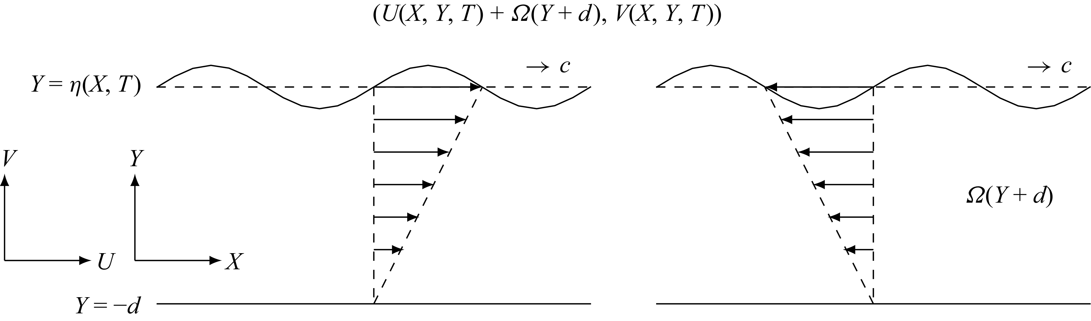
 c>0
c>0 Ω(Y+d)
 Y=−d
Y=−d Ω>0
Ω>0 Ω<0
Ω<0
 c^−ω(1+y)
 y∈[−1,0]
 c^>ω>0
 c^>0>ω
 0
0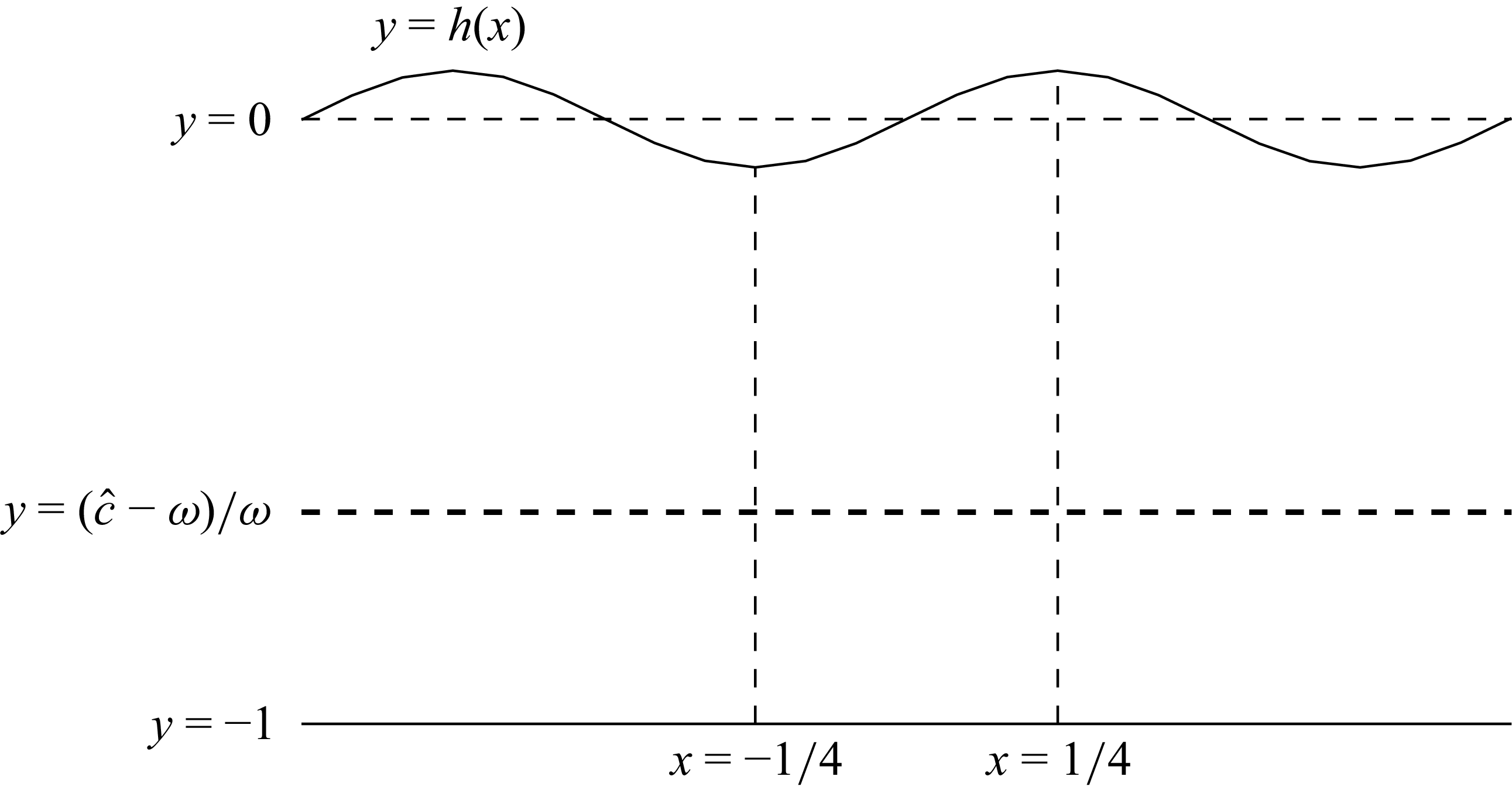
 c^
c^ h(x)=Asin(2πx)
 1
1 y=0
y=0 x=±(1/4)
 y=c^−ω/ω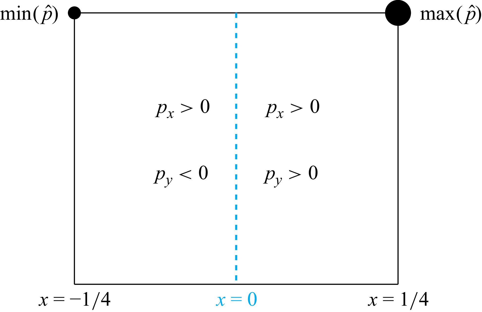
 p^
p^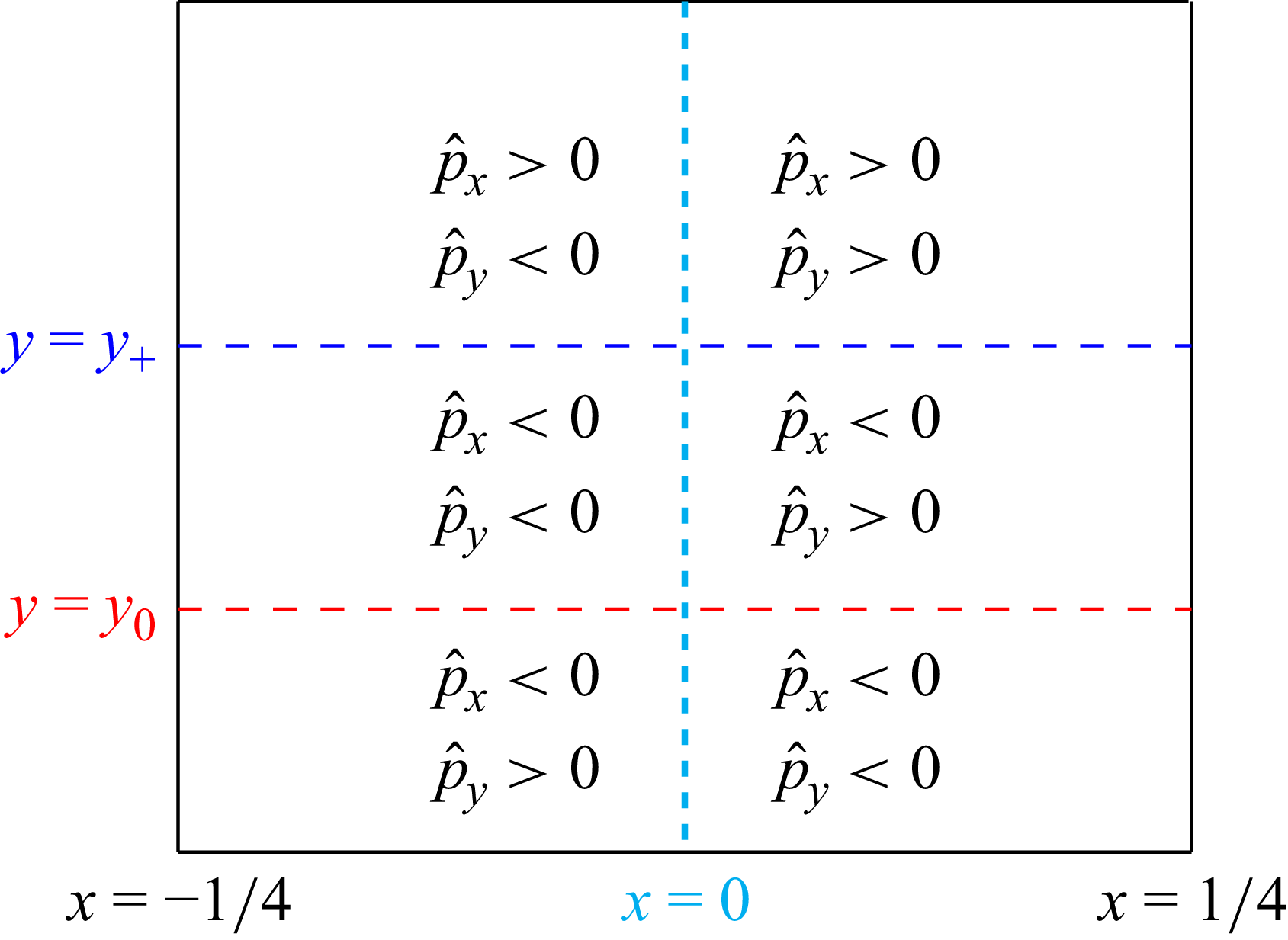
 p^
p^ y=0
y=0 y=−1
y=−1 ω>0
ω>0 y=y0∈(−1,0)
 p^x
p^x y=y+∈(y0,0)
 y+∈(y0,−1)
 p^y
p^y y=y0
y=y0 x=0
x=0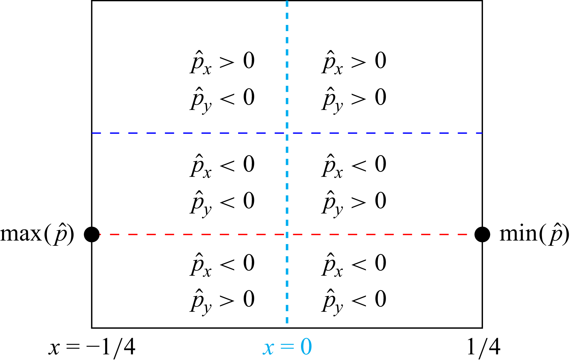
 p^
p^ ω>0
ω>0 y=y0
y=y0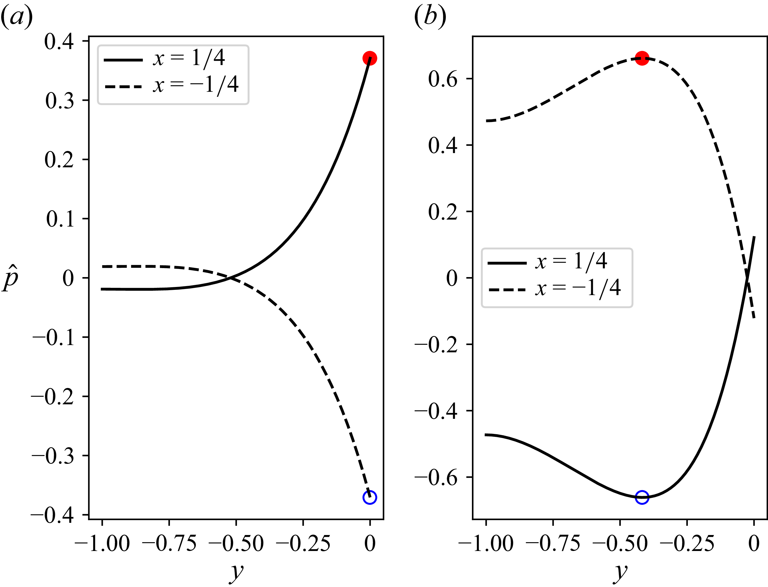
 x=±(1/4)
 δ=0.4
δ=0.4 a1=1
a1=1 γ1≈0.324
 0.6
0.6 9.8
9.8 38.9
38.9 δ
δ ω
ω ω2=1<38.9
 (−(1/4),0)
 (1/4,0)
 ω2≈39.1
 (1/4,y0)
 (−(1/4),y0)
 y0≈−0.42
 ω=1
ω=1 ω=39.1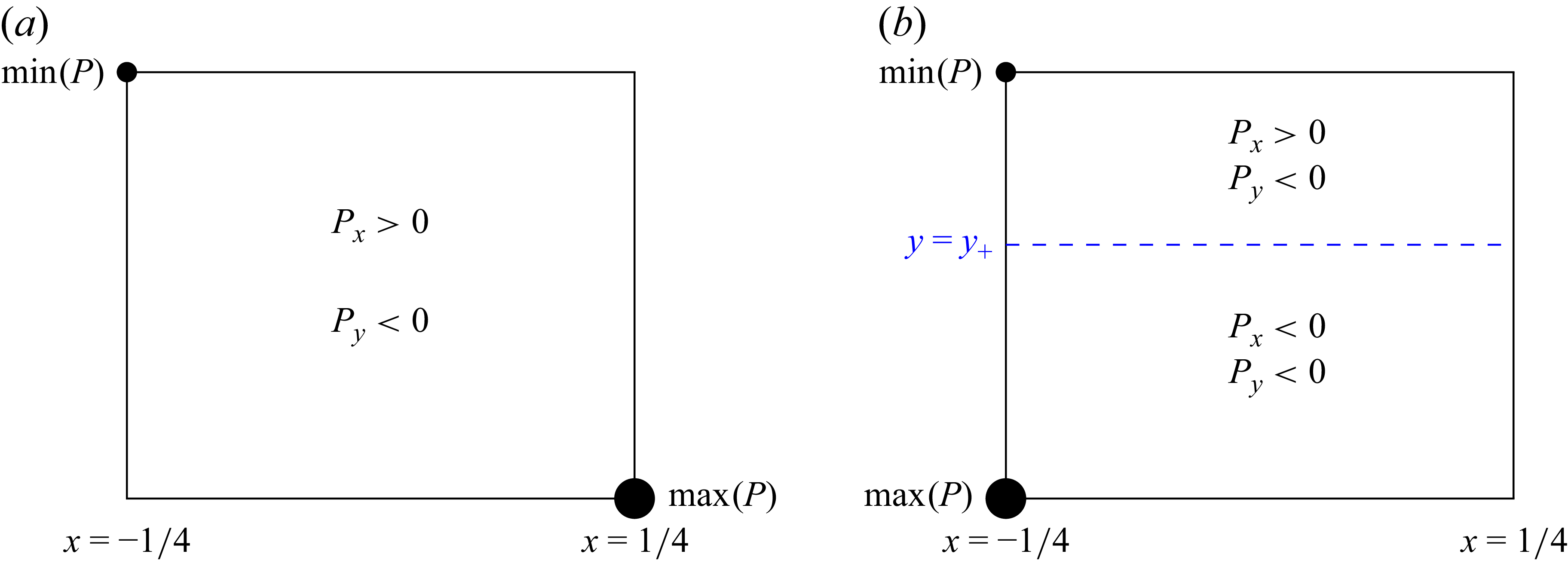
 y+
y+ Px(x,y+)=0
 y+
y+ [−1,0)
 Open access

