


1. Introduction
Spiral Poiseuille flow (SPF) refers to a system in which a fluid, confined in the gap between two concentric cylinders rotating at different angular velocities, is forced also by an axial pressure gradient. This set-up has received considerable attention owing to its relevance as building block flow to deepen the understanding of centrifugal and shear transition mechanisms in simple and controllable conditions. Most of the available studies refer to the application and development of stability theories that could be calibrated against flows characterized by Taylor-type supercritical instabilities and subcritical Tollmien–Schlichting (TS)-type instabilities.
The stability of SPF to axisymmetric perturbations in the narrow-gap limit has been investigated by Chandrasekhar (Reference Chandrasekhar1960, Reference Chandrasekhar1962), di Prima (Reference di Prima1960) and Hughes & Reid (Reference Hughes and Reid1968), who showed the stabilizing effect of the axial pressure gradient.
Chung & Astill (Reference Chung and Astill1977) were the first who removed the assumptions of axisymmetric perturbations and narrow gap ( $R_o - R_i \ll (R_o+ R_i)/2$, $R_i$ and $R_o$ being the inner and outer cylinder radii, respectively) still confirming an appreciable delay of the first Hopf bifurcation caused by the axial pressure gradient.
Takeuchi & Jankowski (Reference Takeuchi and Jankowski1981) further extended the previous results in the case of radius ratio  $\eta =R_i/R_o=0.5$, removing the assumption that the critical Taylor number monotonically increases with the Reynolds number, for all azimuthal wavenumbers. They further verified the applicability of the linear stability theory in determining the onset of a non-axisymmetric secondary flow using a few experimental tests, in a limited range of Reynolds numbers.
Ng & Turner (Reference Ng and Turner1982) significantly extended the Reynolds number range (based on the annular gap width  $D=R_o-R_i$ and the bulk velocity in the axial direction $U_b$) from $Re=100$ (Takeuchi & Jankowski Reference Takeuchi and Jankowski1981) up to $6000$ for $\eta = 0.77$ and $0.95$. The study confirmed the major role played by non-axisymmetric disturbances for $Re>20$ in the shape of the stability boundaries in the Reynolds–Taylor phase space.
Cotrell & Pearlstein (Reference Cotrell and Pearlstein2004) and Cotrell, Rani & Pearlstein (Reference Cotrell, Rani and Pearlstein2004) extended the analysis of Ng & Turner (Reference Ng and Turner1982) at higher Reynolds numbers, for  $\eta = 0.50, 0.77$ and $0.95$, up to the SPF instability to TS disturbances.
In more detail, for the narrow-gap case ( $\eta =0.95$) Cotrell et al. (Reference Cotrell, Rani and Pearlstein2004) demonstrated that on increasing the Reynolds number up to $Re^*=7716$ the critical azimuthal wavenumber increases up to $m_{crit}=149$; beyond $Re^*$, however, $m_{crit}$ abruptly drops to $2$. For $Re^*< Re< Re_{AP}$, $Re_{AP}$ being the value corresponding to the onset of TS-like instability in non-rotating annular Poiseuille flow ( $Re_{AP}=7739.5$), the critical azimuthal wavenumber gradually reduces to 0. Similar conclusions have been drawn also for $\eta = 0.77$ and $\eta =0.50$ for which the ( $Re^*,Re_{AP}$) pair becomes ( $8677,8883.3$) and ( $9916,10359$), respectively. However, in these last two cases, TS-like instability for $Re=Re_{AP}$ occurs in a non-axisymmetric fashion, namely $m_{crit}=1$ for $\eta = 0.77$ and $m_{crit}=2$ for $\eta = 0.50$. This result was anticipated for the $\eta =0.5$ case by Meseguer & Marques (Reference Meseguer and Marques2002) who investigated the effects of shear and centrifugal instability mechanisms on the topological features of the neutral stability curves.
Kaye & Elgar (Reference Kaye and Elgar1958) experimentally investigated the stability of SPF individuating the transitional Taylor number range for  $0\leq Re \leq 1000$ (respectively $0\leq Re \leq 900$) at $\eta =0.734$ (respectively $\eta =0.820$). Regardless of the $\eta$ value, $Ta_{tr}$ has been found to initially increase with $Re$, to attain a maximum and then to rapidly drop to zero for the largest Reynolds number ( $Re^{max}_{tr}=1000$ for $\eta =0.734$ and $Re^{max}_{tr}=900$ for $\eta =0.820$). The shape of the transitional boundary proposed by Kaye & Elgar (Reference Kaye and Elgar1958) was confirmed by Williamson (Reference Williamson1964) ( $\eta =0.90$) and Sorour & Coney (Reference Sorour and Coney1979) ( $\eta =0.80$ and $\eta =0.955$).
Figure 1 collects all the available experimental and numerical data for  $\eta >0.70$ reporting in the $Re$–
$Re$– $\hat {T}a$ plane the critical (Cotrell et al. Reference Cotrell, Rani and Pearlstein2004) and transitional (Kaye & Elgar Reference Kaye and Elgar1958; Williamson Reference Williamson1964; Sorour & Coney Reference Sorour and Coney1979) conditions. In figure 1 the modified Taylor number $\hat {T}a$ is defined as $\hat {T}a=Ta \sqrt {(1-\eta ) /\eta }$, where $Ta=\varOmega R_i\; D /\nu$, $\nu$ being the fluid kinematic viscosity. The use of $\hat {T}a$ is preferred to $Ta$ in the narrow-gap geometry, because it allows one to avoid the divergence of $Ta_{cr}$ occurring when $\eta \longrightarrow 1$, i.e. plane Couette (Orzag & Kells Reference Orzag and Kells1980). Indeed, while a good agreement between the experimental and theoretical results is generally observed for small Reynolds numbers, i.e $\hat {T}a_{cr}\sim \hat {T}a_{tr}$, the prediction of the stability theory ( $Re^{max}_{cr}=Re_{AP}\sim 10^4$) for the Reynolds numbers at which $\hat {T}a$ vanishes is one order of magnitude off with respect to the experimental findings ( $Re^{max}_{tr}\sim 10^3$).
Critical and transitional conditions. Lines (Cotrell et al. Reference Cotrell, Rani and Pearlstein2004): solid,  $\eta =0.950$; dashed, $\eta =0.770$. Circle (Sorour & Coney Reference Sorour and Coney1979): black, $\eta =0.80$; red, $\eta =0.955$. Right triangle (Williamson Reference Williamson1964): black, $\eta =0.90$. Left triangle (Kaye & Elgar Reference Kaye and Elgar1958): black, $\eta =0.734$; red, $\eta =0.802$.

A possible explanation for these discrepancies has been offered by Heaton (Reference Heaton2008) who investigated the SPF problem for a large-gap geometry ( $\eta =0.5$) in both the co-rotating and counter-rotating cases solving the linearized three-dimensional Navier–Stokes equations and analysing the transient growth of the optimal disturbance. He has shown that at high Reynolds number, small disturbances superposed on the laminar SPF undergo a strong transient growth leading to the formation of elongated spanwise modulations of the axial velocity (streaks). Therefore, the laminar to turbulent transition occurs via streamwise streak generation and growth (lift-up effect) in a by-pass transition scenario, rather than through a classical centrifugal instability modes mechanism.
All the studies mentioned above aimed at identifying the stability boundaries in the  $Re$–
$Re$– $Ta$ plane for SPF: this is definitely useful information for fundamental questions although their validity for the determination of the actual transitional conditions is rather limited. Yamada (Reference Yamada1962a,Reference Yamadab) carried out a set of experiments to analyse torque and friction coefficients of SPF in several narrow-gap geometries, covering both laminar and turbulent conditions. Using these measurements, Yamada (Reference Yamada1962a,Reference Yamadab) identified, for radius ratios $\eta =0.97$, $0.98$ and $0.99$, the transitional boundary in the $Re$–
$Re$– $Ta$ plane, confirming the order of magnitude of $Re^{max}_{tr}$ found by Kaye & Elgar (Reference Kaye and Elgar1958), Williamson (Reference Williamson1964) and Sorour & Coney (Reference Sorour and Coney1979). Moreover, for moderate values of the Taylor number ( $Ta<5000$) and provided the Reynolds number is sufficiently high ( $Re \sim 10^4$), it has been shown that the friction coefficient obeys the Blasius turbulent correlation $\lambda _B=0.26 Re^{-0.24}$. Keeping $Ta$ fixed and reducing $Re$, the mechanism inducing the reverse transition from turbulent to laminar flow strongly depends on the Taylor number. Indeed, the rotation of the inner cylinder substantially reduces the Reynolds number at which the reverse transition sets in.
Despite the wealth of theoretical, experimental and numerical studies available in the literature, the discrepancies concerning the shape of critical and transitional boundaries in the  $Re$–
$Re$– $Ta$ plane at high Reynolds numbers in a SPF, and in particular the possibility of having sustained turbulence in subcritical flow conditions, still remain unexplained. Important contributions to clarify these issues and to unravel the mechanisms promoting the occurrence of the reverse transition may come from direct numerical simulations (DNS), and the present study is motivated by this statement. We present the results of DNS carried out in a narrow-gap geometry for the flow parameters of Yamada (Reference Yamada1962a,Reference Yamadab). The data, coming from a spectrally accurate DNS, may contribute to clarifying the discrepancies between the theoretical critical values and the experimental transitional ones. In particular, the role played by the finite size fluctuating velocity components in determining the suppression of the turbulence activity is evidenced through a three-dimensional dumping mechanism. To this aim, the key is the characterization of the turbulent inner layer statistics, which is performed by identifying the turbulence structure using the Reynolds stress tensor and the corresponding budgets.
The article is organized as follows. The problem formulation with the governing equations and run parameters are reported in § 2, while a short description of the numerical method is given in § 3. The discussion of the results, in terms of both global and local quantities, is provided in § 4 and closing remarks are given in § 5. Details concerning the adequacy of the computational domain and spatial resolution can be found in the Appendix.
2. Problem formulation
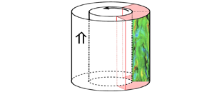
We consider an incompressible, viscous flow between two concentric cylinders; the inner one, of radius  $R_i$, is rotating with angular velocity $\varOmega$, while the outer one, of radius $R_o$, is at rest. The cylinders have an axial length $L_z$, and the flow is assumed periodic in this direction which is forced by a constant pressure gradient (figure 2). The variables are made dimensionless using the tangential velocity of the inner cylinder $W_i=\varOmega R_i$ and the gap width $D=R_o-R_i$. The geometry is completely defined by the pair $\eta =R_i/R_o$, $\ell _z=L_z/D$ and the flow is fully characterized by the Taylor and Reynolds numbers:
 \begin{equation} Ta=\frac{ W_i D}{\nu}, \quad Re=\frac{U_b D}{\nu}, \end{equation}
with  $U_b$ the bulk axial velocity.

Run matrix of the simulations at  $Ta=1500$, $\eta =0.98$, dimensions of the computational domains in inner and outer coordinates and colour code for the lines used to report the results.

The governing equations are the incompressible Navier–Stokes equations which in primitive variables and dimensionless form read
 \begin{equation} \frac{{\partial {\boldsymbol u}} }{{\partial t}} ={-} \boldsymbol{\nabla} p - {\mathcal{N}} {\boldsymbol u} +\frac{1}{Ta}{\mathcal{L}} {\boldsymbol u}+ {\mathcal{F}},\quad \boldsymbol{\nabla} \boldsymbol{\cdot} {\boldsymbol u} = 0, \end{equation}
with  ${\boldsymbol u} =(u, v,w)=(u_1, u_2,u_3)$ the axial ( $z$), radial ( $r$) and azimuthal ( $\theta$) velocity components, respectively, and $p$ the pressure.
In (2.2)  ${\mathcal {L}} {\boldsymbol u}$ and ${\mathcal {N}} {\boldsymbol u}$ indicate the diffusive and convective terms, respectively. The specific volume force ${\mathcal {F}}=({\mathcal {F}}_z,0,0)$ represents the applied (negative) pressure gradient to induce an axial flow (in the positive $z$ direction). The imposed boundary conditions are ${\boldsymbol u} =(0, 0, 1)$ and ${\boldsymbol u} =(0, 0, 0)$ at the inner and outer surfaces, respectively.
The performance of SPF is usually defined in terms of the following torque  $C_{\tau }$ and axial friction $\lambda$ coefficients:
 \begin{gather} C_\tau={-} \frac{T_{R\theta,i}}{\rho W_i^2} ={-}\frac{r_i}{Ta} \frac{{\rm d}}{{\rm d} r}\left (\frac{ w}{r}\right)_{r_i}, \end{gather}
 \begin{gather} \lambda=\frac{ 8}{\rho U_b^2} \frac{ {T}_{RZ,i}\, R_i- {T}_{RZ,o} \, R_o }{R_o+R_i}= \frac{8}{1+\eta} \frac{Ta}{Re^2}\left[ \left(\frac{{\rm d} u}{{\rm d}r}\right)_{r_i} \eta - \left(\frac{{\rm d} u}{{\rm d}r}\right)_{r_o} \right], \end{gather}
where  $T_{R\theta,i}$ is the azimuthal component of the wall shear stress at the inner cylinder and $T_{RZ,i/o}$ are the analogous axial components of the shear stress at the inner/outer cylinders.
For Taylor and Reynolds numbers within the stability boundaries of figure 1, the following exact solution holds:
 \begin{equation} \left. \begin{aligned} u\left(r \right) & = \displaystyle{ 2 \frac{Re}{Ta} \frac{ \left[ 1- r^2 \left(1-\eta\right)^2 \right] \log{\eta} - \log{\left[r \left(1-\eta\right) \right] } \left(1 - \eta^2\right)} {\left(1 + \eta^2\right) \log{\eta} + \left(1 - \eta^2\right) } },\\ v\left(r \right) & = \displaystyle{0},\\ w\left(r \right) & = \displaystyle{ \frac{\eta}{1-\eta^2} \left[ \frac{1}{r\left(1-\eta\right)} - r \left(1-\eta\right) \right]}. \end{aligned} \right\} \end{equation}
 The corresponding expressions of torque  $C_{\tau }$ and axial friction $\lambda$ coefficients in terms of $Re$,
$Re$,  $Ta$ and $\eta$ read
 \begin{gather} C_{\tau,C}=\frac{2}{Ta} \frac{1}{\eta\left(1+\eta\right)}, \end{gather}
 \begin{gather} \lambda_P=\frac{32}{Re} \frac{\left(1-\eta\right)^2} {1+\eta^2 +\dfrac{1-\eta^2}{\log{\eta}} }. \end{gather}
As shown in figure 1, the boundaries of the region in which the solution (2.5) applies are neat and well defined at small Taylor and Reynolds numbers whereas they become blurred when the Reynolds number increases and so does the precise location of the transitional boundary. Nevertheless, the experimental data of Yamada (Reference Yamada1962a,Reference Yamadab) give a clear picture of the reverse transition process occurring when the axial Reynolds number is progressively decreased. Figure 3, reporting  $C_{\tau }$ and $\lambda$ from Yamada (Reference Yamada1962a,Reference Yamadab) for $\eta \sim 0.98$ and $Ta=1500$, evidences the smoothness of the process, highlighting the differences between rotating and non-rotating cases. Specifically, in the $Ta=0$ case, figure 3(b) shows that when $Re$ is reduced below $\simeq 3400$, the friction coefficient drops below the turbulent Blasius correlation and smoothly approaches the laminar value when $Re \le 1500$. The latter value is considerably smaller than the Reynolds number associated with the TS-like instability in non-rotating annular Poiseuille flow ( $Re_{AP}$): according to Garg (Reference Garg1980), at $\eta =0.98$, the result is $Re_{AP}\simeq 7700$. Conversely in the rotating case, starting from $Re \simeq 2900$, the reduction of the Reynolds number leads to a gradual departure from the turbulent Blasius power law before approaching the laminar value at $Re\simeq 850$. Moreover, the extent of the Reynolds-number range in which the reverse transition process occurs is seen to be larger in the rotating case compared with the non-rotating one. At Taylor number values higher than 1500 the situation becomes considerably more involved (Yamada Reference Yamada1962a,Reference Yamadab) and worth further investigation.
Torque (a) and friction (b) coefficients versus Reynolds number (Yamada Reference Yamada1962a,Reference Yamadab): square,  $Ta=0$; circle, $Ta=1500$. Red vertical lines and red circles denote present numerical data.

The study of mechanisms through which the reverse transition process takes place in SPF is the main aim of the present study. The comprehension of the mechanisms routing a turbulent flow to a laminar state in a smooth manner may open a way to the exploitation of flow-control procedures with huge fundamental and practical outcomes.
In the present study, SPF in a narrow-gap geometry with  $\eta =0.98$ is considered. Keeping fixed the Taylor number ( $Ta=1500$), a database consisting of five highly resolved DNS has been generated. Starting from sustained turbulent conditions, the Reynolds number has been progressively reduced until complete relaminarization. Table 1 reports the Reynolds numbers of the investigated cases, indicated by red vertical lines in figure 3.
3. Numerical method and computational set-up
Equations (2.2) have been numerically integrated using a pressure correction scheme (van Kan Reference van Kan1986) with a spectral multi-domain discretization (Manna & Vacca Reference Manna and Vacca1999). In the axial and azimuthal directions a blended Fourier decomposition has been used while in the radial direction a pseudo-spectral technique, improved through a multi-domain approach with patching interfaces, has been employed. The whole algorithm has been extensively validated in both steady (Manna & Vacca Reference Manna and Vacca2001, Reference Manna and Vacca2009) and unsteady (Manna, Vacca & Verzicco Reference Manna, Vacca and Verzicco2012, Reference Manna, Vacca and Verzicco2015, Reference Manna, Vacca and Verzicco2020) turbulent flows.
For each run, table 1 reports the axial and azimuthal lengths in inner coordinates  $\ell ^+=L/\delta ^+$, with the viscous length scale $\delta ^+ = \nu /u_\tau$. The friction velocity $u_\tau$ is computed on the basis of the surface-averaged wall shear stress $\tau _{rz}$, which is then long-time-averaged. Additionally, the surface-averaged $\tau _{rz}$ is built using the inner and outer wall data, i.e. $\tau _{rz}=(\tau _{rz,i} \,r_i+\tau _{rz,o} \,r_o)/ (r_i+r_o)$. The predominance of $\tau _{rz}$ over $\tau _{r\theta }$ is addressed in the next section. The axial and azimuthal lengths of the computational domain have been chosen to accommodate the largest flow coherent structures and the adequacy of the domain size has been verified through the analysis of the two-point correlation at various distances from the walls: for the sake of conciseness in the Appendix only the correlations for the velocity components at $y^+=(r-r_i)/\delta ^+=5$ are reported in both axial and azimuthal directions.
The computational domain has been radially split into 11 subdomains ( $N_{sub}= 11$), whose width in the radial direction has been devised to enhance the wall-layer resolution. The sizes of the subdomains, given as percentages of the gap, are the following: $2.5\,\%, 2.5\,\%, 5\,\%, 10\,\%, 20\,\%, 20\,\%, 20\,\%, 10\,\%, 5\,\%, 2.5\,\%, 2.5\,\%$. The simulations of the R1 and R2 cases have been carried out setting the number of modes in each subdomain equal to $N_r=15$, $N_z=256$ and $N_{\theta }=144$, in the radial, axial and azimuthal directions, respectively. To keep the resolution approximately constant, the number of modes in all directions, in the remaining tests, has been changed.
Additional details of the resolution, together with the maximum azimuthal spacing  $(r \Delta \theta )^+_{max}$ and the distance from the wall of the first interior point $y^+_w$, can be found in table 2.
Discretization parameters.

The R1–R4 cases have been initialized starting from the large-eddy simulation fields of Manna & Vacca (Reference Manna and Vacca2007) interpolated on finer grids. The R5 case has been run starting from the R4 case. In particular, a preliminary mapping procedure has been applied to account for the necessity of increasing the computational domain lengths. Therefore, the source term  ${\mathcal {F}}_z$ in (2.2) has been modified in order to reproduce a condition in which the reverse transition process has been experimentally predicted by Yamada (Reference Yamada1962a,Reference Yamadab) (figure 3). We anticipate that in the R5 case, the volume-averaged turbulent kinetic energy shows a monotonic decrease in time leading finally to the destruction of all large- and small-scale structures.
Numerical results have been obtained processing  $1500$ statistically independent fields separated in time by $0.12$ dimensionless units $D/u_\tau$. Data were collected only once constant time- and space-averaged wall shear stresses were achieved. All quantities are space-averaged in the homogeneous $z$ and $\theta$ directions.
In the following, as usual for turbulent flows, we denote with an overline all quantities averaged in time and over the two homogeneous  $z$ and $\theta$ directions. The deviation of the instantaneous values from the averaged quantities is indicated by a prime symbol.
4. Results
4.1. Global parameters
The overall flow dynamics is analysed in terms of torque  $(C_\tau )$ and axial friction ( $\lambda$) coefficients defined in (2.3) and (2.4), having replaced the shear stresses and velocities with their surface- and time-averaged values.
Table 3 reports the relevant global parameters characterizing the investigated cases, and we start from a discussion of the R1 run. The main features of the axial flow are not affected by the rotation of the inner cylinder, as is evident from the friction coefficient which agrees with the Blasius value (figure 3b). This is confirmed also by the ratio of the maximum ( $U_m$) and bulk ( $U_b$) velocities which agrees very well with the Dean correlation (Dean Reference Dean1978): $U_m/ U_b = 1.28 Re^{-0.0116}= 1.16$. While the axial flow is unaffected by the inner cylinder rotation, the axial pressure gradient strongly modifies the Taylor vortices, thus suggesting a ‘one-way’ coupling of the azimuthal to the axial momentum components. Indeed, the torque coefficient $C_\tau$ more than doubles with respect to the pure Taylor flow ( $C_{\tau,0}=2.03 \times 10^{-3}$; Manna & Vacca Reference Manna and Vacca2009). The effects of the axial pressure gradient on the topology of the cross-flow in the $r$–
$r$– $z$ plane can be appreciated with the help of figure 4, showing, in outer coordinates, the instantaneous velocity vectors $(v^\prime, u^\prime )$ superposed on the $w^{\prime }$ scalar field. The changes of the vortex structures increasing the Reynolds number from $Re=0$ to $Re=5766$ evidence the effect of the combined flow which mixes azimuthal and axial shear at the boundaries and results in smaller flow scales.
Instantaneous velocity vectors  $(v^\prime, u^\prime )$ in the cross-plane at $Ta=1500$ superposed on the $w^{\prime }$ scalar field, in outer coordinates, for (a) $Re=0$ (Manna et al. Reference Manna, Vacca and Verzicco2020) and (b) $Re=5766$.

Global parameters.

A reduction of  $Re$ below $5766$ leads to a monotonic increase of the $U_m/ U_b$ ratio. For Reynolds numbers smaller than $2858$, the friction coefficient always exceeds the Blasius value and the difference increases as the Reynolds number is reduced (figure 3b). On the other hand, starting from R1, the torque coefficient is a continuously decreasing function of $Re$ up to the relaminarization of R5 (figure 3a). In the R4 case, $C_\tau$ is smaller than the value pertaining to the pure Taylor–Couette flow $C_{\tau,0}$. When the lowest Reynolds number is attained (R5) both friction and torque coefficients agree well with the Couette–Poiseuille values ( $C_{\tau,C}=0.69 \times 10^{-3}$ and $\lambda _P=6.48 \times 10^{-2}$; (2.6) and (2.7)). Therefore, the complete relaminarization of the flow field has occurred, in agreement with the experimental findings of Yamada (Reference Yamada1962a,Reference Yamadab), as shown in figure 3. Incidentally, we observe that for all cases the ratio $\overline {\tau }_{rz,i}/\overline {\tau }_{rz,o}$ (table 3) is always close to unity owing to the narrow-gap geometry ( $\eta =0.98$). Finally, table 3 shows that the vector sum $\overline {\tau }_{tot}$ of $\overline {\tau }_{rz}$ and $\overline {\tau }_{r\theta }$ is always very close to $\overline {\tau }_{rz}$.
Figure 5(a) reports in inner coordinates the radial profiles of the time-averaged axial velocity component: regardless of the Reynolds number, within the viscous sublayer  $y^+ < 5$, all velocity profiles follow the law $\bar {u}^+=y^+$. At the highest Reynolds number (R1), for $y^+> 30$ the mean velocity profile is well represented by the logarithmic law, while on reducing $Re$, the logarithmic layer becomes progressively less neat. The overlapping between the velocity profile of the R5 case with (2.5) confirms that at this Reynolds number the flow is laminar.

The radial profiles of the time-averaged azimuthal velocity component are shown in figure 5(b), as a function of the distance from the inner wall  $y=r-r_i$. For the sake of comparison the laminar (2.5) and pure Taylor–Couette (Manna & Vacca Reference Manna and Vacca2009) distributions also are reported. The main effect of the axial pressure gradient is the slope reduction of the velocity profiles at the walls, until the Couette distribution is recovered for the R5 run. In all cases the radial profile of $\bar {w}$ shows a significant departure from the pure Taylor–Couette flow, even in the R3 case whose torque coefficient differs only slightly from $C_{\tau,0}$. All $C_{\tau }$ values appear to be considerably smaller than the corresponding $\lambda$ values, and so are the corresponding wall shear stresses, on account of the $U_b/W_i$ ratios (see table 3).
Figure 6 shows the radial distribution of turbulence intensities in inner coordinates. As the axial pressure gradient decreases, both the axial and radial intensities monotonically decay in the wall region. Figure 6(c) indicates that the reduction of the Reynolds number first leads to a uniform attenuation of  $\sqrt {\overline {w^\prime w^\prime }}^+$ (from R1 to R2) and then to an increase (from R2 to R4). There is a twofold explanation for such a behaviour: an alteration of the turbulence production terms along with a modified Reynolds stresses redistribution mechanism in the energy budgets. This issue is addressed later on.
Radial distribution of  $\sqrt {\overline {u^\prime u^\prime }}$ (a), $\sqrt {\overline {v^\prime v^\prime }}$ (b) and $\sqrt {\overline {w^\prime w^\prime }}$ (c) in inner coordinates. Line colours as in table 1: black solid line, R1; red solid line, R2; green solid line, R3; blue solid line, R4.

We now turn to the analysis of the viscous  $\boldsymbol {\tau }^v$ and turbulent $\boldsymbol {\tau }^t$ stresses. To this aim we consider axial and azimuthal components of the momentum equation (2.2) averaged in the homogeneous directions:
 \begin{gather} 0={-} \frac{1}{r} \frac{{\rm d} \left(\overline{u^\prime v^\prime}\; r\right)}{{\rm d}r} +\frac{1}{r} \frac{{\rm d}\left(\overline{\tau}_{rz} r\right)}{{\rm d}r}+ {\mathcal{F}}_z \quad \text{with} \ \overline{\tau}_{rz}=\frac{1}{Ta} \frac{{\rm d} \bar{u}}{{\rm d}r}, \end{gather}
 \begin{gather} 0={-}\frac{{\rm d}\overline{v^\prime w^\prime}}{{\rm d}r} - 2 \frac{\overline{v^\prime w^\prime}}{r} + \frac{{\rm d} \overline{\tau}_{r \theta}}{{\rm d}r} +\frac{2}{r} \overline{\tau}_{r\theta}\quad\text{with} \ \overline{\tau}_{r\theta}=\frac{r}{Ta} \frac{{\rm d} }{{\rm d}r} \left(\frac{\bar{w}}{r}\right). \end{gather}
Integrating equation (4.1) across the gap, the following expression for the axial pressure gradient is obtained:
 \begin{equation} {\mathcal{F}}_z = 2 \frac{\overline{\tau}_{rz,o} \, r_o -\overline{\tau}_{rz,i} \, r_i }{r_o^2 -r_i^2}. \end{equation}
 The radial distributions of the total stresses  $\tau ^t_z+\tau ^v_z$ and $\tau ^t_\theta +\tau ^v_\theta$ are obtained by integrating equations (4.1) and (4.2), respectively:
 \begin{gather} \underbrace{-\overline{u^\prime v^\prime}}_{\tau^t_z} +\underbrace{\frac{1}{Ta} \frac{{\rm d} \bar{u}}{{\rm d}r}}_{\tau^v_z}= \frac{{\mathcal{F}}_z}{2}\left( \frac{r_i^2}{r}-r\right)+ \frac{r_i}{r}\tau^v_{z,i}, \end{gather}
 \begin{gather} \underbrace{- \left[\overline{v^\prime w^\prime} +2\int_{r_i}^r \frac{\overline{v^\prime w^\prime} }{r} \,{\rm d}r\right]}_{\tau^t_\theta}+ \underbrace{\frac{1}{Ta}\left[r \frac{{\rm d} }{{\rm d}r} \left(\frac{\bar{w}}{r}\right)+ 2 \left(\frac{\bar{w}}{r}-\frac{1-\eta}{\eta} \right)\right]}_{\tau^v_\theta} =\tau^v_{\theta,i}. \end{gather}
 Figure 7(a) reports the turbulent shear stress  $\tau _{z}^t$, with the viscous $\tau _{z}^v$ and total $(\tau _{z}^t+\tau _{z}^v )$ ones, normalized by $\tau ^v_{z,i}$, across the gap in inner coordinates. Regardless of the Reynolds number, the total stress shows a linear trend. Indeed, the curvature is not effective in causing a departure from linear behaviour, as suggested by (4.4). Moreover, the viscous stress profiles collapse onto a single curve for $y^+ < 10$, as expected in inner scaling. Finally, figure 7(a) evidences a gradual reduction of the turbulent term, similarly to that reported in figures 6(a) and 6(b) when discussing the $\sqrt {\overline {u^\prime u^\prime }}^+$ and $\sqrt {\overline {v^\prime v^\prime }}^+$ distributions. On account of the axial velocity profiles reported in figure 5(a), an attenuation of the turbulent production driven by the axial mean shear is expected: this is discussed in detail in the following part.
Radial distribution of turbulent  $\tau _{z}^t/ \tau ^v_{z,i}$ (dashed lines), viscous $\tau _{z}^v/ \tau ^v_{z,i}$ (dash-dotted lines) and total $(\tau _{z}^t+ \tau _{z}^v)/ \tau ^v_{z,i}$ (solid lines) stresses in inner coordinates (a); turbulent $\tau _{\theta }^t/ \tau ^v_{\theta,i}$ (dashed lines) and viscous $\tau _{\theta }^v/ \tau ^v_{\theta,i}$ (solid lines) stresses in inner coordinates (b). The inset shows the same quantities in outer coordinates throughout the whole domain. Line colours as in table 1: black solid line, R1; red solid line, R2; green solid line, R3; blue solid line, R4.

Figure 7(b), reporting in inner coordinates the radial distribution of  ${\tau }_{\theta }^t$ and ${\tau }_{\theta }^v$, normalized by $\tau ^v_{\theta,i}$, shows that, in the bulk region, lowering the axial Reynolds number induces an appreciable reduction of the turbulent part accompanied by a corresponding increase of the viscous contribution. Both turbulent and viscous stresses collapse onto a single curve for $y^+ < 15$. Thus, while the wall layer is mostly governed by the Taylor number, the outer layer is controlled by $Re$.
$Re$.
According to Frohnapfel et al. (Reference Frohnapfel, Lammers, Jovanovic and Durst2007), the process of turbulent to laminar transition in a plane channel geometry is dominated by a modification of the near-wall turbulent structures which have been shown to become more elongated in the streamwise direction. Simultaneously, the Reynolds stress tensor components become more uneven in the sense that the axial turbulence intensity  $\overline {u_1^\prime u_1^\prime }$ prevails over the other two components. Quantitatively this can be seen by analysing the diagonal terms of the anisotropy Reynolds stress tensor which, using the notation $(u_1^\prime, u_2^\prime,u_3^\prime ) =(u^\prime, v^\prime,w^\prime )$, reads as follows:
 \begin{equation} b_{ij}=\frac{ \overline{u_i^\prime u_j^\prime}} {\overline{u_i^\prime u_i^\prime}} -\frac{1}{3}\delta_{ij}. \end{equation}
In the above equation,  $\overline {u_i^\prime u_i^\prime }$ equals twice the turbulent kinetic energy. If one of the diagonal components $b_{ii}$ is positive, the corresponding normal stress is larger than the average of the other normal stresses and the turbulence becomes more anisotropic (essentially one-dimensional when $b_{ii}=2/3$). On the other hand, a single negative $b_{ii}$ value indicates a tendency towards two-dimensional turbulence, with the $i$th component significantly smaller than the sum of the other two in the limit of $b_{ii}=-1/3$ (Marchis, Napoli & Armenio Reference Marchis, Napoli and Armenio2010).
Figure 8 shows the  $b_{ii}$ radial distribution in inner coordinates of R2 (figure 8a), R3 (figure 8b) and R4 (figure 8c), taking R1 as reference. The reduction of the Reynolds number from R1 to R2 leads to an increase (in magnitude) of all diagonal terms revealing an enhanced anisotropy of the turbulence scales. Let us stress that the increase in magnitude of a negative quantity means that the latter is becoming more negative, i.e. a reduction is taking place. A further reduction of $Re$ (see figure 8b,c) implies a clear tendency towards a reduction (in magnitude) of $b_{11}$ and $b_{33}$, while $b_{22}$ remains essentially unaltered. Overall, a return to isotropy of the turbulence scales is taking place. It is worth noticing that in the R4 case a sign change of $b_{33}$ occurs for $y^+> 40$ and therefore $\overline {u_3^\prime u_3^\prime }$ exceeds the average of $\overline {u_1^\prime u_1^\prime }$ and $\overline {u_2^\prime u_2^\prime }$ .
Radial distribution of  $b_{ii}$ in inner coordinates, taking R1 as reference: (a) R2; (b) R3; (c) R4. Line colours as in table 1: black solid line, R1; red solid line, R2; green solid line, R3; blue solid line, R4.

An exhaustive characterization of the wall-layer turbulence structure in terms of deviation from the isotropic state requires the inspection of all components of the anisotropy Reynolds stress tensor. This information is efficiently condensed in the  $AI$ index (Manna et al. Reference Manna, Vacca and Verzicco2012):
 \begin{equation} AI=\frac{ II}{II_{1D}}, \end{equation}
with  $II$ the second invariant of the $b_{ij}$ tensor and $II_{1D}=-1/3$ the corresponding one-component turbulence value. Figure 9 reports in inner coordinates the radial distribution of $AI$ for all cases. For the sake of comparison, the plane channel data of Iwamoto, Suzuki & Kasagi (Reference Iwamoto, Suzuki and Kasagi2002), as reported in Iwamoto (Reference Iwamoto2002), are shown in figure 9(b).
Radial distribution of anisotropy index  $AI$ in inner coordinates. $(a)$ Spiral Poiseuille flow. Line colours as in table 1: black solid line, R1; red solid line, R2; green solid line, R3; blue solid line, R4. $(b)$ Turbulent plane channel (data of Iwamoto et al. (Reference Iwamoto, Suzuki and Kasagi2002), as reported in Iwamoto (Reference Iwamoto2002)): black solid line, $Re_\tau =300$; red solid line, $Re_\tau =150$; green solid line, $Re_\tau =110$.

Recall that a vanishing  $AI$ corresponds to three-dimensional, isotropic turbulence while $AI \rightarrow 1$ indicates turbulent fluctuations developing in one preferred direction (one-dimensional turbulence). Figure 9 supports the results reported in figure 8 showing that the reduction of the Reynolds number from 5766 to 2858 yields a nearly uniform anisotropy increase in the whole wall layer, while a further reduction of $Re$ has the opposite effect of increasing the isotropy. While the first trend is expected, being representative of pressure-driven flows as the driving force is reduced (see figure 9b), the latter is peculiar to SPF, where energy is added to the bulk flow through two different mechanisms, operating along orthogonal directions. As a result, the turbulence intensities are fed by two production terms, along with the inter-component energy transfer terms, whose effectiveness changes as $Re$ is reduced. Therefore, the comprehension of the energy redistribution mechanisms requires an analysis of the Reynolds stress budgets.
For the problem under investigation, the time-averaged energy budget of the axial variance is the most relevant whenever the  $Re/Ta$ ratio is considerable, as in the R1 and R2 cases. In these flows, most of the turbulent kinetic energy is contributed by the production term in the axial direction. Reducing the Reynolds number, both the shear stress and the axial mean shear uniformly attenuate, as previously shown in figure 7(a). To inspect the modification of the production term we present in figure 10 the time-averaged energy budget of the axial variance, which reads
 $$\begin{gather} \underbrace{-2 \overline{ u^\prime v^\prime } \frac{d \bar{u}}{dr}}_{P_{zz}} \underbrace{-\frac{1}{r} \frac{\partial \overline{ \left(r {u^\prime}^2 v^\prime\right)} }{\partial r} }_{T_{zz}} + \underbrace{\frac{1}{Re}\frac{1}{r} \frac{\partial}{\partial r} \left( r \frac{\partial \overline{{u^\prime}^2}}{\partial r}\right) }_{D_{zz}} + \underbrace{2 \overline{p^\prime \frac{\partial u^\prime}{\partial z}} }_{\varPi_{zz}}\nonumber\\ \underbrace{- \frac{2}{Re} \left[ \overline{ \left(\frac{\partial u^\prime}{\partial r}\right)^2+ \frac{1}{r^2} \left(\frac{\partial u^\prime}{\partial \theta}\right)^2+ \left(\frac{\partial u^\prime}{\partial z}\right)^2} \right] }_{-\epsilon_{zz}}=0. \end{gather}$$
Axial velocity fluctuation energy budget in inner coordinates: (a) R1 case, (b) R2 case, (c) R3 case and (d) R4 case. Black solid line,  $P_{zz}$; red solid line, $-\epsilon _{zz}$; green solid line, $T_{zz}$; blue solid line, $D_{zz}$; magenta solid line, $\varPi _{zz}$; black dashed line, $U_{zz}$.

In (4.8)  $P_{zz}$, $T_{zz}$, $D_{zz}$, $\varPi _{zz}$ and $-\epsilon _{zz}$ indicate production, turbulent transport, viscous diffusion, velocity–pressure gradient and dissipation, respectively. Figure 10 reports the radial distribution of all these terms along with their unbalance ( $U_{zz}$), in inner coordinates. Before proceeding any further let us recall that the velocity scale used to normalize all terms in the energy budget is based on the surface-averaged wall shear stress $\overline {\tau }_{rz}$. While approximate, this is a valid choice because the vector sum of $\overline {\tau }_{rz}$ and $\overline {\tau }_{r\theta }$ is very close to $\overline {\tau }_{rz}$ (see table 3). Close to the wall, $D_{zz}$ is positive and balances the dissipation. For $y^+ >30$, the production is essentially balanced by the sum of dissipation and velocity–pressure gradient, with negligible $T_{zz}$ and $D_{zz}$. In the present normalization, the scaling is only marginal as $Re$ is reduced by a factor of four. Indeed, the Reynolds-number reduction induces a uniform decrease (in magnitude) of all terms. Of interest for the comprehension of the transitional region widening is the rapid attenuation of $\varPi _{zz}$ as it governs the energy transfer among the normal stresses. Additionally, inspection of the velocity–pressure gradient term will allow substantiation of the peculiar behaviour of the anisotropy index in the wall layer, as $Re$ is reduced.
Let us split the velocity–pressure gradient  $\varPi _{ii}$ into the pressure strain $\varPhi _{ii}$ and pressure diffusion $\varPsi _{ii}$ terms as follows:
 \begin{equation} \left. \begin{aligned} \varPi_{zz} & =\varPhi_{zz}+\varPsi_{zz}= 2\overline{p^\prime \frac{\partial u^\prime} {\partial z}} + 0,\\ \varPi_{rr} & =\varPhi_{rr}+\varPsi_{rr}= 2\overline{p^\prime \frac{\partial v^\prime} {\partial r}} -2 \overline{ \frac{\partial \left(p^\prime v^\prime\right)} {\partial r}},\\ \varPi_{\theta\theta} & =\varPhi_{\theta\theta}+\varPsi_{\theta\theta}= \frac{2}{r} \overline{p^\prime \left( \frac{\partial w^\prime}{\partial \theta} +v^\prime\right)} - 2 \overline{ \frac{ p^\prime v^\prime} { r}}. \end{aligned} \right\} \end{equation}
 Owing to the free divergence constraint, only the diagonal pressure-strain terms  $\varPhi _{ii}$ produce an energy exchange among the velocity components. A negative (positive) value of $\varPhi _{ii}$ indicates an energy loss (gain) from the $i$th component towards the others. In a pure axial shear flow ( $Ta=0$), the production term exists only for the axial component ( $P_{zz}$). Accordingly, the azimuthal and radial components may only receive energy through the redistribution process, i.e. through $\varPhi _{\theta \theta }$ and $\varPhi _{rr}$, respectively. Likewise, in a pure Taylor–Couette flow ( $Re=0$), the rotation of the inner cylinder causes the presence of the production term
 \begin{equation} P_{\theta\theta}={-}2 \overline{v^\prime w^\prime} \frac{{\rm d} \bar{w}}{{\rm d}r} \end{equation}
in the budget of the azimuthal component. The axial and radial components may therefore receive energy only through the  $\varPhi _{zz}$ and $\varPhi _{rr}$ pressure-strain terms.
In the SPFs considered here, the rotation of the inner cylinder determines the appearance in the azimuthal velocity component budget of the production term expressed by (4.10). The relative importance of the terms  $P_{zz}$ and $P_{\theta \theta }$ in determining the radial distribution of the Reynolds stresses depends on the efficiency of the off-diagonal terms of the Reynolds stress tensor in performing the work (per unit time) against the deformation tensor. The importance of $P_{\theta \theta }$ with respect to $P_{zz}$ is evidenced in figure 11, where the radial distribution in inner coordinates of the $Pr=P_{\theta \theta }/P_{zz}$ ratio is presented. For $Re> 1336$, $P_{zz}$ prevails over $P_{\theta \theta }$ in the inspected portion of the gap. Conversely, in the R4 case, $P_{\theta \theta }$ exceeds $P_{zz}$ for $40< y^+<50$.
Radial distribution of  $Pr=P_{\theta \theta }/P_{zz}$ in inner coordinates. Line colours as in table 1: black solid line, R1; red solid line, R2; green solid line, R3; blue solid line, R4.

As mentioned, the turbulent kinetic energy exchange among the velocity components is ruled by the pressure-strain terms, which are analysed next. Figure 12 shows the radial distributions in inner coordinates of  $\varPhi _{ii}$, for all cases. In the same figure, the production term $P_{\theta \theta }$ and the sum $\varPhi _{\theta \theta }+ P_{\theta \theta }$ are also reported. In the R1 case, figure 12 shows a large transfer of turbulent kinetic energy from the streamwise component to the azimuthal one in the inspected portion of the gap, except very close to the wall. On the other hand, in the first 12 wall units, we observe the occurrence of the splatting phenomenon, that is, a net energy transfer from the radial component to the streamwise and azimuthal ones. The splatting is connected to sweep events carrying high-speed fluid towards the wall similarly to an impinging jet. The $P_{\theta \theta }$ production term appears negligible compared to the $\varPhi _{\theta \theta }$ term at all $y^+$, suggesting that $\overline {w^\prime w^\prime }$ is essentially and indirectly fed by the axial flow. Reducing the Reynolds number, a uniform attenuation of all pressure-strain terms $\varPhi _{ii}$ is observed, while $P_{\theta \theta }$ follows an opposite trend. Indeed, the sum $\varPhi _{\theta \theta }+ P_{\theta \theta }$ reduces from R1 to R2 to increase afterwards. Generally, as the axial Reynolds number is lowered the azimuthal flow gains importance over the axial one and consequently the $\varPhi _{\theta \theta }$ term tends to decrease to become negative at $y^+>35$ at the lowest Reynolds number. Under those circumstances an energy transfer from the $\theta$ component to the other ones is occurring, in much the same way as the $\varPhi _{zz}$ is distributing energy to the other two components owing to the axial mean shear. The effects of the changes in the energy producing terms are clearly visible in the $b_{ii}$ profiles (see figure 8).
Radial distribution of pressure-strain terms and the production for the azimuthal velocity component, in inner coordinates: (a) R1 case, (b) R2 case, (c) R3 case and (d) R4 case. Black solid line,  $\varPhi _{zz}$; red solid line, $\varPhi _{rr}$; green solid line, $\varPhi _{\theta \theta }$; blue solid line, $P_{\theta \theta }$; magenta solid line, $\varPhi _{\theta \theta }+P_{\theta \theta }$.

In order to shed some light on the peculiar behaviour of the anisotropy index with Reynolds number, we present in figure 13(a) the ratio  $Dr=-P_{zz}/\varPhi _{zz}$ in the wall region for $y^+>2$. This ratio represents a measure of the efficiency of the pressure strain $\varPhi _{zz}$ to distribute the energy produced in the axial direction by the $P_{zz}$ term to the remaining components. Since $\varPhi _{zz}$ is a consuming term, $Dr$ is positive, because of the minus sign. Clearly, large $Dr$ values, that is, vanishing $\varPhi _{zz}$, entail a less effective energy transfer mechanism. Overall, for $y^+\lesssim 15$, the shapes of the radial distributions of $AI$ and $Dr$ are similar. Figure 13(a) shows that the Reynolds-number reduction affects the efficiency of the above mentioned mechanism differently. Reducing the Reynolds-number from R1 to R2, a weakening of the energy transfer occurs, in the inspected portion of the gap. Further lowering $Re$ close to the wall, i.e. $y^+\lesssim 15$, a $Dr$ reduction is observed suggesting that an enhanced energy transfer is taking place. For $y^+\gtrsim 15$, the reduction of the Reynolds number from R2 to R4 leads to a $Dr$ increase indicating a less effective energy transfer of the energy produced in the axial direction towards $\overline {v^\prime v^\prime }$ and $\overline {w^\prime w^\prime }$. Simultaneously, the azimuthal component of the pressure-strain term $\varPhi _{\theta \theta }$ attains negative values suggesting an increased relevance of the $P_{\theta \theta }$ production term (see also figure 11) and corresponding smaller $AI$ values (see figure 9).
(a) Radial distribution of  $Dr$ in inner coordinates. Line colours as in table 1: black solid line, R1; red solid line, R2; green solid line, R3; blue solid line, R4. (b) Radial distribution of $Dr$ in inner coordinates: turbulent plane channel. Black solid line, $Re_{\tau }=110$; black dashed line, $Re_{\tau }=590$.

The key role of the  $Dr$ ratio in quantifying the tendency of turbulence to deviate from the isotropic state can be also observed at higher Reynolds numbers. Figure 13(b) shows the $Dr$ radial distribution of the plane channel DNS data of Iwamoto et al. (Reference Iwamoto, Suzuki and Kasagi2002), as reported in Iwamoto (Reference Iwamoto2002) ( $Re_{\tau }=110$) and Moser, Kim & Mansour (Reference Moser, Kim and Mansour1999) ( $Re_{\tau }=590$). These results offer an explanation of the Reynolds-number dependence of the turbulence anisotropy documented by Frohnapfel et al. (Reference Frohnapfel, Lammers, Jovanovic and Durst2007).
To summarize, the delayed reverse transition as  $Re$ is decreased is attributed to the role played by the inner-wall rotation in altering the standard anisotropic process occurring in a laminarizing pure shear flow (Frohnapfel et al. Reference Frohnapfel, Lammers, Jovanovic and Durst2007). In the present SPF, not only does the flow remain turbulent but its friction coefficient closely follows the Blasius correlation at subcritical Reynolds numbers smaller than $Re_{AP}$.
According to the phenomena discussed above, the rotation of the inner wall could be used to reduce the anisotropy of the wall layer to delay the reverse transition process if an enhanced turbulent mixing at subcritical Reynolds number is required. In this respect, this process shares similarities with the bar-roughened channel simulated by Lammers, Jovanovic & Durst (Reference Lammers, Jovanovic and Durst2006) in which sustained turbulence was demonstrated at  $Re_\tau$ as low as 50.
5. Conclusions
In this paper we have analysed the reverse transition process occurring in a SPF, with a rotating inner cylinder and a fixed outer one, when the constant axial pressure gradient is progressively reduced. A narrow-gap geometry ( $\eta =0.98$), for which experimental data are available, has been considered. The reverse transition process has been numerically investigated by integration of the Navier–Stokes equations, discretized in cylindrical coordinates. A spectral Chebyshev algorithm for the inhomogeneous (radial) direction and blended Fourier decomposition for the homogeneous (axial and azimuthal) ones have been used. Keeping fixed the Taylor number, five flow conditions, characterized by different values of the axial Reynolds number $Re$, have been considered. The reduction of the axial Reynolds number induces a gradual suppression of the turbulent activities until a complete laminarization of the flow field ultimately occurs. Different from the non-rotating case, in turbulent SPF the friction coefficient closely follows the Blasius correlation during the reverse transition process, which is found to take place at subcritical $Re$ values smaller than in the non-rotating case. These peculiarities of the SPF, already experimentally observed through a global parameter study by Yamada (Reference Yamada1962a,Reference Yamadab), have been confirmed by the present work and an explanation has been offered. Specifically, the differences in the reverse transition process between the rotating and non-rotating cases have been attributed to significant variations of the anisotropy of the Reynolds stress tensor in the wall layer. Indeed, while in the non-rotating case the laminarization process occurs with an increase of the anisotropic character of the turbulence (Frohnapfel et al. Reference Frohnapfel, Lammers, Jovanovic and Durst2007), in the present case a tendency to isotropization has been found. Close to the wall, the turbulence isotropic character improvement has been attributed to an augmented efficiency of the pressure-strain term $\varPhi _{zz}$ to redistribute the energy produced in the axial direction towards the radial and azimuthal components. Far from the wall, the increased relevance of the production term in the azimuthal velocity component enhances the tendency to isotropy in the reverse transition process. Therefore, the two-dimensional route of the selective de-amplification mechanism of TS type is ruled out in the present SPF.
Acknowledgements
Mr R. Moreschi provided valuable technical support when processing the large-scale DNS database through optical storage devices on the quad-core workstation.
Declaration of interests
The authors report no conflict of interest.
Appendix. Box size and accuracy check
The appropriateness of the chosen computational domain length in both axial and azimuthal directions has been ascertained, analysing the two-point correlations for all the velocity components: checks at several distances from the inner wall have been performed and only the results at  $y^+=5$ are shown for the sake of conciseness. Figure 14(a,c,e) refers to the axial direction, while figure 14(b,d,f) refers to the azimuthal one. Figure 14 evidences that the spatial correlation coefficient drops to zero at separation distances smaller than one-quarter of the domain length in both $z$ and $\theta$ directions. Therefore the domain size contains all the near-wall coherent structures in both directions. As further evidence, figure 15 shows the contours of the fluctuating axial velocity component at $y^+=5$, for all cases, in inner coordinates. Reducing the Reynolds number induces a progressive azimuthal tilting of the elongated coherent wall structures and a concurrent reduction of length and width of these structures. There is no evidence of intermittency in the wall layer in terms of laminar–turbulent alternating patterns, as reported by Ishida, Duguet & Tsukahara (Reference Ishida, Duguet and Tsukahara2016, Reference Ishida, Duguet and Tsukahara2017) in transitional annular Poiseuille flow at $\eta =0.8$ and $Re_\tau =72$ without azimuthal rotation of the boundaries. It may be conjectured that the stripe pattern detected by Ishida et al. (Reference Ishida, Duguet and Tsukahara2016, Reference Ishida, Duguet and Tsukahara2017) does not occur in the present flow owing to the destabilizing effects associated with the rotation, even in the narrow-gap case.
Velocity spatial correlations in the  $z$ direction (a,c,e) and in the azimuthal direction (b,d,f) at $y^+=5$. (a,b) Axial component, (c,d) radial component and (e,f) azimuthal component. Line colours as in table 1: black solid line, R1; red solid line, R2; green solid line, R3; blue solid line, R4.

Instantaneous contour plot of  $u^{\prime }$ in the $\theta - z$ plane in inner coordinates at $y^+ =5$: (a) R1, (b) R2, (c) R3 and (d) R4.

Figure 16 shows the one-dimensional power spectra in the  $z$ and $\theta$ directions. In all tests, the spectra are perfectly smooth, without any energy pile-up at the highest wavenumbers, thus confirming that the simulations are solving all the energy-containing scales.
Velocity power spectra in the  $z$ direction (a–c) and in the $\theta$ direction (d–f) at $y^+=5$. (a,d) Axial component, (b,e) radial component and (c,f) azimuthal component. Line colours as in table 1: black solid line, R1; red solid line, R2; green solid line, R3; blue solid line, R4.


 Open access