


1 Introduction
The dynamics of dark matter in the Universe and stars in galaxies is governed by Vlasov–Poisson equations
 $$\begin{eqnarray}\displaystyle \frac{\unicode[STIX]{x2202}f}{\unicode[STIX]{x2202}t}+\boldsymbol{v}\boldsymbol{\cdot }\unicode[STIX]{x1D735}_{\boldsymbol{x}}f-\unicode[STIX]{x1D735}_{\boldsymbol{x}}\unicode[STIX]{x1D719}\boldsymbol{\cdot }\unicode[STIX]{x1D735}_{\boldsymbol{v}}f=0, & & \displaystyle\end{eqnarray}$$
 $$\begin{eqnarray}\displaystyle \unicode[STIX]{x1D6E5}_{\boldsymbol{x}}\unicode[STIX]{x1D719}=4\unicode[STIX]{x03C0}G\unicode[STIX]{x1D70C},\quad \unicode[STIX]{x1D70C}(\boldsymbol{x},t)\equiv \int f(\boldsymbol{x},\boldsymbol{v},t)\,\text{d}\boldsymbol{v}, & & \displaystyle\end{eqnarray}$$
where $f(\boldsymbol{x},\boldsymbol{v},t)$
is the phase-space distribution function at position
$f(\boldsymbol{x},\boldsymbol{v},t)$
is the phase-space distribution function at position $\boldsymbol{x}$
, velocity
$\boldsymbol{x}$
, velocity $\boldsymbol{v}$
and time
$\boldsymbol{v}$
and time $t$
,
$t$
, $\unicode[STIX]{x1D719}$
the gravitational potential,
$\unicode[STIX]{x1D719}$
the gravitational potential, $G$
the gravitational constant and
$G$
the gravitational constant and $\unicode[STIX]{x1D70C}$
the projected density. Usually, these equations are solved numerically with a
$\unicode[STIX]{x1D70C}$
the projected density. Usually, these equations are solved numerically with a $N$
-body approach, where the phase-space distribution function is represented by an ensemble of Dirac functions interacting gravitationally with a softened potential (see, e.g. Hockney & Eastwood Reference Hockney and Eastwood1988; Bertschinger Reference Bertschinger1998; Colombi Reference Colombi2001; Dolag et al.
Reference Dolag, Borgani, Schindler, Diaferio and Bykov2008; Dehnen & Read Reference Dehnen and Read2011, and references therein). It is known that such a rough representation of the phase-space fluid is not free of biases nor systematic effects (see, e.g. Aarseth, Lin & Papaloizou Reference Aarseth, Lin and Papaloizou1988; Kandrup & Smith Reference Kandrup and Smith1991; Boily, Athanassoula & Kroupa Reference Boily, Athanassoula and Kroupa2002; Binney Reference Binney2004; Melott Reference Melott2007; Joyce, Marcos & Sylos Labini Reference Joyce, Marcos and Sylos Labini2009; Colombi et al.
Reference Colombi, Sousbie, Peirani, Plum and Suto2015). With the computational power available today, an alternative approach is becoming possible, consisting in solving directly Vlasov dynamics in phase space (see, e.g. Yoshikawa, Yoshida & Umemura Reference Yoshikawa, Yoshida and Umemura2013). In fact, this point of view is already commonly adopted in plasma physics (see, e.g. Grandgirard et al.
Reference Grandgirard, Abiteboul, Bigot, Cartier-Michaud, Crouseilles, Dif-Pradalier, Ehrlacher, Esteve, Garbet and Ghendrih2016 and references therein), but seldom used in the gravitational case.
$N$
-body approach, where the phase-space distribution function is represented by an ensemble of Dirac functions interacting gravitationally with a softened potential (see, e.g. Hockney & Eastwood Reference Hockney and Eastwood1988; Bertschinger Reference Bertschinger1998; Colombi Reference Colombi2001; Dolag et al.
Reference Dolag, Borgani, Schindler, Diaferio and Bykov2008; Dehnen & Read Reference Dehnen and Read2011, and references therein). It is known that such a rough representation of the phase-space fluid is not free of biases nor systematic effects (see, e.g. Aarseth, Lin & Papaloizou Reference Aarseth, Lin and Papaloizou1988; Kandrup & Smith Reference Kandrup and Smith1991; Boily, Athanassoula & Kroupa Reference Boily, Athanassoula and Kroupa2002; Binney Reference Binney2004; Melott Reference Melott2007; Joyce, Marcos & Sylos Labini Reference Joyce, Marcos and Sylos Labini2009; Colombi et al.
Reference Colombi, Sousbie, Peirani, Plum and Suto2015). With the computational power available today, an alternative approach is becoming possible, consisting in solving directly Vlasov dynamics in phase space (see, e.g. Yoshikawa, Yoshida & Umemura Reference Yoshikawa, Yoshida and Umemura2013). In fact, this point of view is already commonly adopted in plasma physics (see, e.g. Grandgirard et al.
Reference Grandgirard, Abiteboul, Bigot, Cartier-Michaud, Crouseilles, Dif-Pradalier, Ehrlacher, Esteve, Garbet and Ghendrih2016 and references therein), but seldom used in the gravitational case.
In this paper, we consider the case where the phase-space distribution is a smooth function of the vector
 $$\begin{eqnarray}\displaystyle \boldsymbol{P}\equiv (\boldsymbol{x},\boldsymbol{v}). & & \displaystyle\end{eqnarray}$$
This means that initial conditions have non-zero initial velocity dispersion, which is relevant to the analysis of e.g. galaxies or relaxed dark matter halos. On the other hand, if the aim would be to follow accurately the dynamics of dark matter in the Cold Dark Matter paradigm, the initial velocity would be null. In this case, the problem is different since one has to describe the foldings of a $D$
-dimensional hypersurface evolving in
$D$
-dimensional hypersurface evolving in $2D$
-dimensional phase space (see, e.g. Hahn & Angulo Reference Hahn and Angulo2016; Sousbie & Colombi Reference Sousbie and Colombi2016).
$2D$
-dimensional phase space (see, e.g. Hahn & Angulo Reference Hahn and Angulo2016; Sousbie & Colombi Reference Sousbie and Colombi2016).
In the warm case considered here, it is possible to represent $f(\boldsymbol{P},t)$
on an Eulerian grid. Most of the numerical methods trying to resolve directly the dynamics of function
$f(\boldsymbol{P},t)$
on an Eulerian grid. Most of the numerical methods trying to resolve directly the dynamics of function $f(\boldsymbol{P},t)$
have been developed in plasma physics and are of semi-Lagrangian nature. They usually exploit directly Liouville’s theorem, namely that
$f(\boldsymbol{P},t)$
have been developed in plasma physics and are of semi-Lagrangian nature. They usually exploit directly Liouville’s theorem, namely that $f$
is conserved along characteristics. In practice, a test particle is associated with each grid site where the value
$f$
is conserved along characteristics. In practice, a test particle is associated with each grid site where the value $f_{T}$
of the phase-space distribution function has to be evaluated. This test particle is followed backwards in time to find its position at previous time step. Then, function
$f_{T}$
of the phase-space distribution function has to be evaluated. This test particle is followed backwards in time to find its position at previous time step. Then, function $f$
from the previous time step is interpolated at the root of the characteristic to obtain the searched value of
$f$
from the previous time step is interpolated at the root of the characteristic to obtain the searched value of $f_{T}$
, following Liouville’s theorem. This approach was pioneered by Cheng & Knorr (Reference Cheng and Knorr1976) in a split fashion and first applied to astrophysical systems by Fujiwara (Reference Fujiwara1981), Nishida et al. (Reference Nishida, Yoshizawa, Watanabe, Inagaki and Kato1981) and Watanabe et al. (Reference Watanabe, Inagaki, Nishida, Tanaka and Kato1981). In the classical implementation, interpolation of the phase-space distribution function is performed using a third-order spline.
$f_{T}$
, following Liouville’s theorem. This approach was pioneered by Cheng & Knorr (Reference Cheng and Knorr1976) in a split fashion and first applied to astrophysical systems by Fujiwara (Reference Fujiwara1981), Nishida et al. (Reference Nishida, Yoshizawa, Watanabe, Inagaki and Kato1981) and Watanabe et al. (Reference Watanabe, Inagaki, Nishida, Tanaka and Kato1981). In the classical implementation, interpolation of the phase-space distribution function is performed using a third-order spline.
There exist many subsequent improvements over the splitting algorithm of Cheng & Knorr (see, e.g. Shoucri & Gagne Reference Shoucri and Gagne1978; Sonnendrücker et al.
Reference Sonnendrücker, Roche, Bertrand and Ghizzo1999; Filbet, Sonnendrücker & Bertrand Reference Filbet, Sonnendrücker and Bertrand2001; Besse & Sonnendrücker Reference Besse and Sonnendrücker2003; Crouseilles, Mehrenberger & Sonnendrücker Reference Crouseilles, Mehrenberger and Sonnendrücker2010; Rossmanith & Seal Reference Rossmanith and Seal2011; Qiu & Shu Reference Qiu and Shu2011; Güçlü, Christlieb & Hitchon Reference Güçlü, Christlieb and Hitchon2014, but this list is far from comprehensive). The main problem common to all these algorithms is the unavoidable diffusion due to repeated resampling of the phase-space distribution function. Indeed, because of the finite grid resolution, repeated interpolation, as sophisticated as it can be, induces information loss and augmentation of entropy. One way to fix this problem is to employ adaptive mesh refinement (see, e.g. Gutnic et al.
Reference Gutnic, Haefele, Paun and Sonnendrücker2004; Besse et al.
Reference Besse, Latu, Ghizzo, Sonnendrücker and Bertrand2008; Besse, Deriaz & Madaule Reference Besse, Deriaz and Madaule2017), i.e. to augment local resolution when the level of detail asks for it. However, diffusion can also be significantly dampened if remapping of the phase-space distribution function is performed as seldom as possible. One way to achieve this is to represent $f(\boldsymbol{P},t)$
with an ensemble of elements of which the shape is allowed to change with time according to the Lagrangian equations of motion (see, e.g. Alard & Colombi Reference Alard and Colombi2005; Campos Pinto et al.
Reference Campos Pinto, Sonnendrücker, Friedman, Grote and Lund2014; Larson & Young Reference Larson and Young2015). In the ‘cloudy’ method that we proposed in Alard & Colombi (Reference Alard and Colombi2005), the phase-space distribution is sampled on an ensemble of overlapping round Gaussian functions of which the contours transform into ellipsoids following the phase-space flow. When the ellipsoids become too elongated, the phase-space distribution function is resampled with new round clouds. Because resampling is seldom performed, say at fractions of dynamical times, diffusion effects are much less prominent, even though coarse graining is still performed at the resolution scale given by the inter-cloud centre spacing. The problem with this remapping approach is the computational cost: to have a smooth and accurate representation of the phase-space distribution function, the clouds need to overlap significantly and the extra cost due to this overlap becomes prohibitive in a high number of dimensions.
$f(\boldsymbol{P},t)$
with an ensemble of elements of which the shape is allowed to change with time according to the Lagrangian equations of motion (see, e.g. Alard & Colombi Reference Alard and Colombi2005; Campos Pinto et al.
Reference Campos Pinto, Sonnendrücker, Friedman, Grote and Lund2014; Larson & Young Reference Larson and Young2015). In the ‘cloudy’ method that we proposed in Alard & Colombi (Reference Alard and Colombi2005), the phase-space distribution is sampled on an ensemble of overlapping round Gaussian functions of which the contours transform into ellipsoids following the phase-space flow. When the ellipsoids become too elongated, the phase-space distribution function is resampled with new round clouds. Because resampling is seldom performed, say at fractions of dynamical times, diffusion effects are much less prominent, even though coarse graining is still performed at the resolution scale given by the inter-cloud centre spacing. The problem with this remapping approach is the computational cost: to have a smooth and accurate representation of the phase-space distribution function, the clouds need to overlap significantly and the extra cost due to this overlap becomes prohibitive in a high number of dimensions.
However, one can realise in fact that it is not necessary to represent the phase-space distribution on a set of clouds: the only important piece of information is the metric intrinsically associated with each cloud of the previous approach, i.e. the information on how function $f(\boldsymbol{P},t)$
is deformed by the motion. If one is indeed able to follow the properties of the motion up to some order in the neighbourhood of test particles, that we call metric elements, reconstructing the initial position
$f(\boldsymbol{P},t)$
is deformed by the motion. If one is indeed able to follow the properties of the motion up to some order in the neighbourhood of test particles, that we call metric elements, reconstructing the initial position $\boldsymbol{Q}(\boldsymbol{P},t)$
of any point nearby is straightforward, and so is the calculation of
$\boldsymbol{Q}(\boldsymbol{P},t)$
of any point nearby is straightforward, and so is the calculation of $f(\boldsymbol{P},t)$
from interpolation of initial conditions following Liouville’s theorem.
$f(\boldsymbol{P},t)$
from interpolation of initial conditions following Liouville’s theorem.
Our algorithm, Vlamet, described in details in § 2, can thus be summarised as follows. It consists in sampling at all times the phase-space distribution function $f(\boldsymbol{P},t)$
on a grid of fixed resolution and following
$f(\boldsymbol{P},t)$
on a grid of fixed resolution and following $f$
at second order in space and time using a predictor–corrector time integration scheme. The calculation of
$f$
at second order in space and time using a predictor–corrector time integration scheme. The calculation of $f(\boldsymbol{P},t)$
exploits directly Liouville’s theorem, namely that
$f(\boldsymbol{P},t)$
exploits directly Liouville’s theorem, namely that $f$
is conserved along the characteristics, i.e. is equal to its initial value
$f$
is conserved along the characteristics, i.e. is equal to its initial value $f_{ini}\equiv f(\boldsymbol{Q},t_{ini})$
at Lagrangian position
$f_{ini}\equiv f(\boldsymbol{Q},t_{ini})$
at Lagrangian position $\boldsymbol{Q}(\boldsymbol{P},t)$
. To follow these characteristics accurately, we define a set of elements of metric that are sparse sampling the grid. These elements of metric follow the Lagrangian equations of motion and carry during time local information about the deformation of phase space up to second order, to account for the curvature of phase-space structures building up during the course of the dynamics. To resample
$\boldsymbol{Q}(\boldsymbol{P},t)$
. To follow these characteristics accurately, we define a set of elements of metric that are sparse sampling the grid. These elements of metric follow the Lagrangian equations of motion and carry during time local information about the deformation of phase space up to second order, to account for the curvature of phase-space structures building up during the course of the dynamics. To resample $f$
at time
$f$
at time $t$
and at a given point
$t$
and at a given point $\boldsymbol{P}$
of phase space, we consider the closest elements of metric in Lagrangian space and reconstruct the initial position
$\boldsymbol{P}$
of phase space, we consider the closest elements of metric in Lagrangian space and reconstruct the initial position $\boldsymbol{Q}$
of a test particle coinciding with
$\boldsymbol{Q}$
of a test particle coinciding with $\boldsymbol{P}$
using a second-order expansion of the geometry of the flow around the metric elements. Once the initial position
$\boldsymbol{P}$
using a second-order expansion of the geometry of the flow around the metric elements. Once the initial position $\boldsymbol{Q}$
is found, we just need to interpolate
$\boldsymbol{Q}$
is found, we just need to interpolate $f_{ini}$
at position
$f_{ini}$
at position $\boldsymbol{Q}$
and attribute it to
$\boldsymbol{Q}$
and attribute it to $f(\boldsymbol{P},t)$
.
$f(\boldsymbol{P},t)$
.
At some time $t_{resample}$
, the distortion of phase space is too strong to be simply represented at second order:
$t_{resample}$
, the distortion of phase space is too strong to be simply represented at second order: $f(\boldsymbol{P},t_{resample})$
is considered as a new initial condition and new isotropic elements of metric are created. Between initial time and
$f(\boldsymbol{P},t_{resample})$
is considered as a new initial condition and new isotropic elements of metric are created. Between initial time and $t_{resample}$
, we use a cheap, second-order interpolation to reconstruct
$t_{resample}$
, we use a cheap, second-order interpolation to reconstruct $f(\boldsymbol{P},t)$
, while resampling at
$f(\boldsymbol{P},t)$
, while resampling at $t=t_{resample}$
is more accurate using third-order splines. Indeed, although our algorithm is meant to be globally precise only at second order, a third-order description of the phase-space distribution function is essential at the moment of resampling to be able to conserve quantities such total energy and total mass in the long term. Furthermore, to preserve smoothness of the resampling procedure, we perform some interpolation in Lagrangian space between the initial positions
$t=t_{resample}$
is more accurate using third-order splines. Indeed, although our algorithm is meant to be globally precise only at second order, a third-order description of the phase-space distribution function is essential at the moment of resampling to be able to conserve quantities such total energy and total mass in the long term. Furthermore, to preserve smoothness of the resampling procedure, we perform some interpolation in Lagrangian space between the initial positions $\boldsymbol{Q}$
proposed by each element of metric close to the point of interest. Indeed, different neighbouring metric elements can provide different answers. The procedure is illustrated by figure 1.
$\boldsymbol{Q}$
proposed by each element of metric close to the point of interest. Indeed, different neighbouring metric elements can provide different answers. The procedure is illustrated by figure 1.
Schematic representation of the algorithm. At all times we would like to follow the phase-space distribution function $f(\boldsymbol{P},t)$
sampled on a fine Eulerian grid, represented here in grey. To achieve this, we define local elements of metric initially sampling a sparser grid, as represented in black in (a). These elements of metric follow the motion and its distortions, as illustrated by the deformation of the black grid in (b). To reconstruct
$f(\boldsymbol{P},t)$
sampled on a fine Eulerian grid, represented here in grey. To achieve this, we define local elements of metric initially sampling a sparser grid, as represented in black in (a). These elements of metric follow the motion and its distortions, as illustrated by the deformation of the black grid in (b). To reconstruct $f$
at all times on the Eulerian grid, e.g. the green point in (b), one traces back in time the trajectory of a test particle associated with the green point. To compute the position of this particle during the transport phase, we just use the closest element of metric in Lagrangian space, here the blue point on (a). Once
$f$
at all times on the Eulerian grid, e.g. the green point in (b), one traces back in time the trajectory of a test particle associated with the green point. To compute the position of this particle during the transport phase, we just use the closest element of metric in Lagrangian space, here the blue point on (a). Once $\boldsymbol{Q}$
is calculated, we apply Liouville’s theorem i.e.
$\boldsymbol{Q}$
is calculated, we apply Liouville’s theorem i.e. $f(\boldsymbol{P},t)=f_{ini}\equiv f(\boldsymbol{Q},t_{ini})$
where
$f(\boldsymbol{P},t)=f_{ini}\equiv f(\boldsymbol{Q},t_{ini})$
where $t_{ini}$
is the initial time, computing
$t_{ini}$
is the initial time, computing $f(\boldsymbol{Q},t_{ini})$
with a second-order interpolation over the Lagrangian grid. Of course, at some point,
$f(\boldsymbol{Q},t_{ini})$
with a second-order interpolation over the Lagrangian grid. Of course, at some point, $t=t_{resample}$
, distortion of phase-space structures is too large to be only locally represented at second order, so one has to start again the process by considering
$t=t_{resample}$
, distortion of phase-space structures is too large to be only locally represented at second order, so one has to start again the process by considering $f(\boldsymbol{P},t_{resample})$
as new initial conditions. At time
$f(\boldsymbol{P},t_{resample})$
as new initial conditions. At time $t_{resample}$
, we proceed slightly differently to compute
$t_{resample}$
, we proceed slightly differently to compute $f(\boldsymbol{P},t)$
more accurately. Indeed, because our local representation of phase space is only valid up to second order, the reconstructed initial position proposed by each element of metric is slightly different, as illustrated by (a). To avoid an unsmooth representation of the reconstruction of the initial position
$f(\boldsymbol{P},t)$
more accurately. Indeed, because our local representation of phase space is only valid up to second order, the reconstructed initial position proposed by each element of metric is slightly different, as illustrated by (a). To avoid an unsmooth representation of the reconstruction of the initial position $\boldsymbol{Q}$
, we perform at
$\boldsymbol{Q}$
, we perform at $t=t_{resample}$
a more accurate interpolation of the initial position, here between the purple, the orange, the red and the blue points and a more accurate interpolation using third-order splines on the Lagrangian grid to compute
$t=t_{resample}$
a more accurate interpolation of the initial position, here between the purple, the orange, the red and the blue points and a more accurate interpolation using third-order splines on the Lagrangian grid to compute $f(\boldsymbol{Q},t_{ini})$
.
$f(\boldsymbol{Q},t_{ini})$
.

In § 3, we thoroughly test the performance of our algorithm, by checking how a stationary solution is preserved and by simulating systems with Gaussian initial condition as well as random sets of halos. To demonstrate the potential improvements brought by our code Vlamet compared to traditional semi-Lagrangian approaches, we compare our algorithm to the traditional splitting method of Cheng & Knorr (Reference Cheng and Knorr1976) with third-order spline interpolation. Results are also tested against simulations performed with the entropy conserving waterbag code of Colombi & Touma (Reference Colombi and Touma2014). The waterbag scheme, extremely accurate but very costly, is meant to provide a supposedly ‘exact’ solution. It is mainly used to test the convergence of Vlamet and of the splitting algorithm for the Gaussian initial condition. From the pure mathematical side, which is not really approached in this article, it is worth mentioning the recent work of Campos Pinto & Charles (Reference Campos Pinto and Charles2016), who discuss some convergence properties of a simplified version of our algorithm.
2 Algorithm
Now we describe the main steps of the algorithm, namely, (i) our second-order representation of the metric (§ 2.1), (ii) our interpolation schemes to reconstruct $f$
(§ 2.2), (iii) our percolation algorithm to find the nearest element of metric to an Eulerian pixel
$f$
(§ 2.2), (iii) our percolation algorithm to find the nearest element of metric to an Eulerian pixel $\boldsymbol{P}$
and the reconstruction of its Lagrangian counterpart
$\boldsymbol{P}$
and the reconstruction of its Lagrangian counterpart $\boldsymbol{Q}$
using an interpolation between the alternatives proposed by the neighbouring elements of metric (§ 2.3), (iv) the equations of motion as well as their numerical implementation (§ 2.4) and finally, (v) the calculation of the force, its first and second derivatives, required to follow the second-order representation of the local metric during motion (§ 2.5).
$\boldsymbol{Q}$
using an interpolation between the alternatives proposed by the neighbouring elements of metric (§ 2.3), (iv) the equations of motion as well as their numerical implementation (§ 2.4) and finally, (v) the calculation of the force, its first and second derivatives, required to follow the second-order representation of the local metric during motion (§ 2.5).
While the actual implementation of the algorithm is performed in two-dimensional (2-D) phase space, generalisation to higher number of dimensions will be discussed in detail. Indeed, our algorithm is meant to improve other standard semi-Lagrangian solvers in terms of diffusion while being of comparable cost, and is designed in such a way that it can be easily generalised to four- and six-dimensional phase space.
2.1 Second-order representation of the metric
The Lagrangian position of each fluid element in phase space is defined by
 $$\begin{eqnarray}\displaystyle \boldsymbol{Q}\equiv (q_{x},q_{v}), & & \displaystyle\end{eqnarray}$$
where $q_{x}$
and
$q_{x}$
and $q_{v}$
are its initial position and velocity, respectively. Here we consider 2-D phase space, so these quantities are scalar, but in general, they are vectors. In what follows, unless specified otherwise, all the calculations apply to the general case: one just has to replace
$q_{v}$
are its initial position and velocity, respectively. Here we consider 2-D phase space, so these quantities are scalar, but in general, they are vectors. In what follows, unless specified otherwise, all the calculations apply to the general case: one just has to replace $q_{x}$
and
$q_{x}$
and $q_{v}$
with
$q_{v}$
with $\boldsymbol{q}_{x}$
and
$\boldsymbol{q}_{x}$
and $\boldsymbol{q}_{v}$
. The Eulerian position at time
$\boldsymbol{q}_{v}$
. The Eulerian position at time $t$
of an element of fluid in phase space is given by
$t$
of an element of fluid in phase space is given by
 $$\begin{eqnarray}\displaystyle \boldsymbol{P}(\boldsymbol{Q},t)\equiv [x(q_{x},q_{v},t),v(q_{x},q_{v},t)], & & \displaystyle\end{eqnarray}$$
where $x(q_{x},q_{v},t)$
and
$x(q_{x},q_{v},t)$
and $v(q_{x},q_{v},t)=\unicode[STIX]{x2202}x/\unicode[STIX]{x2202}t$
are its position and velocity at time
$v(q_{x},q_{v},t)=\unicode[STIX]{x2202}x/\unicode[STIX]{x2202}t$
are its position and velocity at time $t$
. Initially
$t$
. Initially
 $$\begin{eqnarray}\displaystyle \boldsymbol{P}(\boldsymbol{Q},t=0)=\boldsymbol{Q}. & & \displaystyle\end{eqnarray}$$
In our second-order approach, we need the deformation tensor,
 $$\begin{eqnarray}\displaystyle \unicode[STIX]{x1D64F}(\boldsymbol{Q},t)\equiv \frac{\unicode[STIX]{x2202}\boldsymbol{P}}{\unicode[STIX]{x2202}\boldsymbol{Q}}, & & \displaystyle\end{eqnarray}$$
as well as the Hessian of the characteristics,
 $$\begin{eqnarray}\displaystyle \boldsymbol{H}(\boldsymbol{Q},t)\equiv \frac{\unicode[STIX]{x2202}^{2}\boldsymbol{P}}{\unicode[STIX]{x2202}\boldsymbol{Q}^{2}}. & & \displaystyle\end{eqnarray}$$
With the knowledge at all times of the position $\boldsymbol{P}_{m}$
, the deformation tensor
$\boldsymbol{P}_{m}$
, the deformation tensor $\unicode[STIX]{x1D64F}_{m}$
and the Hessian
$\unicode[STIX]{x1D64F}_{m}$
and the Hessian $\boldsymbol{H}_{m}$
for each element of metric, we can predict, at second order, the position of an element of fluid initially sufficiently close to an element of metric:
$\boldsymbol{H}_{m}$
for each element of metric, we can predict, at second order, the position of an element of fluid initially sufficiently close to an element of metric:
 $$\begin{eqnarray}\displaystyle \boldsymbol{P}\simeq \boldsymbol{P}_{m}+\unicode[STIX]{x1D64F}_{m}(\boldsymbol{Q}-\boldsymbol{Q}_{m})+{\textstyle \frac{1}{2}}(\boldsymbol{Q}-\boldsymbol{Q}_{m})^{\text{T}}\boldsymbol{H}_{m}(\boldsymbol{Q}-\boldsymbol{Q}_{m}). & & \displaystyle\end{eqnarray}$$
Of course the series expansion could be developed further, but we restrict ourselves here to an algorithm at second order in space and time. Indeed, going beyond second order would be very costly in a higher number of dimensions, particularly six-dimensional phase space. The interesting bit, as we shall see later, is the inverse relation between Eulerian position and Lagrangian position, i.e. at second order
 $$\begin{eqnarray}\displaystyle \boldsymbol{Q}\simeq \boldsymbol{Q}_{m}+\unicode[STIX]{x1D64F}_{m}^{-1}(\boldsymbol{P}-\boldsymbol{P}_{m})-{\textstyle \frac{1}{2}}\unicode[STIX]{x1D64F}_{m}^{-1}(\boldsymbol{P}-\boldsymbol{P}_{m})^{\text{T}}[\unicode[STIX]{x1D64F}_{m}^{-1}]^{\text{T}}\boldsymbol{H}_{m}\unicode[STIX]{x1D64F}_{m}^{-1}(\boldsymbol{P}-\boldsymbol{P}_{m}). & & \displaystyle\end{eqnarray}$$
In the 2-D phase-space case considered here, the deformation tensor $\unicode[STIX]{x1D64F}$
is a 4 element matrix with no special symmetry except that according to the Hamiltonian nature of the system its determinant should be conserved with time and equal to the initial value:
$\unicode[STIX]{x1D64F}$
is a 4 element matrix with no special symmetry except that according to the Hamiltonian nature of the system its determinant should be conserved with time and equal to the initial value:
 $$\begin{eqnarray}\displaystyle |\unicode[STIX]{x1D64F}|=1, & & \displaystyle\end{eqnarray}$$
at all times. Indeed
 $$\begin{eqnarray}\displaystyle \unicode[STIX]{x1D64F}(\boldsymbol{Q},t=0)=\unicode[STIX]{x1D644}, & & \displaystyle\end{eqnarray}$$
where $\unicode[STIX]{x1D644}$
is the identity matrix. Note that this property is general, as volume is conserved in phase space, and is not specific to the 1-D dynamical case. We have,
$\unicode[STIX]{x1D644}$
is the identity matrix. Note that this property is general, as volume is conserved in phase space, and is not specific to the 1-D dynamical case. We have,
 $$\begin{eqnarray}\displaystyle J\equiv |\unicode[STIX]{x1D64F}|=\frac{\unicode[STIX]{x2202}x}{\unicode[STIX]{x2202}q_{x}}\frac{\unicode[STIX]{x2202}v}{\unicode[STIX]{x2202}q_{v}}-\frac{\unicode[STIX]{x2202}x}{\unicode[STIX]{x2202}q_{v}}\frac{\unicode[STIX]{x2202}v}{\unicode[STIX]{x2202}q_{x}}=1, & & \displaystyle\end{eqnarray}$$
hence $\unicode[STIX]{x1D64F}$
has only 3 independent elements. In practice we shall not impose equation (2.10) but checking to which extent it is verified can be used as a test of the good numerical behaviour of the code, or equivalently, as a test of its symplecticity.
$\unicode[STIX]{x1D64F}$
has only 3 independent elements. In practice we shall not impose equation (2.10) but checking to which extent it is verified can be used as a test of the good numerical behaviour of the code, or equivalently, as a test of its symplecticity.
In higher number of dimensions, phase-space volume conservation is not the only constraint. In fact it is a consequence of the symplectic nature of the system, which hence conserves Poincaré invariants, in particular symplectic forms of the kind
 $$\begin{eqnarray}\displaystyle {\mathcal{I}}={\textstyle \frac{1}{2}}[\text{d}\boldsymbol{P}_{1}]^{\text{T}}\unicode[STIX]{x1D64E}\,\text{d}\boldsymbol{P}_{2}, & & \displaystyle\end{eqnarray}$$
where
 $$\begin{eqnarray}\displaystyle \unicode[STIX]{x1D64E}\equiv \left(\begin{array}{@{}cc@{}}\mathbf{0} & -\unicode[STIX]{x1D644}\\ \unicode[STIX]{x1D644} & \boldsymbol{ 0}\end{array}\right) & & \displaystyle\end{eqnarray}$$
is the symplectic matrix, while $\text{d}\boldsymbol{P}_{1}$
and
$\text{d}\boldsymbol{P}_{1}$
and $\text{d}\boldsymbol{P}_{2}$
correspond to 2 sides of an elementary triangle composed of three particles following the equations of motion in phase space. In particular,
$\text{d}\boldsymbol{P}_{2}$
correspond to 2 sides of an elementary triangle composed of three particles following the equations of motion in phase space. In particular,
 $$\begin{eqnarray}\displaystyle \text{d}\boldsymbol{P}_{j}=\frac{\unicode[STIX]{x2202}\boldsymbol{P}}{\unicode[STIX]{x2202}\boldsymbol{Q}}\,\text{d}\boldsymbol{Q}_{j}. & & \displaystyle\end{eqnarray}$$
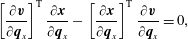
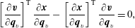
So the generalisation of equation (2.10) to a higher number of dimensions provides the following constraints:
 $$\begin{eqnarray}\displaystyle & \displaystyle \left[\frac{\unicode[STIX]{x2202}\boldsymbol{v}}{\unicode[STIX]{x2202}\boldsymbol{q}_{x}}\right]^{\text{T}}\frac{\unicode[STIX]{x2202}\boldsymbol{x}}{\unicode[STIX]{x2202}\boldsymbol{q}_{x}}-\left[\frac{\unicode[STIX]{x2202}\boldsymbol{x}}{\unicode[STIX]{x2202}\boldsymbol{q}_{x}}\right]^{\text{T}}\frac{\unicode[STIX]{x2202}\boldsymbol{v}}{\unicode[STIX]{x2202}\boldsymbol{q}_{x}}=0, & \displaystyle\end{eqnarray}$$
 $$\begin{eqnarray}\displaystyle & \displaystyle \left[\frac{\unicode[STIX]{x2202}\boldsymbol{v}}{\unicode[STIX]{x2202}\boldsymbol{q}_{v}}\right]^{\text{T}}\frac{\unicode[STIX]{x2202}\boldsymbol{x}}{\unicode[STIX]{x2202}\boldsymbol{q}_{v}}-\left[\frac{\unicode[STIX]{x2202}\boldsymbol{x}}{\unicode[STIX]{x2202}\boldsymbol{q}_{v}}\right]^{\text{T}}\frac{\unicode[STIX]{x2202}\boldsymbol{v}}{\unicode[STIX]{x2202}\boldsymbol{q}_{v}}=0, & \displaystyle\end{eqnarray}$$
 $$\begin{eqnarray}\displaystyle & \displaystyle \left[\frac{\unicode[STIX]{x2202}\boldsymbol{x}}{\unicode[STIX]{x2202}\boldsymbol{q}_{x}}\right]^{\text{T}}\frac{\unicode[STIX]{x2202}\boldsymbol{v}}{\unicode[STIX]{x2202}\boldsymbol{q}_{v}}-\left[\frac{\unicode[STIX]{x2202}\boldsymbol{v}}{\unicode[STIX]{x2202}\boldsymbol{q}_{x}}\right]^{\text{T}}\frac{\unicode[STIX]{x2202}\boldsymbol{x}}{\unicode[STIX]{x2202}\boldsymbol{q}_{v}}=\unicode[STIX]{x1D644}, & \displaystyle\end{eqnarray}$$
which can be again used to double check, a posteriori, the good behaviour of the code in the general case.
In the 2-D phase-space case considered here, the Hessian $\boldsymbol{H}$
is a
$\boldsymbol{H}$
is a $2\times 2\times 2$
tensor in which only 6 terms are independent if one just takes into account the symmetries in second derivatives, e.g.
$2\times 2\times 2$
tensor in which only 6 terms are independent if one just takes into account the symmetries in second derivatives, e.g. $\unicode[STIX]{x2202}^{2}x/(\unicode[STIX]{x2202}q_{x}\unicode[STIX]{x2202}q_{v})=\unicode[STIX]{x2202}^{2}x/(\unicode[STIX]{x2202}q_{v}\unicode[STIX]{x2202}q_{x})$
. In four- and six- dimensional phase space, the same symmetries imply that among its
$\unicode[STIX]{x2202}^{2}x/(\unicode[STIX]{x2202}q_{x}\unicode[STIX]{x2202}q_{v})=\unicode[STIX]{x2202}^{2}x/(\unicode[STIX]{x2202}q_{v}\unicode[STIX]{x2202}q_{x})$
. In four- and six- dimensional phase space, the same symmetries imply that among its $4\times 4\times 4=64$
and
$4\times 4\times 4=64$
and $6\times 6\times 6=$
216 elements, the Hessian includes 40 and 126 independent terms, respectively.
$6\times 6\times 6=$
216 elements, the Hessian includes 40 and 126 independent terms, respectively.
While exploiting the Hamiltonian nature of the system would allow us to carry less information, we chose for each element of metric to store the phase-space coordinates, the deformation tensor and the Hessian. The calculations above show that this ends up in carrying $2+4+6=12$
,
$2+4+6=12$
, $4+16+40=60$
and
$4+16+40=60$
and $6+36+126=168$
numbers for each element of metric in two-, four- and six-dimensional phase space, respectively. This might look a large number, particularly in four- and six-dimensional phase space, but one has to keep in mind the fact that elements of metric are much sparser than the grid used to compute the phase-space distribution function. For instance, a factor 3 in each direction of the spacing between elements of metric compared to the grid cell size implies that there is one element of metric for
$6+36+126=168$
numbers for each element of metric in two-, four- and six-dimensional phase space, respectively. This might look a large number, particularly in four- and six-dimensional phase space, but one has to keep in mind the fact that elements of metric are much sparser than the grid used to compute the phase-space distribution function. For instance, a factor 3 in each direction of the spacing between elements of metric compared to the grid cell size implies that there is one element of metric for $3^{6}=729$
grid sites. Another issue is the cost of applying the inverse mapping (2.7), but it can be reduced considerably by precomputing for each element of metric the matrixes
$3^{6}=729$
grid sites. Another issue is the cost of applying the inverse mapping (2.7), but it can be reduced considerably by precomputing for each element of metric the matrixes $\unicode[STIX]{x1D64F}_{m}^{-1}$
and
$\unicode[STIX]{x1D64F}_{m}^{-1}$
and $[\unicode[STIX]{x1D64F}_{m}^{-1}]^{\text{T}}\boldsymbol{H}_{m}\unicode[STIX]{x1D64F}_{m}^{-1}$
prior to any interpolation of the phase-space distribution function using the inverse mapping.
$[\unicode[STIX]{x1D64F}_{m}^{-1}]^{\text{T}}\boldsymbol{H}_{m}\unicode[STIX]{x1D64F}_{m}^{-1}$
prior to any interpolation of the phase-space distribution function using the inverse mapping.
2.2 Interpolation schemes
We use two interpolation schemes. Between two coarse steps, a period of time during which the phase-space distribution function is transported along motion using the same elements of metric at each time step, we use a simple interpolation of $f$
based on local fitting of a quadratic hypersurface. Then, during remapping, i.e. when new elements of metric are set,
$f$
based on local fitting of a quadratic hypersurface. Then, during remapping, i.e. when new elements of metric are set, $f$
is interpolated with a third-order spline in order to have a more accurate reconstruction of phase space. The advantage of using second-order interpolation during the transport phase is that generalisation to six-dimensional phase space is relatively cheap, since only 28 terms contribute in this case to such an interpolation. The loss of accuracy due to the relative roughness of the reconstruction, which is not even continuous, has little consequence for the dynamics because most of the information is recovered during the resampling phase. This will be tested and demonstrated in § 3. On the other hand, because our method does not allow for splitting,
$f$
is interpolated with a third-order spline in order to have a more accurate reconstruction of phase space. The advantage of using second-order interpolation during the transport phase is that generalisation to six-dimensional phase space is relatively cheap, since only 28 terms contribute in this case to such an interpolation. The loss of accuracy due to the relative roughness of the reconstruction, which is not even continuous, has little consequence for the dynamics because most of the information is recovered during the resampling phase. This will be tested and demonstrated in § 3. On the other hand, because our method does not allow for splitting, $4^{6}=4096$
terms contribute to each grid site when resampling
$4^{6}=4096$
terms contribute to each grid site when resampling $f$
in six dimensions with the third-order spline interpolation, if one assumes that this latter takes approximately 4 operations per grid site in one dimension. This rather costly step is thus approximately
$f$
in six dimensions with the third-order spline interpolation, if one assumes that this latter takes approximately 4 operations per grid site in one dimension. This rather costly step is thus approximately $4096/24\simeq 171$
times more expensive than what is expected when performing a full time step in the standard splitting algorithmFootnote
1
. It is however performed rarely, hence making the algorithm of potentially comparable cost to the standard semi-Lagrangian approach, with the advantage of being, in principle, less diffusive.
$4096/24\simeq 171$
times more expensive than what is expected when performing a full time step in the standard splitting algorithmFootnote
1
. It is however performed rarely, hence making the algorithm of potentially comparable cost to the standard semi-Lagrangian approach, with the advantage of being, in principle, less diffusive.
Now we provide the details for the second-order interpolation we use, followed by the standard third-order spline interpolation.
2.2.1 Second-order interpolation
The general procedure for second-order interpolation consists in understanding that a second-order hypersurface requires respectively 6, 15 and 28 points in 2-D, 4-D and 6-D phase space. What we have access to are the values $F(\boldsymbol{G})$
of the phase-space distribution function on a grid
$F(\boldsymbol{G})$
of the phase-space distribution function on a grid $\boldsymbol{G}$
, e.g. in two dimensions
$\boldsymbol{G}$
, e.g. in two dimensions $\boldsymbol{G}=(i,j)$
where
$\boldsymbol{G}=(i,j)$
where $i$
and
$i$
and $j$
are integers, corresponding to the following Lagrangian positions in phase space,
$j$
are integers, corresponding to the following Lagrangian positions in phase space,
 $$\begin{eqnarray}\displaystyle \boldsymbol{Q}_{G}=(i\unicode[STIX]{x0394}x+q_{x,mid},j\unicode[STIX]{x0394}v+q_{v,mid}), & & \displaystyle\end{eqnarray}$$
where $\unicode[STIX]{x0394}x$
and
$\unicode[STIX]{x0394}x$
and $\unicode[STIX]{x0394}v$
are the steps chosen for the grid (Eulerian or Lagrangian) that remain, in the current version of the code, fixed during runtime and
$\unicode[STIX]{x0394}v$
are the steps chosen for the grid (Eulerian or Lagrangian) that remain, in the current version of the code, fixed during runtime and $(q_{x,mid},q_{v,mid})$
corresponds to the middle of the Lagrangian computational domain. The bounds of the computational domain are then related to maximum values
$(q_{x,mid},q_{v,mid})$
corresponds to the middle of the Lagrangian computational domain. The bounds of the computational domain are then related to maximum values $n_{x}$
and
$n_{x}$
and $n_{v}$
of
$n_{v}$
of $|i|$
and
$|i|$
and $|j|$
.
$|j|$
.
This is the way we proceed in 2-D phase space: given a point $\boldsymbol{Q}=(q_{x},q_{v})$
in phase space, we first find the nearest grid point
$\boldsymbol{Q}=(q_{x},q_{v})$
in phase space, we first find the nearest grid point $(i_{n},j_{n})$
to it, then consider the cross composed of
$(i_{n},j_{n})$
to it, then consider the cross composed of $(i_{n}+1,j_{n})$
,
$(i_{n}+1,j_{n})$
, $(i_{n},j_{n}+1)$
,
$(i_{n},j_{n}+1)$
, $(i_{n}-1,j_{n})$
,
$(i_{n}-1,j_{n})$
, $(i_{n},j_{n}-1)$
and
$(i_{n},j_{n}-1)$
and $(i_{n},j_{n})$
on which the interpolation must coincide with
$(i_{n},j_{n})$
on which the interpolation must coincide with $F$
. The last point
$F$
. The last point $(i,j)$
needed is taken to be the one for which a square composed of 3 points of the cross and
$(i,j)$
needed is taken to be the one for which a square composed of 3 points of the cross and $(i,j)$
contains
$(i,j)$
contains $(q_{x},q_{v})$
(see figure 2). With this choice of the points of the grid for the interpolation, we have, at second order,
$(q_{x},q_{v})$
(see figure 2). With this choice of the points of the grid for the interpolation, we have, at second order,
 $$\begin{eqnarray}\displaystyle & & \displaystyle f(q_{x},q_{v})=F(i_{n},j_{n})(1-\text{d}q_{x}^{2}-\text{d}q_{v}^{2})\nonumber\\ \displaystyle & & \displaystyle \quad +\,{\textstyle \frac{1}{2}}F(i_{n}+1,j_{n})\,\text{d}q_{x}(1+\text{d}q_{x})+{\textstyle \frac{1}{2}}F(i_{n}-1,j_{n})\,\text{d}q_{x}(1-\text{d}q_{x})\nonumber\\ \displaystyle & & \displaystyle \quad +\,{\textstyle \frac{1}{2}}F(i_{n},j_{n}+1)\,\text{d}q_{v}(1+\text{d}q_{v})+{\textstyle \frac{1}{2}}F(i_{n}-1,j_{n})\,\text{d}q_{v}(1-\text{d}q_{v})\nonumber\\ \displaystyle & & \displaystyle \quad +\,[F(i_{c}+1,j_{c}+1)+F(i_{c},j_{c})-F(i_{c}+1,j_{c})-F(i_{c},j_{c}+1)]\,\text{d}q_{x}\,\text{d}q_{v},\qquad\end{eqnarray}$$
with
 $$\begin{eqnarray}\displaystyle & \displaystyle (i_{n},j_{n})=(\lfloor (q_{x}-q_{x,mid})/\unicode[STIX]{x0394}x\rceil ,\lfloor (q_{v}-q_{v,mid})/\unicode[STIX]{x0394}v\rceil ), & \displaystyle\end{eqnarray}$$
 $$\begin{eqnarray}\displaystyle & \displaystyle (i_{c},j_{c})=(\lfloor (q_{x}-q_{x,mid})/\unicode[STIX]{x0394}x\rfloor ,\lfloor (q_{v}-q_{v,mid})/\unicode[STIX]{x0394}v\rfloor ), & \displaystyle\end{eqnarray}$$
 $$\begin{eqnarray}\displaystyle & \displaystyle \text{d}q_{x}=(q_{x}-q_{x,mid})/\unicode[STIX]{x0394}x-i_{n}, & \displaystyle\end{eqnarray}$$
 $$\begin{eqnarray}\displaystyle & \displaystyle \text{d}q_{v}=(q_{v}-q_{v,mid})/\unicode[STIX]{x0394}v-j_{n}, & \displaystyle\end{eqnarray}$$
where $\lfloor \cdot \rceil$
and
$\lfloor \cdot \rceil$
and $\lfloor \cdot \rfloor$
are respectively the nearest integer and the integer part functions. Note obviously that when defining the edges of the computing domain, one makes sure that the interpolation is defined everywhere. In the present implementation,
$\lfloor \cdot \rfloor$
are respectively the nearest integer and the integer part functions. Note obviously that when defining the edges of the computing domain, one makes sure that the interpolation is defined everywhere. In the present implementation, $f$
is supposed to be different from zero on a compact domain in phase space. To avoid artificial enlarging of the computing domain during runtime due to diffusion and aliasing, the computing domain is restricted to a rectangular region containing all the points where
$f$
is supposed to be different from zero on a compact domain in phase space. To avoid artificial enlarging of the computing domain during runtime due to diffusion and aliasing, the computing domain is restricted to a rectangular region containing all the points where
 $$\begin{eqnarray}\displaystyle |f|>f_{th}, & & \displaystyle\end{eqnarray}$$
with $f_{th}$
a small number, typically
$f_{th}$
a small number, typically $f_{th}=10^{-6}$
. Note the absolute value in equation (2.23), because our algorithm does not enforce positivity of
$f_{th}=10^{-6}$
. Note the absolute value in equation (2.23), because our algorithm does not enforce positivity of $f$
and better total mass conservation is obtained by keeping the regions where
$f$
and better total mass conservation is obtained by keeping the regions where $f<0$
.
$f<0$
.
The generalisation of this second-order interpolation to higher number of dimensions is straightforward: the most difficult is to choose the grid points through which the hypersurface must pass. To achieve this, similarly as in two dimensions, we first find the nearest grid point $\boldsymbol{G}_{n}$
to
$\boldsymbol{G}_{n}$
to $\boldsymbol{Q}$
. Then take the collection of all segments centred on
$\boldsymbol{Q}$
. Then take the collection of all segments centred on $\boldsymbol{G}_{n}$
and composed of 3 points of the grid (the cross defined above in two dimensions): this provides us in total 9 and 13 points respectively in four and six dimensions. Then, project
$\boldsymbol{G}_{n}$
and composed of 3 points of the grid (the cross defined above in two dimensions): this provides us in total 9 and 13 points respectively in four and six dimensions. Then, project $\boldsymbol{Q}$
onto the planes defined by each pair of such segments and find the corresponding grid site in this plane such that the square composed of this grid site plus 3 contained in the 2 segments contains the projection of
$\boldsymbol{Q}$
onto the planes defined by each pair of such segments and find the corresponding grid site in this plane such that the square composed of this grid site plus 3 contained in the 2 segments contains the projection of $\boldsymbol{Q}$
and add it to our list of points defining the second-order hypersurface. There are 6 and 15 such points in four and six dimensions, respectively, and we thus end up using this procedure with respectively 15 and 28 points as needed to interpolate our hypersurface, with straightforward generalisation of equation (2.18) to perform the interpolation.
$\boldsymbol{Q}$
and add it to our list of points defining the second-order hypersurface. There are 6 and 15 such points in four and six dimensions, respectively, and we thus end up using this procedure with respectively 15 and 28 points as needed to interpolate our hypersurface, with straightforward generalisation of equation (2.18) to perform the interpolation.
Procedure employed to select the points of the grid used to perform second-order interpolation of the phase-space distribution function at position $\boldsymbol{Q}$
in
$\boldsymbol{Q}$
in $2D$
-dimensional phase space. One first finds the nearest grid point
$2D$
-dimensional phase space. One first finds the nearest grid point $\boldsymbol{G}_{n}$
to
$\boldsymbol{G}_{n}$
to $\boldsymbol{Q}$
,
$\boldsymbol{Q}$
, $\boldsymbol{G}_{n}=(i_{n},j_{n})$
for
$\boldsymbol{G}_{n}=(i_{n},j_{n})$
for $D=1$
, and select all the segments of the grid composed of 3 grid points and centred on
$D=1$
, and select all the segments of the grid composed of 3 grid points and centred on $\boldsymbol{G}_{n}$
: one obtains the red cross for one dimension. Then one selects, for each plane passing through a pair of such segments the four elements of the grid so that the square composed of these grid elements contains the projection of
$\boldsymbol{G}_{n}$
: one obtains the red cross for one dimension. Then one selects, for each plane passing through a pair of such segments the four elements of the grid so that the square composed of these grid elements contains the projection of $\boldsymbol{Q}$
: one of them,
$\boldsymbol{Q}$
: one of them, $(i_{c}+1,j_{c}+1)$
on the figure, provides one additional point for the interpolation.
$(i_{c}+1,j_{c}+1)$
on the figure, provides one additional point for the interpolation.

2.2.2 Standard third-order spline
The third-order interpolation we use employs standard cubic B-splines as very clearly described in e.g. Crouseilles, Latu & Sonnendrücker (Reference Crouseilles, Latu and Sonnendrücker2009), so we do not provide the detail here, except the edge conditions, which are
 $$\begin{eqnarray}\displaystyle f(q_{x},q_{v})=0,\quad \frac{\unicode[STIX]{x2202}f}{\unicode[STIX]{x2202}q_{x}}=0,\quad |q_{x}|=q_{x,mid}+n_{x}\unicode[STIX]{x0394}x, & & \displaystyle\end{eqnarray}$$
 $$\begin{eqnarray}\displaystyle f(q_{x},q_{v})=0,\quad \frac{\unicode[STIX]{x2202}f}{\unicode[STIX]{x2202}q_{v}}=0,\quad |q_{v}|=q_{v,mid}+n_{v}\unicode[STIX]{x0394}v, & & \displaystyle\end{eqnarray}$$
and this can be trivially generalised to four- or six-dimensional phase space.
2.3 Tracing back the characteristics in Lagrangian space: percolation algorithm
To determine the value of $f(\boldsymbol{P},t)$
, we have to trace the trajectory of a test particle coinciding with
$f(\boldsymbol{P},t)$
, we have to trace the trajectory of a test particle coinciding with $\boldsymbol{P}$
back to its Lagrangian, initial position
$\boldsymbol{P}$
back to its Lagrangian, initial position $\boldsymbol{Q}$
(the position at time of remapping, in general). To do this, we need to find the closest element of metric to this test particle and use equation (2.7) to compute
$\boldsymbol{Q}$
(the position at time of remapping, in general). To do this, we need to find the closest element of metric to this test particle and use equation (2.7) to compute $\boldsymbol{Q}$
. However, the closest element of metric, from the dynamical point of view, has to be found in Lagrangian space, which complicates the procedure. Furthermore, two close test particles might end up associated with different elements of metric that will propose slightly different mappings, implying that function
$\boldsymbol{Q}$
. However, the closest element of metric, from the dynamical point of view, has to be found in Lagrangian space, which complicates the procedure. Furthermore, two close test particles might end up associated with different elements of metric that will propose slightly different mappings, implying that function $\boldsymbol{Q}(\boldsymbol{P})$
is discontinuous if no supplementary treatment is performed. While this is not too problematic during the transport phase, it can have dramatic consequences on the long term during the remapping step which requires a high level of precision when interpolating the phase-space distribution function with third-order splines. Hence, each time a full remapping of
$\boldsymbol{Q}(\boldsymbol{P})$
is discontinuous if no supplementary treatment is performed. While this is not too problematic during the transport phase, it can have dramatic consequences on the long term during the remapping step which requires a high level of precision when interpolating the phase-space distribution function with third-order splines. Hence, each time a full remapping of $f$
is performed, one needs to find not one but several elements of metric in the neighbourhood of a test particle to be able to interpolate between the proposed Lagrangian positions provided by each of these metric elements so that function
$f$
is performed, one needs to find not one but several elements of metric in the neighbourhood of a test particle to be able to interpolate between the proposed Lagrangian positions provided by each of these metric elements so that function $\boldsymbol{Q}(\boldsymbol{P})$
stays smooth: this is the most complex part of the algorithm, because enforcing full continuity of the interpolation is actually not trivial since it has to be performed in Lagrangian space. The percolation algorithm however allows us to define in an unambiguous way regions of influence of each element of metric which in turn will allow us to make function
$\boldsymbol{Q}(\boldsymbol{P})$
stays smooth: this is the most complex part of the algorithm, because enforcing full continuity of the interpolation is actually not trivial since it has to be performed in Lagrangian space. The percolation algorithm however allows us to define in an unambiguous way regions of influence of each element of metric which in turn will allow us to make function $\boldsymbol{Q}(\boldsymbol{P})$
smooth.
$\boldsymbol{Q}(\boldsymbol{P})$
smooth.
We assume that elements of metric are initially set on a Lagrangian grid covering the computing domain, $\boldsymbol{M}=(i_{m},j_{m})$
, corresponding to Lagrangian positions
$\boldsymbol{M}=(i_{m},j_{m})$
, corresponding to Lagrangian positions
 $$\begin{eqnarray}\displaystyle \boldsymbol{Q}_{m}(i_{m},j_{m})=(\unicode[STIX]{x0394}x_{m}i_{m}+q_{x,mid},\unicode[STIX]{x0394}v_{m}\,j_{m}+q_{v,mid}), & & \displaystyle\end{eqnarray}$$
with
 $$\begin{eqnarray}\displaystyle \unicode[STIX]{x0394}x_{m}\gtrsim \unicode[STIX]{x0394}x,\quad \unicode[STIX]{x0394}v_{m}\gtrsim \unicode[STIX]{x0394}v. & & \displaystyle\end{eqnarray}$$
The actual computing domain changes subsequently with time. To estimate it at each time step we use the positions of the metric elements and we define a rectangle with lower left and upper right corners respectively given by $[\text{min}_{i_{m},j_{m}}(x_{m}),\text{min}_{i_{m},j_{m}}(v_{m})]$
and
$[\text{min}_{i_{m},j_{m}}(x_{m}),\text{min}_{i_{m},j_{m}}(v_{m})]$
and $[\text{max}_{i_{m},j_{m}}(x_{m}),\text{max}_{i_{m},j_{m}}(v_{m})]$
. This means that the element of metric coverage should be wide enough to avoid missing regions where
$[\text{max}_{i_{m},j_{m}}(x_{m}),\text{max}_{i_{m},j_{m}}(v_{m})]$
. This means that the element of metric coverage should be wide enough to avoid missing regions where $f$
should be not equal to zero. We therefore allow for an extra layer of metric elements on all the sides of the Lagrangian computing domain. Note thus that the calculation of the computing domain is far from optimal, which can have dramatic consequences for the cost of the algorithm in six dimensions. In order to fix this problem, one would need to define a more complex shape-dependent computational domain by e.g. constructing a k-d tree, i.e. a spatial decomposition of phase space with nested cubes. Such a k-d tree could also constitute the basis for an adaptive mesh refinement algorithm following in an optimal way not only the computational domain, but also all the details of the phase-space distribution function when needed. However such a sophistication is not needed in our 2-D implementation so we stick to the rectangular computing domain for now.
$f$
should be not equal to zero. We therefore allow for an extra layer of metric elements on all the sides of the Lagrangian computing domain. Note thus that the calculation of the computing domain is far from optimal, which can have dramatic consequences for the cost of the algorithm in six dimensions. In order to fix this problem, one would need to define a more complex shape-dependent computational domain by e.g. constructing a k-d tree, i.e. a spatial decomposition of phase space with nested cubes. Such a k-d tree could also constitute the basis for an adaptive mesh refinement algorithm following in an optimal way not only the computational domain, but also all the details of the phase-space distribution function when needed. However such a sophistication is not needed in our 2-D implementation so we stick to the rectangular computing domain for now.
2.3.1 Percolation
To compute the region of influence of each element of metric $(i_{m},j_{m})$
with coordinates
$(i_{m},j_{m})$
with coordinates $(x_{m},v_{m})$
, we percolate around it on the Eulerian computational grid starting from its nearest grid point
$(x_{m},v_{m})$
, we percolate around it on the Eulerian computational grid starting from its nearest grid point
 $$\begin{eqnarray}\displaystyle (i,j)=(\lfloor (x_{m}-x_{mid})/\unicode[STIX]{x0394}x\rceil ,\lfloor (v_{m}-v_{mid})/\unicode[STIX]{x0394}v\rceil ), & & \displaystyle\end{eqnarray}$$
with $(x_{mid},v_{mid})$
being the time-dependent position of the middle of the Eulerian computational domain. The initial Lagrangian position
$(x_{mid},v_{mid})$
being the time-dependent position of the middle of the Eulerian computational domain. The initial Lagrangian position $\boldsymbol{Q}(i,j,i_{m},j_{m})$
of this point is estimated with equation (2.7) using the element of metric we started from as a reference. Note that another neighbouring element of metric
$\boldsymbol{Q}(i,j,i_{m},j_{m})$
of this point is estimated with equation (2.7) using the element of metric we started from as a reference. Note that another neighbouring element of metric $(i_{m}^{\prime },j_{m}^{\prime })$
would propose a slightly different value for the initial position of the test particle associated with Eulerian grid site
$(i_{m}^{\prime },j_{m}^{\prime })$
would propose a slightly different value for the initial position of the test particle associated with Eulerian grid site $(i,j)$
, hence the dependence on
$(i,j)$
, hence the dependence on $(i_{m},j_{m})$
of
$(i_{m},j_{m})$
of $\boldsymbol{Q}$
. Then one defines the function
$\boldsymbol{Q}$
. Then one defines the function
 $$\begin{eqnarray}\displaystyle \unicode[STIX]{x1D6FF}\boldsymbol{Q}(i,j,i_{m},j_{m}) & \equiv & \displaystyle [\unicode[STIX]{x1D6FF}q_{x}(i,j,i_{m},j_{m}),\unicode[STIX]{x1D6FF}q_{v}(i,j,i_{m},j_{m})]\end{eqnarray}$$
 $$\begin{eqnarray}\displaystyle & \equiv & \displaystyle \boldsymbol{Q}(i,j,i_{m},j_{m})-\boldsymbol{Q}_{m}(i_{m},j_{m}),\end{eqnarray}$$
where $\boldsymbol{Q}_{m}(i_{m},j_{m})$
is the Lagrangian position of the element of metric, to find out which neighbours
$\boldsymbol{Q}_{m}(i_{m},j_{m})$
is the Lagrangian position of the element of metric, to find out which neighbours $(i_{m}^{\prime },j_{m}^{\prime })$
of the element of metric are susceptible to be closer to the true initial
$(i_{m}^{\prime },j_{m}^{\prime })$
of the element of metric are susceptible to be closer to the true initial $\boldsymbol{Q}(i,j)$
in Lagrangian space. Because the calculation of
$\boldsymbol{Q}(i,j)$
in Lagrangian space. Because the calculation of $\boldsymbol{Q}(i,j)$
is not exact we need to introduce the concept of uncertainty. Considering all the neighbours of the current element of metric under consideration
$\boldsymbol{Q}(i,j)$
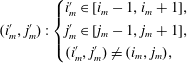
is not exact we need to introduce the concept of uncertainty. Considering all the neighbours of the current element of metric under consideration
 $$\begin{eqnarray}\displaystyle (i_{m}^{\prime },j_{m}^{\prime }):\left\{\begin{array}{@{}l@{}}i_{m}^{\prime }\in [i_{m}-1,i_{m}+1],\\ j_{m}^{\prime }\in [j_{m}-1,j_{m}+1],\\ (i_{m}^{\prime },j_{m}^{\prime })\neq (i_{m},j_{m}),\end{array}\right. & & \displaystyle\end{eqnarray}$$
we are able to chose the one which proposes the smallest value of
 $$\begin{eqnarray}\displaystyle d[\unicode[STIX]{x1D6FF}\boldsymbol{Q}(i,j,i_{m},j_{m})]\equiv \sqrt{(\unicode[STIX]{x1D6FF}q_{x}/\unicode[STIX]{x0394}x)^{2}+(\unicode[STIX]{x1D6FF}q_{v}/\unicode[STIX]{x0394}v)^{2}}, & & \displaystyle\end{eqnarray}$$
where the dependence on $(i,j,i_{m},j_{m})$
of
$(i,j,i_{m},j_{m})$
of $\unicode[STIX]{x1D6FF}q_{x}$
and
$\unicode[STIX]{x1D6FF}q_{x}$
and $\unicode[STIX]{x1D6FF}q_{v}$
has been made implicit. If there is a candidate element of metric
$\unicode[STIX]{x1D6FF}q_{v}$
has been made implicit. If there is a candidate element of metric $(i_{m}^{\prime },j_{m}^{\prime })$
closer than
$(i_{m}^{\prime },j_{m}^{\prime })$
closer than $(i_{m},j_{m})$
to the Eulerian grid element
$(i_{m},j_{m})$
to the Eulerian grid element $(i,j)$
using this Lagrangian distance, the percolation process is stopped. Otherwise, one continues (bond) percolation i.e. proceeds with neighbouring grid sites
$(i,j)$
using this Lagrangian distance, the percolation process is stopped. Otherwise, one continues (bond) percolation i.e. proceeds with neighbouring grid sites $(i+1,j)$
,
$(i+1,j)$
, $(i-1,j)$
,
$(i-1,j)$
, $(i,j+1)$
,
$(i,j+1)$
, $(i,j-1)$
unless they have been already processed.
$(i,j-1)$
unless they have been already processed.
Note that the percolation procedure just defined above is not always free of aliasing: it can be successful only if the separation between elements of metric is sufficiently large compared to the grid element size and if their zone of influence is not too distorted. Testing the validity of the percolation process is relatively simple, by checking if some points inside the computing domain have been left unexplored. If it is the case, percolation is performed again locally until all the unexplored points are processed, which induces a small additional cost in the algorithm.
To speed up the process, which is not really relevant here in 2-D phase space but crucial in a higher number of dimensions, we reduce the range of investigation of values of $i_{m}^{\prime }$
to
$i_{m}^{\prime }$
to $[i_{inf},i_{sup}]$
where
$[i_{inf},i_{sup}]$
where
 $$\begin{eqnarray}\displaystyle & \displaystyle \unicode[STIX]{x1D6FF}q_{x}<-\unicode[STIX]{x1D6FC}\unicode[STIX]{x0394}x_{m}:i_{inf}=-1,i_{sup}=0, & \displaystyle\end{eqnarray}$$
 $$\begin{eqnarray}\displaystyle & \displaystyle -\unicode[STIX]{x1D6FC}\unicode[STIX]{x0394}x_{m}\leqslant \unicode[STIX]{x1D6FF}q_{x}<\unicode[STIX]{x1D6FC}\unicode[STIX]{x0394}x_{m}:i_{inf}=0,i_{sup}=0, & \displaystyle\end{eqnarray}$$
 $$\begin{eqnarray}\displaystyle & \displaystyle \unicode[STIX]{x1D6FC}\unicode[STIX]{x0394}x_{m}\leqslant \unicode[STIX]{x1D6FF}q_{x}:i_{inf}=0,i_{sup}=1, & \displaystyle\end{eqnarray}$$
with the dependence on $(i,j,i_{m},j_{m})$
of
$(i,j,i_{m},j_{m})$
of $\unicode[STIX]{x1D6FF}q_{x}$
still implicit and
$\unicode[STIX]{x1D6FF}q_{x}$
still implicit and $\unicode[STIX]{x1D6FC}$
is a parameter close to
$\unicode[STIX]{x1D6FC}$
is a parameter close to $1/2$
. Similar conditions are set to define an interval
$1/2$
. Similar conditions are set to define an interval $[j_{inf},j_{sup}]$
. The parameter
$[j_{inf},j_{sup}]$
. The parameter $\unicode[STIX]{x1D6FC}$
is introduced to take into account the uncertainty
$\unicode[STIX]{x1D6FC}$
is introduced to take into account the uncertainty $\boldsymbol{E}_{map}=(E_{x},E_{v})$
on the remapping (2.7). This is illustrated by figure 3. However, even though we can actually estimate
$\boldsymbol{E}_{map}=(E_{x},E_{v})$
on the remapping (2.7). This is illustrated by figure 3. However, even though we can actually estimate $\boldsymbol{E}_{map}$
as described below in § 2.3.3, we do not use it to calculate
$\boldsymbol{E}_{map}$
as described below in § 2.3.3, we do not use it to calculate $\unicode[STIX]{x1D6FC}$
which is fixed from the beginning. Indeed, our implementation favours performance over perfect accuracy, to make a future extension to 6-D phase space possible: while it is better to find in Lagrangian space the actual nearest element of metric to a test particle, this is not a must and the algorithm can still work without it, at the cost of some loss of accuracy on the long run.
$\unicode[STIX]{x1D6FC}$
which is fixed from the beginning. Indeed, our implementation favours performance over perfect accuracy, to make a future extension to 6-D phase space possible: while it is better to find in Lagrangian space the actual nearest element of metric to a test particle, this is not a must and the algorithm can still work without it, at the cost of some loss of accuracy on the long run.
Scheme determining the range of investigation of neighbouring elements of metric during the percolation process in Lagrangian space. We consider a pixel $\boldsymbol{P}$
in Eulerian space that we know to be already close to an element of metric
$\boldsymbol{P}$
in Eulerian space that we know to be already close to an element of metric $(i_{m},j_{m})$
because it is a direct neighbour of a pixel known to be in the region of influence of
$(i_{m},j_{m})$
because it is a direct neighbour of a pixel known to be in the region of influence of $(i_{m},j_{m})$
. We remap it to its Lagrangian counterpart
$(i_{m},j_{m})$
. We remap it to its Lagrangian counterpart $\boldsymbol{Q}$
using the element of metric
$\boldsymbol{Q}$
using the element of metric $(i_{m},j_{m})$
. Then we aim to find the closest element of metric to it. To do so and speed up the process, four cases are considered, to take into account the small errors on
$(i_{m},j_{m})$
. Then we aim to find the closest element of metric to it. To do so and speed up the process, four cases are considered, to take into account the small errors on $\boldsymbol{Q}$
(in particular the fact that the reconstructed
$\boldsymbol{Q}$
(in particular the fact that the reconstructed $\boldsymbol{Q}$
depends on the element of metric under consideration, see figure 1), that we write
$\boldsymbol{Q}$
depends on the element of metric under consideration, see figure 1), that we write $\boldsymbol{E}_{map}=(E_{x},E_{v})$
. In case 4,
$\boldsymbol{E}_{map}=(E_{x},E_{v})$
. In case 4, $\boldsymbol{Q}$
is close enough to the element of metric: we do not need to investigate any neighbour and decide it to belong to the region of influence of
$\boldsymbol{Q}$
is close enough to the element of metric: we do not need to investigate any neighbour and decide it to belong to the region of influence of $(i_{m},j_{m})$
. In cases 2 and 3, we need only to investigate another element of metric, e.g.
$(i_{m},j_{m})$
. In cases 2 and 3, we need only to investigate another element of metric, e.g. $(i_{m},j_{m}+1)$
in the upper part of the figure to decide if it closer to its own estimate of
$(i_{m},j_{m}+1)$
in the upper part of the figure to decide if it closer to its own estimate of $\boldsymbol{Q}$
using the distance defined in equation (2.32). Finally case 1 is the most costly since we have to investigate three neighbouring element of metric, but it is seldom considered.
$\boldsymbol{Q}$
using the distance defined in equation (2.32). Finally case 1 is the most costly since we have to investigate three neighbouring element of metric, but it is seldom considered.

To illustrate the result of the percolation process, figure 4 displays, at $t=25$
, the region of influence of each element of metric at the end of a cycle (i.e. just before resampling with new elements of metric) for the simulation II with Gaussian initial condition described in § 3.
$t=25$
, the region of influence of each element of metric at the end of a cycle (i.e. just before resampling with new elements of metric) for the simulation II with Gaussian initial condition described in § 3.
Gaussian run and percolation. (a) The phase-space distribution function is shown at $t=25$
for a simulation with Gaussian initial conditions and parameters corresponding to item II of table 1 in § 3. (b) The corresponding Lagrangian zone of influence of each element of metric obtained from the percolation process is drawn at the end of a cycle (just before full resampling with new metric elements). To visualise the results more clearly, a random colour has been associated with each element of metric.
$t=25$
for a simulation with Gaussian initial conditions and parameters corresponding to item II of table 1 in § 3. (b) The corresponding Lagrangian zone of influence of each element of metric obtained from the percolation process is drawn at the end of a cycle (just before full resampling with new metric elements). To visualise the results more clearly, a random colour has been associated with each element of metric.

2.3.2 Interpolation of the Lagrangian position of a test particle
We now explain how the Lagrangian position of a test particle can be calculated in a smooth way with proper interpolation in Lagrangian space between predicates given by each of neighbouring elements of metric. We define the following mapping function $\boldsymbol{Q}_{r}(\boldsymbol{P})$
from Eulerian to Lagrangian space
$\boldsymbol{Q}_{r}(\boldsymbol{P})$
from Eulerian to Lagrangian space
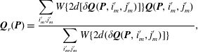 $$\begin{eqnarray}\displaystyle \boldsymbol{Q}_{r}(\boldsymbol{P})\equiv \frac{\displaystyle \mathop{\sum }_{i_{m}^{\prime },j_{m}^{\prime }}W\{2d[\unicode[STIX]{x1D6FF}\boldsymbol{Q}(\boldsymbol{P},i_{m}^{\prime },j_{m}^{\prime })]\}\boldsymbol{Q}(\boldsymbol{P},i_{m}^{\prime },j_{m}^{\prime })}{\displaystyle \mathop{\sum }_{i_{m}^{\prime },j_{m}^{\prime }}W\{2d(\unicode[STIX]{x1D6FF}\boldsymbol{Q}(\boldsymbol{P},i_{m}^{\prime },j_{m}^{\prime })]\}}, & & \displaystyle\end{eqnarray}$$
where function $\boldsymbol{Q}(\boldsymbol{P},i_{m},j_{m})$
is the obvious extension to the continuum of its discrete counterpart
$\boldsymbol{Q}(\boldsymbol{P},i_{m},j_{m})$
is the obvious extension to the continuum of its discrete counterpart $\boldsymbol{Q}(i,j,i_{m},j_{m})$
defined previously, likewise for
$\boldsymbol{Q}(i,j,i_{m},j_{m})$
defined previously, likewise for $\unicode[STIX]{x1D6FF}\boldsymbol{Q}(\boldsymbol{P},i_{m},j_{m})$
, and
$\unicode[STIX]{x1D6FF}\boldsymbol{Q}(\boldsymbol{P},i_{m},j_{m})$
, and $W(x)$
is a smooth isotropic kernel function compactly supported. Clearly, function
$W(x)$
is a smooth isotropic kernel function compactly supported. Clearly, function $\boldsymbol{Q}_{r}(\boldsymbol{P})$
as defined above is at least continuous. Our choice for
$\boldsymbol{Q}_{r}(\boldsymbol{P})$
as defined above is at least continuous. Our choice for $W(x)$
is the spline of Monaghan (Reference Monaghan1992):
$W(x)$
is the spline of Monaghan (Reference Monaghan1992):
 $$\begin{eqnarray}\displaystyle W(x)\equiv \left\{\begin{array}{@{}ll@{}}\displaystyle 1-{\textstyle \frac{3}{2}}x^{2}+{\textstyle \frac{3}{4}}x^{3}, & x\leqslant 1,\\ \displaystyle {\textstyle \frac{1}{4}}(2-x)^{3}, & 1<x\leqslant 2,\\ \displaystyle 0, & x>2,\end{array}\right. & & \displaystyle\end{eqnarray}$$
which preserves the second-order nature of the Taylor expansion around each metric element position. Our choice of $W(x)$
allows us to restrict the range of investigation of values of
$W(x)$
allows us to restrict the range of investigation of values of $i_{m}^{\prime }$
and
$i_{m}^{\prime }$
and $j_{m}^{\prime }$
to the respective intervals
$j_{m}^{\prime }$
to the respective intervals $[i_{m}-1,i_{m}+1]$
and
$[i_{m}-1,i_{m}+1]$
and $[j_{m}-1,j_{m}+1]$
where
$[j_{m}-1,j_{m}+1]$
where $(i_{m},j_{m})$
corresponds to the closest element of metric to point
$(i_{m},j_{m})$
corresponds to the closest element of metric to point $\boldsymbol{P}$
as computed in the previous paragraph, § 2.3.1, for sites
$\boldsymbol{P}$
as computed in the previous paragraph, § 2.3.1, for sites $(i,j)$
of a gridFootnote
2
. Here, we indeed only need to consider points
$(i,j)$
of a gridFootnote
2
. Here, we indeed only need to consider points $\boldsymbol{P}=(\unicode[STIX]{x0394}xi+x_{mid},\unicode[STIX]{x0394}vj+v_{mid})$
associated with such an Eulerian grid. To reduce furthermore the number of elements of metric investigated to perform the interpolation (2.36) while still taking into account small variations related to the previously discussed uncertainty
$\boldsymbol{P}=(\unicode[STIX]{x0394}xi+x_{mid},\unicode[STIX]{x0394}vj+v_{mid})$
associated with such an Eulerian grid. To reduce furthermore the number of elements of metric investigated to perform the interpolation (2.36) while still taking into account small variations related to the previously discussed uncertainty $\boldsymbol{E}_{map}$
on the calculation of
$\boldsymbol{E}_{map}$
on the calculation of $\boldsymbol{Q}$
, we restrict the search to the intervals
$\boldsymbol{Q}$
, we restrict the search to the intervals $[i_{min},i_{max}]$
and
$[i_{min},i_{max}]$
and $[j_{min},j_{max}]$
defined as follows, with the same notations as in equations (2.33), (2.34) and (2.35):
$[j_{min},j_{max}]$
defined as follows, with the same notations as in equations (2.33), (2.34) and (2.35):
 $$\begin{eqnarray}\displaystyle & \displaystyle \unicode[STIX]{x1D6FF}q_{x}<-\unicode[STIX]{x1D6FD}\unicode[STIX]{x0394}x_{m}:i_{min}=-1,i_{max}=0, & \displaystyle\end{eqnarray}$$
 $$\begin{eqnarray}\displaystyle & \displaystyle -\unicode[STIX]{x1D6FD}\unicode[STIX]{x0394}x_{m}\leqslant \unicode[STIX]{x1D6FF}q_{x}<\unicode[STIX]{x1D6FD}\unicode[STIX]{x0394}x_{m}:i_{min}=-1,i_{max}=1, & \displaystyle\end{eqnarray}$$
 $$\begin{eqnarray}\displaystyle & \displaystyle \unicode[STIX]{x1D6FD}\unicode[STIX]{x0394}x_{m}\leqslant \unicode[STIX]{x1D6FF}q_{x}:i_{min}=0,i_{max}=1, & \displaystyle\end{eqnarray}$$
where $\unicode[STIX]{x1D6FD}$
is a small parameter accounting for the error
$\unicode[STIX]{x1D6FD}$
is a small parameter accounting for the error $\boldsymbol{E}_{map}$
, similarly for
$\boldsymbol{E}_{map}$
, similarly for $j_{min}$
and
$j_{min}$
and $j_{max}$
, with the additional constraint
$j_{max}$
, with the additional constraint $i_{m}^{\prime }\,j_{m}^{\prime }=0$
if
$i_{m}^{\prime }\,j_{m}^{\prime }=0$
if $i_{min}i_{max}=-1$
or
$i_{min}i_{max}=-1$
or $j_{min}\,j_{max}=-1$
to gain even more time.
$j_{min}\,j_{max}=-1$
to gain even more time.
Again, similarly as stated at the end of § 2.3.1, the above algorithm is not guaranteed to provide a smooth interpolation if the error on the remapping associated with the metric elements becomes larger than some threshold. However, this should have little consequence for the algorithm accuracy and the gain of speed in high-dimensional phase space is considerable with such a procedure. Indeed, if $\boldsymbol{E}_{map}$
becomes too large, the loss of accuracy on the characteristics themselves is much more dramatic than small discontinuities introduced on their interpolation.
$\boldsymbol{E}_{map}$
becomes too large, the loss of accuracy on the characteristics themselves is much more dramatic than small discontinuities introduced on their interpolation.
2.3.3 Estimates of errors on the Lagrangian position and choice of the margin parameters $\unicode[STIX]{x1D6FC}$
and
$\unicode[STIX]{x1D6FD}$
$\unicode[STIX]{x1D6FC}$
and
$\unicode[STIX]{x1D6FD}$


In the two subsections above, we defined two parameters $\unicode[STIX]{x1D6FC}$
and
$\unicode[STIX]{x1D6FC}$
and $\unicode[STIX]{x1D6FD}$
but did not provide any numerical values. In principle these parameters could be user defined, but we choose to fix them:
$\unicode[STIX]{x1D6FD}$
but did not provide any numerical values. In principle these parameters could be user defined, but we choose to fix them:
 $$\begin{eqnarray}\displaystyle & \displaystyle \unicode[STIX]{x1D6FC}={\textstyle \frac{\sqrt{3}}{4}}\simeq 0.43, & \displaystyle\end{eqnarray}$$
 $$\begin{eqnarray}\displaystyle & \displaystyle \unicode[STIX]{x1D6FD}={\textstyle \frac{1}{2}}\left(1-{\textstyle \frac{\sqrt{3}}{2}}\right)\simeq 0.067. & \displaystyle\end{eqnarray}$$
The idea behind this choice is the following. Firstly, according to figure 5, since we do not want to consider any diagonal element of metric if $i_{min}i_{max}=-1$
or
$i_{min}i_{max}=-1$
or $j_{min}j_{max}=1$
, we must have for full consistency,
$j_{min}j_{max}=1$
, we must have for full consistency,
 $$\begin{eqnarray}\displaystyle \unicode[STIX]{x1D6FD}\leqslant 1-{\textstyle \frac{\sqrt{3}}{2}}\simeq 0.13. & & \displaystyle\end{eqnarray}$$
Because there is some error on the reconstructed value of $\boldsymbol{Q}$
, we take half this value, assuming that
$\boldsymbol{Q}$
, we take half this value, assuming that
 $$\begin{eqnarray}\displaystyle E_{x}/\unicode[STIX]{x0394}x_{m},E_{y}/\unicode[STIX]{x0394}v_{m}\leqslant E_{max}\equiv {\textstyle \frac{1}{2}}\left(1-{\textstyle \frac{\sqrt{3}}{2}}\right)\simeq 0.067. & & \displaystyle\end{eqnarray}$$
Hence $\unicode[STIX]{x1D6FC}=1/2-E_{max}$
is given by equation (2.41) to take into account this upper bound for the errors. With this setting, the algorithm is fully consistent only if the uncertainty on the remapped trajectories remains small enough, but even if
$\unicode[STIX]{x1D6FC}=1/2-E_{max}$
is given by equation (2.41) to take into account this upper bound for the errors. With this setting, the algorithm is fully consistent only if the uncertainty on the remapped trajectories remains small enough, but even if $E_{x}/\unicode[STIX]{x0394}x_{m}$
or
$E_{x}/\unicode[STIX]{x0394}x_{m}$
or $E_{v}/\unicode[STIX]{x0394}v_{m}$
are larger than
$E_{v}/\unicode[STIX]{x0394}v_{m}$
are larger than $E_{max}$
, it still works. It is simply the case that function
$E_{max}$
, it still works. It is simply the case that function $\boldsymbol{Q}_{r}(\boldsymbol{P})$
is not guaranteed to be completely smooth anymore.
$\boldsymbol{Q}_{r}(\boldsymbol{P})$
is not guaranteed to be completely smooth anymore.
Note that in our algorithm, a global error $E_{map}=\sqrt{(E_{x}/\unicode[STIX]{x0394}x_{m})^{2}+(E_{v}/\unicode[STIX]{x0394}v_{m})^{2}}$
is estimated during the percolation process by comparing the value of
$E_{map}=\sqrt{(E_{x}/\unicode[STIX]{x0394}x_{m})^{2}+(E_{v}/\unicode[STIX]{x0394}v_{m})^{2}}$
is estimated during the percolation process by comparing the value of $\boldsymbol{Q}$
proposed by a neighbouring element of metric to the value of
$\boldsymbol{Q}$
proposed by a neighbouring element of metric to the value of $\boldsymbol{Q}$
proposed by the element of metric under consideration using the Lagrangian distance
$\boldsymbol{Q}$
proposed by the element of metric under consideration using the Lagrangian distance $d$
defined in equation (2.32). Such an error can in principle be used to force global remapping if
$d$
defined in equation (2.32). Such an error can in principle be used to force global remapping if $E_{map}$
exceeds some threshold, for instance
$E_{map}$
exceeds some threshold, for instance $E_{max}$
to preserve full smoothness of function
$E_{max}$
to preserve full smoothness of function $\boldsymbol{Q}_{r}(\boldsymbol{P})$
. While this is an option in our code, we do not use it for the tests performed in § 3. Indeed, we found difficult to find some reliable criterion on
$\boldsymbol{Q}_{r}(\boldsymbol{P})$
. While this is an option in our code, we do not use it for the tests performed in § 3. Indeed, we found difficult to find some reliable criterion on $E_{map}$
and preferred to keep the number
$E_{map}$
and preferred to keep the number $n_{s}$
of time steps between full resampling fixed and see how the results depend on the choice of
$n_{s}$
of time steps between full resampling fixed and see how the results depend on the choice of $n_{s}$
, being aware of the fact that this is potentially suboptimal. Note also that
$n_{s}$
, being aware of the fact that this is potentially suboptimal. Note also that $E_{x}$
and
$E_{x}$
and $E_{v}$
could be estimated as the residuals from the third-order description of the local metric elements, but this is very costly in highly dimensional phase space.
$E_{v}$
could be estimated as the residuals from the third-order description of the local metric elements, but this is very costly in highly dimensional phase space.
Scheme determining the number of neighbouring elements of metric to consider for the interpolation (2.36) used to reconstruct the Lagrangian coordinate $\boldsymbol{Q}$
of a test particle
$\boldsymbol{Q}$
of a test particle $\boldsymbol{P}$
in the region of influence of metric element
$\boldsymbol{P}$
in the region of influence of metric element $(i_{m},j_{m})$
. This figure also justifies equation (2.43). Each element of metric has an ellipsoid region of influence (ocher ellipse) for computing the weights in equation (2.36). Outside this area, the element of metric does not contribute. Therefore, in the absence of uncertainty on the reconstruction of the Lagrangian coordinate, one can safely define 4 kinds of regions, as shown on the figure, with
$(i_{m},j_{m})$
. This figure also justifies equation (2.43). Each element of metric has an ellipsoid region of influence (ocher ellipse) for computing the weights in equation (2.36). Outside this area, the element of metric does not contribute. Therefore, in the absence of uncertainty on the reconstruction of the Lagrangian coordinate, one can safely define 4 kinds of regions, as shown on the figure, with $h_{x}=(1-\sqrt{3}/2)\unicode[STIX]{x0394}x_{m}$
and
$h_{x}=(1-\sqrt{3}/2)\unicode[STIX]{x0394}x_{m}$
and $h_{v}=(1-\sqrt{3}/2)\unicode[STIX]{x0394}v_{m}$
, steaming from the ellipse equations
$h_{v}=(1-\sqrt{3}/2)\unicode[STIX]{x0394}v_{m}$
, steaming from the ellipse equations $(1-h_{x}/\unicode[STIX]{x0394}x_{m})^{2}+1/4=1$
and
$(1-h_{x}/\unicode[STIX]{x0394}x_{m})^{2}+1/4=1$
and $1/4+(1-h_{v}/\unicode[STIX]{x0394}v_{m})^{2}=1$
. In region 4, only the cross composed of
$1/4+(1-h_{v}/\unicode[STIX]{x0394}v_{m})^{2}=1$
. In region 4, only the cross composed of $(i_{m}-1,j_{m})$
,
$(i_{m}-1,j_{m})$
, $(i_{m}+1,j_{m})$
,
$(i_{m}+1,j_{m})$
, $(i_{m},j_{m}-1)$
,
$(i_{m},j_{m}-1)$
, $(i_{m},j_{m}+1)$
and
$(i_{m},j_{m}+1)$
and $(i_{m},j_{m})$
contributes to the interpolation (2.36). In regions 2 and 3, only 4 elements of metric contribute, namely
$(i_{m},j_{m})$
contributes to the interpolation (2.36). In regions 2 and 3, only 4 elements of metric contribute, namely $(i_{m}-1,j_{m})$
,
$(i_{m}-1,j_{m})$
, $(i_{m}+1,j_{m})$
,
$(i_{m}+1,j_{m})$
, $(i_{m},j_{m}+1)$
and
$(i_{m},j_{m}+1)$
and $(i_{m},j_{m})$
for the upper area 2. In regions labelled by 1, four elements of metric contribute, e.g.
$(i_{m},j_{m})$
for the upper area 2. In regions labelled by 1, four elements of metric contribute, e.g. $(i_{m},j_{m})$
,
$(i_{m},j_{m})$
, $(i_{m}+1,j_{m})$
,
$(i_{m}+1,j_{m})$
, $(i_{m},j_{m}+1)$
,
$(i_{m},j_{m}+1)$
, $(i_{m}+1,j_{m}+1)$
in the upper right quadrant. In the presence of uncertainty, we need to change the extensions of these regions to take it into account, as discussed further in the main text.
$(i_{m}+1,j_{m}+1)$
in the upper right quadrant. In the presence of uncertainty, we need to change the extensions of these regions to take it into account, as discussed further in the main text.

2.4 Equations of motion
In 2-D phase space, the equations characterising the evolution of an element of metric with time are given by the following expressions with some obvious new notations:
 $$\begin{eqnarray}\displaystyle & \displaystyle \frac{\unicode[STIX]{x2202}\boldsymbol{x}}{\unicode[STIX]{x2202}t}=\boldsymbol{v}, & \displaystyle\end{eqnarray}$$
 $$\begin{eqnarray}\displaystyle & \displaystyle \frac{\unicode[STIX]{x2202}\boldsymbol{v}}{\unicode[STIX]{x2202}t}=\boldsymbol{a}, & \displaystyle\end{eqnarray}$$
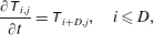 $$\begin{eqnarray}\displaystyle & \displaystyle \frac{\unicode[STIX]{x2202}\unicode[STIX]{x1D61B}_{i,j}}{\unicode[STIX]{x2202}t}=\unicode[STIX]{x1D61B}_{i+D,j},\quad i\leqslant D, & \displaystyle\end{eqnarray}$$
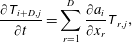 $$\begin{eqnarray}\displaystyle & \displaystyle \frac{\unicode[STIX]{x2202}\unicode[STIX]{x1D61B}_{i+D,j}}{\unicode[STIX]{x2202}t}=\mathop{\sum }_{r=1}^{D}\frac{\unicode[STIX]{x2202}a_{i}}{\unicode[STIX]{x2202}x_{r}}\unicode[STIX]{x1D61B}_{r,j}, & \displaystyle\end{eqnarray}$$
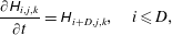 $$\begin{eqnarray}\displaystyle & \displaystyle \frac{\unicode[STIX]{x2202}\unicode[STIX]{x1D60F}_{i,j,k}}{\unicode[STIX]{x2202}t}=\unicode[STIX]{x1D60F}_{i+D,j,k},\quad i\leqslant D, & \displaystyle\end{eqnarray}$$
 $$\begin{eqnarray}\displaystyle & \displaystyle \frac{\unicode[STIX]{x2202}\unicode[STIX]{x1D60F}_{i+D,j,k}}{\unicode[STIX]{x2202}t}=\mathop{\sum }_{r=1}^{D}\frac{\unicode[STIX]{x2202}a_{i}}{\unicode[STIX]{x2202}x_{r}}\unicode[STIX]{x1D60F}_{r,j,k}+\mathop{\sum }_{r,s=1}^{D}\frac{\unicode[STIX]{x2202}^{2}a_{i}}{\unicode[STIX]{x2202}x_{r}\unicode[STIX]{x2202}x_{s}}\unicode[STIX]{x1D61B}_{r,j}\unicode[STIX]{x1D61B}_{s,k}, & \displaystyle\end{eqnarray}$$
where $\boldsymbol{a}$
is the acceleration calculated by solving Poisson’s equation. Note thus that we need to have access at all times to the gradient and the Hessian of the gravitational force. In these equations we have dropped the ‘
$\boldsymbol{a}$
is the acceleration calculated by solving Poisson’s equation. Note thus that we need to have access at all times to the gradient and the Hessian of the gravitational force. In these equations we have dropped the ‘ $m$
’ subscript for simplicity.
$m$
’ subscript for simplicity.
The actual time step implementation uses a splitting algorithm with a drift phase during half a time step where only spatial positions are modified, followed with a kick phase where only velocities are modified during a full time step using the acceleration computed after the drift, followed again by a drift during half a time step, where spatial positions are modified using the new velocities.
The first drift step or predictor is thus written
 $$\begin{eqnarray}\displaystyle & \displaystyle \boldsymbol{x}(t+\unicode[STIX]{x0394}t/2)=\boldsymbol{x}(t)+{\textstyle \frac{1}{2}}\boldsymbol{v}(t)\unicode[STIX]{x0394}t, & \displaystyle\end{eqnarray}$$
 $$\begin{eqnarray}\displaystyle & \displaystyle \unicode[STIX]{x1D61B}_{i,j}(t+\unicode[STIX]{x0394}t/2)=\unicode[STIX]{x1D61B}_{i,j}(t)+{\textstyle \frac{1}{2}}\unicode[STIX]{x1D61B}_{i+D,j}(t)\unicode[STIX]{x0394}t,\quad i\leqslant D, & \displaystyle\end{eqnarray}$$
 $$\begin{eqnarray}\displaystyle & \displaystyle \unicode[STIX]{x1D60F}_{i,j,k}(t+\unicode[STIX]{x0394}t/2)=\unicode[STIX]{x1D60F}_{i,j,k}(t)+{\textstyle \frac{1}{2}}\unicode[STIX]{x1D60F}_{i+D,j,k}\unicode[STIX]{x0394}t,\quad i\leqslant D, & \displaystyle\end{eqnarray}$$
after which Poisson’s equation is solved to compute the acceleration $\boldsymbol{a}(t+\unicode[STIX]{x0394}t/2)$
, its gradient and its Hessian. To compute the acceleration, we first need to estimate the phase-space distribution function
$\boldsymbol{a}(t+\unicode[STIX]{x0394}t/2)$
, its gradient and its Hessian. To compute the acceleration, we first need to estimate the phase-space distribution function $f(\boldsymbol{x},\boldsymbol{v},t+\unicode[STIX]{x0394}t/2)$
on the Eulerian grid. To map
$f(\boldsymbol{x},\boldsymbol{v},t+\unicode[STIX]{x0394}t/2)$
on the Eulerian grid. To map $f$
back to initial conditions (or previous stage after full remapping), we use the elements of metric as transformed by the predictor step.
$f$
back to initial conditions (or previous stage after full remapping), we use the elements of metric as transformed by the predictor step.
The kick phase reads
 $$\begin{eqnarray}\displaystyle & \displaystyle \boldsymbol{v}(t+\unicode[STIX]{x0394}t)=\boldsymbol{v}(t)+\boldsymbol{a}(t+\unicode[STIX]{x0394}t/2)\unicode[STIX]{x0394}t, & \displaystyle\end{eqnarray}$$
 $$\begin{eqnarray}\displaystyle & \displaystyle \unicode[STIX]{x1D61B}_{i+D,j}(t+\unicode[STIX]{x0394}t)=\unicode[STIX]{x1D61B}_{i,j}(t)+\mathop{\sum }_{r=1}^{D}\frac{\unicode[STIX]{x2202}a_{i}}{\unicode[STIX]{x2202}x_{r}}\unicode[STIX]{x1D61B}_{r,j}(t+\unicode[STIX]{x0394}t/2)\unicode[STIX]{x0394}t, & \displaystyle\end{eqnarray}$$
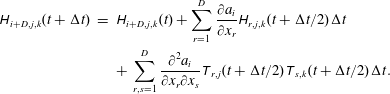 $$\begin{eqnarray}\displaystyle \unicode[STIX]{x1D60F}_{i+D,j,k}(t+\unicode[STIX]{x0394}t) & = & \displaystyle \unicode[STIX]{x1D60F}_{i+D,j,k}(t)+\mathop{\sum }_{r=1}^{D}\frac{\unicode[STIX]{x2202}a_{i}}{\unicode[STIX]{x2202}x_{r}}\unicode[STIX]{x1D60F}_{r,j,k}(t+\unicode[STIX]{x0394}t/2)\unicode[STIX]{x0394}t\nonumber\\ \displaystyle & & \displaystyle +\,\mathop{\sum }_{r,s=1}^{D}\frac{\unicode[STIX]{x2202}^{2}a_{i}}{\unicode[STIX]{x2202}x_{r}\unicode[STIX]{x2202}x_{s}}\unicode[STIX]{x1D61B}_{r,j}(t+\unicode[STIX]{x0394}t/2)\unicode[STIX]{x1D61B}_{s,k}(t+\unicode[STIX]{x0394}t/2)\unicode[STIX]{x0394}t.\end{eqnarray}$$
Finally the second drift phase, or corrector, is expressed as follows:
 $$\begin{eqnarray}\displaystyle & \displaystyle \boldsymbol{x}(t+\unicode[STIX]{x0394}t)=\boldsymbol{x}(t+\unicode[STIX]{x0394}t/2)+{\textstyle \frac{1}{2}}\boldsymbol{v}(t+\unicode[STIX]{x0394}t)\unicode[STIX]{x0394}t, & \displaystyle\end{eqnarray}$$
 $$\begin{eqnarray}\displaystyle & \displaystyle \unicode[STIX]{x1D61B}_{i,j}(t+\unicode[STIX]{x0394}t)=\unicode[STIX]{x1D61B}_{i,j}(t+\unicode[STIX]{x0394}t/2)+{\textstyle \frac{1}{2}}\unicode[STIX]{x1D61B}_{i+D,j}(t+\unicode[STIX]{x0394}t)\unicode[STIX]{x0394}t,\quad i\leqslant D, & \displaystyle\end{eqnarray}$$
 $$\begin{eqnarray}\displaystyle & \displaystyle \unicode[STIX]{x1D60F}_{i,j,k}(t+\unicode[STIX]{x0394}t)=\unicode[STIX]{x1D60F}_{i,j,k}(t+\unicode[STIX]{x0394}t/2)+{\textstyle \frac{1}{2}}\unicode[STIX]{x1D60F}_{i+D,j,k}(t+\unicode[STIX]{x0394}t)\unicode[STIX]{x0394}t,\quad i\leqslant D. & \displaystyle\end{eqnarray}$$
With our predictor–corrector scheme, it is possible to adopt a slowly variable time step. In this case, we use the following dynamical constraint (see, e.g. Alard & Colombi Reference Alard and Colombi2005; Colombi & Touma Reference Colombi and Touma2014),
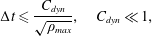 $$\begin{eqnarray}\displaystyle \unicode[STIX]{x0394}t\leqslant \frac{C_{dyn}}{\sqrt{\unicode[STIX]{x1D70C}_{max}}},\quad C_{dyn}\ll 1, & & \displaystyle\end{eqnarray}$$
where $\unicode[STIX]{x1D70C}_{max}=\text{max}_{x}\unicode[STIX]{x1D70C}(x)$
is the maximum value of the projected density,
$\unicode[STIX]{x1D70C}_{max}=\text{max}_{x}\unicode[STIX]{x1D70C}(x)$
is the maximum value of the projected density, $\unicode[STIX]{x1D70C}(x)\equiv \int f(x,v)\,\text{d}v$
. Note that for the tests performed in § 3, we used a constant time step, but this should not have critical effects on the numerical results.
$\unicode[STIX]{x1D70C}(x)\equiv \int f(x,v)\,\text{d}v$
. Note that for the tests performed in § 3, we used a constant time step, but this should not have critical effects on the numerical results.
2.5 Calculation of the force and its derivatives
In practice, the force is calculated on a grid and its gradient and Hessian estimated by simple finite difference methods.
In our 2-D phase-space implementation, the acceleration is calculated at discrete points $i$
with coordinate
$i$
with coordinate $x_{i}=x_{mid}+\unicode[STIX]{x0394}xi$
corresponding to the projection of the Eulerian phase-space grid. To estimate it, we first calculate the projected mass
$x_{i}=x_{mid}+\unicode[STIX]{x0394}xi$
corresponding to the projection of the Eulerian phase-space grid. To estimate it, we first calculate the projected mass $M(i)$
inside each pixel
$M(i)$
inside each pixel $i$
by summing up the phase-space density calculated at each point
$i$
by summing up the phase-space density calculated at each point $(i,j)$
of the Eulerian phase-space grid. In the present work we consider isolated systems in an empty space, which means that the acceleration at a given point
$(i,j)$
of the Eulerian phase-space grid. In the present work we consider isolated systems in an empty space, which means that the acceleration at a given point $x$
is simply proportional to the total mass at the right of point
$x$
is simply proportional to the total mass at the right of point $x$
minus the total mass at the left of
$x$
minus the total mass at the left of $x$
. This implies, within some trivial factor depending on code units
$x$
. This implies, within some trivial factor depending on code units
 $$\begin{eqnarray}\displaystyle a(i)=M_{total}-M_{left}(i)-M_{left}(i-1), & & \displaystyle\end{eqnarray}$$
with
 $$\begin{eqnarray}\displaystyle M_{left}(i)=\mathop{\sum }_{m\leqslant i}M(m), & & \displaystyle\end{eqnarray}$$
and where $M_{total}$
is the total mass of the system. Note thus that the mass in pixel
$M_{total}$
is the total mass of the system. Note thus that the mass in pixel $i$
does not contribute to
$i$
does not contribute to $a(i)$
as it is supposed to be distributed symmetrically inside itFootnote
3
. In a larger number of dimensions, Poisson’s equation is more complex to solve but this can be done on a fixed grid resolution with Fast Fourier Transform (FFT) methods, whether the system is spatially periodic or isolated as supposed here.
$a(i)$
as it is supposed to be distributed symmetrically inside itFootnote
3
. In a larger number of dimensions, Poisson’s equation is more complex to solve but this can be done on a fixed grid resolution with Fast Fourier Transform (FFT) methods, whether the system is spatially periodic or isolated as supposed here.
Our estimates of the first and second derivatives of the acceleration at the grid points are written
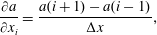 $$\begin{eqnarray}\displaystyle & \displaystyle \frac{\unicode[STIX]{x2202}a}{\unicode[STIX]{x2202}x_{i}}=\frac{a(i+1)-a(i-1)}{\unicode[STIX]{x0394}x}, & \displaystyle\end{eqnarray}$$
 $$\begin{eqnarray}\displaystyle & \displaystyle \frac{\unicode[STIX]{x2202}^{2}a}{\unicode[STIX]{x2202}x_{i}^{2}}=\frac{a(i+1)+a(i-1)-2a(i)}{(\unicode[STIX]{x0394}x)^{2}}, & \displaystyle\end{eqnarray}$$
which is equivalent to fitting the acceleration with a second-order polynomial on the three successive points corresponding to $i-1$
,
$i-1$
, $i$
and
$i$
and $i+1$
.
$i+1$
.
To compute the force at an arbitrary point of the computing domain, we perform dual TSC (triangular shaped cloud, see e.g. Hockney & Eastwood Reference Hockney and Eastwood1988) interpolation from the grid, i.e.
 $$\begin{eqnarray}\displaystyle & \displaystyle a(x)={\textstyle \frac{1}{2}}\left({\textstyle \frac{1}{2}}-w\right)^{2}a(i-1)+\left({\textstyle \frac{3}{4}}-w^{2}\right)a(i)+{\textstyle \frac{1}{2}}\left({\textstyle \frac{1}{2}}+w\right)^{2}a(i+1), & \displaystyle\end{eqnarray}$$
 $$\begin{eqnarray}\displaystyle & \displaystyle i=\lfloor (x-x_{mid})/\unicode[STIX]{x0394}x\rceil , & \displaystyle\end{eqnarray}$$
 $$\begin{eqnarray}\displaystyle & \displaystyle w=(x-x_{mid})/\unicode[STIX]{x0394}x-i, & \displaystyle\end{eqnarray}$$
and likewise for its gradient and its second derivative. Note that we also tested linear interpolation, which leads in practice to nearly the same results as TSC for all the numerical tests we discuss in next section.
Clearly, the way we estimate the force and its successive derivatives is probably too naive but actually works pretty well for all the experiments we did so we did not attempt to improve this part of our algorithm. However, this should be investigated in a future work.
3 Numerical experiments
Parameters of the simulations performed in this work, namely the grid cell size, $\unicode[STIX]{x1D6E5}=\unicode[STIX]{x0394}x=\unicode[STIX]{x0394}y$
, the initial separation between each metric element,
$\unicode[STIX]{x1D6E5}=\unicode[STIX]{x0394}x=\unicode[STIX]{x0394}y$
, the initial separation between each metric element, $\unicode[STIX]{x1D6E5}_{m}=\unicode[STIX]{x0394}x_{m}=\unicode[STIX]{x0394}y_{m}$
, the number of subcycles,
$\unicode[STIX]{x1D6E5}_{m}=\unicode[STIX]{x0394}x_{m}=\unicode[STIX]{x0394}y_{m}$
, the number of subcycles, $n_{s}$
, between resamplings and the approximate total Central Processing Unit (CPU) time expressed in units of the time spent for simulation I. The calculation of
$n_{s}$
, between resamplings and the approximate total Central Processing Unit (CPU) time expressed in units of the time spent for simulation I. The calculation of $t_{CPU}$
was performed for the simulations with initial conditions corresponding to the random set of stationary clouds as described in § 3.2, but the results do not change drastically for other initial conditions. A space separates the runs performed with Vlamet (I–XI) from those performed with the standard splitting algorithm (XII–XVI). Additionally, the time step
$t_{CPU}$
was performed for the simulations with initial conditions corresponding to the random set of stationary clouds as described in § 3.2, but the results do not change drastically for other initial conditions. A space separates the runs performed with Vlamet (I–XI) from those performed with the standard splitting algorithm (XII–XVI). Additionally, the time step $\unicode[STIX]{x0394}t$
was chosen constant, given by
$\unicode[STIX]{x0394}t$
was chosen constant, given by $\unicode[STIX]{x0394}t=0.01$
,
$\unicode[STIX]{x0394}t=0.01$
, $0.01$
and
$0.01$
and $0.0025$
for the stationary, Gaussian and random set of halos, respectively. The two last choices come from the constraints on the time step obtained in the waterbag runs by Colombi & Touma (Reference Colombi and Touma2014).
$0.0025$
for the stationary, Gaussian and random set of halos, respectively. The two last choices come from the constraints on the time step obtained in the waterbag runs by Colombi & Touma (Reference Colombi and Touma2014).
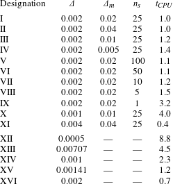
To test the method, we performed an ensemble of simulations of which the parameters are listed in table 1. In § 3.2, we compare the results obtained with Vlamet to the standard splitting algorithm of Cheng & Knorr (Reference Cheng and Knorr1976) with cubic B-spline interpolation as well as the extremely accurate entropy conserving waterbag simulations of Colombi & Touma (Reference Colombi and Touma2014, hereafter CT14). Before going into the details of these comparisons, we first provide in § 3.1 additional technical information on the performances of Vlamet and of the splitting algorithmFootnote 4 . In particular, we discuss parallelisation issues as well as extension to a higher number of dimensions.
Accelerations of our implementations of Vlamet (in red) and of the splitting algorithm (in black) as functions of the number of cores on a shared memory architecture with OpenMP library. The plot is performed for the parameters corresponding to runs I and XVI in table 1, starting from an ensemble of stationary clouds. Perfect speed up is represented as a dotted line.

3.1 Performance: parallel scaling and computing cost
Both Vlamet and the splitting algorithm are parallelised on shared memory architecture using OpenMP library, but no attempt has been made to optimise cash memory, so there is still room for improvement. Parallel scaling is displayed in figure 6, which shows that the two codes present a reasonable speed up, greater than 10 on 32 cores. The scaling is slightly better for the metric code than for the splitting algorithm but this comparison is irrelevant without further optimisation. The main point here is to show that OpenMP parallelisation is rather straightforward for Vlamet, while it is already well known that both distributed and shared memory parallelisations are not a problem for the splitting algorithm (see, e.g. Crouseilles et al. Reference Crouseilles, Latu and Sonnendrücker2009).
As an additional note, but this is something we leave for future work, there is in principle no particular difficulty in parallelising Vlamet on a distributed memory architecture with the Message Passing Interface (MPI) library. Except for solving Poisson’s equation and for cubic B-spline interpolation that we will discuss, all the operations performed in the algorithm, including the percolation process, are of local nature, hence trivially compatible with domain decomposition. In four- and six-dimensional phase space, introducing a k-d tree structure to focus on important regions of phase space is also quite standard in parallel programming. The solution to Poisson equation is well known in many parallel implementations. For instance there exist parallel fast Fourier transform libraries such as FFTW to compute the gravitational potential on a fixed resolution grid. As for spline interpolation, a domain decomposition implementation is possible using the method proposed by Crouseilles et al. (Reference Crouseilles, Latu and Sonnendrücker2009). In this case, interpolation is localised to each domain by using Hermite boundary conditions between the domains with an ad hoc reconstruction of the derivatives. In this implementation, each domain would for instance correspond to a leaf of the k-d tree mentioned above. Of course, as long as we did not actually implement the algorithm on distributed memory architecture, this discussion stays at the speculative level.
In terms of total computational time, interesting conclusions can be derived from examination of the fifth column of table 1, which indicates, for each run, the approximate total CPU cost in units of simulation I. Neglecting the Poisson equation resolution step, both Vlamet and the splitting algorithm are expected in general to scale approximately like the number $n_{cells}\propto \unicode[STIX]{x1D6E5}^{-2D}$
of cells in the grid representing phase space, where
$n_{cells}\propto \unicode[STIX]{x1D6E5}^{-2D}$
of cells in the grid representing phase space, where $D$
(here equal to unity) is the number of dimensions of space. This is approximately the case in table 1 if
$D$
(here equal to unity) is the number of dimensions of space. This is approximately the case in table 1 if $\unicode[STIX]{x1D6E5}$
is small enough. The cost also increases for Vlamet when resamplings of the phase-space distribution function are more frequent (in practice, if
$\unicode[STIX]{x1D6E5}$
is small enough. The cost also increases for Vlamet when resamplings of the phase-space distribution function are more frequent (in practice, if $n_{s}\lesssim 10$
for the runs we did) or when the element of metric density increases (in practice, if
$n_{s}\lesssim 10$
for the runs we did) or when the element of metric density increases (in practice, if $\unicode[STIX]{x1D6E5}_{m}\lesssim 10\unicode[STIX]{x1D6E5}$
for the runs we did).
$\unicode[STIX]{x1D6E5}_{m}\lesssim 10\unicode[STIX]{x1D6E5}$
for the runs we did).
When it comes to really compare Vlamet to the standard splitting algorithm, we focus on single thread runs, assuming that full parallelisation is equally optimal on both algorithms. We noticed that with the same spatial resolution $\unicode[STIX]{x1D6E5}$
, Vlamet is approximately
$\unicode[STIX]{x1D6E5}$
, Vlamet is approximately $\unicode[STIX]{x1D6FC}_{slower}=1.4{-}2$
times slower than the splitting algorithm for
$\unicode[STIX]{x1D6FC}_{slower}=1.4{-}2$
times slower than the splitting algorithm for $n_{s}\gtrsim 25$
and
$n_{s}\gtrsim 25$
and $\unicode[STIX]{x1D6E5}_{m}/\unicode[STIX]{x1D6E5}\gtrsim 2.5$
. How these estimates generalise to four and six dimensions remains an open question, but we can try to infer some rough estimates. From now on we restrict to 6-D phase space. In this case, the critical step in Vlamet is the cubic spline interpolation during the resampling phase, which is expected to be approximately 171 times more costly than a step of the standard splitting algorithm, as discussed in introduction of § 2.2. The rest of the algorithm, on the other hand, should perform comparably well to the splitting scheme, i.e. should be
$\unicode[STIX]{x1D6E5}_{m}/\unicode[STIX]{x1D6E5}\gtrsim 2.5$
. How these estimates generalise to four and six dimensions remains an open question, but we can try to infer some rough estimates. From now on we restrict to 6-D phase space. In this case, the critical step in Vlamet is the cubic spline interpolation during the resampling phase, which is expected to be approximately 171 times more costly than a step of the standard splitting algorithm, as discussed in introduction of § 2.2. The rest of the algorithm, on the other hand, should perform comparably well to the splitting scheme, i.e. should be $\unicode[STIX]{x1D6FC}_{loss}$
times slower with
$\unicode[STIX]{x1D6FC}_{loss}$
times slower with $\unicode[STIX]{x1D6FC}_{loss}$
of the order of unity. Hence we expect, in six dimensions, a factor
$\unicode[STIX]{x1D6FC}_{loss}$
of the order of unity. Hence we expect, in six dimensions, a factor $\unicode[STIX]{x1D6FC}_{slower}^{6D}\simeq (n_{s}\times \unicode[STIX]{x1D6FC}_{loss}+171)/n_{s}$
between Vlamet and the standard splitting algorithm, that is
$\unicode[STIX]{x1D6FC}_{slower}^{6D}\simeq (n_{s}\times \unicode[STIX]{x1D6FC}_{loss}+171)/n_{s}$
between Vlamet and the standard splitting algorithm, that is $\unicode[STIX]{x1D6FC}_{slower}^{6D}$
ranging from about 2 in the optimistic cases (e.g.
$\unicode[STIX]{x1D6FC}_{slower}^{6D}$
ranging from about 2 in the optimistic cases (e.g. $\unicode[STIX]{x1D6FC}_{loss}\simeq 1$
and
$\unicode[STIX]{x1D6FC}_{loss}\simeq 1$
and $n_{s}=200$
) to approximately 20 in the pessimistic ones (e.g.
$n_{s}=200$
) to approximately 20 in the pessimistic ones (e.g. $\unicode[STIX]{x1D6FC}_{loss}=10$
and
$\unicode[STIX]{x1D6FC}_{loss}=10$
and $n_{s}=15$
). While a factor as large as 20 might seem potentially prohibitive, we remind the reader that our code is supposed to be less diffusive than the splitting algorithm, as we shall illustrate next, hence should require less spatial resolution. A simple factor 2 in resolution corresponding to a gain of approximately
$n_{s}=15$
). While a factor as large as 20 might seem potentially prohibitive, we remind the reader that our code is supposed to be less diffusive than the splitting algorithm, as we shall illustrate next, hence should require less spatial resolution. A simple factor 2 in resolution corresponding to a gain of approximately $2^{6}=64$
in speed and memory would make Vlamet extremely competitive.
$2^{6}=64$
in speed and memory would make Vlamet extremely competitive.
3.2 Test runs: comparisons between codes
Before going further, it is important here to specify the units in which we are solving the Vlasov–Poisson equations. Our choice is the same as in CT14, i.e. we are studying the following system of equations:
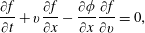 $$\begin{eqnarray}\displaystyle & \displaystyle \frac{\unicode[STIX]{x2202}f}{\unicode[STIX]{x2202}t}+v\frac{\unicode[STIX]{x2202}f}{\unicode[STIX]{x2202}x}-\frac{\unicode[STIX]{x2202}\unicode[STIX]{x1D719}}{\unicode[STIX]{x2202}x}\frac{\unicode[STIX]{x2202}f}{\unicode[STIX]{x2202}v}=0, & \displaystyle\end{eqnarray}$$
 $$\begin{eqnarray}\displaystyle & \displaystyle \frac{\unicode[STIX]{x2202}^{2}\unicode[STIX]{x1D719}}{\unicode[STIX]{x2202}x^{2}}=2\unicode[STIX]{x1D70C}=2\int f(x,v,t)\,\text{d}v. & \displaystyle\end{eqnarray}$$
To test Vlamet, three kinds of initial conditions were considered, namely the thermal equilibrium solution, Gaussian initial conditions and a random set of stationary clouds, as detailed below.
-
(i) The thermal equilibrium solution (Spitzer Reference Spitzer1942; Camm Reference Camm1950; Rybicki Reference Rybicki1971) reads
(3.3)In practice, we set
$$\begin{eqnarray}\displaystyle f_{S}(x,v)=\frac{\unicode[STIX]{x1D70C}_{S}}{\left[\text{ch}\left(\sqrt{\sqrt{2\unicode[STIX]{x03C0}}\unicode[STIX]{x1D70C}_{S}/\unicode[STIX]{x1D70E}_{S}}x\right)\right]^{2}}\exp \left[-\frac{1}{2}\left(\frac{v}{\unicode[STIX]{x1D70E}_{S}}\right)^{2}\right]. & & \displaystyle\end{eqnarray}$$
(3.4)with the apodising function
$$\begin{eqnarray}\displaystyle f_{ini}(x,v)=f_{S}(x,v)g_{\unicode[STIX]{x1D702}}[f_{S}(x,v)], & & \displaystyle\end{eqnarray}$$
$g_{\unicode[STIX]{x1D702}}$
given by (3.5)For the runs performed in this paper, we took
$$\begin{eqnarray}\displaystyle g_{\unicode[STIX]{x1D702}}(y)=\unicode[STIX]{x1D702}\max \left[1+2\text{ th}\left(\frac{y-\unicode[STIX]{x1D702}}{\unicode[STIX]{x1D702}}\right),0\right]. & & \displaystyle\end{eqnarray}$$
$\unicode[STIX]{x1D70C}_{S}=4$
,
$\unicode[STIX]{x1D70E}_{S}=0.2$
and
$\unicode[STIX]{x1D702}=0.02$
, which means that the maximum projected density of the system is
$\unicode[STIX]{x1D70C}_{max}\simeq 2$
. The harmonic dynamical time corresponding to such a density is, in our units, (3.6)The simulation was run up to
$$\begin{eqnarray}\displaystyle T_{dyn}=\frac{2\unicode[STIX]{x03C0}}{\sqrt{2\unicode[STIX]{x1D70C}_{max}}}. & & \displaystyle\end{eqnarray}$$
$t=100$
, which corresponds to
$100/T_{dyn}\simeq 32$
dynamical times. Thermal equilibrium is stable and hence represents a crucial test for a code, which has to be able to maintain it accurately. Figure 7 shows how Vlamet performs for runs I, II, III and IV, when considering the difference
$\unicode[STIX]{x1D6FF}f=f(x,v,t)-f_{ini}(x,v)$
at
$t=100$
, i.e. checks the behaviour of the code when changing the distance
$\unicode[STIX]{x1D6E5}_{m}$
between metric elements while keeping resolution fixed to
$\unicode[STIX]{x1D6E5}=0.002$
. For comparison, a curve corresponding to the splitting algorithm run XVI is also shown at same resolution
$\unicode[STIX]{x1D6E5}$
. As expected, Vlamet performs very well, as long as
$\unicode[STIX]{x1D6E5}_{m}/\unicode[STIX]{x1D6E5}$
remains sufficiently small,
$\unicode[STIX]{x1D6E5}_{m}/\unicode[STIX]{x1D6E5}\lesssim 10$
, to avoid too large errors on the reconstruction of Lagrangian positions from the metric elements. We also checked that
$|\unicode[STIX]{x1D6FF}f|$
decreases when augmenting the spatial resolution of the simulation. Note that the splitting algorithm seems to perform even better than Vlamet, as suggested by the turquoise curve in figure 7(b). A residual error remains in all cases, since there is a clear convergence to a non-zero
$\unicode[STIX]{x1D6FF}f$
. From performing a run similar to I but with a twice larger time step and another one with a truncation parameter
$\unicode[STIX]{x1D702}$
twenty times smaller, we see that this small residual can be attributed to the finite value of the time step and especially the (rather strong) truncation of
$f$
with apodising function
$g_{\unicode[STIX]{x1D702}}$
, which implies that the initial conditions constructed this way do not correspond exactly to thermal equilibrium. Although we do not have any rigorous mathematical argument to support the claim that follows, decreasing
$\unicode[STIX]{x0394}t$
and the value of
$\unicode[STIX]{x1D702}$
should make this residual tend to zero, both for Vlamet and the splitting algorithm, provided that resolution
$1/\unicode[STIX]{x1D6E5}$
becomes also arbitrarily large and the ratio
$\unicode[STIX]{x1D6E5}_{m}/\unicode[STIX]{x1D6E5}$
is kept sufficiently small.
-
(ii) Gaussian initial conditions are given by
(3.7)
$$\begin{eqnarray}\displaystyle f_{ini}(x,v) & = & \displaystyle G(x,v),\quad x^{2}+v^{2}\leqslant {\mathcal{R}}^{2},\end{eqnarray}$$
(3.8)with
$$\begin{eqnarray}\displaystyle & = & \displaystyle G(x,v)\max \left[1+2\text{ th}\left(\frac{{\mathcal{R}}-\sqrt{x^{2}+v^{2}}}{\unicode[STIX]{x1D702}_{G}}\right),0\right],\quad x^{2}+v^{2}>{\mathcal{R}}^{2},\nonumber\\ \displaystyle & & \displaystyle\end{eqnarray}$$
(3.9)In practice, to compare the output of Vlamet to the waterbag result of CT14, we take
$$\begin{eqnarray}\displaystyle G(x,v)\equiv \unicode[STIX]{x1D70C}_{G}\exp \left(-\frac{1}{2}\frac{x^{2}+v^{2}}{\unicode[STIX]{x1D70E}_{G}^{2}}\right). & & \displaystyle\end{eqnarray}$$
${\mathcal{R}}=1$
,
$\unicode[STIX]{x1D70C}_{G}=4$
,
$\unicode[STIX]{x1D70E}_{G}=0.2$
and
$\unicode[STIX]{x1D702}_{G}=0.02$
, which makes the total mass of the system approximately equal to unity for a Gaussian truncated at 5 sigma. The measured maximum projected density of this system, is, after relaxation,
$\unicode[STIX]{x1D70C}_{max}=2.95$
, so simulating this system up to
$t=100$
corresponds to following it during approximately 39 dynamical times according to equation (3.6). Figure 8 shows, at various times, the phase-space distribution function obtained from run I and the waterbag run Gaussian84 of CT14. The agreement between both simulations seems visually close to perfect. A more careful examination of the details of the phase-space distribution function shows small deviations which can be reduced by augmenting the resolution of the Vlamet run. This is illustrated by figure 9, which displays on a small interval, the projected density for runs I, X, XI (different resolutions
$\unicode[STIX]{x1D6E5}$
but fixed
$n_{s}=25$
and fixed ratio
$\unicode[STIX]{x1D6E5}_{m}/\unicode[STIX]{x1D6E5}=10$
) and Gaussian84. What is particularly interesting in this figure are the turquoise curves corresponding to runs performed with the splitting algorithm, namely XII, XIV and XVI. We notice a very good match between Vlamet and the splitting algorithm but only if this latter is run at twice the resolution of Vlamet! This figure already demonstrates the significantly weaker level of diffusion of Vlamet compared to the splitting algorithm.
-
(iii) The ensemble of stationary clouds corresponds to a set of halos following the stationary solution (3.3), created exactly as in CT14. In particular, their profile follows equation (3.3) with
$\unicode[STIX]{x1D70C}_{S}=6$
and their velocity dispersion,
$\unicode[STIX]{x1D70E}_{S}$
, ranges in the interval
$[0.005,0.1]$
. The components are added on the top of each other in phase space, to obtain the desired initial distribution function
$f_{ini}(x,v)$
, which is apodised as in equation (3.4) with
$\unicode[STIX]{x1D702}=0.05$
. The interesting fact about this system is that it was found experimentally by CT14 to be chaotic. In figure 10, the phase-space distribution function is shown at various times for simulation I and run Random of CT14. At
$t=25$
, the agreement between both simulations is impressive, despite the fact that the phase-space distribution function is sampled with only three waterbags in the Random run of CT14. At
$t=80$
, the system presents remarkable structures: some halos have been destroyed by tidal effects and a complex filamentary structure has grown. At this time, the Vlamet and the waterbag runs diverge from each other, but remain still in agreement at the macroscopic level. The fact that the simulations diverge from each other is not surprising since the run performed by CT14 samples the phase-space distribution function with only 3 waterbags. The differences are also amplified by the intrinsic chaotic nature of the system. Note that the Vlamet run is subject, at this point, to significant aliasing effects. For instance, the minimum value of the measured phase-space distribution function on figure 10(e) is equal to
$f_{min}=-0.38$
, which is of rather large magnitude given the maximum theoretical value of
$f$
,
$f_{max}=6$
. These aliasing effects are inherent to the spline interpolation procedure we are using. Importantly, aliasing effects do not affect the dynamical properties of the system: increasing the resolution or decreasing it (runs X and XI) does not change the results significantly, despite the chaotic nature of the system, except at very small scales close to spatial resolution, of course. As illustrated below quantitatively, similarly to the Gaussian case discussed above, simulations with the splitting algorithm provide comparable results to Vlamet but only if performed at better resolution.











Deviation from stationarity for simulations with $\unicode[STIX]{x1D6E5}=0.002$
. (a) The difference
$\unicode[STIX]{x1D6E5}=0.002$
. (a) The difference $\unicode[STIX]{x1D6FF}f$
between the phase-space density measured at
$\unicode[STIX]{x1D6FF}f$
between the phase-space density measured at $t=100$
and the initial one for simulation I. Darker regions correspond to larger values of
$t=100$
and the initial one for simulation I. Darker regions correspond to larger values of $\unicode[STIX]{x1D6FF}f$
, which ranges in the interval
$\unicode[STIX]{x1D6FF}f$
, which ranges in the interval $\unicode[STIX]{x1D6FF}f\in [-0.0014,0.0014]$
. (b) The value of
$\unicode[STIX]{x1D6FF}f\in [-0.0014,0.0014]$
. (b) The value of $\unicode[STIX]{x1D6FF}f(x,0)$
is plotted for simulations I, II, III, IV (i.e. varying inter-element of metric distance
$\unicode[STIX]{x1D6FF}f(x,0)$
is plotted for simulations I, II, III, IV (i.e. varying inter-element of metric distance $\unicode[STIX]{x1D6E5}_{m}$
while keeping spatial resolution
$\unicode[STIX]{x1D6E5}_{m}$
while keeping spatial resolution $\unicode[STIX]{x1D6E5}=0.002$
fixed) and XVI. Note that the purple and blue curves nearly superpose on each other.
$\unicode[STIX]{x1D6E5}=0.002$
fixed) and XVI. Note that the purple and blue curves nearly superpose on each other.

Phase-space density in the simulations with Gaussian initial conditions. The simulation I with the metric method is compared to a waterbag run of Colombi & Touma (Reference Colombi and Touma2014). In the latter case, the phase-space distribution function is represented with 84 waterbags.

Projected density in the simulations with Gaussian initial conditions: detail. The simulations performed with Vlamet, I, X and XI are compared to the results obtained with the splitting algorithm, XII, XIV and XVI, as well as a waterbag run of Colombi & Touma (Reference Colombi and Touma2014), which is supposed to represent the ‘exact’ solution. Note that while the waterbag measurements are displayed at the fine grained level, the results from the Vlamet and the splitting algorithm runs are shown at the grid resolution, $\unicode[STIX]{x1D6E5}$
.
$\unicode[STIX]{x1D6E5}$
.

Phase-space density in the simulations with random initial conditions. The simulation I with the metric method is compared to a waterbag run of Colombi & Touma (Reference Colombi and Touma2014). In the latter case, the phase-space distribution function is represented with only with three waterbag levels.

To perform more quantitative tests, we checked for conservation of total energy, which can be conveniently written
 $$\begin{eqnarray}\displaystyle E=\frac{1}{2}\int v^{2}f(x,v,t)\,\text{d}x\,\text{d}v-\frac{1}{4}\int [a(x,t)^{2}-M_{total}^{2}]\,\text{d}x, & & \displaystyle\end{eqnarray}$$
where $a(x,t)$
is the gravitational force and
$a(x,t)$
is the gravitational force and $M_{total}$
the total mass. These integral are computed directly as sums on the grid used to sample the phase-space distribution function and the force. In addition, we check for conservation of the following Casimir
$M_{total}$
the total mass. These integral are computed directly as sums on the grid used to sample the phase-space distribution function and the force. In addition, we check for conservation of the following Casimir
 $$\begin{eqnarray}\displaystyle S=-\int f(x,v)\log |f(x,v)|\,\text{d}x\,\text{d}v, & & \displaystyle\end{eqnarray}$$
which is numerically estimated the same way as total energy. This quantity would reduce to Gibbs entropy if positivity of the phase-space distribution function was preserved. While we know it is not rigorously correct, we shall still designate $S$
by entropy. We also tested for total mass conservation, as well as
$S$
by entropy. We also tested for total mass conservation, as well as $L^{1}$
and
$L^{1}$
and $L^{2}$
norms, but do not show the results here to avoid superfluous content. Indeed, energy and entropy were found in practice to be sufficiently representative of the system when it comes to test the accuracy of Vlamet.
$L^{2}$
norms, but do not show the results here to avoid superfluous content. Indeed, energy and entropy were found in practice to be sufficiently representative of the system when it comes to test the accuracy of Vlamet.
Figures 11–13 show $E$
and
$E$
and $S$
in the simulations we performed for the stationary, the Gaussian and the random set of halos, respectively. These figures allow us to test thoroughly the performance of Vlamet and to compare it to the splitting algorithm. They are supplemented with figure 14, which displays the corresponding maximum mismatch between the Lagrangian positions predicates from neighbouring metric elements, as defined in § 2.3.3.
$S$
in the simulations we performed for the stationary, the Gaussian and the random set of halos, respectively. These figures allow us to test thoroughly the performance of Vlamet and to compare it to the splitting algorithm. They are supplemented with figure 14, which displays the corresponding maximum mismatch between the Lagrangian positions predicates from neighbouring metric elements, as defined in § 2.3.3.
Conservation of energy (a,c,e) and entropy (b,d,f) in the stationary runs. Each line of panels corresponds to varying one parameter of the simulations as listed in table 1. In the first line of panels, we vary the elements of metric sampling, $\unicode[STIX]{x1D6E5}_{m}=\unicode[STIX]{x0394}x_{m}=\unicode[STIX]{x0394}v_{m}$
, while keeping other parameters, in particular spatial resolution
$\unicode[STIX]{x1D6E5}_{m}=\unicode[STIX]{x0394}x_{m}=\unicode[STIX]{x0394}v_{m}$
, while keeping other parameters, in particular spatial resolution $\unicode[STIX]{x1D6E5}=\unicode[STIX]{x0394}x=\unicode[STIX]{x0394}v$
, fixed. In the second line of panels, it is the number of time steps
$\unicode[STIX]{x1D6E5}=\unicode[STIX]{x0394}x=\unicode[STIX]{x0394}v$
, fixed. In the second line of panels, it is the number of time steps $n_{s}$
between each resampling which changes. Finally, in the last line of panels, overall resolution is changed, i.e. both
$n_{s}$
between each resampling which changes. Finally, in the last line of panels, overall resolution is changed, i.e. both $\unicode[STIX]{x1D6E5}$
and
$\unicode[STIX]{x1D6E5}$
and $\unicode[STIX]{x1D6E5}_{m}$
while keeping the ratio
$\unicode[STIX]{x1D6E5}_{m}$
while keeping the ratio $\unicode[STIX]{x1D6E5}_{m}/\unicode[STIX]{x1D6E5}$
fixed. For comparison, results from the splitting algorithm are also displayed as turquoise curves as indicated on each panel. In the latter case, the only parameter of interest is spatial resolution
$\unicode[STIX]{x1D6E5}_{m}/\unicode[STIX]{x1D6E5}$
fixed. For comparison, results from the splitting algorithm are also displayed as turquoise curves as indicated on each panel. In the latter case, the only parameter of interest is spatial resolution $\unicode[STIX]{x1D6E5}$
.
$\unicode[STIX]{x1D6E5}$
.

Conservation of energy (a,c,e) and entropy (b,d,f) in the Gaussian runs, similarly as in figure 11. In (a,c,e), energy conservation of the splitting algorithm is plotted only for run XVI, but other runs (XII, XIII, XIV and XV) would provide nearly indistinguishable results given the interval of values investigated.

Conservation of energy (a,c,e) and entropy (b,d,f) in the random set of halos runs, similarly as in figure 11. Again, energy conservation of the splitting algorithm is plotted only for run XVI, because other runs would provide nearly indistinguishable results.

The maximum reconstructed displacement mismatch between neighbouring elements of metric, $E_{map}$
, as defined in § 2.3.3, as a function of time for the Vlamet runs considered in the energy and entropy plots shown in previous figures.
$E_{map}$
, as defined in § 2.3.3, as a function of time for the Vlamet runs considered in the energy and entropy plots shown in previous figures. $E_{map}$
is expressed in units of spatial resolution,
$E_{map}$
is expressed in units of spatial resolution, $\unicode[STIX]{x1D6E5}$
.
$\unicode[STIX]{x1D6E5}$
.

The most striking result when examining figures 12 and 13 is the superior behaviour of Vlamet compared to the standard splitting method with respect to entropy, in agreement with the preliminary conclusions driven from the analysis of figure 9. Indeed, to obtain comparable entropy conservation in Vlamet and the splitting algorithm, it is required to have a higher spatial resolution in the latter. Of course, the results depend on the choice of $n_{s}$
and of the ratio
$n_{s}$
and of the ratio $\unicode[STIX]{x0394}x_{m}/\unicode[STIX]{x1D6E5}$
. For instance, Vlamet runs with
$\unicode[STIX]{x0394}x_{m}/\unicode[STIX]{x1D6E5}$
. For instance, Vlamet runs with $n_{s}=25$
and
$n_{s}=25$
and $\unicode[STIX]{x0394}x_{m}/\unicode[STIX]{x1D6E5}=10$
perform as well as the splitting algorithm with twice the spatial resolution. But if
$\unicode[STIX]{x0394}x_{m}/\unicode[STIX]{x1D6E5}=10$
perform as well as the splitting algorithm with twice the spatial resolution. But if $n_{s}$
is increased to 100, it is required to increase the resolution by a factor as large as 2.8 (figure 13
d) or 4 (figure 12
d) in the splitting algorithm to perform as well as Vlamet. The price to pay might be energy conservation, which is in general not as good in Vlamet as in the splitting algorithm, that preserves energy at a level better than
$n_{s}$
is increased to 100, it is required to increase the resolution by a factor as large as 2.8 (figure 13
d) or 4 (figure 12
d) in the splitting algorithm to perform as well as Vlamet. The price to pay might be energy conservation, which is in general not as good in Vlamet as in the splitting algorithm, that preserves energy at a level better than ${\sim}10^{-5}$
regardless of initial conditions and spatial resolution. However, energy conservation violation in Vlamet can be kept under control with the appropriate combination of parameters
${\sim}10^{-5}$
regardless of initial conditions and spatial resolution. However, energy conservation violation in Vlamet can be kept under control with the appropriate combination of parameters $n_{s}$
and ratio
$n_{s}$
and ratio $\unicode[STIX]{x1D6E5}_{m}/\unicode[STIX]{x1D6E5}$
, as discussed further below. On the same ground, we notice, when examining figure 11, that the splitting algorithm seems to preserve better the thermal equilibrium solution than Vlamet, as already noticed in figure 7(b), unless
$\unicode[STIX]{x1D6E5}_{m}/\unicode[STIX]{x1D6E5}$
, as discussed further below. On the same ground, we notice, when examining figure 11, that the splitting algorithm seems to preserve better the thermal equilibrium solution than Vlamet, as already noticed in figure 7(b), unless $n_{s}$
or/and
$n_{s}$
or/and $\unicode[STIX]{x1D6E5}_{m}/\unicode[STIX]{x1D6E5}$
are chosen small enough. However, one has to be aware that the smoothness of the thermal equilibrium solution provides a very good ground for the splitting algorithm.
$\unicode[STIX]{x1D6E5}_{m}/\unicode[STIX]{x1D6E5}$
are chosen small enough. However, one has to be aware that the smoothness of the thermal equilibrium solution provides a very good ground for the splitting algorithm.
Further investigation of figures 11–14 allows us to study more in detail how Vlamet behaves with the various control parameters:
-
(1) Increasing overall resolution, i.e. decreasing
$\unicode[STIX]{x1D6E5}=\unicode[STIX]{x0394}x=\unicode[STIX]{x0394}y$
and
$\unicode[STIX]{x1D6E5}_{m}=\unicode[STIX]{x0394}x_{m}=\unicode[STIX]{x0394}y_{m}$
by some factor improves both energy conservation and entropy conservation, as can be seen from last line of panels of all the figures, as expected. Note that adopting
$\unicode[STIX]{x0394}x=\unicode[STIX]{x0394}y$
and
$\unicode[STIX]{x0394}x_{m}=\unicode[STIX]{x0394}y_{m}$
as we did in this work is not necessarily optimal, but is a natural choice in the code units if the total mass of the system is of the order of unity. -
(2) Changing the resampling frequency parameter
$n_{s}$
affects both entropy and energy, but to a much larger extent the former than the latter. In particular, increasing
$n_{s}$
up to 100 clearly improves entropy at an acceptable cost for energy conservation, of which the violation remains below the
${\sim}5\times 10^{-4}$
level, as can be seen from the second line of panels of figures 11–13. This is not surprising: performing less frequent resamplings of the phase-space distribution function decreases diffusion and aliasing, which is good for entropy conservation, but it worsens energy conservation, because (i) the error on the reconstruction of Lagrangian coordinates increases (middle line of panels in figure 14) and (ii) the phase-space distribution function is sampled more approximately during subcycles. While effect (i) can be reduced by augmenting the metric elements density as discussed below, effect (ii) always remains, which prevents arbitrarily large values of
$n_{s}$
. -
(3) Sparse sampling the elements of metric, i.e. increasing
$\unicode[STIX]{x1D6E5}_{m}$
, augments the error in the Lagrangian coordinates reconstruction (first line of panels in figure 14). This affects energy conservation but not so much the entropy (except for the stationary simulations, which nevertheless preserve entropy at a level better than
$10^{-3}$
). Entropy is indeed mainly sensitive to spatial resolution, i.e. the value of
$\unicode[STIX]{x1D6E5}$
, and as stated just above, to the frequency of resamplings. For the experiments we did, we find that the ratio
$\unicode[STIX]{x1D6E5}_{m}/\unicode[STIX]{x1D6E5}$
should not exceed a factor 10, and the smaller it is, the better the results, obviously. For instance, using
$\unicode[STIX]{x1D6E5}_{m}/\unicode[STIX]{x1D6E5}\lesssim 5$
leads to energy conserved better than
${\sim}5\times 10^{-5}$
for
$\unicode[STIX]{x1D6E5}=0.002$
and
$n_{s}=25$
. Being aware that the gain in memory is already a factor
$2.5^{6}=244$
in six dimensions when sparse sampling the elements of metric by a factor
$2.5$
in each direction compared to the computational grid, it is obviously wise to keep the elements of metric sampling sufficiently dense at the price of a small increase of the computational cost (a factor of the order of 1.4 in 2-D phase space for
$\unicode[STIX]{x1D6E5}_{m}/\unicode[STIX]{x1D6E5}=2.5$
, according to fifth column of table 1). Furthermore, a higher density of metric elements allows for a larger value of
$n_{s}$
.




4 Conclusion
We have proposed and tested a new Vlasov solver, Vlamet, which uses small elements of metric to carry information about the flow and its deformation. While slightly more costly in 2-D phase space than standard semi-Lagrangian solvers such as the splitting algorithm at the same resolution, this code is intrinsically less diffusive due to seldom actual resampling of the phase-space distribution function, as explicitly demonstrated by our numerical experiments. For the tests we performed, we indeed found that to have comparable level of details in the splitting algorithm and in Vlamet, it was needed to increase the spatial resolution by a factor 2–4 in the splitting algorithm runs, and this factor might turn to become even larger after additional optimisation: some work is indeed still needed to understand how to use Vlamet in the best way, while keeping errors, in particular deviations from energy conservation, under control. Indeed, despite the numerous runs we did, we did not span all the possible range of control parameters of Vlamet. In particular, we did not explore thoroughly the case when the separation between elements of metric approaches the spatial resolution, e.g. $2.5\lesssim \unicode[STIX]{x1D6E5}_{m}/\unicode[STIX]{x1D6E5}\lesssim 5$
, which should allow for even more seldom resamplings than what we achieved.
$2.5\lesssim \unicode[STIX]{x1D6E5}_{m}/\unicode[STIX]{x1D6E5}\lesssim 5$
, which should allow for even more seldom resamplings than what we achieved.
The gain in effective spatial resolution of Vlamet compared to the splitting algorithm compensates largely for the cost of the code and makes our method potentially extremely competitive in four- and six-dimensional phase space. Our current implementation treats isolated self-gravitating systems in 2-D phase space and uses parallel acceleration on shared memory architecture with the OpenMP library. The next step, quite relevant to galactic dynamics consists in generalising the code to four- and six-dimensional phase space. This extension will require the introduction of adaptive mesh refinement with e.g. a k-d tree structure to focus on regions of phase space of interest as well as parallel programming on distributed memory architecture. This should not present, in principle, any major difficulty, as discussed in § 3.1.
Note also that generalisation to plasmas is obvious and could represent a way to improve the accuracy of current codes.
Still, our implementation remains quite naive and some more work is needed for full optimisation. In particular, we use simple finite difference method to compute gradient and Hessian of the force, which calls for improvements. Also, at the time of resampling, we employ the traditional third-order spline interpolation which is clearly not free of defects, in particular aliasing effects that induce strong deviations from positivity of the phase-space distribution function (while, nevertheless not modifying the good dynamical behaviour of the system). One possible way to improve over cubic B-splines could consist in employing a discontinuous Galerkin representation (see, e.g. Cockburn, Karniadakis & Shu Reference Cockburn, Karniadakis, Shu, Cockburn, Karniadakis and Shu2000; Qiu & Shu Reference Qiu and Shu2011; Besse et al. Reference Besse, Deriaz and Madaule2017), where the phase-space distribution function is described in each computational cell by some polynomial of some order. Continuity is not necessarily enforced between neighbouring cells, which provides more flexibility. However, while the splitting algorithm allows one to decompose the dynamical set-up in individual 1-D problems, this is not possible in Vlamet. We have to find a way, at the moments of remapping, to reconstruct a new discontinuous Galerkin representation by composing these local polynomials defined in a four- or six-dimensional space with the nonlinear displacement field provided by the metric elements, which remains a challenging task.
Acknowledgements
S.C. greatly acknowledges hospitality of Yukawa Institute for Theoretical Physics (YITP), where part of this work has been carried out. We thank N. Besse for fruitful discussions. We also acknowledge the support of YITP in organising the workshop ‘Vlasov–Poisson: towards numerical methods without particles’ in Kyoto, funded by grant YITP-T-15-02, ANR grant ANR-13-MONU-0003 and by Institut Lagrange de Paris (ANR-10-LABX-63 and ANR-11-IDEX-0004-02). This work was supported in part by ANR grant ANR-13-MONU-0003.



