2. Problem statement and dimensional analysis

In this work, we aim to investigate granular column collapses on an inclined plane as shown in figure 1(a), which represents a two-dimensional granular column collapse. The initial granular column with height $H_i$ and horizontal length $L_i$ is placed on a horizontal plane. The width of the system is $W_i$. The horizontal plane is connected to an inclined plane with inclination angle $\theta$, so that the initial granular packing (coloured blue in figure 1a) will collapse onto it once the material is released. After the collapse of the granular column, we can measure the residue deposition height $H_\infty$ and the total horizontal deposition length $L_{\infty }$. Then, we can calculate the horizontal run-out distance $\delta L = L_{\infty } - L_i$ and the inclined run-out distance $\delta L^{\prime } = \delta L/\cos \theta$. We are interested in how changing inclination angles and interparticle contact properties influences the behaviour of (i) relative run-out distances, (ii) deposition heights and (iii) flow kinematics.

Figure 1.

(a) Sketch of the problem set-up, where black lines denote solid boundaries, light blue body represents the initial granular column and the sand-like body is the final deposition. (b,c) Two different types of granular column collapses on inclined planes.

We note that our inclined plane is similar to the experimental set-up of Lube et al. (Reference Lube, Huppert, Sparks and Freundt2011) because this set-up ensures no pre-defined slippery boundary for the column and no free-falling particles exist at the beginning. This set-up is slightly different from the other two options shown in figures 1(b) and 1(c), which were often used in previous research (Crosta et al. Reference Crosta, Imposimato and Roddeman2015; Chou et al. Reference Chou, Yang and Hsiau2023). In figure 1(b), granular materials are placed vertically on the inclined plane as the initial condition, and the inclined plane beneath it can be regarded as a pre-defined slipping boundary and a possible failure surface, which may influence the run-out results and the deposition pattern. Similarly, in figure 1(c), not only is there a pre-defined slipping boundary for the initial granular packing, but a few particles at the upper right corner (around Point $A$ in figure 1c) are initially in a free-fall regime with almost no supporting particles beneath them, which may also influence the collapse phenomenon.

We extract results of run-out distances of Lube et al. (Reference Lube, Huppert, Sparks and Freundt2011) and plot them in figure 2(a), which shows that changing inclination angles scatters the run-out results. In figure 2(a), the $y$-axis, $\mathcal {L}^{\prime }$, is the relative run-out distance along the inclination, and increasing the inclination angle from 4.2$^{\circ }$ to 25$^{\circ }$ greatly increases the run-out distance. They found that, when $\theta \leqslant 20^{\circ }$, the run-out distance behaves similar to a system on horizontal planes and the relationship between $\mathcal {L}^{\prime }$ and $\alpha$ scales linearly below a threshold of $\alpha$ and scales with $\alpha ^{2/3}$ above that threshold. When the inclination angle is close to the maximum angle of repose of the tested granular material and $\alpha$ is large enough, the power law will be different. We believe that the increase of the run-out distance is due to two factors: (1) the inclination allows more potential energy to be transformed into kinetic energy, which inevitably increases the run-out distance; and (2) the existence of the inclination angle decreases the pressure subjected to the slope from granular materials, which also decreases the resulting frictional effect. These two factors enable more energy for the system to propagate and, meanwhile, reduce the energy dissipation during the column collapse.

Figure 2.

(a) Experimental results extracted from Lube et al. (Reference Lube, Huppert, Sparks and Freundt2011). The $y$-axis is the relative run-out distance along the inclination, $\mathcal {L}^{\prime } = \delta L^{\prime }/L_i$. (b) Results when we plot the horizontal relative run-out distance, $\mathcal {L} = \delta L/L_i$, against the new dimensionless number, $\tilde {\alpha }$. The red and blue dashed lines in the inset of panel (b) are to show the slope change from approximately 1.25 to 0.9 as we increase $\tilde {\alpha }$.

In previous works, for granular systems with different frictional properties, we introduced an effective aspect ratio, $\alpha _{eff}$, as mentioned in § 1, which denotes the ratio of inertial effects and frictional dissipation, and we derived the dimensionless number from the non-dimensionalization of the governing equation of an arbitrary grain within the granular column. In this work, we follow this logic, but have to adjust the additional potential energy, which could enhance the run-out. First, we consider the same governing equation of the dynamics of a single arbitrary particle in a granular system to be

(2.1)\begin{equation} m_p({\rm d}^2{\boldsymbol{x}}/{\rm d}t^2) = F_n\hat{\boldsymbol{n}} + F_t\hat{\boldsymbol{t}} + m_p g\hat{\boldsymbol{z}} , \end{equation}

where $m_p$ is the particle mass, $F_n$ and $F_t$ are total normal and tangential contact forces subjected to this particle, $\hat {n}$, $\hat {t}$ and $\hat {z}$ are unit vectors in the contact normal, the contact normal tangential and vertical directions, respectively, and $g$ represents the acceleration of gravity. We then non-dimensionalize this equation based on following the dimensionless variables:

(2.2a)$$\begin{gather} t^{{\ast}} = t(gH_i)^{1/2}/(H_i+\delta h),\quad m^{{\ast}} = m_p/(\rho_p d_p^3), \end{gather}$$

(2.2b)$$\begin{gather}F_n^{{\ast}} = F_n/[f(\phi_s)H_i L_i W_i \rho_p g \cos{\theta}],\quad \boldsymbol{x}^{{\ast}} = \boldsymbol{x}/L_i, \end{gather}$$

where $t^{\ast }$, $\boldsymbol{x}^{\ast }$ and $m^{\ast }$ are dimensionless time, position vector and mass. Here, $\delta h$ is the height between the run-out front and the original bottom of the granular column, which is given by $\delta h = \delta L \tan {\theta }$. Additionally, $W_i$ is the width of the system. We note that the way we non-dimensionalize the time is by constructing a characteristic time scale, which is the ratio between a length scale, $H_i+\delta h$, and a characteristic velocity, $\sqrt {gH_i}$. Here, $F_n^{\ast }$ represents the dimensionless normal forces acting on a particle, and the tangential force should be $F_n$ times a function of both the inclination angle $\theta$ and the frictional property $\mu$. Our previous work (Man et al. Reference Man, Huppert, Li and Galindo-Torres2021a) showed that the normal and tangential forces can be combined into a total force

(2.3)\begin{equation} F_n\hat{\boldsymbol{n}} + F_t\hat{\boldsymbol{t}} = f(\phi_s)\mathcal{H}(\mu, \theta)\rho_p gH_i L_i W_iF_n^{{\ast}}\hat{\boldsymbol{s}} , \end{equation}

where $\mathcal {H}(\theta, \mu )$ represents the influence of $\theta$ and $\mu$ on the combination of the normal and tangential forces. After the non-dimensionalization, the dimensional factor before $m^{\ast }({\rm d}^2 \boldsymbol{x}^{\ast })/({\rm d}{t^{\ast }}^2)$ becomes $\rho _p d_p^3 gH_i L_i/(H_i +\delta h)^2$. Similar to our previous paper (Man et al. Reference Man, Huppert, Li and Galindo-Torres2021a), we can obtain a new dimensionless number by dividing the dimensional factor in (2.3) by the dimensional factor before $m^{\ast }({\rm d}^2 \boldsymbol{x}^{\ast })/({\rm d}{t^{\ast }}^2)$, so that

(2.4)\begin{equation} \mathcal{I} = \mathcal{H}(\mu, \theta)(L_i^2 W_i/d_p^3) [(H_i + \delta L\tan{\theta})/L_i]^2 , \end{equation}

where $L_i^2W_i/d_p^3$ represents the size effect of the system, which is a constant and can be neglected in this study. Here, $\mathcal {H}(\mu,\theta )$ shows the influence of both the frictional property and the inclination angle. However, we have already included the inclination effect in $\delta L\tan {\theta }$, and we hypothesize that $\theta$ plays a minor role in $\mathcal {H}(\mu, \theta )$ so that $\mathcal {H}(\mu, \theta ) = 1/(\mu _w + \beta \mu _p)$, which is the same as what we proposed in our previous study (Man et al. Reference Man, Huppert, Li and Galindo-Torres2021a). The square root of $\mathcal {I}$ can be seen as an effective aspect ratio for inclined column collapses, $\tilde {\alpha }_{eff}$, and

(2.5)\begin{equation} \tilde{\alpha}_{eff} = [(H_i + \delta L\tan{\theta})/L_i]\left(\mu_w + \beta\mu_p\right)^{{-}1/2}, \end{equation}

where $\delta L$ is the run-out distance in the horizontal direction. Lube et al. (Reference Lube, Huppert, Sparks and Freundt2011) singled out the initial aspect ratio, $\alpha$, and attributed the deviation in $\mathcal {L}^{\prime }\unicode{x2013}\alpha$ relationship of systems with different inclination angles to the influence of inclinations, but we, in this work, mix the two influences together and investigate the system from a viewpoint of an energy balance. Here, $\tilde {\alpha }_{eff}$ can be named as an inclined effective ratio. We have to clarify that, in our previous work (Man et al. Reference Man, Huppert, Li and Galindo-Torres2021a), we derived the dimensionless number based on dimensional analysis of the forces acting on one arbitrary particle. The resulting dimensionless number can be seen as the ratio between the inertial effect and the frictional effect, where the frictional effect is calculated as a multiplication of a combined frictional effect and a theoretical normal stress. When we put the granular column onto an inclined plane, the inertial effect needs an additional term that takes the materials that flow downward into account. That is why the numerator has an added $\delta L\tan \theta$. Also, since the plane is inclined, the friction is reduced by $\cos \theta$. This is why the denominator is multiplied by a factor of $\cos \theta$. We note that Lube et al. (Reference Lube, Huppert, Sparks and Freundt2011) treated the relative run-out distance along the inclination, $\delta L^{\prime } = \delta L/\cos \theta$, as a key result. However, the horizontal and vertical run-out distances are correlated, and it should be the horizontal run-out distance that measures directly the ability of the granular column to transform stored potential energy to kinetic energy. Thus, in this work, we focus on the horizontal run-out distance, $\delta L$, instead of the inclined run-out distance, $\delta L^{\prime }$. We also need to clarify that the way we normalize the time in (2.2) is by dividing the time with a time scale, $(H_i+\delta h)/\sqrt {gH_i}$, where the numerator is a length scale and the denominator is a characteristic velocity. Since this length scale should be related to the final run-out distance and the additional potential energy being transformed, we add an additional $\delta h$ as explained earlier. For the characteristic velocity, we believe that it should be related to the front velocity, and most of the front velocity is generated during the column failure stage, where its associated length scale is still the initial height $H_i$ of the system.

In figure 2(b) and its inset, we plot the relationship between the relative horizontal run-out distance, $\mathcal {L} = \delta L/L_i$, and the new dimensionless number, $\tilde {\alpha } = (H_i + \delta L\tan \theta )/L_i$. The $x$-axis is $\tilde {\alpha }$ because the original experiments do not provide the detailed information of particle and boundary frictional coefficients, and we simply neglect the part in $\tilde {\alpha }_{eff}$ that constituents frictional coefficients. Most results of inclined granular column collapses with different inclination angles collapse nicely once we plot $\mathcal {L}$ against $\tilde {\alpha }$, but some deviations appear when $\theta = 4.2$ and $\tilde {\alpha } > 10$. The inset of figure 2(b) plots the $\mathcal {L} - \tilde {\alpha }$ relationship in double-logarithmic coordinates, which shows that the $\mathcal {L}\unicode{x2013} \tilde {\alpha }$ relationship transforms from one power-law relation to another, as we increase $\tilde {\alpha }$. This transformation occurs at $\tilde {\alpha }\approx 3.5$, but the slope change in the log–log plot is not so obvious as that in the $\mathcal {L}\unicode{x2013}\alpha$ relationship for horizontal granular column collapses.

Figure 2(b) shows the applicability and advantage of $\tilde {\alpha }$ and the possibility of using $\tilde {\alpha }_{eff}$ to quantify granular column collapses on inclined planes with grains of different frictional properties. However, it is difficult to control the particle friction, particle shapes, the boundary friction and the inclination angle in an experiment. Thus, we further investigate this behaviour using numerical methods, so that we can tune both frictional parameters and inclination angles more carefully.

3. Discrete element modelling and simulation set-up

3.1. Sphero-polyhedral discrete element method

In this work, we use the discrete element method to reflect particle-scale behaviours of granular flows on an inclined plane. A major advantage of the discrete element method is that the particle motion is calculated explicitly based on particle contact mechanics and Newton's laws. To use this method, we first need to determine particle shapes and the corresponding contact law. Since we are exploring granular column collapse on inclined planes, we expect that a granular avalanche is initiated and, most importantly, can be stopped naturally. Introducing spherical particles in this system requires us to set up a rolling resistance (both choosing a rolling resistance model and its corresponding parameters), which introduces more parameters that need to be calibrated. Therefore, we naturally choose to generate particles based on the Voronoi tessellation.

For a simulation, once we identify the initial material domain, a Voronoi tessellation will be performed so that we can obtain a packing of Voronoi-based polyhedrons with initial solid fraction equal to 1. The inset of figure 3(a) shows a few Voronoi-based polyhedra generated from Voronoi tessellation. Figure 3(a) shows the histogram of volumes of approximately 36 000 particles generated from Voronoi tessellation within a $3\times 3\times 40\ {\rm cm}^3$ domain. We see that most particle volumes are in the range between $3\ {\rm mm}^3$ and $15\ {\rm mm}^3$ with mean volume of approximately $8.28\ {\rm mm}^3$ and median volume of $8.00\ {\rm mm}^3$. The standard deviation of generated particle volumes is $7.65\ {\rm mm}^3$.

Figure 3.

(a) Histogram of particle volumes, $V_{p}$, generated from Voronoi tessellation. The inset shows typical Voronoi-based particles generated from Voronoi tessellation. (b) Histogram of the effective particle diameter, $d_{ep} = (6V_p/{\rm \pi} )^{1/3}$. The solid curve in this figure represents a Gaussian distribution.

It is difficult to conclude a possible size distribution function for particle volumes, but the effective particle diameter, as shown in figure 3(b), clearly follows a normal distribution, as shown by the solid curve in figure 3(b). An effective particle diameter, $d_{ep}$, is calculated based on regarding each polyhedron as a sphere with the same volume, so that $d_{ep} = (6V_p/{\rm \pi} )^{1/3}$, where $V_p$ is the particle volume. Most $d_{ep}$ values fall between 2 and 3 mm with the mean value equal to 2.475 mm and the standard deviation of approximately 0.225 mm. The randomness of both particle shapes and particle sizes ensures that no granular crystallization will be formed during the granular column collapse.

We calculate the contact between Voronoi-based particles based on the sphero-polyhedral method, where each polyhedron is eroded and dilated by a spherical element to obtain a particle with similar shape as the original polyhedron, but with rounded edges and corners, as discussed by Galindo-Torres (Reference Galindo-Torres2013) and Man et al. (Reference Man, Zhang, Huppert and Galindo-Torres2023). The contact between two Voronoi-based particles can then be calculated based on the overlap $\delta _n$, relative tangential displacement vector $\boldsymbol {\varXi }$ and relative normal velocity vector $\boldsymbol {v}_{\boldsymbol {n}}$ between contacting spherical elements. The normal and tangential forces between two contacting Voronoi-based particles are calculated as

(3.1a)$$\begin{gather} \boldsymbol{F}_{\boldsymbol{n}} ={-}K_n\delta_n\boldsymbol{\hat{n}} -m_e\gamma_{n}\boldsymbol{v}_{\boldsymbol{n}}, \end{gather}$$

(3.1b)$$\begin{gather}\boldsymbol{F}_{\boldsymbol{t}} ={-}\min\left(|K_t\boldsymbol{\varXi}|, \mu_p |\boldsymbol{F}_n|\right)\boldsymbol{\hat{t}}, \end{gather}$$

where $K_n$ and $K_t$ are normal and tangential stiffness of particles, $m_e = 2(1/m_1 + 1/m_2)^{-1}$ is the reduced mass, $m_1$ and $m_2$ are masses of contacting particles, respectively, $\mu _p$ is the frictional coefficient of particle interactions, and $\boldsymbol {\hat {n}}$ and $\boldsymbol {\hat {t}}$ are unit vectors of normal and tangential direction. We neglect the tangential dissipation term in (3.1b) because we want to limit the tangential energy dissipation to only frictional effects. However, the normal dissipation term in (3.1a) is kept unchanged, and $\gamma _n$, being the normal energy dissipation constant, depends on the coefficient of restitution $e$ as defined by Alonso-Marroquín et al. (Reference Alonso-Marroquín, Ramírez-Gómez, González-Montellano, Balaam, Hanaor, Flores-Johnson, Gan, Chen and Shen2013) and Galindo-Torres, Zhang & Krabbenhoft (Reference Galindo-Torres, Zhang and Krabbenhoft2018),

(3.2)\begin{equation} e = \exp{\left[-(1/2)\gamma_n{\rm \pi}\left(K_n/m_e - \gamma_n^2/4 \right)^{{-}1/2} \right]} . \end{equation}

The restitution coefficient and the corresponding energy dissipation coefficient will ensure that, if a particle is colliding with a fixed particle, the outward velocity is the multiplication of the inward velocity and the restitution coefficient, and will not generate cohesive effects for the system. Furthermore, MiDi (Reference MiDi2004) has shown that, for dry granular systems, changing the restitution coefficient does not result in changes in the rheological behaviour (at least when the inertial number is smaller than 0.3). However, for clarification, we conducted multiple simulations with $e_n$ equal to 0.5 or 0.8 and present the results in § 7. Additionally, the comparisons between Hertz contact and Hookean contact were conducted by Brewster et al. (Reference Brewster, Silbert, Grest and Levine2008), where they showed that, for both contact laws, (1) the dissipative coefficients do not strongly influence the granular rheology and (2) the details of the interaction do not appear to matter, but it is vital to use large stiffness, $k_n > 10^6\ {\rm mg}\ {\rm d}^{-1}$, to avoid possible artefacts that may arise from using particles that are too soft. The motion of particles is then calculated by step-wise resolution of Newton's second law with the normal and contact forces using the velocity-Verlet method (Scherer Reference Scherer2017). The discrete element method was incorporated in an open-source computing package, MechSys, developed and maintained by one of the authors of this work (Galindo-Torres Reference Galindo-Torres2013), and was validated by various peer-reviewed articles (Galindo-Torres & Pedroso Reference Galindo-Torres and Pedroso2010; Man et al. Reference Man, Huppert, Li and Galindo-Torres2021a, Reference Man, Huppert, Zhang and Galindo-Torres2022). We refer the readers to Galindo-Torres et al. (Reference Galindo-Torres, Alonso-Marroquín, Wang, Pedroso and Castano2009) and Galindo-Torres & Pedroso (Reference Galindo-Torres and Pedroso2010) for more information about the details of the contact detection of sphero-polyhedral DEM.

3.2. Simulation set-up

The simulation set-up is similar to that in the experiment presented by Lube et al. (Reference Lube, Huppert, Sparks and Freundt2011), but we can explicitly control the frictional properties of both boundaries and particles and set up periodic boundary conditions. The periodic boundary condition, which is different from the experimental set-up of Lube et al. (Reference Lube, Huppert, Sparks and Freundt2011), is used to decrease the influence of the lateral boundaries. In our study, our main goal is to explore the collapsing behaviour and deposition morphology of granular column collapses on inclined planes while not introducing more controlling parameters to further increase the complexity of the system. Thus, we chose to use a periodic boundary condition to eliminate the influence of the finite width. We show the simulation set up in figure 4. The $x$-axis is in the horizontal direction, the $z$ direction is in the vertical direction and the $y$-axis is pointing into the $x\unicode{x2013}z$ plane. The simulation has three boundary plates: (1) a vertical plate with the frictional coefficient of $\mu _{bv} = 0$ so that the collapsing granular materials will not face resistance from the vertical wall; (2) a horizontal plane, on which we place the granular packing at the initial state; and (3) an inclined plane, which the granular column will collapse onto once we release particles. The length of the horizontal plate along the $x$-axis is the initial horizontal length, $L_i$, of the granular column. The boundaries vertical to the $y$-axis are periodic boundaries. The distance between two periodic boundaries is the width, $W_i$, of the two-dimensional column collapse; and we set $W_i = 3$ cm. We note that, in this study, we set $K_n=4\times 10^6\ {\rm dyne}\ {\rm cm}^{-1}$ and $K_t=0.4K_n$. The coefficient of restitution, $e$, is 0.2 to reflect a rather rough particle surface so that normal collision is easily dissipated. We note that, later in this work, we will also include additional sets of simulations with larger $e$ to see how this factor influences the collapse behaviour. We also set the time step to be 0.75 times the critical time scale of $\sqrt {\langle m_p\rangle /K_n}$, where $\langle m_p\rangle$ is the average particle mass, and the time step is approximately $2.2\times 10^{-6}$ s.

Figure 4.

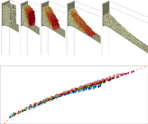
A discrete element simulation of granular column collapses onto an inclined plane of $\theta = 10^{\circ }$. Snapshots are taken at (a) $t = 0$ s, (b) $t = 0.08$ s, (c) $t = 0.12$ s, (d) $t = 0.2$ s and (e) $t = 0.5$ s. The $x$-axis is towards the horizontal direction, and the $z$-axis is towards the vertical direction. Different colours represent different velocity magnitudes of particles. The colour bar in the figure shows the range of colour that corresponds to the velocity magnitude varying from 0 to its maximum.

At the initial condition shown in figure 4(a), we identify the initial domain of the granular column within $L_i \times W_i \times H_i$ and perform the Voronoi tessellation to form a Voronoi granular packing with solid fraction 1. To make sure that granular materials are loosely packed at the initial state, we choose to reduce the initial solid fraction to $\phi _{init} = 0.6$ by randomly removing 40 % of grains from the Voronoi tessellation. The removal of grains has almost no influence on the mean value and standard deviation of the effective particle diameter of the granular system. Then, we release the packing and let it flow onto the incline plane. We set the boundary frictional coefficients on the horizontal plate and on the incline plane at the same value, which is $\mu _w = 0.4$. We also found that a novel null friction boundary could be imposed for reducing computational times proposed by Chung, Kuo & Hsiau (Reference Chung, Kuo and Hsiau2022). However, in this work, we choose a more traditional way to impose frictional conditions since it is consistent with our previous studies (Man et al. Reference Man, Huppert, Li and Galindo-Torres2021a). We also note that, in the simulation work, the boundary condition of imposing merely frictional coefficients is also different from the experimental study of Lube et al. (Reference Lube, Huppert, Sparks and Freundt2011), where the inclined channel was rough and bumpy. Thus, we do not expect our simulation results to be exactly the same as the experimental work of Lube et al. (Reference Lube, Huppert, Sparks and Freundt2011). Figures 4(b)–4(e) show the initiation, propagation and termination of the collapse of a granular column with $H_i = 10$ cm. During the collapse process, we record the translational and angular velocities, positions, translational and rotational kinetic energies and particle interactions of the system. We also measure the front velocity during the collapse and determine the terminal time, $T_f$, based on the magnitude of the front velocity.

After the flow termination, we measure the final horizontal length, $L_{\infty }$, and the deposition height, $H_{\infty }$, of the granular pile, to obtain the parameters shown in figure 1(a). In this work, to quantify the propagation capacity of granular column collapses, we focus on the horizontal relative run-out distance, $\delta L$, instead of the run-out distance along the inclination, $\delta L^{\prime }$. We note that the way we generate the initial packing leads to a much more stable initial state than loosely packed sand. The initial Voronoi-based packing with a initial solid fraction, $\phi _{init}$, is similar to a fissured porous rock. The face-to-face interactions naturally dominate inter-particle contacts at the initial state, which results in a more stable status for the granular packing. This indicates that the scaling results of simulated granular column collapses may be different from the experimental results obtained by Lube et al. (Reference Lube, Huppert, Sparks and Freundt2011), but the underlying physics should be similar. In this work, to investigate the scaling of the run-out behaviour and kinematics of granular column collapses on inclined planes, we set up three different inter-particle frictional coefficients, which are 0.2, 0.4 and 0.6, vary the initial height between 1 and 50 cm, so that the initial aspect ratio, $\alpha = H_i/L_i$, varies from 0.33 to 16.67 and change the inclination angle, $\theta$, from $2.5^{\circ }$ to $20^{\circ }$.

4. Run-out behaviour and flow kinematics

4.1. Horizontal run-out distance

The final run-out distance is a major property for granular column collapses since it exhibits the ability of a granular system to transform potential energy to kinetic energy, and links to propagation capacity and damage level of geophysical flows, such as landslides and pyroclastic flows, in natural systems. Lube et al. (Reference Lube, Huppert, Sparks and Freundt2011) examined the run-out behaviour of granular column collapses on inclined planes and treated the run-out distance on the inclination as a key parameter. However, in this work, we focus on the horizontal run-out behaviour and treat the vertical run-out as a result of both horizontal run-out distance and the inclination angle, and regard the horizontal run-out distance as a direct measurement quantifying the transformation from potential to kinetic energy.

We plot the relative horizontal run-out distance, $\mathcal {L} = (L_{\infty } - L_i)/L_i = \delta L/L_i$, against the initial aspect ratio, $\alpha = H_i/L_i$, of systems with $\phi _{init} = 0.6$ in figure 5(a). For each set of simulations with the same inclination angle $\theta$, we have three different inter-particle frictional properties, i.e. $\mu _p = 0.2$, 0.4 and 0.6. We can see from figure 5(a) that increasing the inter-particle frictional coefficient from 0.2 to 0.6 helps decrease the run-out distance, and changing frictional properties scatters corresponding data points. Increasing the inclination angle greatly increases the run-out distance. For instance, for systems with $\alpha \approx 1.0$ and $\mu _p = 0.4$, $\mathcal {L}$ is less than 1 when $\theta = 2.5^{\circ }$, but $\mathcal {L}$ is already larger than 10 when $\theta = 20^{\circ }$. This indicates that increasing $\theta$ by only a factor of 8 results in a run-out distance more than 10 times longer, which implies that the relationship between the initial aspect ratio and the relative run-out distance is nonlinear.

Figure 5.

Relative horizontal run-out distance of systems with $\phi _{init} = 0.6$ plotted against (a) initial aspect ratio, $\alpha$, (b) effective aspect ratio, $\alpha _{eff}$, and (c) inclined effective aspect ratio, $\tilde {\alpha }_{eff}$, for 21 different sets of simulations. The red curve represents the fitting relationship of $\mathcal {L}\sim \tilde {\alpha }_{eff}^{1.35}$ and the blue curve denotes the fitting of $\mathcal {L}\sim \tilde {\alpha }_{eff}$.

Using the effective aspect ratio $\alpha _{eff}$ that we proposed previously, we are able to collapse the simulation results of systems with the same $\theta$ onto one curve as shown in figure 5(b). We reiterate that the derivation of $\alpha _{eff}$ is based on the assumption that the granular column collapse is governed by the ratio between the inertial effect and the frictional resistance. The ability of $\alpha _{eff}$ to quantify horizontal granular column collapses has been verified in many previous works (Man et al. Reference Man, Huppert, Li and Galindo-Torres2021a, Reference Man, Huppert, Li and Galindo-Torresb, Reference Man, Huppert, Zhang and Galindo-Torres2022, Reference Man, Zhang, Huppert and Galindo-Torres2023), and it still works for a system with an inclined run-out. However, $\alpha _{eff}$ fails to combine all the data into a master curve since the influence of $\theta$ is missing in the definition of it, but most importantly, changing the $x$-axis from $\alpha$ to $\alpha _{eff}$ imposes no effect to the nature that larger inclination angles lead to longer run-out distances. Based on the analysis in § 2, we hypothesize that the inclined effective ratio, $\tilde {\alpha }_{eff}$, which includes both frictional properties and the inclination information, where the calculations of both the inertial effect and the frictional resistance already consider the influence of the inclination angle, could help quantify and unify the relationship between run-out distances and initial geometries.

Figure 5(c) plots the relationship between $\mathcal {L}$ and $\tilde {\alpha }_{eff}$ in a log–log coordinate system for simulation results obtained from granular column collapses with $\theta = 2.5^{\circ }\unicode{x2013}20^{\circ }$. As expected, changing the $x$-axis to $\tilde {\alpha }_{eff}$ helps tremendously, in that almost all the data points fall onto a master curve, except for systems with large $\tilde {\alpha }_{eff}$ and $\theta \leqslant 5^{\circ }$. The $\mathcal {L}\text {-- }\tilde {\alpha }_{eff}$ relationship consists of two parts. When $\tilde {\alpha }_{eff} \lessapprox 4$, $\mathcal {L}$ approximately scales with $\tilde {\alpha }_{eff}^{1.35}$, as shown by the red line in figure 5(b), but when $\tilde {\alpha }_{eff} \gtrapprox 4$, $\mathcal {L}$ approximately scales proportionally to $\tilde {\alpha }_{eff}$, as shown by the blue line in this figure. The parameters of the power-law scaling are different from those in the $\mathcal {L}\unicode{x2013} \alpha _{eff}$ relationship reported by Man et al. (Reference Man, Huppert, Li and Galindo-Torres2021a), since $\tilde {\alpha }_{eff}$ contains information of the final run-out distance $L_{\infty }$ inside its definition. When $\tilde {\alpha }_{eff}\gtrapprox 4$ and $\theta \leqslant 5^{\circ }$, the simulation results slightly deviate from other data points, and the master curve would over-predict the run-out distance. In one of our previous works (Man et al. Reference Man, Huppert, Li and Galindo-Torres2021a), we classified granular column collapses into three different regimes: quasi-static, inertial and fluid-like. One key characteristic of a granular collapse within the fluid-like regime is that the inertial effect becomes so large that the memory of the initial packing, i.e. the initial contact structure and the initial geometry, will be lost, which results in the behaviour that particles initially at the bottom of the packing flow to the very front of the final deposition pile. The data deviation of granular columns with $\tilde {\alpha }_{eff}$ and $\theta \leqslant 5^{\circ }$ implies that the fluid-like regimes for systems with different inclination angles might be different from each other.

We choose two cases to investigate and plot the deposition pattern on the $x\unicode{x2013}z$ plane in figure 6. The red region represent the deposition pattern of a granular column collapse with $\theta = 2.5^{\circ }, \mu _p = 0.4, H_i = 50$ cm, $\tilde {\alpha }_{eff} = 15.94$, and the blue region shows the pattern of a collapse with $\theta = 15^{\circ }, \mu _p = 0.4, H_i = 25$ cm, $\tilde {\alpha }_{eff} = 15.94$. Two systems have similar $\tilde {\alpha }_{eff}$ and both reached the fluid-like regime, as we have argued previously (Man et al. Reference Man, Huppert, Li and Galindo-Torres2021a), but have different inclination angles. The red region shows that, after the granular column collapse, the granular pile is similar to a horizontal granular column collapse with a triangular-like deposition pattern. However, for a granular column collapse with a larger inclination angle, the deposition structure becomes different. The blue region shows that a large part of the deposition is covered by only one or two layers of particles, which indicates a larger relative run-out distance than systems with $\theta = 2.5^{\circ }$ and 5$^{\circ }$. We believe that it is the ability to generate a large area of one-layer particle cover that results in the deviation in the $\mathcal {L}\unicode{x2013}\tilde {\alpha }_{eff}$ plot. In the system represented by the red region, the thin-layered region is small compared with the length of the granular pile. We can find one particle that reaches $X = 80$ cm and a few particles present between $X = 60$ cm and $X = 80$ cm, but those particles are all detached from the main pile and cannot be regarded as a thin-layered area.

Figure 6.

Deposition pattern for granular column collapses with $\theta = 2.5^{\circ }$, $H_i = 50$ cm, $\tilde {\alpha }_{eff} = 15.94$ (as the red region) and $\theta = 15^{\circ }$, $H_i = 25$ cm, $\tilde {\alpha }_{eff} = 15.88$ (as the light blue region).

In summary, with the newly derived inclined effective aspect ratio, $\tilde {\alpha }_{eff}$, we are able to work beyond the experimental results to achieve a good collapse of the data obtained from DEM simulation results with various material properties and initial conditions. Based on the derivation of $\tilde {\alpha }_{eff}$, we believe that $\tilde {\alpha }_{eff}$ represents a ratio between the available inertial effect and the frictional effect, which should govern the transition between different collapsing regimes. Based on this, we further explore the scaling of other parameters, such as the kinetic energy, flow propagation velocities, collapsing duration and deposition heights.

4.2. Kinetic energy

We have found that increasing the inclination angle leads to considerable increase in the run-out distance and results in a longer run-out tail with a thinner layer of particles. In this section, we further explore this behaviour from the viewpoint of the energy transformation. At each time, we record the translational and angular velocity vector of each particle, $\boldsymbol {v}_{p}$ and $\boldsymbol {\varOmega }_{p}$, and calculate its corresponding translational and rotational kinetic energy based on its mass, $m_p$, and its inertia matrix, $\boldsymbol {I}_p$. Then, we quantify the kinetic energy per particle of this system using the following equations:

(4.1a)$$\begin{gather} E_{kt} = N_p^{{-}1}\sum_{p\in N_p}^{N_p}\left(\frac{1}{2} m_p\boldsymbol{v}_p^2 \right) , \end{gather}$$

(4.1b)$$\begin{gather}E_{ka} = N_p^{{-}1}\sum_{p\in N_p}^{N_p}\left(\frac{1}{2} \boldsymbol{I}_{p}\boldsymbol{\varOmega}_{ p}\boldsymbol{\cdot}\boldsymbol{\varOmega}_{p} \right) , \end{gather}$$

where $E_{kt}$ and $E_{ka}$ are translational and rotational kinetic energy per particle, respectively, and $N_p$ is the number of particles in the granular column collapse system. In figures 7(a)–7(c), we plot the time evolution of $E_{kt}$ for granular columns with $\theta = 2.5^{\circ }$, $10^{\circ }$ and $17.5^{\circ }$. We choose systems with five different initial heights to plot. The time evolution of the particle kinetic energy resembles the granular column collapses on a horizontal plane. At the beginning of a collapse, $E_{kt}$ increases nonlinearly with respect to $t$, after which $E_{kt}$ increases rapidly to its peak. Afterwards, the kinetic energy per particle starts to decline. As we increase the initial height from 2 cm to 4 cm, the maximum translational kinetic energy increases, as does the duration of the non-zero $E_{kt}$ period. If we compare systems with different inclination angles, we can see that increasing the inclination angle does not result in much increase in the maximum translational kinetic energy, $E_{kt,max}$. For instance, when $H_i = 40$ cm and $\theta = 2.5^{\circ }$, as shown in figure 7(a), the maximum translational kinetic energy $E_{{kt,max}} \approx 145\ {\rm g}\ {\rm cm}^2\ {\rm s}^{-2}$. As we increase the inclination angle to $10^{\circ }$, $E_{{kt,max}}$ only increases to approximately $155\ {\rm g}\ {\rm cm}^2\ {\rm s}^{-2}$. Further increasing $\theta$ to $17.5^{\circ }$ only manages to increase $E_{{kt,max}}$ to ${\approx }165\ {\rm g}\ {\rm cm}^2\ {\rm s}^{-2}$.

Figure 7.

(a–c) Time evolution of the translational kinetic energy per particle, $E_{kt}$, for systems with $\theta = 2.5^{\circ }$, $\theta = 10^{\circ }$ and $\theta = 17.5^{\circ }$, respectively. We only choose columns with five different initial height ($H_i = 2$ cm, 5 cm, 10 cm, 20 cm and 40 cm) and $\mu _p = 0.4$ to plot. (d–f) Time evolution of the rotational kinetic energy per particle, $E_{ka}$, for systems with $\theta = 2.5^{\circ }$, $\theta = 10^{\circ }$ and $\theta = 17.5^{\circ }$, respectively. We also choose columns with five different initial heights ($H_i = 2$ cm, 5 cm, 10 cm, 20 cm and 40 cm) to plot.

Similar behaviour happens when we analyse the rotational kinetic energy and its maximum for systems with different initial heights and inclination angles, where increasing $\theta$ from $2.5^{\circ }$ to $17.5^{\circ }$ only leads to an increase of $E_{{ka,max}}$ from approximately $38\ {\rm g}\ {\rm cm}^2\ {\rm s}^{-2}$ to $42\ {\rm g}\ {\rm cm}^2\ {\rm s}^{-2}$. This phenomenon may result from the fact that, during a granular column collapse, most of the granular system halts quickly after the release of materials and it is mainly the front part that is propagating, which often results in a long thin layer of particles, as shown in figure 6. Additionally, this behaviour implies that the major influence of the inclination angle is to extend the collapse duration rather than to increase $E_{{kt,max}}$ or $E_{{ka,max}}$.

We normalize both the per particle maximum translational and rotational kinetic energies using $\langle m_p\rangle gH_i$, where $\langle m_p\rangle \approx 0.0221$ g is the average particle mass, and plot them in figure 8. Figure 8(a) shows on a logarithmic coordinate system the relationship between the dimensionless maximum particle kinetic energy, $\mathcal {E}_{{kt,max}} = E_{ kt,max}/(\langle m_p\rangle gH_i)$, and the effective aspect ratio, $\alpha _{eff}$. The $\mathcal {E}_{{kt,max}}\unicode{x2013} \alpha _{eff}$ relation seems to collapse well, which confirms that changing the inclination angle has almost no influence on the maximum kinetic energy, $E_{kt,max}$, during the granular column collapse. We note that, in figure 8(a), the $x$-axis is $\alpha _{eff} = \alpha \sqrt {1/(\mu _w + \beta \mu _p)}$, which bears no $\theta$-related influences. As we increase $\alpha _{eff}$, $\mathcal {E}_{{kt,max}}$ gradually converges to a power-law relationship that scales with $\alpha _{eff}$. The convergence point $\alpha _{eff}\approx 2$ coincides with turning points in the $\mathcal {L}\unicode{x2013}\alpha _{eff}$ relationships shown in figure 5(b), where slopes change at $\alpha _{eff}\approx 2$ for almost all sets of simulations with different inclination angles. Figure 8(b) shows the failure of $\tilde {\alpha }_{eff}$ in terms of collapsing data of $\mathcal {E}_{kt,max}$. It confirms that changing the inclination angle does not greatly affect the maximum translational kinetic energy a granular system can achieve during column collapses.

Figure 8.

(a) Relationship between the dimensionless maximum translational kinetic energy per particle in each simulation, $E_{{kt,max}}/(\langle m_p\rangle gH_i)$, and $\alpha _{eff}$. (b) Relationship between $E_{{kt,max}}/(\langle m_p\rangle gH_i)$ and $\tilde {\alpha }_{eff}$. (c) Relationship between the dimensionless maximum rotational kinetic energy per particle in each simulation, $E_{{ka,max}}/(\langle m_p\rangle gH_i)$, and $\alpha _{eff}$. (d) Relationship between $E_{{ka,max}}/(\langle m_p\rangle gH_i)$ and $\tilde {\alpha }_{eff}$. The kinetic energies are normalized using $\langle m_p\rangle gH_i$, where $\langle m_p\rangle \approx 0.0221$ g is the average particle mass. Markers in this figure are the same as those in figure 5.

Figures 8(c) and 8(d) show relationships of $\mathcal {E}_{ka,max}\unicode{x2013}\alpha _{eff}$ and $\mathcal {E}_{ka,max}\unicode{x2013}\tilde {\alpha} _{eff}$, respectively. Despite the scatter of the $E_{ka,max}\unicode{x2013}\tilde {\alpha }_{eff}$ relationship, the $E_{ka,max}\unicode{x2013}{\alpha }_{eff}$ relationship collapses well onto a master curve, where the $E_{ka,max}$ gradually converges to a linear curve as we increase ${\alpha }_{eff}$. We can also determine which kinetic energy is dominating the collapse process from figures 8(a) and 8(c). When $\alpha _{eff} \approx 0.3$, $\mathcal {E}_{kt,max}$ is between 0.005 and 0.008, while $\mathcal {E}_{ka,max}$ is approximately 0.018. This indicates that, when $\alpha _{eff}$ is small, most of the potential energy will be transformed into rotational kinetic energy. This corresponds to the quasi-static collapse illustrated by Man et al. (Reference Man, Huppert, Li and Galindo-Torres2021a), where the granular column slumps like a viscous solid and particles often roll down the granular slope, since the effective shear rate and its corresponding stress are not large enough to overcome the frictional interaction between contacting pairs. When $\alpha _{eff} \approx 2$, $E_{kt,max}$ and $E_{ka,max}$ become almost equal, after which the translational kinetic energy dominates in the collapse process. The plots in figures 8(c) and 8(d) also show that when $\alpha _{eff}\gtrapprox 2$ or $\tilde {\alpha }_{eff}\gtrapprox 3$, the normalized $E_{{ka,max}}$ remains almost constant. This transitional point also demonstrates the transition where the translational kinetic energy starts to dominate the collapsing process.

We note that the behaviour of the maximum kinetic energy achieved during granular column collapses does not scale well with the newly proposed $\tilde {\alpha }_{eff}$, which should not be interpreted as a disadvantage of $\tilde {\alpha }_{eff}$. In contrast, it indicates that $\tilde {\alpha }_{eff}$ can do a better job to describe variables that are related to the whole collapsing process. Here, $\mathcal {E}_{kt,max}$ and $\mathcal {E}_{ka,max}$ are more related to the failure and collapse initiation of the granular column than to the energy dissipation process that occurs dominantly on the inclined slope. This is the reason why $\alpha _{eff}$ performs better in terms of describing the maximum kinetic energies.

4.3. Maximum propagation velocity

The maximum kinetic energy measures the average capacity of the whole system to transform the potential energy into kinetic energy. If we regard a granular column collapse as a potential small-scale landslide, we should also investigate its front velocity, $u_{fr}$, since it directly links to the damage that a real slope collapse can cause to people and structures. For a granular column and at each time step, we select a few particles located at the front and calculate their average velocity as the front velocity of this granular system. We note that the front position, for most of the simulations, is determined by the farthest particle, and the front velocity is calculated by averaging velocities of particles both at and close to the front position with a range of a certain length scale. For example, if the $x$-coordinate of the front is $x_f$, we calculate the front velocity by averaging velocities of particles within $(x_f-5d_{ep}, x_f)$. We also note that, for a few simulations, one or two particles may run ahead of all other particles with a great distance due to some random collision with a large contact force. Even though these kinds of particles are the farthest, we do not consider them as the front position because these particles are already detached from the main granular flow.

We plot the time evolution of $u_{fr}$ for systems with $\theta = 2.5^{\circ }, 10^{\circ }$ and $17.5^{\circ }$ in figure 9. Similar to figure 7, we only choose cases with $H_i =2$ cm, 5 cm, 10 cm, 20 cm and 40 cm to plot. Compared with figure 7, we notice that the duration of $u_{fr}$ is usually longer than that of the kinetic energy, especially when the initial aspect ratio is large. For instance, for granular systems with $\theta = 2.5^{\circ }$ and $H_i = 40$ cm, $u_{fr}$ decays to 0 at $t \approx 0.75$ s, while $E_{kt}$ declines to almost 0 before $t = 0.6$ s and $E_{ka}$ decreases to approximately 0 at $t \approx 0.65$ s. This is due to both $E_{kt}$ and $E_{ka}$ being averages of the whole granular system. After a granular system reaches its peak kinetic energy, most particles that are lagging behind stop moving, while only front particles continue to propagate, which results in a longer duration for $u_{fr}$ than for the kinetic energy.

Figure 9.

Time evolution of the front velocity for granular columns with (a) $\theta = 2.5^{\circ }$, (b) $\theta = 10^{\circ }$ and (c) $\theta = 17.5^{\circ }$. We set $\mu _p = 0.4$ in all three sets of simulation results.

Figure 9 shows that the decay of the front velocity is approximately linear, which is different from the decay of the kinetic energy. Additionally, the linearity becomes more obvious when we tune the granular column to be taller and the inclined plane to be steeper. Both the initial aspect ratio and the inclination angle play important roles in determining the maximum front velocity and the collapse duration. In figure 7, when $\theta = 2.5$ and $H_i = 10$ cm, the maximum front velocity is $u_{fr,max}\approx 128.8\ {\rm cm}\ {\rm s}^{-1}$ at $T_{ufr,max} = 0.16$ s, and the front velocity lasts for 0.45 s. As we increase the inclination to $10^{\circ }$, $u_{fr,max}$ only grows by 11 % and $T_{ufr,max}$ by 25 %, but the front velocity duration is increased by 57.8 %. Similar measurements occur when we increase the inclination angle from $10^{\circ }$ to $17.5^{\circ }$, while $u_{fr,max}$, $T_{ufr,max}$ and the front velocity duration increase by 9.9 %, 50 % and 136.6 %, respectively. If we examine the results for systems with $H_i = 40$ cm, we can find similar behaviours. Then, we conclude that changing the inclination angle plays a more important role in determining the time-related information than that in quantifying the maximum front velocity. In other words, if a granular column collapse is considered as a landslide or a volcano-induced pyroclastic flow, a larger slope angle may not result in a heavier damage since the front velocity does not change much, it can certainly influence larger areas since the collapse duration is increased considerably. Meanwhile, comparing figure 9 with figure 7 shows that the maximum front velocity always comes later than the maximum kinetic energy, which indicates that the front particles are still accelerating, while the majority of the particles already start to decelerate. This implies that, slightly different from the kinetic energy, it is possible that both $\alpha _{eff}$ and $\tilde {\alpha }_{eff}$ play important roles in describing the front velocity.

We normalize the maximum front velocity, $u_{fr,max}$, with a characteristic velocity scale, $\sqrt {gH_i}$, and plot it against ${\alpha }_{eff}$ and $\tilde {\alpha }_{eff}$ in figure 10. The relationship between $u_{fr,max}$ and $\alpha _{eff}$ in figure 10(a) shows that, as we increase $\alpha _{eff}$ from 0.3 to ${\approx }2.0$, the normalized maximum front velocity increases accordingly, whereas $u_{fr,max}/\sqrt {gH_i}$ starts to decrease as we further increase $\alpha _{eff}$ afterwards. Meanwhile, when the inclination angle is large, there is seemingly a plateau for $u_{fr,max}/\sqrt {gH_i}$ within $\alpha _{eff}\in (1.0, 4.0)$. The figure for the $u_{fr,max}/\sqrt {gH_i}\sim \tilde {\alpha }_{eff}$ relationship shown in figure 10(b) brings up more interesting results. As we increase $\tilde {\alpha }_{eff}$, the $u_{fr,max}/\sqrt {gH_i}\sim \tilde {\alpha }_{eff}$ relation exhibits two ascending paths (red and blue solid lines) and descending paths (red and blue dashed lines) that depends on both the inclination angle and the frictional properties. When $\tilde {\alpha }_{eff}\lessapprox 2.0$, $u_{fr,max}/\sqrt {gH_i}$ scales with $\tilde {\alpha }_{eff}^{0.5}$ as denoted by the red solid line. Afterwards, the ascending slope decreases from 0.5 to ${\approx }0.1$. The second ascending path is followed by a descending path, but the descending paths for systems with different inclination angles and different frictional properties tend to be quite different from each other, as shown by the red and blue dashed lines in figure 10(b). For example, when the inclination angle is $\theta =2.5^{\circ }$, $u_{fr,max}/\sqrt {gH_i}$ starts to decrease after $\tilde {\alpha }_{eff}\gtrapprox 4$ and scales with $\tilde {\alpha }_{eff}^{-0.5}$. When the inclination angle is $\theta =2.5^{\circ }$ and the frictional coefficient is small, $u_{fr,max}/\sqrt {gH_i}$ starts to decrease after $\tilde {\alpha }_{eff}\gtrapprox 30$ and scales with $\tilde {\alpha }_{eff}^{-0.25}$.

Figure 10.

(a) Relationship between the maximum front velocity, $u_{fr,max}$, and $\alpha _{eff}$. (b) Relationship between the maximum front velocity, $u_{fr,max}$, and $\tilde {\alpha }_{eff}$. The red solid line scales with $\tilde {\alpha }_{eff}^{0.5}$ and the blue solid line scales with $\tilde {\alpha }_{eff}^{0.1}$. The red dashed line scales with $\tilde {\alpha }_{eff}^{-0.25}$ and the blue dashed line scales with $\tilde {\alpha }_{eff}^{-0.5}$. Markers in this figure are the same as those in figure 5.

4.4. Collapse duration

We further investigate how much time it takes for a granular column collapse to come to rest, which is the collapse duration. For granular columns with the same initial aspect ratio, as we increase the inclination angle, the run-out distance will also increase, which may result in a longer propagation period and a larger value of the terminal time, $T_f$. In this work, we define $T_f$ based on the time evolution of the front velocity and regard the time when the front velocity diminishes as the terminal time for the collapse. Both Lube et al. (Reference Lube, Huppert, Sparks and Hallworth2004) and Lube et al. (Reference Lube, Huppert, Sparks and Freundt2005) stated that, based on dimensional analysis, $T_f$ must scale with $(L_i/g)^{0.5}\psi (\alpha )$, where $\psi (\alpha )$ is a function of the initial aspect ratio. Man et al. (Reference Man, Zhang, Huppert and Galindo-Torres2023) then concluded that, for systems with different frictional coefficients, $\psi (\alpha )$ should be modified to $\psi (\alpha _{eff})$ and argued that $\psi (\alpha _{eff}) = \kappa _t\alpha _{eff}^{0.5}$, where $\kappa _t$ is a constant, is the best fit to the simulation results. However, the duration of a granular column collapse should be more related to the initial height of the system. Thus, Lube et al. (Reference Lube, Huppert, Sparks and Freundt2011) hypothesized the scaling of $T_f$ to be $T_f \propto \sqrt {H_i/g}$. Because column collapses on inclined planes will inevitably introduce additional potential energy (comparing to granular column collapses on horizontal planes) to be transferred into kinetic energy, we believe that this will introduce an additional length scale to the scaling of $T_f$. Thus, we express $T_f$ as

(4.2)\begin{equation} T_f = \psi(\tilde{\alpha}_{eff})\left[(H_i + \delta L\tan{\theta})/a_c\right]^{1/2} , \end{equation}

where $a_c$ is an acceleration scale, which can be written as $a_c = g/\mathcal {A}_{th}^2$. As we change the inclination angle, the acceleration scale of $T_f$ should also be changed, which will introduce a function of $\theta$ as a factor of $g$. Then, we can define the dimensionless collapse duration $\mathcal {T}_f$ as

(4.3)\begin{equation} \mathcal{T}_{f} \equiv T_f\left[(H_i + \delta L\tan{\theta})/g\right]^{{-}1/2} = \mathcal{A}_{th}(\theta)\psi(\tilde{\alpha}_{eff}). \end{equation}

Based on (4.3), we plot the relationship between $\mathcal {T}_f/\mathcal {A}_{th}(\theta )$ and $\tilde {\alpha }_{eff}$ in figure 11. Here, $\mathcal {A}_{th}$ is a function of $\theta$, so we fit (4.3) so that all the simulation data collapse onto one master curve, which can be expressed as

(4.4)\begin{equation} \mathcal{A}_{th} = A_o + \epsilon_1 \cdot \exp\left[ \varTheta_f/(s_t-\tan\theta) \right],\quad \tan\theta\leqslant s_t , \end{equation}

where $A_o \approx 4.111$, $\epsilon _1\approx 4.1\times 10^{-3}$, $\varTheta _f \approx 4.59$ and $s_t \approx 0.94$ are fitted parameters. The R-squared of the fitting curve is approximately 0.9998. This equation indicates that, when $\tan \theta$ is approaching $s_t$, $\mathcal {A}_{tf}$ is inevitably reaching infinity. We note that, in this work, the frictional coefficient between the inclined plane and particles is $\mu _w = 0.4$, yet the fitted $s_t$ is much larger than $\mu _w$, which implies that an inclined plane with slope larger than $\arctan (\mu _w)$ can still hold Voronoi-based grains. This may be because Voronoi-based particles innately have rolling resistances due to their random, non-spherical, angular shapes. Figure 11 shows that $\psi (\tilde {\alpha }_{eff})$ follows a power-law function of $\tilde {\alpha }_{eff}$, where the exponent is approximately $-0.066$ and the relationship can be expressed as

(4.5a,b)\begin{equation} \psi(\tilde{\alpha}_{eff}) = \tilde{\alpha}_{eff}^{\zeta},\quad \zeta \approx{-}0.066 . \end{equation}

Figure 11.

Relationship between the dimensionless collapse duration, $\mathcal {T}_f \equiv T_f/\sqrt {(H_i+\delta L\tan {\theta })/g}$, and $\tilde {\alpha }_{eff}$. The fitting curve follows a power-law relation with $\mathcal {T}_{f} = \mathcal {A}_{th}\cdot \tilde {\alpha }_{eff}^{\zeta }$, where $\zeta$ is a fitted parameter and $\mathcal {A}_{th}$ can be calculated based on $\theta$, which is plotted in the inset of this figure. Markers in this figure are the same as those in figure 5.

We can see that $\zeta$ is a small number, which indicates that the collapse duration is only weakly influenced by the scaling variable $\tilde {\alpha }_{eff}$, but strongly dependent on the time scale of $\sqrt {(H_i+\delta L\tan {\theta })/g}$. Nevertheless, $\tilde {\alpha }_{eff}$ can help unify the influence of both the frictional contacts among particles and the inclination angles and the previously proposed effective aspect ratio, $\alpha _{eff}$, would make this relationship more scattered.

5. Final deposition height

For granular column collapses, longer run-out distances often result in shorter final deposition heights, $H_{\infty }$. In a previous study (Man et al. Reference Man, Zhang, Huppert and Galindo-Torres2023), we showed the complexity of the relationship between $H_{\infty }$ and $\alpha _{eff}$ for systems with different inter-particle frictional properties. However, the complexity was somewhat overcome as we, instead of focusing only on $H_{\infty }$, analysed the volume of the deposition cone, $\mathcal {V}_{cone}$, and the ratio between $\mathcal {V}_{cone}$ and the initial column volume $\mathcal {V}_{init}$. In this work, we first investigate the relationship between $H_{\infty }/L_i$ and dimensionless numbers, as shown in figures 12(a)–12(c), to show how the deposition height scales with different scaling variables. We note that the deposition height often measures the amount of granular materials that remains static during the column collapse. Thus, we suspect that the scaling of $H_{\infty }$ is mainly influenced by the aspect ratio and the frictional properties, and the inclination angle may only play a minor role, which might be quite different for the scaling of the run-out distance.

Figure 12.

(a–c) Relationships between $H_{\infty }/L_i$ and $\alpha$, $\alpha _{eff}$ and $\tilde {\alpha }_{eff}$, respectively. (d) Relationship between $H_{\infty }/\delta L$ and $\alpha _{eff}$. (e) Relationship between $H_{\infty }/H_i$ and $\alpha _{eff}$. (f) Rescaled dimensionless deposition height, $\mathcal {A}_{th}(\theta )\hat {H}_{\infty }/H_i$ against $\alpha _{eff}$. Markers are the same as those in figure 5.

The relationship between $H_{\infty }/L_i$ and $\alpha$ exhibits power-law characteristics of $H_{\infty }/L_i\sim \alpha ^{\xi }$, as shown in figure 12(a). For granular columns with the same frictional property and the same inclination angle but different initial column heights, when $\alpha$ is below a threshold $\alpha _{hc}$, $H_{\infty }/L_i$ always scales with $\alpha$ and $\xi = 1$ (the green line in figure 12a), but when $\alpha$ is larger than a threshold $\alpha _{hc}$, $H_{\infty }/L_i$ scales with $\alpha ^{\xi }$ and $\xi$ is much smaller than 1. When $\alpha >\alpha _{hc}$, as we increase the inclination angle from 2.5$^{\circ }$ to 20$^{\circ }$ and the inter-particle frictional coefficient from 0.6 to 0.2, the power-law exponent, $\xi$, decreases from ${\approx }1/3.5$ to ${\approx }1/20$, which indicates that it is difficult for granular columns with larger inclination angles to sustain a larger deposition height because particles tend to flow further on planes with larger $\theta$. We note that the transition point, $\alpha _{hc}$, varies with respect to both the inclination angle and the frictional properties. As we change the inclination angle from 2.5$^{\circ }$ to 20$^{\circ }$ and the inter-particle frictional coefficient from 0.6 to 0.2, $\alpha _{hc}$ varies from ${\approx }0.6$ to 1.0. As expected and similar to our previous study (Man et al. Reference Man, Zhang, Huppert and Galindo-Torres2023), changing the $x$-axis from $\alpha$ to $\alpha _{eff}$ or $\tilde {\alpha }_{eff}$ (figure 12b,c), instead of solving the discreteness of simulation data, further increases the pronounced scattering, which leads us to combine deposition height with the run-out behaviour and to introduce a different length scale to non-dimensionalize the deposition height.

Plotting the ratio between $H_{\infty }$ and $\delta L$ against $\alpha _{eff}$ in figure 12(d) helps unify the influence of frictional properties. The $H_{\infty }/\delta L\sim \alpha _{eff}$ relationship of systems with different frictional coefficients, but the same inclination angle, seems to collapse onto one master curve. However, the most straightforward way to normalize $H_{\infty }$ is to divide it by its initial column height. As we plot the relationship between $H_{\infty }/H_i$ and $\alpha _{eff}$, the simulation results can be divided into two parts. When $\alpha _{eff}\lessapprox 1.0$, $H_{\infty }/H_i$ is constant and equal to 1.0. However, when $\alpha _{eff}\gtrapprox 1.0$, the $H_{\infty }/H_i\sim \alpha _{eff}$ relationship tends to collapse onto a power-law function, and the exponent of this power-law function varies with the change of the inclination angle. As we increase the inclination angle, $H_{\infty }/H_i$ decays faster with the increase of $\alpha _{eff}$.

Learning from Lube et al. (Reference Lube, Huppert, Sparks and Freundt2011), when $\alpha _{eff}\gtrapprox 1.0$, we can express the deposition height, $H_{\infty }$, as the following function:

(5.1)\begin{equation} H_{\infty} = H_i\varphi_{H}\left(\alpha_{eff}, \theta\right), \end{equation}

where $\varphi _H$ is a dimensionless function of $\alpha _{eff}$ and $\theta$. Figure 12(e) shows that changing $\theta$ leads to the change of the power-law exponent, so that $\varphi _H$ follows a functional form of $\alpha _{eff}^{F_H(\theta )}$. However, as we re-scale the deposition height by subtracting an inclination height, $L_i\tan {\theta }$, the exponents of the power-law relationship tend to collapse onto the same value, but this re-scaling inevitably introduces another factor of $\theta$ in the equation, which can be expressed as

(5.2)\begin{equation} \hat{H}_{\infty} \equiv H_{\infty}-L_i\tan{\theta} = H_i\alpha_{eff}^{\eta}\mathcal{F}_H(\theta) , \end{equation}

where $\eta \approx -0.9$ is the unified power-law factor and $\mathcal {F}_H(\theta )$ is the additional dimensionless function of $\theta$. Since increasing $\theta$ leads to the decrease of $\hat {H}_{\infty }$, we hypothesize that $\mathcal {F}_H = 1/\mathcal {A}_{th}$, where $\mathcal {A}_{th}$ is exactly the same as that shown in (4.4). In figure 12(f), we plot the relationship between $\mathcal {A}_{th}(\theta )\hat {H}_{\infty }/H_i$ and $\alpha _{eff}$ and find that, when $\alpha _{eff}>1.0$, the simulation results follow a unified power-law decay. The scaling of the deposition height can be expressed as

(5.3) \begin{equation} H_{\infty} \approx \left\{\begin{array}{@{}ll} H_i, & \alpha_{eff} \leqslant 1.0, \\ {}[k_h/\mathcal{A}_{th}(\theta)]H_i\alpha_{eff}^{\eta} + L_i\tan{\theta}, & \alpha_{eff} > 1.0, \end{array} \right. \end{equation}

where $k_h$ is a fitted factor, which may also be a function of the initial solid fraction of the granular column, which often influences the stability and yielding behaviour of the granular column collapses, as we will further analyse in the next section.

6. Influence of initial solid fractions

The phenomena listed in previous sections are acquired from our study of granular systems with $\phi _{init} = 0.6$. However, the initial solid fraction often plays an important role in determining the macroscopic behaviour of granular flows, especially for systems in subaqueous environments (Pailha, Nicolas & Pouliquen Reference Pailha, Nicolas and Pouliquen2008). Even for dry granular systems, changing the initial solid fraction can evidently affect the dynamical behaviour (Man et al. Reference Man, Zhang, Huppert and Galindo-Torres2023). Thus, we perform another set of simulations for granular column collapses with $\phi _{init} = 0.8$ and investigate how changing the initial solid fraction influences the run-out behaviour, the collapse duration and the deposition height. With the change of the initial solid fraction, we are able to show that the choice of $\tilde {\alpha }_{eff}$ also works for systems with different initial solid fractions. We expect that, for granular columns with larger initial solid fractions, the column collapse may result in a dilation process due to the shearing effect, which can lead to a longer run-out distance.

In figure 13, we plot relationships between $\mathcal {L}$ and $\alpha$, $\alpha _{eff}$ and $\tilde {\alpha }_{eff}$. In contrast to our expectation that increasing the solid fraction leads to pronouncedly larger $\mathcal {L}$, simulation results for systems with $\phi _{init}=0.8$ do not differ much from those for systems with $\phi _{init} = 0.6$. We note that, when we plot $\mathcal {L}$ against $\tilde {\alpha }_{eff}$ in figure 13(c), the simulation data collapse better than for those of systems with $\phi _{init} = 0.6$. The only difference between the two plots shown in figures 5 and 13, brought about by raising $\phi _{init}$ from 0.6 to 0.8, is that, when $\tilde {\alpha }_{eff}>10$ and $\theta \leqslant 5^{\circ }$, the run-out distance of systems with $\phi _{init} = 0.8$ is larger than that of systems with $\phi _{init} = 0.6$. This leads us to the conclusion that, for dry granular columns with initially stable structures, the initial solid fraction is less significant compared with other parameters.

Figure 13.

Relative horizontal run-out distance of systems with $\phi _{init} = 0.8$ plotted against (a) initial aspect ratio, $\alpha$, (b) effective aspect ratio, $\alpha _{eff}$, and (c) inclined effective aspect ratio, $\tilde {\alpha }_{eff}$, for 21 different sets of simulations. The red curve represents the fitted relationship of $\mathcal {L}\sim \tilde {\alpha }_{eff}^{1.35}$ and the blue curve denotes the fitting of $\mathcal {L}\sim \tilde {\alpha }_{eff}$.

Based on the influence of the initial solid fraction on the run-out behaviour of granular column collapses on inclined planes, we can expect that the collapse duration, $T_f$, of systems with $\phi _{init}=0.8$ behaves similarly to that of granular columns with $\phi _{init}=0.6$. Similar to the behaviour of the run-out distance, as we plot in figure 14(a), the relationship between $\mathcal {T}_f/\mathcal {A}_{th}(\theta )$ and $\tilde {\alpha }_{eff}$ of systems with $\phi _{init} = 0.8$ along with the simulation results with $\phi _{init} = 0.6$ agree with each other well, without introducing new factors of the initial solid fraction, and the final scaling of the collapse duration reads $T_f \approx \mathcal {A}_{th}(\theta )\tilde {\alpha }_{eff}^{-0.066}\sqrt {(H_i+\delta L\tan {\theta })/g}$. This indicates that, as long as the initial granular packing is stable under self-weight, changing the initial solid fraction has no influence on the collapse duration. However, the initial solid fraction does play an important role in the final deposition height of a collapsed granular column because the initial packing structure influences the initial stability and the initial failure criterion of granular columns. Consequently, larger initial solid fractions often indicate that fewer particles participate in the granular avalanche and leads to a higher final deposition height.

Figure 14.

(a) Relationship between $\mathcal {T}_f/\mathcal {A}_{th}(\theta )$ and $\tilde {\alpha }_{eff}$ for granular columns with initial solid fraction of both $\phi _{init} = 0.6$ and $\phi _{init} = 0.8$, where $\mathcal {A}_{th}$ is calculated with (4.4). (b) Relationship between $\mathcal {A}_{th}(\theta )\hat {H}_{\infty }/H_i$ and $\alpha _{eff}$ for granular column collapses with $\phi _{init} = 0.6$ and $\phi _{init} = 0.8$. (c) Collapse of all the simulation data once we rescale the $y$-axis of panel (b) with a factor of $\phi _{init}^2$. Markers are the same as those in figures 5 and 13.

To examine the feasibility of (5.3) granular columns with $\phi _{init} = 0.8$, we plot the relationship between $\mathcal {A}_{th}(\theta )\hat {H}_{\infty }/H_i$ and $\alpha _{eff}$ in figure 14(b), where $\mathcal {A}_{th}(\theta )$ is calculated using (4.4) and is exactly the same as the re-scaling factor for the collapse duration. With the renormalization of $\mathcal {A}_{th}(\theta )$, all the simulation data with the same initial solid fraction collapse onto one master curve, but this master curve varies as we change the initial solid fraction $\phi _{init}$ from 0.6 to 0.8.

Figure 14(b) shows that granular columns with larger $\phi _{init}$ tend to sustain taller final deposition heights than systems with small initial solid fractions. We hypothesize that the change of the $\mathcal {A}_{th}(\theta )\hat {H}_{\infty }/H_i\sim \alpha _{eff}$ relationship results from the $\phi _{init}$-induced change of the yielding behaviour of the granular packing. We realize that changing the initial solid fraction does not much affect the universality of the dimensionless numbers we proposed and modify the scaling function of $\mathcal {A}_{th}$, but will influence the magnitude of the deposition heights. This is because increasing the initial solid fraction enhances the initial stability of the granular system, which will prevent more particles from running out and will eventually lead to a relatively larger deposition heights. Meanwhile, sheared granular systems with larger initial solid fractions may also experience the shearing dilation, which can also increase the deposition height of the system. We realize that changing the initial solid fraction has more influence on the deposition height than on the run-out behaviour, and suspect that the initial structure also has more influence on the deposition height. Also, the reason why the deposition height scales better with $\alpha _{eff}$ may be because of the specific boundary we choose, where the initial granular column sits on a horizontal plane, instead of sitting on an inclined plane. It will be the particles, which remain on this horizontal plane after the column collapse, that determine how tall the final deposition should be.

In retrospect, we hypothesize that, when $\alpha _{eff}>1.0$, the factor $k_h$ in (5.3) is dependent on the initial solid fraction of the granular column; and the behaviour in figure 14(b) agrees with this hypothesis. In figure 14(c), we re-scale the $y$-axis with a factor of $\phi _{init}^2$. It shows that the relationship between $\mathcal {A}_{th}(\theta )\hat {H}_{\infty }/(\phi _{init}^2H_i)$ and $\alpha _{eff}$ for all sets of simulations collapse onto one master curve, where $\mathcal {A}_{th}(\theta )\hat {H}_{\infty }/(\phi _{init}^2H_i)$ scales with $\alpha _{eff}^{\eta }$ and $\eta \approx -0.9$. So, when $\alpha _{eff}>1.0$, the scaling of $H_{\infty }$ can be written as $H_{\infty } = [\kappa _h\phi _{init}^2/{\mathcal {A}_{th}(\theta )}]H_i\alpha _{eff}^{\eta } + L_i\tan {\theta }$, where $\kappa _h \approx 15$ is a fitting parameter. This implies that the variable, $k_h$, in (5.3) is indeed a function of the initial solid fraction and can be expressed as $k_h = \kappa _h\phi _{init}^2$.

7. Further discussions

In previous sections, we showed that by considering the extra energy input due to the inclination, the proposal of the inclined aspect ratio, $\tilde {\alpha }_{eff}$, works well in terms of describing the relative run-out behaviour of granular column collapses on inclined planes. Meanwhile, although we obtain a fair collapse of time-related variables, we have also shown the difficulties in obtaining universal descriptions for variables, such as translational and rotational kinetic energies and the maximum front velocity. Most importantly, with $\theta$, $\alpha _{eff}$ and $\tilde {\alpha }_{eff}$, we are able to provide functional forms to determine the deposition height and the collapse duration of granular column collapses on inclined planes with fair accuracy. However, further discussion related to the run-out distance is still needed, because the two-stage power-law relationship between $\mathcal {L}$ and $\tilde {\alpha }_{eff}$ is not completely promising and the transitional point between the two power-law relationships is unclear and equivocal. In figures 5(c) and 13(c), we fit the relationship with two power-law relations, and these fittings work well. However, a two-stage power-law relationship implies a sharp slope change in the plot, and after taking away the two fitting power-law curves, we think that the transition is not sharp enough. It seems that, as we continue increasing $\tilde {\alpha }_{eff}$, the $\mathcal {L} \sim \tilde {\alpha }_{eff}$ relationship will indeed approach an asymptotic power-law solution, but the whole curve is not a two-stage power-law relation with a sharp transition any more.

To resolve our concerns with the $\mathcal {L} \unicode{x2013}\tilde {\alpha }_{eff}$ relationship, we regard the evolution of $\mathcal {L}$ with $\tilde {\alpha }_{eff}$ as a phase transition process, where granular collapses transform from quasi-static regimes to fluid-like regimes (Man et al. Reference Man, Huppert, Li and Galindo-Torres2021a). When the granular column is in a fluid-like regime, we hypothesize that the $\mathcal {L} \unicode{x2013} \tilde {\alpha }_{eff}$ relationship will reach a power-law asymptote. This results in a exponential-type equation

(7.1)\begin{equation} \mathcal{L} = \kappa\tilde{\alpha}_{eff}\exp\left[ - \mathcal{E}/(\tilde{\alpha}_{eff} - \alpha_{one})^{\beta} \right], \end{equation}

where $\kappa = 2.5$, $\mathcal {E} = 0.4$ and $\beta = 0.8$ are fitting parameters, and $\alpha _{one}$ can be seen as the initial aspect ratio for granular columns with only one layer of particles, so that $\alpha _{one} = d_{ep}/L_i$. The introduction of $\alpha _{one} = d_{ep}/L_i$, which may not be exact, ensures reasonably that $\mathcal {L}$ will approach 0 when $\tilde {\alpha }_{eff}$ is small enough. We combine the data in figures 5 and 13, and plot them in figure 15(a). We plot (7.1) as the dashed curve in figure 15(a). It shows that the simulation data agree extremely well with the proposed (7.1). Further analyses are still needed to validate the exponential-type equation and to find physical interpretations for parameters in (7.1).

Figure 15.

(a) Relationship between $\mathcal {L}$ and $\tilde {\alpha }_{eff}$ of granular columns with both $\phi _{init} = 0.6$ and $\phi _{init} = 0.8$. Markers are the same as those in figures 5 and 13. (b) With the time scale we proposed in (2.2), we introduce a new way to normalize the collapse duration that $\mathcal {T}_{new} \equiv T_f/[(H_i+\delta h)/\sqrt {gH_i}]$, and plot the relationship between $\mathcal {T}_{new}$ and $\tilde {\alpha }_{eff}$ in panel (b).

Also, we performed four additional sets of simulations with large particle restitution coefficients to clarify the possible ‘cohesive’ effect that may influence the macroscopic behaviours. We choose systems with inclination angles of $\theta = 5^{\circ }$, $10^{\circ }$ and $15^{\circ }$, and set their restitution coefficient to be $e_n = 0.9$. For systems with $\theta = 10^{\circ }$, we also perform another set of simulations with $e_n = 0.5$. We measure their run-out distance, calculate both $\mathcal {L}$ and $\tilde {\alpha }_{eff}$, and plot their $\mathcal {L}\sim \tilde {\alpha }_{eff}$ relationships as pentagrams in figure 15(a). The results show that changing the restitution coefficient does not result in different scaling patterns of the normalized run-out distance. Since the inclination angle is sufficiently small, the granular system is still considered as a densely packed system, where the restitution coefficient does not greatly influence the system. We understand that the study on the influence of restitution coefficient is not thorough enough. Our granular system may happen to be within a regime that the macroscopic behaviour is insensitive to the change of collisional energy dissipations, but relatively sensitive to the change of frictional contacts. We are determined to further this study in future works.

What concerns us the most is the additional function of the inclination angle, $\mathcal {A}_{th}(\theta )$, when we analyse the scaling of the collapse duration. In § 4.4, we normalize $T_f$ with $\sqrt {(H_i+\delta h)/a_c}$, which is straightforward and is similar to the widely accepted time scale, $\sqrt {H_i/g}$ (Lube et al. Reference Lube, Huppert, Sparks and Freundt2011). However, since $a_c$ is related to the inclination angle, an additional function of $\theta$ is naturally introduced. One of the reviewers reminded us that we defined another characteristic time scale in § 2, where the time is normalized by $(H_i+\delta h)/\sqrt {gH_i}$, with $H_i + \delta h$ a characteristic length and $\sqrt {gH_i}$ a characteristic velocity. It seems that this new time scale may eliminate the additional function of $\theta$ that worries us. Thus, we calculate the new dimensionless collapse duration,

(7.2)\begin{equation} \mathcal{T}_{new} \equiv T_f/[(H_i+\delta L\tan{\theta})/\sqrt{gH_i}]. \end{equation}

In figure 15(b), we plot the relationship between $\mathcal {T}_{new}$ and $\tilde {\alpha }_{eff}$ for simulations with both $\phi _{init} = 0.6$ and $\phi _{init} = 0.8$. It shows that all the simulation results collapse well onto a master curve without an additional function of $\theta$. For all cases, the geometric mean of $\mathcal {T}_{new}$ is approximately 4.65 (denoted as the red line in figure 15(b) and $\mathcal {T}_{new}$ does not deviate much from this geometric mean, which shows that the time scale, $(H_i+\delta h)/\sqrt {gH_i}$, alone could describe well the collapse duration. Meanwhile, we also observe slight decrease in $\mathcal {T}_{new}$ as we increase $\tilde {\alpha }_{eff}$. Thus, following the same logic as that in § 4.4, we plot the relationship of $\mathcal {T}_{new} \sim \tilde {\alpha }_{eff}^{-0.066}$ as a blue line in figure 15(b), which could better describe the behaviour of $\mathcal {T}_{new}$ when $\tilde {\alpha }_{eff}\lessapprox 10$. The similar scaling behaviour of $\tilde {T}_f/\mathcal {A}_{th}$ and $\mathcal {T}_{new}$ implies that the two different ways for non-dimensionalization may be equivalent to each other and the effects of $\mathcal {A}_{th}$ are already embedded into the time scale of $(H_i+\delta h)/\sqrt {gH_i}$.

Another aspect that needs more analysis is the link between inclined granular column collapses and real granular avalanches presented in landslides or volcano-induced pyroclastic flows. Recently, Cerbus et al. (Reference Cerbus, Brivady, Faug and Kellay2024) investigated the run-out scaling of landslides, which is similar to the present study. They concluded that with a power-law scaling between $(V_c/H_c^3)S_c$ and $H_c/L_c$, where $V_c$ is the volume of the landslide material, $H_c$ is the distance between the initially lowest point and the final position of the system, which is the same as $\delta L\tan {\theta }$ in our granular column collapse, $S_c = \langle d_p^3\rangle /\langle d_p\rangle ^3$, which represents the particle size distribution, and $L_c$ is the run-out distance in the horizontal direction, which is the same as the $\delta L$ in our work. However, the boundary condition of Cerbus et al. (Reference Cerbus, Brivady, Faug and Kellay2024) is different from ours, and their landslide material will flow over the inclined plane and deposit onto a horizontal plane, instead of staying on the inclined plane. Thus, in our case, $S_c$ is constant, the material volume is $V_c = H_iL_iW_i$, the $x$-axis of the scaling solution becomes $H_iL_iW_i/(\delta L\tan {\theta })^3$ and the $y$-axis becomes $\delta L\tan {\theta }/\delta L = \tan {\theta }$. This indicates that systems with the same inclination angle $\theta$, no matter the differences in other parameters, always have the same value along the $y$-axis, but their values along the $x$-axis will cover a wide range because of the wide range of run-out distances $\delta L$. Thus, with the scaling solution proposed by Cerbus et al. (Reference Cerbus, Brivady, Faug and Kellay2024), our simulation data do not collapse onto a single master curve.

Roche et al. (Reference Roche, Gilbertson, Phillips and Sparks2002, Reference Roche, Montserrat, Niño and Tamburrino2008) investigated the correlation between dam-break granular flows and the mobility of pyroclastic flows and argued that dense and ash-rich pyroclastic flows behaved fluid-like, which is similar to some types of granular column collapses. Man et al. (Reference Man, Huppert, Li and Galindo-Torres2021b) also observed the similarity between horizontal granular column collapses in fluid-like regimes and the data of real pyroclastic flows presented by Calder et al. (Reference Calder, Cole, Dade, Druitt, Hoblitt, Huppert, Ritchie, Sparks and Young1999). In this work, we collect data from both Calder et al. (Reference Calder, Cole, Dade, Druitt, Hoblitt, Huppert, Ritchie, Sparks and Young1999) and Man et al. (Reference Man, Huppert, Li and Galindo-Torres2021b), and combine them with simulation results obtained from granular column collapses on inclined planes at various inclination angles. Calder et al. (Reference Calder, Cole, Dade, Druitt, Hoblitt, Huppert, Ritchie, Sparks and Young1999) used the relationship between $M_o = L^{\prime }/H^{\prime }$ and $\varPsi = \rho gV/(H^{\prime })^2$ to analyse qualitatively the mobility of pyroclastic flows, where $L^{\prime }$ was the collapsing distance, $H^{\prime }$ was the collapsing height that leads to different calculation methods for different types of pyroclastic flows, $\rho$ is the material density and $V$ is the volume of material being transported that corresponds to $H_i L_i W_i$. For simulations presented in this work, $M_o$ is interpreted as $L_{\infty }/(H_i + \delta L\tan \theta )$ and $\varPsi$ is calculated as $\rho _p g(L_i H_i W_i)/(H_i + \delta L\tan \theta )^2$. We then plot the relationship between $M_o$ and $\varPsi$ along with data from Calder et al. (Reference Calder, Cole, Dade, Druitt, Hoblitt, Huppert, Ritchie, Sparks and Young1999) and Man et al. (Reference Man, Huppert, Li and Galindo-Torres2021b) in figure 16.

Figure 16.

Relationship between $\varPsi$ and $M_o$ with comparisons of data acquired from Calder et al. (Reference Calder, Cole, Dade, Druitt, Hoblitt, Huppert, Ritchie, Sparks and Young1999) (presented as black markers), Man et al. (Reference Man, Huppert, Li and Galindo-Torres2021b) (presented as light red $\times$ for systems with $d_p/L_i\leqslant 10$ and red $\times$ for systems with relative system size $d_p/L_i > 10$) and simulation results from this work ($+$ markers and blue circles for systems with different inclination angles).

In this figure, we collect data from Calder et al. (Reference Calder, Cole, Dade, Druitt, Hoblitt, Huppert, Ritchie, Sparks and Young1999) for different types of pyroclastic flows, such as column-collapse pyroclastic flows, derived pyroclastic flows, dome-collapse pyroclastic flows and cold-debris avalanches. For different types of pyroclastic flows, $\varPsi$ varies from $10^2$ to $10^8$ due to different amounts of material erupted. The mobility $M_o$ varies from 1 to 40. We also plot the data from Man et al. (Reference Man, Huppert, Li and Galindo-Torres2021b) as light red and red crosses to show that, as we increase the relative system size, the behaviour of horizontal granular column collapses resembles that of dome-collapse pyroclastic flows. The difference between horizontal granular column collapses and pyroclastic flows is also obvious so that the slope in logarithmic coordinates of the $M_o\sim \varPsi$ relationship for horizontal granular column collapses is much larger than that for pyroclastic flows. As we increase the inclination angle, the slope of the $M_o\sim \varPsi$ relationship for inclined column collapses starts to decrease, which resembles the slope of natural pyroclastic flows. Results for granular systems with $\theta \in [10^{\circ }, 15^{\circ }]$ is similar to the behaviour of column-collapse pyroclastic flows. Additionally, we can already observe the transition from column-collapse flows to dome-collapse flows with data of granular systems with $\theta \in [10^{\circ }, 15^{\circ }]$. We note that in this work, we keep the relative system size $L_i/d_p$ constant. Thus, $\varPsi$ varies from 1 to $10^4$. We believe that, as we further increase the relative system size of granular columns, the $M_o\sim \varPsi$ relationship of column collapses on inclined planes will show further similarities to other types of pyroclastic flows, which need to be addressed in future investigations.

8. Concluding remarks

In this work, using the sphero-polyhedral discrete element simulation with Voronoi-based particles, we analysed the behaviour of granular column collapses on inclined planes with different inclination angles varying from $2.5^{\circ }$ to $20^{\circ }$ to elucidate the influence of inclination angles on run-out behaviours, deposition heights, kinematics and energy transformations. Based on simulation results and their comparison with experimental data (Lube et al. Reference Lube, Huppert, Sparks and Freundt2011), pyroclastic flow measurements (Calder et al. Reference Calder, Cole, Dade, Druitt, Hoblitt, Huppert, Ritchie, Sparks and Young1999) and horizontal granular column collapses with different relative sizes (Man et al. Reference Man, Huppert, Li and Galindo-Torres2021b), we draw the following conclusions.

First, learning from Man et al. (Reference Man, Huppert, Li and Galindo-Torres2021a) and based on dimensional analysis, we propose an inclined effective aspect ratio, $\tilde {\alpha }_{eff}$, to address both the extra potential energy that a granular column can use for a longer run-out distance and the reduction of the frictional effect due to the inclination. Using $\tilde {\alpha }_{eff}$, we gain great advantages in describing the run-out distance for both the experimental results reported by Lube et al. (Reference Lube, Huppert, Sparks and Freundt2011) (figure 2) and the simulation data in this work (figures 5 and 13). In § 7, we further link the relationship between $\mathcal {L}$ and $\tilde {\alpha }_{eff}$ to a exponential-type equation to show that, as we increase $\tilde {\alpha }_{eff}$, the $\mathcal {L}\sim \tilde {\alpha }_{eff}$ relationship approaches a power-law asymptote.

We also show that the collapse duration $T_f$ is strongly correlated with $\tilde {\alpha }_{eff}$ and $[(H_i+\delta L\tan {\theta })/g]^{1/2}$, and $\mathcal {T}_f\equiv T_f/[(H_i+\delta L\tan {\theta })/g]^{1/2}$ exhibits power-law relationships with $\tilde {\alpha }_{eff}$ given by $\mathcal {T}_f = \mathcal {A}_{th}\tilde {\alpha }_{eff}^{-0.066}$, but $\mathcal {A}_{tf}$ is still a function of the inclination angle $\theta$, which is obtained from dimensional analysis, where the characteristic acceleration $a_c$ is replaced by $g/\mathcal {A}_{th}^2$. This indicates that the collapse duration and the inclination angle have a complex relationship and that $\tilde {\alpha }_{eff}$ alone is not able to fully determine the collapse duration. Further, we find that using another characteristic time scale, $(H_i + \delta L\tan {\theta })/\sqrt {gH_i}$, which was proposed during the derivation of $\tilde {\alpha }_{eff}$, could resolve the complexity of $T_f$, so that the collapse duration scales almost linearly with respect to this time scale. Similarly, the final deposition height can be determined based on the relationship between $H_{\infty }$ and $\alpha _{eff}$. When $\alpha _{eff}\leqslant 1.0$, $H_{\infty }/H_i$ is constant and approximately equal to 1.0. Further, $H_{\infty }$ can be non-dimensionalized as $\hat {H}_{\infty }/H_i = (H_{\infty } - L_i\tan \theta )/H_i$. Thus, based on this dimensional analysis, we find that, when $\alpha _{eff}>1.0$, the scaling of the deposition height can be written as $H_{\infty } = [\kappa _h\phi _{init}^2/{\mathcal {A}_{th}(\theta )}]H_i\alpha _{eff}^{\eta } + L_i\tan {\theta }$, where $\kappa _h$ is dependent on the initial solid fraction of the granular column.

Meanwhile, both the maximum kinetic energy and the maximum front velocity seem to be insensitive to the inclination angle. The effective aspect ratio $\alpha _{eff}$ alone can give a reasonable prediction of the maximum translational and rotational kinetic energies and the maximum front velocity. We conclude that the change of the inclination angle, which transforms more potential energy into kinetic energies, mainly results in a longer duration for energy transformation instead of promoting a larger maximum kinetic energy and a larger front velocity. This implies that, for natural granular avalanches on slopes with different inclinations, it may be more important to consider the resulting flowing duration and the increase of flooded area than to calculate accurately the damage it can cause to a single structure (that is more or less governed by the maximum front velocity of the flow). This work also examined how the initial solid fraction influences the run-out and deposition behaviour of granular column collapses on inclined planes, which shows that changing the initial solid fraction does not affect the universality of $\tilde {\alpha }_{eff}$ and $\mathcal {A}_{th}$, but will influence the magnitude of the deposition heights, because increasing the initial solid fraction enhances the initial stability of the granular system; and sheared granular systems with larger initial solid fractions may also experience the shearing dilation. We believe that the initial packing structure, or packing inhomogeneity, may also influence the deposition height (rather than the run-out distance), but the details of this influence is out of the scope of this article and will be further investigated in future studies.

This investigation covers broad topics of granular columns collapses on inclined planes with the proposal of using $\tilde {\alpha }_{eff}$, $\alpha _{eff}$ and $\theta$ to predict the propagation length and duration of granular collapses, which is of vital importance to better understand the fundamental physics behind some natural geophysical flows, although the discrete element simulations with Voronoi-based grains but simple boundary conditions differ from some granular-like flows in natural and engineering systems. Thorough investigations are still needed to explore more complicated situations and to elucidate the impact of granular collapses with different boundary conditions and the influence of different energy consumption mechanisms during particle collisions. We also need further investigations to explore the transient rheological behaviours of granular flows during granular column collapses. We will take these up in our future studies.