


1. Introduction
Decreasing overall drag in engineering systems has a number of desirable consequences, many of them associated with the economic and environmental benefits coming from lower energy consumption. In wall-bounded flows, a large share of the total drag comes from the high skin friction of the turbulent part of the boundary layer, and therefore reducing this component is an effective way to decrease the overall drag. One possible way to reduce this component is by maintaining a laminar boundary for a larger surface extension, which is characterised by a lower skin friction compared with its turbulent counterpart. Any efforts in this regard to be effective requires accounting for the instabilities causing the laminar-to-turbulent transition (Baylyl et al. Reference Baylyl, Orszag and Herbert1988; Kachanov Reference Kachanov1994; Schmid & Henningson Reference Schmid and Henningson2001).
In order to sustain a laminar state, active or passive control strategies can be followed to drive the boundary layer to a desired state. Here, active or passive control differentiates whether energy is injected to the system or not. In the present investigation, we explore the use of active control in a boundary layer forced by free-stream turbulence (FST), analysing its effect on the disturbances and subsequent transition delay effect. The work is performed numerically but considering realistic conditions in both, the flow characteristic (geometry and inflow conditions) and the controller configuration.
1.1. Bypass transition
The term bypass transition was first coined by Morkovin (Reference Morkovin1969) referring to any route that bypasses the growth and breakdown of two-dimensional waves. However, the term has also become a common name to FST-induced transition, which is the notation adopted in this work. This route to transition is dominated by the formation and breakdown of streaks. While other mechanisms, such as roughness elements (see, for instance, Fransson et al. Reference Fransson, Brandt, Talamelli and Cossu2005; Loiseau et al. Reference Loiseau, Robinet, Cherubini and Leriche2014), can also generate streaks, here, the focus is only on streaks as a response to FST. In this context, these streaks can be referred to as the primary instabilities in the flow field, with a characteristic spanwise modulation of regions of low and high streamwise velocity perturbation. The sequence of events to transition follows the common steps in wall-bounded flows: excitation of perturbations, the receptivity and amplification of disturbances and the final breakdown to turbulence. For a more detailed description of the whole process, good reviews can be found, for example, in Matsubara & Alfredsson (Reference Matsubara and Alfredsson2001) and Brandt et al. (Reference Brandt, Schlatter and Henningson2004); Zaki (Reference Zaki2013).
Although FST is generally composed of perturbations of different sizes and time scales, only low-frequency perturbations are able to penetrate and develop inside the boundary layer, which is attributed to the filtering effect of the shear (Hunt & Durbin Reference Hunt and Durbin1999). This initial stage of the disturbance evolution is referred to as receptivity, dictating the initial shape and amplitude of the perturbation inside the boundary layer (Saric et al. Reference Saric, Reed and Kerschen2002). The formation and amplification of streaks can be explained by the lift-up effect (Landahl Reference Landahl1980), responsible for the displacement of streamwise momentum in the wall-normal direction, where free-stream vorticity pushes high-momentum fluid towards the wall while lifting low-momentum fluid away from the wall. Here, optimal disturbance theory provides a mathematical framework for their study (Andersson et al. Reference Andersson, Berggren and Henningson1999; Luchini Reference Luchini2000), explaining many of the features in terms of streak shape and amplification observed in experiments. However, the theory is limited to linear growth, and energy transfers from nonlinear interactions are not considered. The onset of transition originates from the appearance of streak secondary instabilities, showing an exponential growth and leading to the nucleation of turbulent spots (Schlatter et al. Reference Schlatter, Brandt, de Lange and Henningson2008; Hack & Zaki Reference Hack and Zaki2014). These turbulent spots will grow while being convected downstream, until they merge with neighbouring turbulent spots to form a fully turbulent boundary layer.
1.2. Streak control
In the general frame of flow control, the choice of the control strategy is largely dependent on the flow type to be controlled. In this context, the categories of noise amplifier and oscillator (Huerre & Monkewitz Reference Huerre and Monkewitz1990; Sipp & Schmid Reference Sipp and Schmid2016) require distinctive treatments for effective control. Oscillators correspond to flows dominated by a global instability, where a necessary condition to control the flow is the suppression of the instability (Leclercq et al. Reference Leclercq, Demourant, Poussot-Vassal and Sipp2019). Noise amplifiers, on the other hand, are sensitive to incoming perturbations, with the flow amplifying and convecting the disturbances. Boundary layers fall into this last category, where the main goal of the controller is to attenuate the disturbance amplification.
One of the principal strategies in boundary-layer control is to act on the primary instabilities by damping their amplitude and therefore delaying the appearance of secondary instabilities and subsequent breakdown. Examples of Tollmien–Schlichting (TS) wave control can be found, for instance, in Högberg & Henningson (Reference Högberg and Henningson2002), Li & Gaster (Reference Li and Gaster2006), Sasaki et al. (Reference Sasaki2018) and Brito et al. (Reference Brito, Morra, Cavalieri, Araújo, Henningson and Hanifi2021) and for cross-flow instabilities in Wassermann & Kloker (Reference Wassermann and Kloker2002) and Shahriari et al. (Reference Shahriari, Kollert and Hanifi2018). An account of passive control for different disturbances can be found in Saric et al. (Reference Saric, Carpenter and Reed2011). It is interesting to note that different types of disturbances can coexist and even interact. An example is the damping effect that streaks can have on TS amplification (see, for instance, Fransson et al. Reference Fransson, Brandt, Talamelli and Cossu2005).
Studies regarding active control of streaks can be categorised according to the methodology, either experimental or numerical. In both types of approaches different levels of approximation have been explored. For instance, Lundell & Alfredsson (Reference Lundell and Alfredsson2003) and Bade et al. (Reference Bade, Hanson, Belson, Naguib, Lavoie and Rowley2016) arranged experimental set-ups to introduce streaks systematically in the boundary layer for their control. In both cases, the control action was based on sensors measuring the streamwise shear stress. The experimental work by Lundell (Reference Lundell2007) showed that a reactive control strategy was also able to damp the random disturbances generated by FST. It was also pointed out in that work the experimental constraints regarding localised sensing and actuation with respect to numerical simulations.
On the numerical side, Högberg & Henningson (Reference Högberg and Henningson2002) and Semeraro et al. (Reference Semeraro, Bagheri, Brandt and Henningson2011) studied the damping of optimal disturbance on a flat plate. The former considered the Orr–Sommerfeld–Squire equations to obtain the optimal control gain from the full information of the flow field. While the latter designed a linear–quadratic–Gaussian controller on a balanced reduced-order model (Rowley Reference Rowley2005), with the actuation based only on wall measurements. Monokrousos et al. (Reference Monokrousos, Brandt, Schlatter and Henningson2008), instead of optimal disturbances, considered a boundary layer forced by FST, applying an optimal control using the full state and an estimator to feed the controller. The sensing and actuation considered the whole span but limited at the wall and only for a finite streamwise extension. Later, Morra et al. (Reference Morra, Sasaki, Hanifi, Cavalieri and Henningson2019) and Sasaki et al. (Reference Sasaki, Morra, Cavalieri, Hanifi and Henningson2019) considered a similar configuration to Monokrousos et al. (Reference Monokrousos, Brandt, Schlatter and Henningson2008), but in their case the controller was limited to localised sensing and actuation, in an attempt to mimic experimental limitations.
Most of the studies mentioned in the previous paragraphs constructed the control strategy under the assumption of a linear model representing the dynamics of the system. The physical justification for such an assumption is that the controller is placed in the laminar region of the boundary layer, where the local growth mechanisms are those coming from the linearised equations (Schmid & Henningson Reference Schmid and Henningson2001). Moreover, the relative position between control devices can be adjusted to ensure a desired linear correlation between them. One practical reason for the use of linear models is that linear system theory supplies us with a mature and robust framework for control. Besides, in practice, an accurate description of the flow is not generally necessary for an effective control. For the interested reader, an overview of linear control in the context of fluid mechanics can be found in Kim & Bewley (Reference Kim and Bewley2007).
The high-dimensional and nonlinear nature of the Navier–Stokes equations usually limits the direct use of control laws, requiring the construction of reduced-order models for practical control law designs. Rowley & Dawson (Reference Rowley and Dawson2017) provide a good summary of the techniques commonly used for fluids. Once the plant is set, that is the type and position of sensors and actuators, one desirable property of the model for control design is being balanced (Moore Reference Moore1981). Here, the balanced property indicates a model whose states that are the most controllable are the most observable as well, where, for a given system, the observability and controllability properties dictate the states that can be accessed via the outputs and are affected by the inputs, respectively (see, for instance, Moore Reference Moore1981; Kim & Bewley Reference Kim and Bewley2007). The method introduced by Rowley (Reference Rowley2005), mentioned previously, satisfies this balanced condition. One drawback of its application, especially in the context of experiments, is that it requires the impulse response of the adjoint equations from the outputs to the inputs of the system. A method that theoretically produces the same reduced model (Ma et al. Reference Ma, Ahuja and Rowley2011) is the eigensystem realisation algorithm (Juang & Pappa Reference Juang and Pappa1985), which is based only on input/output data without prior knowledge of the system equations, making its use feasible in experiments. Since the algorithm is based on the input/output data of the system, the information that is lost is related to the unobservable and uncontrollable states.
Once a reduced-order model is obtained, one has access to a range of tools from control theory. From these range, the linear–quadratic–Gaussian (LQG) framework can be found in many investigations within the flow control literature (Illingworth et al. Reference Illingworth, Morgans and Rowley2011; Semeraro et al. Reference Semeraro, Bagheri, Brandt and Henningson2011; Barbagallo et al. Reference Barbagallo, Sipp and Schmid2012; Juillet et al. Reference Juillet, Schmid and Huerre2013; Morra et al. Reference Morra, Sasaki, Hanifi, Cavalieri and Henningson2019, to name a few). An important reason to utilise the LQG method is its theoretical optimality, constructed from a Kalman filter, serving as an optimal observer for state estimation, and a regulator that minimises the defined cost function. One drawback in some applications is that the stability margins are not guaranteed (Doyle Reference Doyle1978), and therefore lack stability robustness. However, this is not an issue when a feedforward configuration is adopted (see, for instance, Sipp & Schmid Reference Sipp and Schmid2016), i.e. when sensors are placed upstream of actuators and therefore no actuation effects are measured by the sensors. When it comes to performance robustness, on the other hand, the LQG-feedforward approach presents some drawbacks due to its strong dependence on the model accuracy (Belson et al. Reference Belson, Semeraro, Rowley and Henningson2013). If stability and robustness are principal concerns, one could use instead $H_\infty$
controllers (Flinois & Morgans Reference Flinois and Morgans2016; Leclercq et al. Reference Leclercq, Demourant, Poussot-Vassal and Sipp2019), or multi-criteria structured mixed
$H_\infty$
controllers (Flinois & Morgans Reference Flinois and Morgans2016; Leclercq et al. Reference Leclercq, Demourant, Poussot-Vassal and Sipp2019), or multi-criteria structured mixed $H_2/H_\infty$
synthesis (see Nibourel et al. Reference Nibourel, Leclercq, Demourant, Garnier and Sipp2023, and the references therein for a more detailed account).
$H_2/H_\infty$
synthesis (see Nibourel et al. Reference Nibourel, Leclercq, Demourant, Garnier and Sipp2023, and the references therein for a more detailed account).
1.3. Present work
In this work, we implement the experimentally realisable controller developed for a flat plate by Morra et al. (Reference Morra, Sasaki, Hanifi, Cavalieri and Henningson2019) and Sasaki et al. (Reference Sasaki, Morra, Cavalieri, Hanifi and Henningson2019) in a wing boundary layer. The method also considers the construction of a reduced-order model of the flow system, which is used for the controller design process. We assess the performance of the reduced-order model and controller in the nonlinear simulations, showing the applicability of the method to increasingly complex flow configurations towards realistic conditions, including the leading edge in the simulations and pressure gradient effects due to the surface curvature. Moreover, we provide new insights regarding the need of the controller in identifying the breaking streaks for an effective transition control.
The present manuscript is structured as follows. In § 2 we describe the numerical methods, the details of the flow case and the different controller configurations. In § 3, we elaborate on the procedure regarding the construction of the control law and the reduced-order model for its design. Section 4 presents the results concerning the final controller implementation in the Direct Numerical Simulations (DNS), together with the corresponding performance analysis. To finalise, § 5 includes the main conclusions of our work.
2. Case set-up
2.1. Numerical simulations
We study the flow over a NACA0008 profile by means of numerical simulations. In this regard, the incompressible Navier–Stokes equations are expressed as
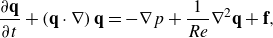 \begin{align} &\frac {\partial \textbf{q}}{\partial t} + \left (\textbf{q} \cdot \nabla \right )\textbf{q} = -\nabla p + \frac {1}{Re} \nabla ^2 \textbf{q} + \textbf{f}, \end{align}
 \begin{align} &\qquad\qquad\qquad \nabla \cdot \textbf{q}=0, \end{align}
with $\textbf{q}= ( q_1(\textbf{x},t),q_2(\textbf{x},t),q_3(\textbf{x},t) )^{\textsf{T}}$
representing the velocity vector,
$\textbf{q}= ( q_1(\textbf{x},t),q_2(\textbf{x},t),q_3(\textbf{x},t) )^{\textsf{T}}$
representing the velocity vector, $p=p(\textbf{x},t)$
the pressure field,
$p=p(\textbf{x},t)$
the pressure field, $\textbf{f}$
a body force and
$\textbf{f}$
a body force and $Re=cU_\infty /\nu =5.33\times 10^{5}$
the Reynolds number, based on the chord
$Re=cU_\infty /\nu =5.33\times 10^{5}$
the Reynolds number, based on the chord $c$
, viscosity
$c$
, viscosity $\nu$
and free-stream velocity
$\nu$
and free-stream velocity $U_\infty$
. Accordingly, length scales are made non-dimensional with the chord, and velocities with the free-stream velocity, which is the format these quantities will be presented in throughout the document. The equations are solved in the Cartesian coordinates
$U_\infty$
. Accordingly, length scales are made non-dimensional with the chord, and velocities with the free-stream velocity, which is the format these quantities will be presented in throughout the document. The equations are solved in the Cartesian coordinates $\textbf{x}=(x_1,x_2,x_3)^{\textsf{T}}$
, but some quantities in this document will be expressed in the natural coordinates
$\textbf{x}=(x_1,x_2,x_3)^{\textsf{T}}$
, but some quantities in this document will be expressed in the natural coordinates $(x_s,x_n)$
, corresponding to the wall tangent and normal directions, respectively. A schematic of the domain together with the coordinate system is presented in figure 1, which corresponds to the geometry used in Faúndez Alarcón et al. (Reference Faúndez Alarcón, Morra, Hanifi and Henningson2022b
) with a span length of
$(x_s,x_n)$
, corresponding to the wall tangent and normal directions, respectively. A schematic of the domain together with the coordinate system is presented in figure 1, which corresponds to the geometry used in Faúndez Alarcón et al. (Reference Faúndez Alarcón, Morra, Hanifi and Henningson2022b
) with a span length of $L_{x_3}=0.07$
, but considering a longer domain along the streamwise direction.
$L_{x_3}=0.07$
, but considering a longer domain along the streamwise direction.
The set (2.1) is solved using the spectral element code Nek5000 (Fischer et al. Reference Fischer, Kruse, Mullen, Tufo, Lottes and Kerkemeier2008). Here, the spatial discretisation is done considering a ![]() formulation, with the velocity field expanded on Lagrange polynomial defined on
formulation, with the velocity field expanded on Lagrange polynomial defined on $N$
Gauss–Lobatto–Legendre nodes, and the pressure field on
$N$
Gauss–Lobatto–Legendre nodes, and the pressure field on $N-2$
staggered Gauss–Legendre nodes. The solution is marched in time by a semi-implicit scheme, where the viscous terms are treated implicitly with a second-order backward differentiation while the nonlinear terms are computed explicitly through an extrapolation method of the same order. In these simulations, the number of spectral elements corresponds to
$N-2$
staggered Gauss–Legendre nodes. The solution is marched in time by a semi-implicit scheme, where the viscous terms are treated implicitly with a second-order backward differentiation while the nonlinear terms are computed explicitly through an extrapolation method of the same order. In these simulations, the number of spectral elements corresponds to $N_{x_s}\times N_{x_n} \times N_{x_3} = 230\times 30 \times 45=3\,10\,500$
, and a polynomial order equal to 7 in each element direction.
$N_{x_s}\times N_{x_n} \times N_{x_3} = 230\times 30 \times 45=3\,10\,500$
, and a polynomial order equal to 7 in each element direction.
Domain and boundary conditions considered for the numerical simulations. The rows of sensors and actuators are shown in red and blue, respectively.
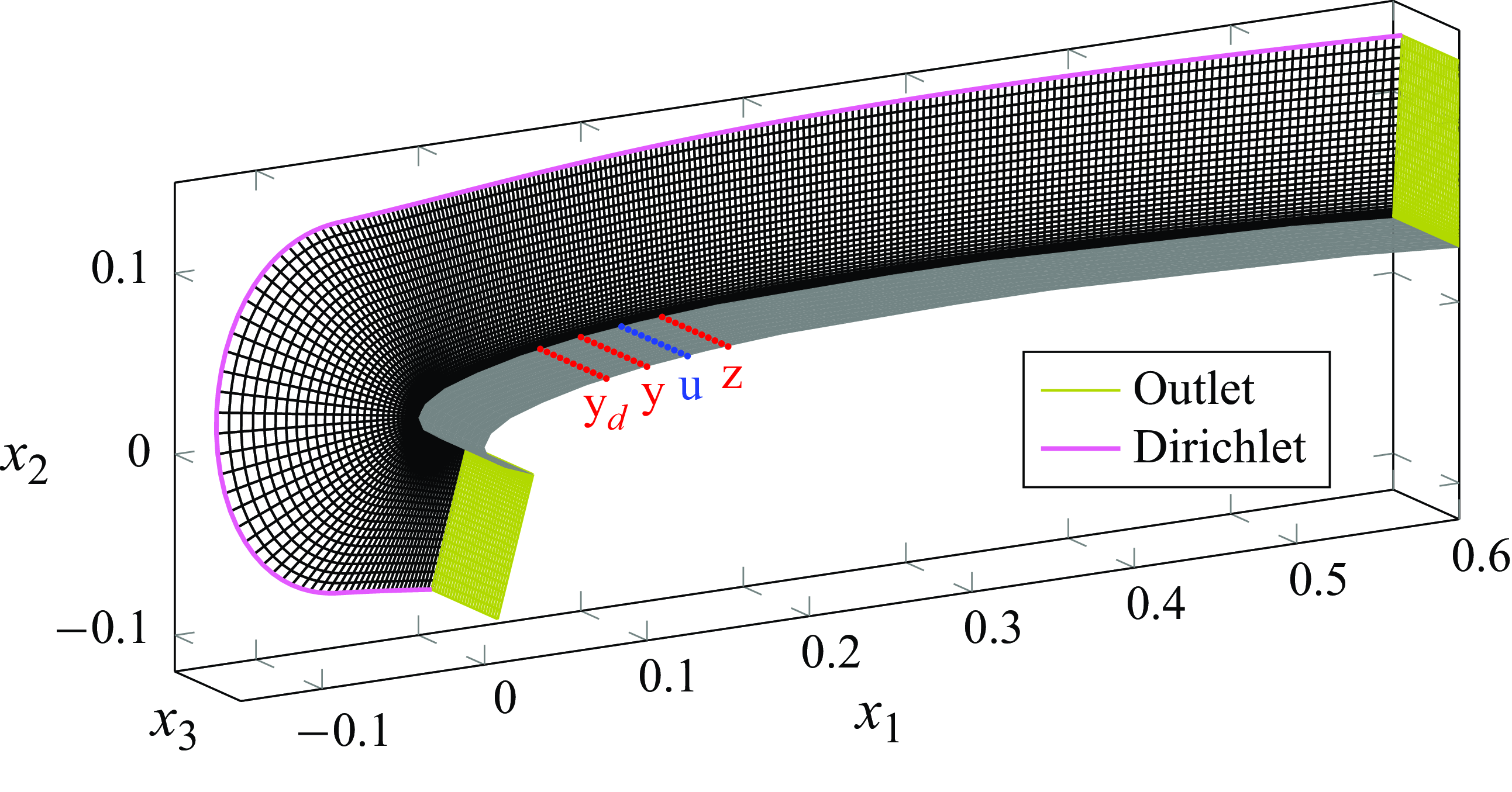
Regarding the boundary conditions, periodicity is imposed along the spanwise direction $x_3$
and no slip at the wing surface. For the outer part of the domain and the two outlets, we rely on a precursor two-dimensional simulation, where its solution,
$x_3$
and no slip at the wing surface. For the outer part of the domain and the two outlets, we rely on a precursor two-dimensional simulation, where its solution, $\textbf{q}_{BF}$
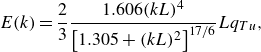
, is used to impose Dirichlet boundary conditions in the free stream, while the outlet boundary condition is defined as a stress-free condition
$\textbf{q}_{BF}$
, is used to impose Dirichlet boundary conditions in the free stream, while the outlet boundary condition is defined as a stress-free condition
 \begin{equation} \frac {1}{Re}\left (\textbf{n}\cdot \nabla \textbf{q}\right ) -p\textbf{n}=-p_a\textbf{n}, \end{equation}
where $\textbf{n}$
is the surface normal unitary vector and
$\textbf{n}$
is the surface normal unitary vector and $p_a$
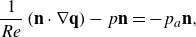
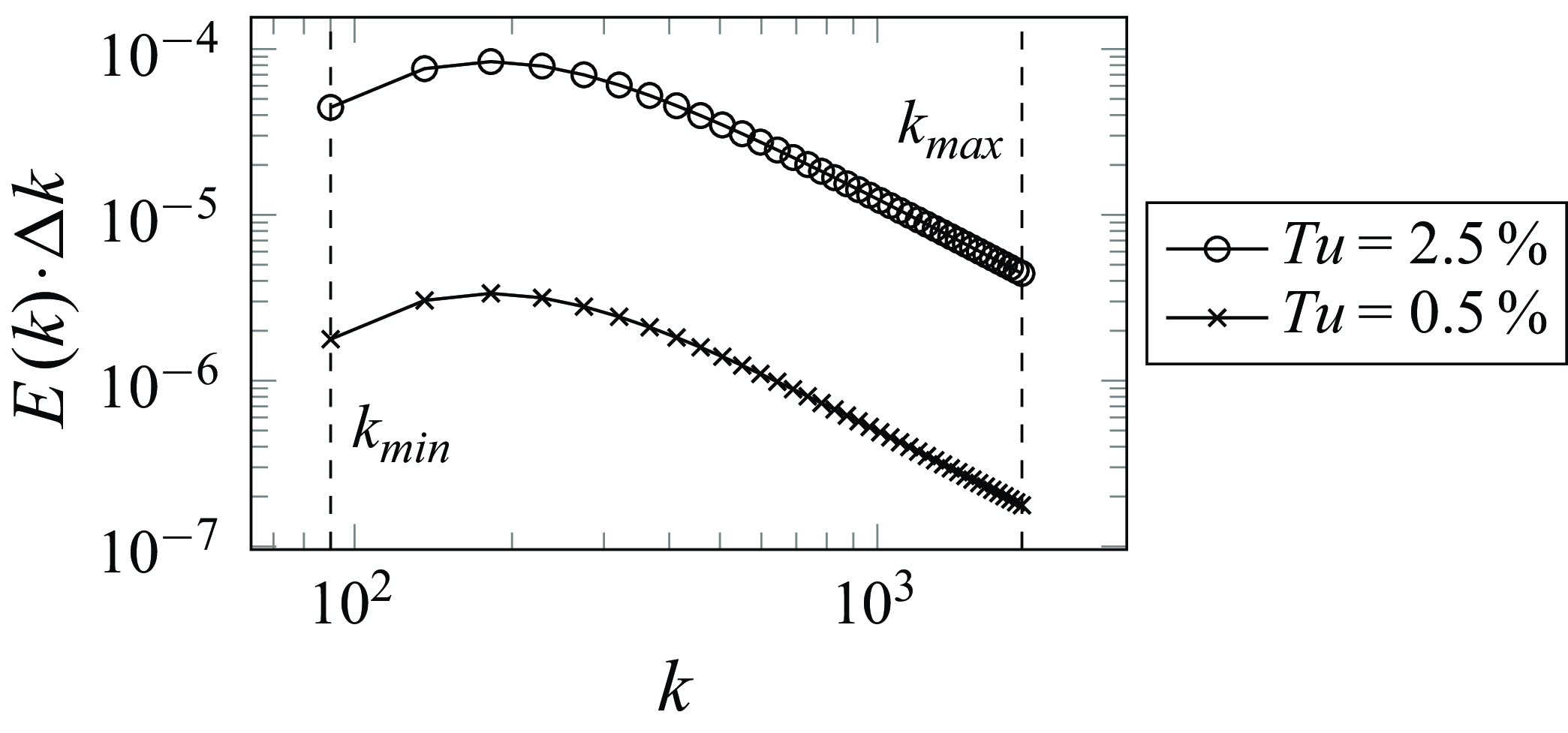
the pressure field coming from the two-dimensional simulation. Free-stream turbulence is synthesised from random Fourier modes following the Von Kármán spectrum
$p_a$
the pressure field coming from the two-dimensional simulation. Free-stream turbulence is synthesised from random Fourier modes following the Von Kármán spectrum
 \begin{equation} E(k) = \frac {2}{3} \frac {1.606(kL)^4}{\left [1.305+(kL)^2\right ]^{17/6}} Lq_{Tu}, \end{equation}
with $E$
being the energy for the total wavenumber
$E$
being the energy for the total wavenumber $k=\sqrt {k_{x_1}^2+k_{x_2}^2+k_{x_3}^2}$
,
$k=\sqrt {k_{x_1}^2+k_{x_2}^2+k_{x_3}^2}$
, $L$
the turbulence length scale and
$L$
the turbulence length scale and $q_{Tu}= 3/2Tu^2$
the total turbulence kinetic energy and
$q_{Tu}= 3/2Tu^2$
the total turbulence kinetic energy and $Tu$
is the turbulence intensity. The spectrum (2.3) is discretised with 40 equidistant wavenumbers
$Tu$
is the turbulence intensity. The spectrum (2.3) is discretised with 40 equidistant wavenumbers $k$
in the range
$k$
in the range $k_{min }=90$
to
$k_{min }=90$
to $k_{max }=1890$
, which is shown in figure 2. For each discrete total wavenumber, the energy is divided into 40 random wavenumber combinations
$k_{max }=1890$
, which is shown in figure 2. For each discrete total wavenumber, the energy is divided into 40 random wavenumber combinations $\textbf{k}=(k_{x_1},k_{x_2},k_{x_3})$
, while respecting the periodic condition along
$\textbf{k}=(k_{x_1},k_{x_2},k_{x_3})$
, while respecting the periodic condition along $x_3$
, leading to a total 1600 Fourier modes. The amplitude
$x_3$
, leading to a total 1600 Fourier modes. The amplitude $|\textbf{q}_i'|$
of the
$|\textbf{q}_i'|$
of the $i$
Fourier mode is dictated by (2.3), while its direction is randomly chosen but forced to satisfy the continuity condition
$i$
Fourier mode is dictated by (2.3), while its direction is randomly chosen but forced to satisfy the continuity condition $\textbf{q}'_i\cdot \textbf{k}_i=0$
. The random perturbations
$\textbf{q}'_i\cdot \textbf{k}_i=0$
. The random perturbations $\textbf{q}_i'$
enter the domain as Dirichlet boundary condition on top of
$\textbf{q}_i'$
enter the domain as Dirichlet boundary condition on top of $\textbf{q}_{BF}$
in front of the leading edge.
$\textbf{q}_{BF}$
in front of the leading edge.
Only one turbulence length scale $L=0.01$
and two turbulence intensities
$L=0.01$
and two turbulence intensities $Tu=\{0.5\,\%,2.5\,\%\}$
were considered in this work. Compared with the previous investigations to this work (Morra et al. Reference Morra, Sasaki, Hanifi, Cavalieri and Henningson2019; Sasaki et al. Reference Sasaki, Morra, Cavalieri, Hanifi and Henningson2019), the integral length scale was chosen to be closer to values that are more likely found in grid-generated turbulence (see, for instance, Jonáš et al. Reference Jonáš, Mazur and Uruba2000; Fransson & Shahinfar Reference Fransson and Shahinfar2020). At the same time, it is desirable to keep the value as small as possible to save computational time by limiting the spanwise extension. The choice of the integral length scale has implications for the flow dynamics, and, as will be shown, has consequences for the control design and performance. More details about the spectrum can be found in Faúndez Alarcón et al. (Reference Faúndez Alarcón, Morra, Hanifi and Henningson2022b
), while more examples on the use of this method for FST generation can be found, for instance, in Brandt et al. (Reference Brandt, Schlatter and Henningson2004), Negi (Reference Negi2019), Durović et al. (Reference Durović, De, Luca, Daniele, Davide, Jan, Dan and Hanifi2021) and De Vincentiis et al. (Reference De, Luca, Dan and Hanifi2022).
$Tu=\{0.5\,\%,2.5\,\%\}$
were considered in this work. Compared with the previous investigations to this work (Morra et al. Reference Morra, Sasaki, Hanifi, Cavalieri and Henningson2019; Sasaki et al. Reference Sasaki, Morra, Cavalieri, Hanifi and Henningson2019), the integral length scale was chosen to be closer to values that are more likely found in grid-generated turbulence (see, for instance, Jonáš et al. Reference Jonáš, Mazur and Uruba2000; Fransson & Shahinfar Reference Fransson and Shahinfar2020). At the same time, it is desirable to keep the value as small as possible to save computational time by limiting the spanwise extension. The choice of the integral length scale has implications for the flow dynamics, and, as will be shown, has consequences for the control design and performance. More details about the spectrum can be found in Faúndez Alarcón et al. (Reference Faúndez Alarcón, Morra, Hanifi and Henningson2022b
), while more examples on the use of this method for FST generation can be found, for instance, in Brandt et al. (Reference Brandt, Schlatter and Henningson2004), Negi (Reference Negi2019), Durović et al. (Reference Durović, De, Luca, Daniele, Davide, Jan, Dan and Hanifi2021) and De Vincentiis et al. (Reference De, Luca, Dan and Hanifi2022).
Discrete spectra considered in this work to synthesise the incoming FST.
Finally, and to avoid numerically destabilising backflow at the outlets, a sponge region of the form
 \begin{equation} \textbf{f}_{\lambda }(\textbf{x},t) = \lambda (\textbf{x})\left (\textbf{q}_{BF}(\textbf{x})-\textbf{q}(\textbf{x},t)\right ), \end{equation}
is imposed before the outlets. Here, $\textbf{f}_{\lambda }$
is a forcing term in (2.1) that drives the flow to the base flow
$\textbf{f}_{\lambda }$
is a forcing term in (2.1) that drives the flow to the base flow $\textbf{q}_{BF}$
before leaving the domain, and
$\textbf{q}_{BF}$
before leaving the domain, and $\lambda$
a non-negative function with support in the sponge region only. The extension of the sponge regions for both outlets was set to
$\lambda$
a non-negative function with support in the sponge region only. The extension of the sponge regions for both outlets was set to $\Delta x_1=0.025$
.
$\Delta x_1=0.025$
.
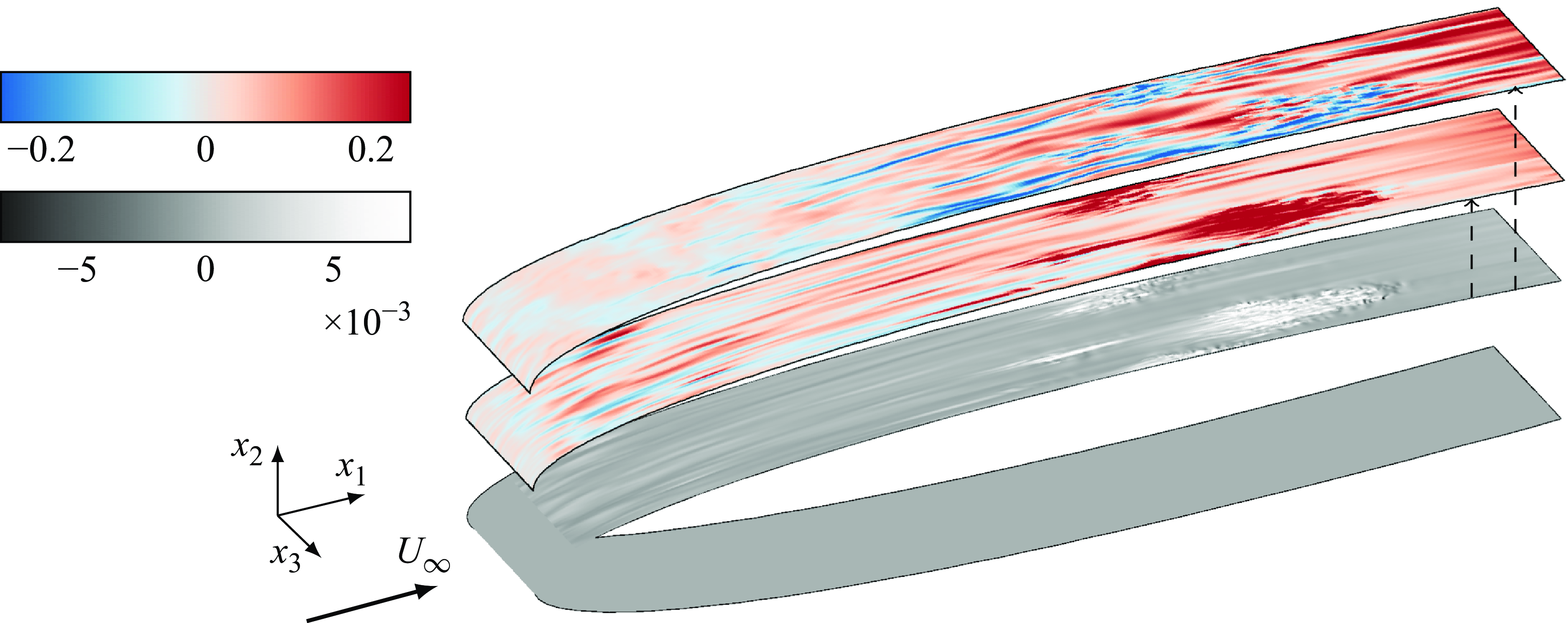
Figure 3 includes three wall-normal planes at an arbitrary snapshot of the uncontrolled simulation with $Tu=2.5\,\%$
, showing the main features of the boundary-layer response to FST. The two planes above the wing surface show streaks at different stages of their development inside the boundary layer, with a few turbulent spots producing high shear at the wall (white contours on the wing surface). This figure serves as a good representation to motivate our control goal in damping the streaks to avoid their breakdown, and as a result, avoid the large shear associated with this.
$Tu=2.5\,\%$
, showing the main features of the boundary-layer response to FST. The two planes above the wing surface show streaks at different stages of their development inside the boundary layer, with a few turbulent spots producing high shear at the wall (white contours on the wing surface). This figure serves as a good representation to motivate our control goal in damping the streaks to avoid their breakdown, and as a result, avoid the large shear associated with this.
Wall-normal planes at an arbitrary snapshot ( $Tu=2.5\,\%$
). The red and blue contours represent the positive and negative streamwise velocity perturbations, respectively, at two wall-normal planes from the wing surface. The grey contours represent the shear at the wall. Note that the lower face of the wing has been included for better visualisation, but only a small fraction of it is part of the numerical domain.
$Tu=2.5\,\%$
). The red and blue contours represent the positive and negative streamwise velocity perturbations, respectively, at two wall-normal planes from the wing surface. The grey contours represent the shear at the wall. Note that the lower face of the wing has been included for better visualisation, but only a small fraction of it is part of the numerical domain.
2.2. Controller configuration
Throughout this work, the configuration of the controller involving the placement and type of sensors and actuators is fixed, corresponding to rows of localised and equidistant devices along the span, as shown in figure 1. The only two parameters that vary are the number of sensors/actuators along the span and, accordingly, the spanwise size of the sensors/actuators. Here, $N_{y_d}$
sensors are placed at
$N_{y_d}$
sensors are placed at $x_{1,y_d}=0.075$
,
$x_{1,y_d}=0.075$
, $N_y$
sensors at
$N_y$
sensors at $x_{1,y}=0.1$
,
$x_{1,y}=0.1$
, $N_u$
actuators at
$N_u$
actuators at $x_{1,u}=0.125$
and
$x_{1,u}=0.125$
and $N_z$
sensors at
$N_z$
sensors at $x_{1,z}=0.15$
. The precise role of these devices will be explained in the next section, but it is worth noting now that, for a given case, the condition
$x_{1,z}=0.15$
. The precise role of these devices will be explained in the next section, but it is worth noting now that, for a given case, the condition $N_{y_d}=N_u=N_y=N_z$
is imposed. The motivation for this choice lies on the three-dimensional nature of the disturbance to be controlled, the homogenous base flow and the random appearance of turbulent spots along the span.
$N_{y_d}=N_u=N_y=N_z$
is imposed. The motivation for this choice lies on the three-dimensional nature of the disturbance to be controlled, the homogenous base flow and the random appearance of turbulent spots along the span.
The position of the control devices was based on physical and performance considerations. In this respect, there exists a trade-off between placing the devices close or farther away from the leading edge. Closer to the leading edge, the disturbances have a lower amplitude, and therefore it would require less control effort to damp them. However, in this early stage of receptivity, the boundary layer has not yet filtered out disturbances that will decay downstream and they are consequently less relevant for the transition process. It would be tempting then to place the devices far downstream, where only the most amplified disturbances are present. This has the drawback that nonlinear interactions become more prominent downstream, which could affect the performance of a linear controller. Besides, the scattered appearance in time and space of turbulent spots forces us to be conservative regarding how far downstream the devices can be placed.
The relative position between rows of sensors and actuators represents a feedforward configuration, where the actuation ( $\textbf{u}$
) is based on measurements upstream (
$\textbf{u}$
) is based on measurements upstream ( $\textbf{y}$
) to minimise another set of measurements downstream (
$\textbf{y}$
) to minimise another set of measurements downstream ( $\textbf{z}$
). This type of arrangement is more effective in controlling amplifier flows (Belson et al. Reference Belson, Semeraro, Rowley and Henningson2013; Sipp & Schmid Reference Sipp and Schmid2016), as is the case of a boundary layer. Moreover, an extra benefit of this configuration is that robustness regarding stability of the controller is guaranteed (Sipp & Schmid Reference Sipp and Schmid2016).
$\textbf{z}$
). This type of arrangement is more effective in controlling amplifier flows (Belson et al. Reference Belson, Semeraro, Rowley and Henningson2013; Sipp & Schmid Reference Sipp and Schmid2016), as is the case of a boundary layer. Moreover, an extra benefit of this configuration is that robustness regarding stability of the controller is guaranteed (Sipp & Schmid Reference Sipp and Schmid2016).
Similarly to the work by Morra et al. (Reference Morra, Sasaki, Hanifi, Cavalieri and Henningson2019) and Sasaki et al. (Reference Sasaki, Morra, Cavalieri, Hanifi and Henningson2019), the sensors are localised at the wall and measure the perturbation streamwise wall shear as
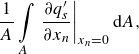 \begin{equation} \frac {1}{A}\int \limits _A \left .\frac {\partial q_s'}{\partial x_n}\right |_{x_n=0} \textrm{d}A, \end{equation}
where $A$
corresponds to the area of the sensor given by the radius
$A$
corresponds to the area of the sensor given by the radius $r=L_{x_3}/(2N_y)$
and
$r=L_{x_3}/(2N_y)$
and $q_s'$
is the streamwise velocity perturbation. The sensor size was chosen to avoid overlap between consecutive devices. These time-dependent signals will be referred to as the outputs of the system, and correspond to the quantities
$q_s'$
is the streamwise velocity perturbation. The sensor size was chosen to avoid overlap between consecutive devices. These time-dependent signals will be referred to as the outputs of the system, and correspond to the quantities $\textbf{d}$
,
$\textbf{d}$
, $\textbf{y}$
and
$\textbf{y}$
and $\textbf{z}$
. On the other hand, the actuators correspond to body forces in (2.1) of the form
$\textbf{z}$
. On the other hand, the actuators correspond to body forces in (2.1) of the form
 \begin{equation} \textbf{f}_{u_k}(\textbf{x},t) = u_k(t)\textbf{b}_k(\textbf{x}), \end{equation}
where $\textbf{b}_k$
is a prescribed spatial support of the force and
$\textbf{b}_k$
is a prescribed spatial support of the force and $u_k$
the time modulation signal, both quantities corresponding to the
$u_k$
the time modulation signal, both quantities corresponding to the $k$
actuator along the span. In what follows, the quantity
$k$
actuator along the span. In what follows, the quantity $\textbf{u}$
will be referred to as the input of the system, which will be computed from optimal control theory based on the available output
$\textbf{u}$
will be referred to as the input of the system, which will be computed from optimal control theory based on the available output $\textbf{y}$
to minimise the output
$\textbf{y}$
to minimise the output $\textbf{z}$
. The spatial support is defined to act only in the wall-normal direction, and takes the form
$\textbf{z}$
. The spatial support is defined to act only in the wall-normal direction, and takes the form
 \begin{align} &\qquad\qquad\qquad\quad \textbf{b}_k = \left ( 0, b_{x_n}(k), 0 \right )^{\textsf{T}}, \end{align}
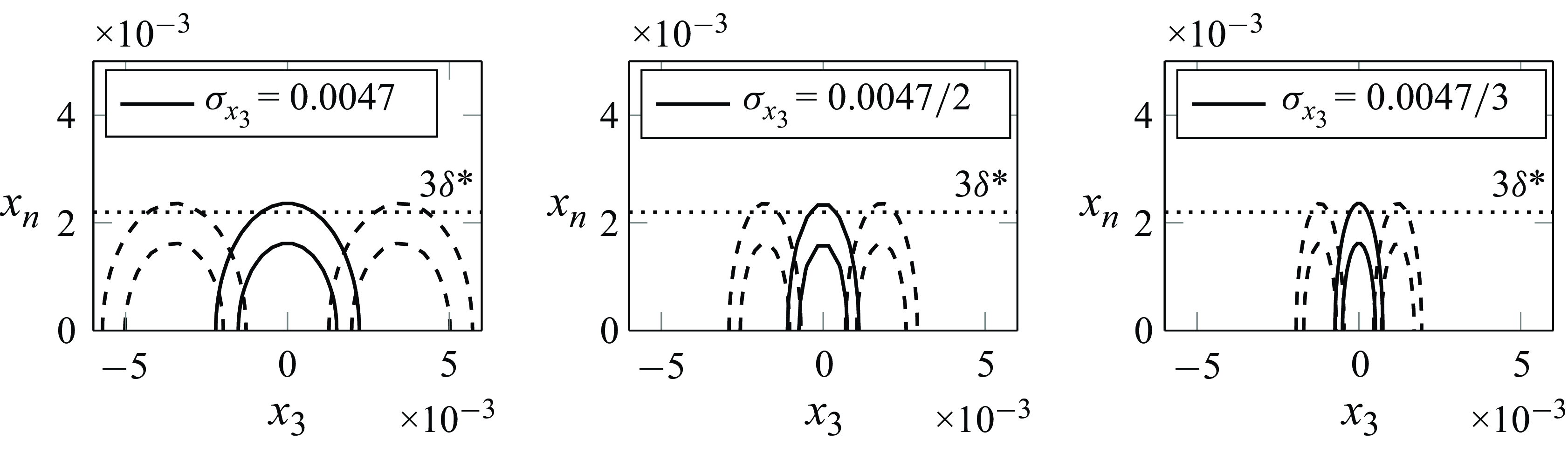
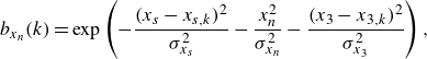 \begin{align} & b_{x_n}(k) = \exp \left ( -\frac {(x_s-x_{s,k})^2}{\sigma _{x_s}^2} -\frac {x_n^2}{\sigma _{x_n}^2}-\frac {(x_3-x_{3,k})^2}{\sigma _{x_3}^2}\right ), \end{align}
with $\textbf{x}_k = (x_{s,k},0,x_{3,k})^{\textsf{T}}$
the centre of the
$\textbf{x}_k = (x_{s,k},0,x_{3,k})^{\textsf{T}}$
the centre of the $k$
actuator at the wall and
$k$
actuator at the wall and $\sigma _{x_s}=\sigma _{x_n}=0.005$
for all the cases. These values were chosen such the actuators do not overlap with the sensors upstream and downstream, and to have significant support inside the boundary layer, since it has been shown by Sasaki et al. (Reference Sasaki, Morra, Cavalieri, Hanifi and Henningson2019) that optimal actuator shapes possess this characteristic (cf. figure 9). For the scalar
$\sigma _{x_s}=\sigma _{x_n}=0.005$
for all the cases. These values were chosen such the actuators do not overlap with the sensors upstream and downstream, and to have significant support inside the boundary layer, since it has been shown by Sasaki et al. (Reference Sasaki, Morra, Cavalieri, Hanifi and Henningson2019) that optimal actuator shapes possess this characteristic (cf. figure 9). For the scalar $\sigma _{x_3}$
, three values were considered based on the number of actuators. The shapes of the three actuators are presented in figure 4 together with their corresponding
$\sigma _{x_3}$
, three values were considered based on the number of actuators. The shapes of the three actuators are presented in figure 4 together with their corresponding $\sigma _{x_3}$
value. It can be seen that the actuators have significant support up to
$\sigma _{x_3}$
value. It can be seen that the actuators have significant support up to $3\delta ^*$
, with
$3\delta ^*$
, with $\delta ^*$
the displacement thickness at the actuator’s position. Also note that, for the first actuator,
$\delta ^*$
the displacement thickness at the actuator’s position. Also note that, for the first actuator, $\sigma _{x_3}$
is slightly smaller than
$\sigma _{x_3}$
is slightly smaller than $\sigma _{x_s}$
and
$\sigma _{x_s}$
and $\sigma _{x_n}$
, this was arbitrarily chosen but under the consideration that actuators do not overlap at the level
$\sigma _{x_n}$
, this was arbitrarily chosen but under the consideration that actuators do not overlap at the level $0.9$
, in concordance with the shapes used in Morra et al. (Reference Morra, Sasaki, Hanifi, Cavalieri and Henningson2019).
$0.9$
, in concordance with the shapes used in Morra et al. (Reference Morra, Sasaki, Hanifi, Cavalieri and Henningson2019).
Actuator shapes considered in this work. The figures show three consecutive actuators and their overlap for the contour levels $\{0.8,0.9\}$
. The
$\{0.8,0.9\}$
. The $x$
-axis only shows a portion of the span length.
$x$
-axis only shows a portion of the span length.
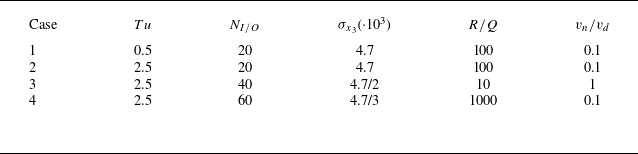
A summary of the cases under study with their relevant parameters is presented in table 1. The ratios in the last two columns correspond to parameters used in the control problem, and their significance will be elaborated on in the next section. The purpose of the simulation with $Tu=0.5\,\%$
is to evaluate the performance of the controller in a case where the dynamics of the disturbances is mostly linear, as was shown in Faúndez Alarcón et al. (Reference Faúndez Alarcón, Morra, Hanifi and Henningson2022b
). The choice of
$Tu=0.5\,\%$
is to evaluate the performance of the controller in a case where the dynamics of the disturbances is mostly linear, as was shown in Faúndez Alarcón et al. (Reference Faúndez Alarcón, Morra, Hanifi and Henningson2022b
). The choice of $N_{I/O}=20$
for this case emanates from the observation that most of the disturbance energy is contained in low spanwise wavenumbers, and solving up to the 9th wavenumber gives an accurate representation of the spectrum. On the other hand, the purpose of the cases with
$N_{I/O}=20$
for this case emanates from the observation that most of the disturbance energy is contained in low spanwise wavenumbers, and solving up to the 9th wavenumber gives an accurate representation of the spectrum. On the other hand, the purpose of the cases with $Tu=2.5\,\%$
is twofold. First, evaluating the performance of the linear controller when the nonlinear dynamics becomes more significant. And secondly, the effect it has downstream in delaying transition.
$Tu=2.5\,\%$
is twofold. First, evaluating the performance of the linear controller when the nonlinear dynamics becomes more significant. And secondly, the effect it has downstream in delaying transition.
List of cases and their corresponding parameters. $N_{I/O}$
corresponds to the number of sensors/actuators along each row.
$N_{I/O}$
corresponds to the number of sensors/actuators along each row.
3. Control law design
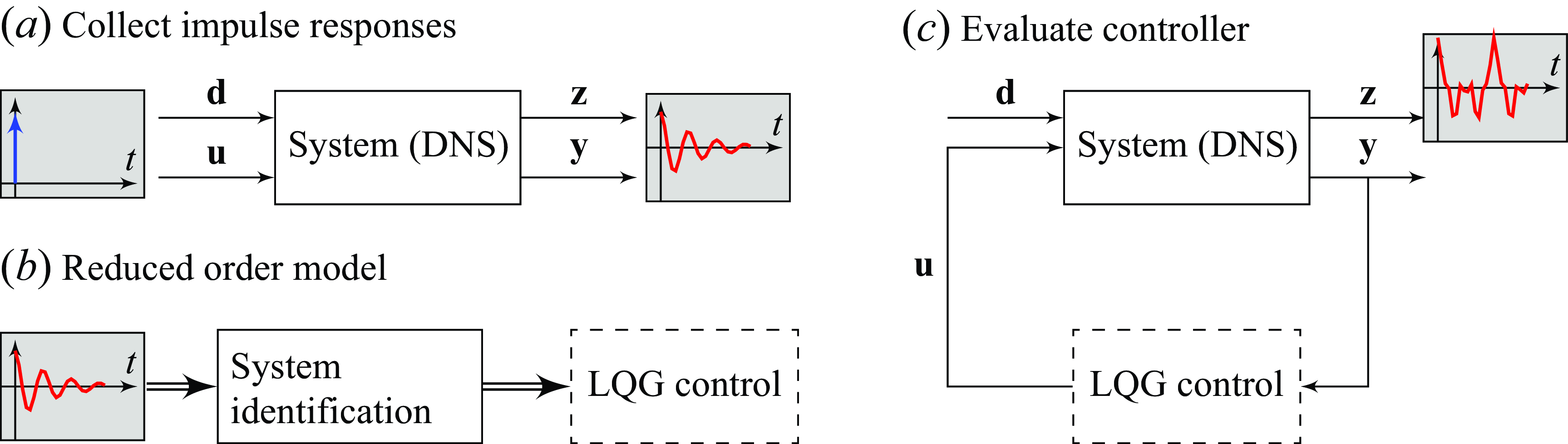
In this section, we describe the process from which we construct the control law. In this regard, we follow the procedure developed in Morra et al. (Reference Morra, Sasaki, Hanifi, Cavalieri and Henningson2019) and Sasaki et al. (Reference Sasaki, Morra, Cavalieri, Hanifi and Henningson2019) for a flat plate, wherein more details about the implementation can be found. The block diagram of the open and closed loop representation of the system is included in figure 5, and it is also added the intermediate step where the control law is designed. These represent the basic steps involved in our implementation.
Summary of the controller design, (a) starting from the collection of impulse responses of the open loop system, (b) the offline design of the model and controller and (c) the final implementation in the DNS closed loop system.
3.1. Linear–quadratic–Gaussian control
In order to design the control strategy, we rely on the dynamical system representation of the flow. By considering an equilibrium state $\textbf{q}_0$
, the state vector
$\textbf{q}_0$
, the state vector $\textbf{q}'$
describes the fluid motion of the perturbations about that equilibrium, where the state vector is decomposed as
$\textbf{q}'$
describes the fluid motion of the perturbations about that equilibrium, where the state vector is decomposed as $\textbf{q}=\textbf{q}_0+\textbf{q}' \in \mathbb{R}^{N\times 1}$
. In this scenario, a linearised system can be obtained for sufficiently small perturbation amplitude. The action of the controller on the system is governed by an input signal fed by sensor measurements, the latter corresponding to output signals. The system is also perturbed by noise environment, where the role of the actuator is to minimise the norm of a second set of measurements. With these considerations, the dynamical system can be expressed as
$\textbf{q}=\textbf{q}_0+\textbf{q}' \in \mathbb{R}^{N\times 1}$
. In this scenario, a linearised system can be obtained for sufficiently small perturbation amplitude. The action of the controller on the system is governed by an input signal fed by sensor measurements, the latter corresponding to output signals. The system is also perturbed by noise environment, where the role of the actuator is to minimise the norm of a second set of measurements. With these considerations, the dynamical system can be expressed as
 \begin{align} \dot {\textbf{q}}'(t) &= \textbf{A} \textbf{q}'(t) + \textbf{B}_u\textbf{u}(t) + \textbf{B}_d \textbf{d}(t), \end{align}
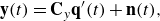 \begin{align} \textbf{y}(t) &= \textbf{C}_y \textbf{q}'(t) + \textbf{n}(t), \end{align}
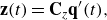 \begin{align} \textbf{z}(t) &= \textbf{C}_z \textbf{q}'(t), \end{align}
where $\textbf{A} \in \mathbb{R}^{N\times N}$
dictates the dynamics of the perturbations,
$\textbf{A} \in \mathbb{R}^{N\times N}$
dictates the dynamics of the perturbations, $\textbf{B}_u\in \mathbb{R}^{N\times N_u}$
how the input signal
$\textbf{B}_u\in \mathbb{R}^{N\times N_u}$
how the input signal $\textbf{u}(t) \in {\mathbb{R}}^{N_u\times 1}$
of the controller acts on the flow and
$\textbf{u}(t) \in {\mathbb{R}}^{N_u\times 1}$
of the controller acts on the flow and $\textbf{B}_d\in {\mathbb{R}}^{N\times N_d}$
how the stochastic noise
$\textbf{B}_d\in {\mathbb{R}}^{N\times N_d}$
how the stochastic noise $\textbf{d}(t)\in {\mathbb{R}}^{N_d\times 1}$
affects the perturbations. The matrices
$\textbf{d}(t)\in {\mathbb{R}}^{N_d\times 1}$
affects the perturbations. The matrices $\textbf{C}_y\in {\mathbb{R}}^{N_y\times N}$
and
$\textbf{C}_y\in {\mathbb{R}}^{N_y\times N}$
and $\textbf{C}_z\in {\mathbb{R}}^{N_z\times N}$
contain the information regarding of how the information is extracted from the system to obtain the outputs
$\textbf{C}_z\in {\mathbb{R}}^{N_z\times N}$
contain the information regarding of how the information is extracted from the system to obtain the outputs $\textbf{y}(t)\in {\mathbb{R}}^{N_y\times 1}$
and
$\textbf{y}(t)\in {\mathbb{R}}^{N_y\times 1}$
and $\textbf{z}(t)\in {\mathbb{R}}^{N_z\times 1}$
, respectively. The stochastic noise
$\textbf{z}(t)\in {\mathbb{R}}^{N_z\times 1}$
, respectively. The stochastic noise $\textbf{n}(t)\in {\mathbb{R}}^{N_y\times 1}$
is added to account for the contamination of the sensor signal.
$\textbf{n}(t)\in {\mathbb{R}}^{N_y\times 1}$
is added to account for the contamination of the sensor signal.
The control problem consists on finding the signal $\textbf{u}(t)$
based on the measurements
$\textbf{u}(t)$
based on the measurements $\textbf{y}(t)$
, to minimise a cost objective function
$\textbf{y}(t)$
, to minimise a cost objective function $\mathcal{J}$
, by taking into account the measurements
$\mathcal{J}$
, by taking into account the measurements $\textbf{z}(t)$
together with the input signal
$\textbf{z}(t)$
together with the input signal $\textbf{u}(t)$
, which is included to penalise excessive control energy. Hence, the cost objective function takes the form
$\textbf{u}(t)$
, which is included to penalise excessive control energy. Hence, the cost objective function takes the form
 \begin{equation} \mathcal{J}=\mathbb{E}\left [ \lim \limits _{T\to \infty }\frac {1}{T} \int \limits _0^T \textbf{z}(t)^\textsf{T}\textbf{Q}\textbf{z}(t) + \textbf{u}(t)^\textsf{T}\textbf{R}\textbf{u}(t)\textrm{d}t \right ], \end{equation}
where the matrices $\textbf{Q}$
and
$\textbf{Q}$
and $\textbf{R}$
are user-defined weights that balance the two terms in the cost function. When using a LQG controller, the optimisation problem can be separated into two independent optimisation problems: the optimal observer and the optimal feedback control problem.
$\textbf{R}$
are user-defined weights that balance the two terms in the cost function. When using a LQG controller, the optimisation problem can be separated into two independent optimisation problems: the optimal observer and the optimal feedback control problem.
The optimal feedback control problem assumes full knowledge of the system state $\textbf{q}'$
, and its solution is known as the linear –quadratic regulator (LQR). The optimisation of the cost function in (3.2) yields to a Riccati equation from which the optimal control gain
$\textbf{q}'$
, and its solution is known as the linear –quadratic regulator (LQR). The optimisation of the cost function in (3.2) yields to a Riccati equation from which the optimal control gain $\textbf{K}$
can be obtained, which is used to define the actuation signal as
$\textbf{K}$
can be obtained, which is used to define the actuation signal as $\textbf{u}=\textbf{K}\textbf{q}'$
. Here, the matrix
$\textbf{u}=\textbf{K}\textbf{q}'$
. Here, the matrix $\textbf{P}$
is the unknown of the Riccati equation
$\textbf{P}$
is the unknown of the Riccati equation
 \begin{equation} \textbf{A}^{\textsf{T}}\textbf{P} + \textbf{P}\textbf{A} - \textbf{P}\textbf{B}_u\textbf{R}^{-1}\textbf{B}_u^{\textsf{T}}\textbf{P} + \textbf{C}_z^{\textsf{T}} \textbf{Q} \textbf{C}_z=0, \end{equation}
from which the optimal control gain is obtained as
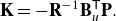 \begin{equation} \textbf{K} = -\textbf{R}^{-1}\textbf{B}_u^{\textsf{T}} \textbf{P}. \end{equation}
As mentioned before, this optimal gain assumes full access to the state vector $\textbf{q}'$
, which is not always feasible to obtain and in most cases one is limited to the output
$\textbf{q}'$
, which is not always feasible to obtain and in most cases one is limited to the output $\textbf{y}$
to decide the control action. This results in the estimator problem, where the goal is to obtain an approximation
$\textbf{y}$
to decide the control action. This results in the estimator problem, where the goal is to obtain an approximation $\tilde {\textbf{q}}'$
of the vector state
$\tilde {\textbf{q}}'$
of the vector state $\textbf{q}'$
based exclusively on the measurements
$\textbf{q}'$
based exclusively on the measurements $\textbf{y}$
. The estimation state
$\textbf{y}$
. The estimation state $\tilde {\textbf{q}}'$
is described by an identical system as (3.1), where the noise is ignored, and the estimator is forced by
$\tilde {\textbf{q}}'$
is described by an identical system as (3.1), where the noise is ignored, and the estimator is forced by $-\textbf{L}(\textbf{y}-\tilde {\textbf{y}})$
, penalising the differences between the true measurements
$-\textbf{L}(\textbf{y}-\tilde {\textbf{y}})$
, penalising the differences between the true measurements $\textbf{y}$
and its estimation
$\textbf{y}$
and its estimation $\tilde {\textbf{y}}$
. This new system therefore reads
$\tilde {\textbf{y}}$
. This new system therefore reads
 \begin{align} \dot {\tilde {\textbf{q}}}'(t) &= \textbf{A} \tilde {\textbf{q}}'(t) + \textbf{B}_u\textbf{u}(t) - \textbf{L}(\textbf{y}(t)-\tilde {\textbf{y}}(t)), \end{align}
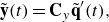 \begin{align} \tilde {\textbf{y}}(t) &= \textbf{C}_y \tilde {\textbf{q}}'(t), \end{align}
 \begin{align} \textbf{e}(t) &= \textbf{q}'(t) - \tilde {\textbf{q}}'(t). \end{align}
By minimising the norm of the error $\textbf{e}(t)$
while satisfying the governing equations, we end up with the linear–quadratic estimation (LQE) problem, whose solution is given by the Riccati equation
$\textbf{e}(t)$
while satisfying the governing equations, we end up with the linear–quadratic estimation (LQE) problem, whose solution is given by the Riccati equation
 \begin{equation} \textbf{S}\textbf{A}^{\textsf{T}} + \textbf{A}\textbf{S} - \textbf{S}\textbf{C}_y^{\textsf{T}}\textbf{V}_n^{-1}\textbf{C}_y^{\textbf{S}} + \textbf{B}_d \textbf{V}_d \textbf{B}_d^{\textsf{T}}=0, \end{equation}
where $\textbf{S}$
is the unknown, and
$\textbf{S}$
is the unknown, and $\textbf{V}_n$
and
$\textbf{V}_n$
and $\textbf{V}_d$
are the covariances of the sensor and background noise, respectively. The optimal
$\textbf{V}_d$
are the covariances of the sensor and background noise, respectively. The optimal $\textbf{L}$
is referred to as the Kalman gain and can be computed as
$\textbf{L}$
is referred to as the Kalman gain and can be computed as
 \begin{equation} \textbf{L} = -\textbf{S}\textbf{C}_y^{\textsf{T}}\textbf{V}_n^{-1}. \end{equation}
The separation principle, that allows us to solve independently the LQR and LQE problems, has also the implication that the estimator $\tilde {\textbf{q}}'$
can be used instead of
$\tilde {\textbf{q}}'$
can be used instead of $\textbf{q}'$
to obtain the input signal
$\textbf{q}'$
to obtain the input signal $\textbf{u}$
through the optimal gain
$\textbf{u}$
through the optimal gain $\textbf{K}$
. Therefore, with the available output
$\textbf{K}$
. Therefore, with the available output $\textbf{y}(t)$
and by ignoring the initial state
$\textbf{y}(t)$
and by ignoring the initial state $\tilde {\textbf{q}}' (0)$
, the input signal can be computed from
$\tilde {\textbf{q}}' (0)$
, the input signal can be computed from
 \begin{align} &\textbf{u}(t) = - \int \limits _0^t \textbf{K}e^{\left (\textbf{A}+\textbf{B}_u \textbf{K}+\textbf{L}\textbf{C}_y\right )(t-\tau )}\textbf{L}\textbf{y}(\tau ) \textrm{d}\tau, \end{align}
 \begin{align} &\qquad\qquad= - \int \limits _0^t \mathcal{K}(t-\tau )\textbf{y}(\tau ) \textrm{d}\tau, \end{align}
where $\mathcal{K} \in \mathbb{R}^{N_u\times N_y}$
will be referred to as the control kernel. Alternatively, the control signal in (3.8) can be obtained by solving the first-order differential equations of the controller in state-space form as in Nibourel et al. (Reference Nibourel, Leclercq, Demourant, Garnier and Sipp2023). This second approach could benefit in terms of calculation costs from further reductions in the order
$\mathcal{K} \in \mathbb{R}^{N_u\times N_y}$
will be referred to as the control kernel. Alternatively, the control signal in (3.8) can be obtained by solving the first-order differential equations of the controller in state-space form as in Nibourel et al. (Reference Nibourel, Leclercq, Demourant, Garnier and Sipp2023). This second approach could benefit in terms of calculation costs from further reductions in the order $N$
of the model. Such a reduction could be achieved, for example, by choosing a larger threshold in the eigensystem realisation algorithm (ERA) described below, or by removing unnecessary delays originated from the convective character of the flow (Nibourel et al. Reference Nibourel, Leclercq, Demourant, Garnier and Sipp2023).
$N$
of the model. Such a reduction could be achieved, for example, by choosing a larger threshold in the eigensystem realisation algorithm (ERA) described below, or by removing unnecessary delays originated from the convective character of the flow (Nibourel et al. Reference Nibourel, Leclercq, Demourant, Garnier and Sipp2023).
3.2. Reduced-order model
One of the main limitations in the application of LQG is the size of the state vector, which in this case would be three times the number of grid points, and therefore of the order of a hundred million points. For this reason, a reduced-order model (ROM) is first built based only on input–output data coming from the DNS.
To construct the ROM, the ERA (Juang & Pappa Reference Juang and Pappa1985) is employed. Two main benefits of the algorithm are that it is based on input–output data of the system, and it leads to a state-space representation of the system as in (3.1), where the LQG can be designed directly. Moreover, Ma et al. (Reference Ma, Ahuja and Rowley2011) showed that, for linear systems, ERA produces the same ROM as the one obtained from balanced proper orthogonal decomposition, without the need of an adjoint system and at lower computational cost.
The algorithm relies on the impulse response from the inputs, $\textbf{u}$
and
$\textbf{u}$
and $\textbf{d}$
, to the outputs,
$\textbf{d}$
, to the outputs, $\textbf{y}$
and
$\textbf{y}$
and $\textbf{z}$
. Assuming that the impulse responses were collected for
$\textbf{z}$
. Assuming that the impulse responses were collected for $2N_t+2$
steps, we build the Hankel matrices
$2N_t+2$
steps, we build the Hankel matrices $H_0, H_1\in \mathbb{R}^{N_O(N_t+1)\times N_I(N_t+1)}$
, where
$H_0, H_1\in \mathbb{R}^{N_O(N_t+1)\times N_I(N_t+1)}$
, where $N_O=N_y+N_z$
and
$N_O=N_y+N_z$
and $N_I=N_u+N_d$
are the total number of outputs and inputs, respectively. Here,
$N_I=N_u+N_d$
are the total number of outputs and inputs, respectively. Here, $H_0$
is built with the time steps
$H_0$
is built with the time steps $i_t=1,\ldots, 2N_t+1$
, while
$i_t=1,\ldots, 2N_t+1$
, while $H_1$
with
$H_1$
with $i_t=2,\ldots, 2N_t+2$
. From the singular value decomposition (SVD) of
$i_t=2,\ldots, 2N_t+2$
. From the singular value decomposition (SVD) of $H_0$
together with the Hankel matrix
$H_0$
together with the Hankel matrix $H_1$
, the ERA constructs the reduced version of the dynamical system in (3.1), giving the system
$H_1$
, the ERA constructs the reduced version of the dynamical system in (3.1), giving the system $(\textbf{A}_r,\textbf{B}_{u,r},\textbf{B}_{d,r},\textbf{C}_{y,r},\textbf{C}_{z,r})$
which is used to design the LQG. The subscript
$(\textbf{A}_r,\textbf{B}_{u,r},\textbf{B}_{d,r},\textbf{C}_{y,r},\textbf{C}_{z,r})$
which is used to design the LQG. The subscript $r$
denotes the reduced version of the system, but also represents the
$r$
denotes the reduced version of the system, but also represents the $r$
singular value from which the SVD is truncated. In this case, this value is chosen based on the condition
$r$
singular value from which the SVD is truncated. In this case, this value is chosen based on the condition $\sigma _r/\sigma _1\gt 10^{-3}$
, with
$\sigma _r/\sigma _1\gt 10^{-3}$
, with $\sigma _1$
being the largest singular value. More details about the ERA and how we build the Hankel matrices are included in Appendix A.
$\sigma _1$
being the largest singular value. More details about the ERA and how we build the Hankel matrices are included in Appendix A.
The impulse responses are obtained directly from the DNS. The first set of impulse responses, from the actuation input $\textbf{u}$
to the outputs
$\textbf{u}$
to the outputs $\textbf{y}$
and
$\textbf{y}$
and $\textbf{z}$
, is more straightforward to obtain, and where some simplifications are possible. Due to the convective nature of the flow and the feedforward configuration of the controller, by placing the output
$\textbf{z}$
, is more straightforward to obtain, and where some simplifications are possible. Due to the convective nature of the flow and the feedforward configuration of the controller, by placing the output $\textbf{y}$
upstream of the input
$\textbf{y}$
upstream of the input $\textbf{u}$
, the response
$\textbf{u}$
, the response $\textbf{u}\to \textbf{y}$
is equal to zero. Moreover, given that the base flow is homogeneous in the spanwise direction, the periodicity along the same coordinate in the simulations, and the fact that the rows of actuators and sensors are composed by identical units, only one simulation of the impulse response from one actuator is needed. Those time signals are then repeated and translated along the spanwise direction to get the full set
$\textbf{u}\to \textbf{y}$
is equal to zero. Moreover, given that the base flow is homogeneous in the spanwise direction, the periodicity along the same coordinate in the simulations, and the fact that the rows of actuators and sensors are composed by identical units, only one simulation of the impulse response from one actuator is needed. Those time signals are then repeated and translated along the spanwise direction to get the full set $\textbf{u}\to \textbf{z}$
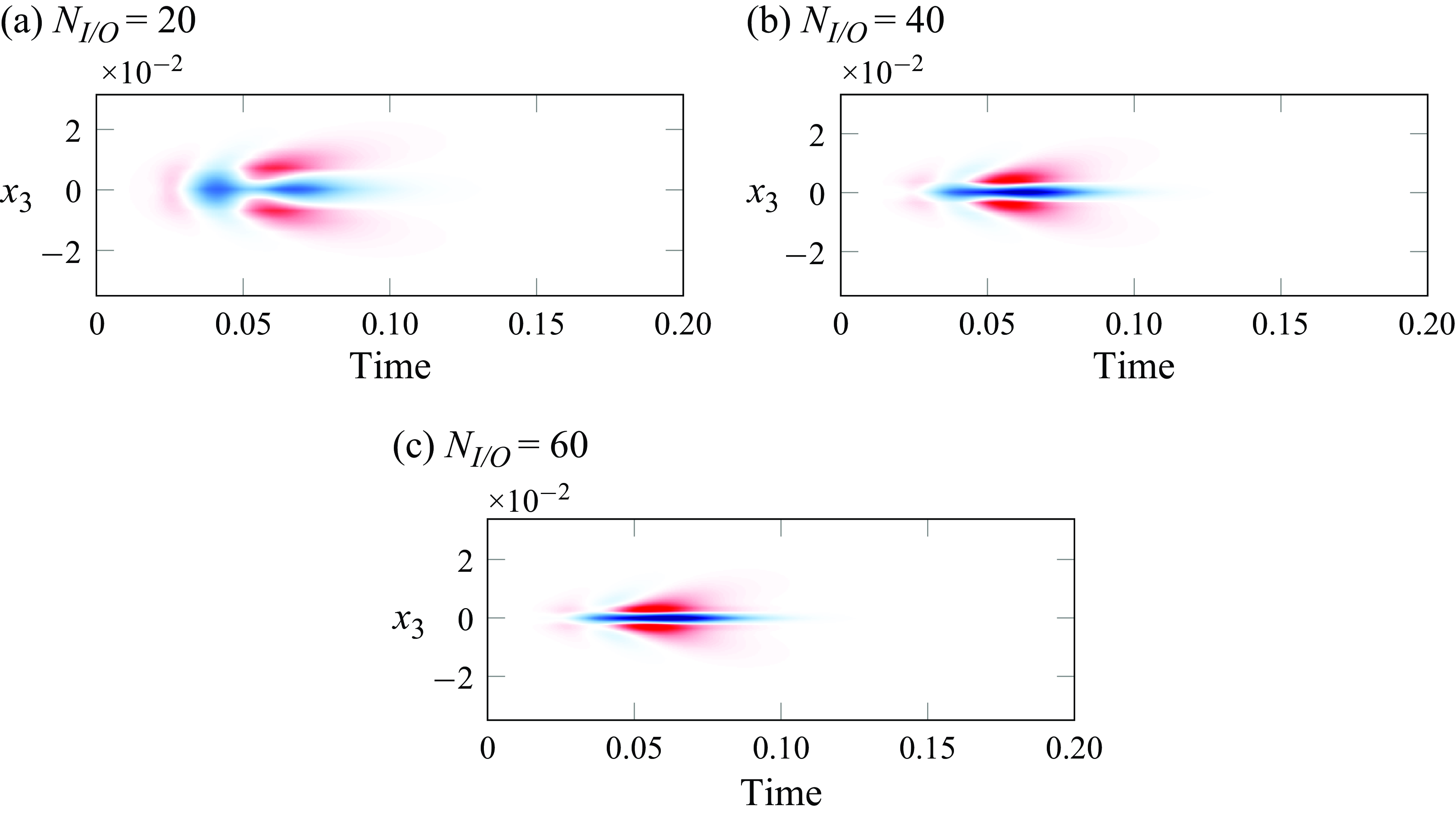
. The impulse responses for the three actuators considered in this work are presented in figure 6, showing the sensors measurements
$\textbf{u}\to \textbf{z}$
. The impulse responses for the three actuators considered in this work are presented in figure 6, showing the sensors measurements $\textbf{z}$
. These will be referred to as
$\textbf{z}$
. These will be referred to as $g_{uz}(t,k)$
, with
$g_{uz}(t,k)$
, with $k$
representing the index of the sensor.
$k$
representing the index of the sensor.
Impulse responses from one actuator centred at $x_3=0$
to the objective position. The contours represent the sensors measurements with the same colour bar for all figures.
$x_3=0$
to the objective position. The contours represent the sensors measurements with the same colour bar for all figures.
Computing the impulse responses from the disturbances to outputs, $\textbf{d}\to \textbf{y}$
and
$\textbf{d}\to \textbf{y}$
and $\textbf{d}\to \textbf{z}$
, is more challenging in this type of flow configuration. The reason behind this is the broadband spectrum in the free stream that is forcing the boundary layer, which in this case was synthesised with 1600 Fourier modes. Therefore, this would not only require the same number of simulations to be performed, but also the SVD of a much larger Hankel matrix. Arguably, only a fraction of these modes can be amplified, and hence be made relevant, by the boundary layer. This would require a receptivity analysis to discriminate the modes of interest, but with no guarantee that the reduction in number of modes will be significant. Moreover, such an impulse response study is not feasible in experiments, and even with simulations one could miss modes that can be nonlinearly generated (Brandt et al. Reference Brandt, Henningson and Ponziani2002; Blanco et al. Reference Blanco, Hanifi, Henningson, Cavalieri, Blanco, Hanifi, Henningson and Cavalieri2024). For all these reasons, we take a different approach. Here, we place a new set of outputs, referred to as
$\textbf{d}\to \textbf{z}$
, is more challenging in this type of flow configuration. The reason behind this is the broadband spectrum in the free stream that is forcing the boundary layer, which in this case was synthesised with 1600 Fourier modes. Therefore, this would not only require the same number of simulations to be performed, but also the SVD of a much larger Hankel matrix. Arguably, only a fraction of these modes can be amplified, and hence be made relevant, by the boundary layer. This would require a receptivity analysis to discriminate the modes of interest, but with no guarantee that the reduction in number of modes will be significant. Moreover, such an impulse response study is not feasible in experiments, and even with simulations one could miss modes that can be nonlinearly generated (Brandt et al. Reference Brandt, Henningson and Ponziani2002; Blanco et al. Reference Blanco, Hanifi, Henningson, Cavalieri, Blanco, Hanifi, Henningson and Cavalieri2024). For all these reasons, we take a different approach. Here, we place a new set of outputs, referred to as $\textbf{y}_\boldsymbol{d}$
, upstream of the outputs
$\textbf{y}_\boldsymbol{d}$
, upstream of the outputs $\textbf{y}$
, and run an uncontrolled simulation while collecting the time signals of all the outputs
$\textbf{y}$
, and run an uncontrolled simulation while collecting the time signals of all the outputs $\textbf{y}_\boldsymbol{d}$
,
$\textbf{y}_\boldsymbol{d}$
, $\textbf{y}$
and
$\textbf{y}$
and $\textbf{z}$
. Note that
$\textbf{z}$
. Note that $\textbf{y}_\boldsymbol{d}$
is an output in the context of the simulations that represents the disturbance input in (3.1), and we have deliberately kept the same notation to emphasise this. From the time signals, we compute the frequency response of the system, which by definition coincides with the impulse response. To this end, the optimal frequency response is computed from the auto- and cross-spectra of the time signals (Bendat & Piersol Reference Bendat and Piersol2011) as
$\textbf{y}_\boldsymbol{d}$
is an output in the context of the simulations that represents the disturbance input in (3.1), and we have deliberately kept the same notation to emphasise this. From the time signals, we compute the frequency response of the system, which by definition coincides with the impulse response. To this end, the optimal frequency response is computed from the auto- and cross-spectra of the time signals (Bendat & Piersol Reference Bendat and Piersol2011) as
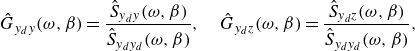 \begin{equation} {\hat {G}}_{y_dy}(\omega, \beta ) = \frac {{\hat {S}}_{y_dy}(\omega, \beta )}{{\hat {S}}_{y_dy_d}(\omega, \beta )}, \quad {\hat {G}}_{y_dz}(\omega, \beta ) = \frac {{\hat {S}}_{y_dz}(\omega, \beta )}{{\hat {S}}_{y_dy_d}(\omega, \beta )}, \end{equation}
with ${\hat {S}}_{lm}$
representing the cross-spectra between the time signals
${\hat {S}}_{lm}$
representing the cross-spectra between the time signals $l$
and
$l$
and $m$
, and the hat indicates that the quantities are in the frequency domain. Note that, due to the periodicity along the spanwise coordinate, the transfer functions are dependent on the spanwise wavenumber
$m$
, and the hat indicates that the quantities are in the frequency domain. Note that, due to the periodicity along the spanwise coordinate, the transfer functions are dependent on the spanwise wavenumber $\beta$
as well, where the discretisation is given by the discrete number of sensors. The time frequency part of the spectra,
$\beta$
as well, where the discretisation is given by the discrete number of sensors. The time frequency part of the spectra, $\omega$
, is computed by means of ensemble average (Bendat & Piersol Reference Bendat and Piersol2011), by using 28 batches with 75 % of overlap. The impulse response is finally retrieved by taking the inverse Fourier transform of the transfer functions in (3.9), referred to as
$\omega$
, is computed by means of ensemble average (Bendat & Piersol Reference Bendat and Piersol2011), by using 28 batches with 75 % of overlap. The impulse response is finally retrieved by taking the inverse Fourier transform of the transfer functions in (3.9), referred to as $g_{dy}(t,k)$
and
$g_{dy}(t,k)$
and $g_{dz}(t,k)$
. In this case, it is also worth noting that the way to estimate the signals
$g_{dz}(t,k)$
. In this case, it is also worth noting that the way to estimate the signals $\mathbf{y}$
and
$\mathbf{y}$
and $\mathbf{z}$
using the transfer functions
$\mathbf{z}$
using the transfer functions
 \begin{equation} {\hat {y}} = {\hat {G}}_{y_dy} {\hat {y}}_d, \quad \hat {z} = {\hat {G}}_{y_dz} {\hat {y}}_d, \end{equation}
correspond to double convolutions in physical space. In terms of the impulse response, this means that we have to repeat and translate $g_{y_dy}$
and
$g_{y_dy}$
and $g_{y_dz}$
along the span to obtain the response in time of the output
$g_{y_dz}$
along the span to obtain the response in time of the output $\textbf{y}$
and
$\textbf{y}$
and $\textbf{z}$
for each of the
$\textbf{z}$
for each of the $N_{y_d}$
sensors.
$N_{y_d}$
sensors.
4. Results
4.1. Reduced-order model and control kernel
With the methods described in § 3.1 and § 3.2 we can now obtain the control kernel as in (3.8). Figure 7 shows the time signal of one of the sensors for the uncontrolled case with $Tu=0.5\,\%$
, where we indicate the extent of the signal that is used to obtain the transfer functions in (3.9), and also the extent of the signal where the controller is tested in the simulations.
$Tu=0.5\,\%$
, where we indicate the extent of the signal that is used to obtain the transfer functions in (3.9), and also the extent of the signal where the controller is tested in the simulations.
Signal corresponding to one sensor for uncontrolled case, showing the extent of the signal used for design and testing the controller.

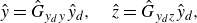
Figure 8 shows the singular values of the Hankel matrix $H_0$
with the threshold used to build the ROM for the case
$H_0$
with the threshold used to build the ROM for the case $Tu=0.5\,\%$
, resulting in a ROM of order
$Tu=0.5\,\%$
, resulting in a ROM of order $N=298$
. It also includes the comparison between the original impulse responses and the ones obtained from the ROM, where it can be seen that a good reconstruction is obtained. Due to periodicity along the span and the use of identical devices, these plots are shown as a function of the spacing
$N=298$
. It also includes the comparison between the original impulse responses and the ones obtained from the ROM, where it can be seen that a good reconstruction is obtained. Due to periodicity along the span and the use of identical devices, these plots are shown as a function of the spacing $\Delta x_3$
between one single input to the elements of the row of outputs downstream.
$\Delta x_3$
between one single input to the elements of the row of outputs downstream.
Comparison of original impulse responses ( $\color {black}-$
) and the ones from the ROM (
$\color {black}-$
) and the ones from the ROM ( $\color {red}-\color {red}-$
), corresponding to
$\color {red}-\color {red}-$
), corresponding to $\mathbf{d}\to\mathbf{y}$
(panel (b)),
$\mathbf{d}\to\mathbf{y}$
(panel (b)), $ \mathbf{d}\to\mathbf{z}$
(panel (c)), and
$ \mathbf{d}\to\mathbf{z}$
(panel (c)), and $\mathbf{u}\to\mathbf{z}$
(panel (c)). Panel (a) shows the singular values of the Hankel matrix and the threshold to build the ROM.
$\mathbf{u}\to\mathbf{z}$
(panel (c)). Panel (a) shows the singular values of the Hankel matrix and the threshold to build the ROM.
With the ROM, it is possible now to design the LQG. To solve the Riccati equations, (3.3) and (3.6), we start by defining the weight and covariance matrices as $\textbf{R}=R\textbf{I}_{N_u}$
,
$\textbf{R}=R\textbf{I}_{N_u}$
, $\textbf{Q}=Q\textbf{I}_{N_d}$
,
$\textbf{Q}=Q\textbf{I}_{N_d}$
, $\textbf{V}_n=v_n\textbf{I}_{N_y}$
and
$\textbf{V}_n=v_n\textbf{I}_{N_y}$
and $\textbf{V}_d=v_d\textbf{I}_{N_d}$
, with
$\textbf{V}_d=v_d\textbf{I}_{N_d}$
, with $\textbf{I}_m$
the identity matrix of size
$\textbf{I}_m$
the identity matrix of size $m$
and
$m$
and $R$
,
$R$
, $Q$
,
$Q$
, $v_n$
,
$v_n$
, $v_d$
scalar quantities. The final selection of these scalars is through trial and error by evaluating the performance of the ROM in minimising the output
$v_d$
scalar quantities. The final selection of these scalars is through trial and error by evaluating the performance of the ROM in minimising the output $\textbf{z}$
in the design data. Here, a performance index is defined as
$\textbf{z}$
in the design data. Here, a performance index is defined as
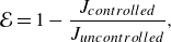 \begin{equation} \mathcal{E} = 1 - \frac {J_{{controlled}}}{J_{{uncontrolled}}}, \end{equation}
with
 \begin{equation} J = \frac {1}{N_zT} \int \limits _{0}^{T} \textbf{z}(t)^\textsf{T}\textbf{z}(t) \textrm{d}t, \end{equation}
which represents the mean square value of the output at the objective function location. The scalars $R$
,
$R$
, $Q$
,
$Q$
, $v_n$
and
$v_n$
and $v_d$
are evaluated as the ratios
$v_d$
are evaluated as the ratios $R/Q$
and
$R/Q$
and $v_n/v_d$
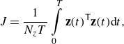
, and the performance of the kernels on the ROM for different ratios combinations are presented in figure 9, with the colours representing the values of (4.1). The control kernels are finally selected considering the parameter combination for which the ROM reaches the maximum performance in figure 9, where only the design data were used. Note that in figure 9 the parameter combinations leading to maximum performance are different among the cases, and while the underlying reasons were not investigated in detail, this behaviour can be attributed to the use of sensors and actuators of different sizes for each case. The kernels for the different cases under study are shown in figure 10. Despite some differences among the kernels, they all share some similarities. For instance, most of the weight is put into the sensor
$v_n/v_d$
, and the performance of the kernels on the ROM for different ratios combinations are presented in figure 9, with the colours representing the values of (4.1). The control kernels are finally selected considering the parameter combination for which the ROM reaches the maximum performance in figure 9, where only the design data were used. Note that in figure 9 the parameter combinations leading to maximum performance are different among the cases, and while the underlying reasons were not investigated in detail, this behaviour can be attributed to the use of sensors and actuators of different sizes for each case. The kernels for the different cases under study are shown in figure 10. Despite some differences among the kernels, they all share some similarities. For instance, most of the weight is put into the sensor $y$
at the same spanwise position
$y$
at the same spanwise position $\Delta x_3=0$
. Also, in all cases, the kernel presents the highest values around
$\Delta x_3=0$
. Also, in all cases, the kernel presents the highest values around $t=0$
to then decay rapidly towards zero. One of the main implications of this behaviour in our implementation is that the lower limit of the integral in (3.8) is replaced to
$t=0$
to then decay rapidly towards zero. One of the main implications of this behaviour in our implementation is that the lower limit of the integral in (3.8) is replaced to $ t-0.3$
. This is done to get a faster computation of the actuation signal, and justified by the fact that the convolution will render zero values for larger time lags.
$ t-0.3$
. This is done to get a faster computation of the actuation signal, and justified by the fact that the convolution will render zero values for larger time lags.
Performance of the ROM as in (4.1) for different weight and covariance ratio combinations.
Control kernels for the different cases as a function of time and the spanwise distance $\Delta x_3$
from the input
$\Delta x_3$
from the input $u_k$
to the outputs
$u_k$
to the outputs $\textbf{y}$
.
$\textbf{y}$
.
4.2. Control performance
The final control kernel designs presented in figure 10 are implemented and evaluated in the DNS considering only the time span of the test data, which was not used during the controller design. The use of numerical simulations allows us to have a full restart of the flow fields, being able to contrast the controlled and uncontrolled simulations at the exact same time and conditions.
We start by presenting the performance of the controller in the DNS simulations, where the focus is on three quantities of interest. The first quantity corresponds to the output time signal at the objective function location. The second quantity is disturbance attenuation in the boundary layer. And the last one corresponds to transition delay.
The results for the performance index using (4.1) are presented in table 2, where the values from the ROM and the DNS are included. We can observe that, despite small differences, the ROM predicts reasonably well the performance of the controller in the DNS in the test data. The time series of the mean square signal, along the spanwise direction, are presented in figure 11. From this set of plots and the results shown in table 2, we can conclude that all the controllers are effective in minimising the output at the objective function location. In particular, for the cases with $Tu=2.5\,\%$
the best performance is achieved for the controller corresponding to
$Tu=2.5\,\%$
the best performance is achieved for the controller corresponding to $N_{I/O}=20$
. This could be explained by the role of the actuator in generating wider structures along the span, as can be seen in figure 6, and it is therefore more effective in damping the energetic low wavenumbers in the flow. However, a more detailed comparison between the cases in table 2 is not very straightforward, due to the fact that the sensors are different in each case, measuring the average of the skin friction over the number-dependent sensor size. Therefore, the main point to emphasise from table 2 is that the controllers keeping their performance in the simulations suggests that the control laws are robust enough to act on a new data set, and also to account for differences between the ROM and the actual system.
$N_{I/O}=20$
. This could be explained by the role of the actuator in generating wider structures along the span, as can be seen in figure 6, and it is therefore more effective in damping the energetic low wavenumbers in the flow. However, a more detailed comparison between the cases in table 2 is not very straightforward, due to the fact that the sensors are different in each case, measuring the average of the skin friction over the number-dependent sensor size. Therefore, the main point to emphasise from table 2 is that the controllers keeping their performance in the simulations suggests that the control laws are robust enough to act on a new data set, and also to account for differences between the ROM and the actual system.
Controller performance, as in (4.1), for the different cases.
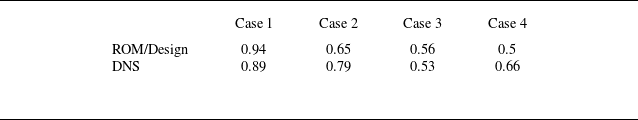
Mean square of the sensors measurements at the objective function location, with the red and black lines showing the uncontrolled and controlled simulations, respectively.
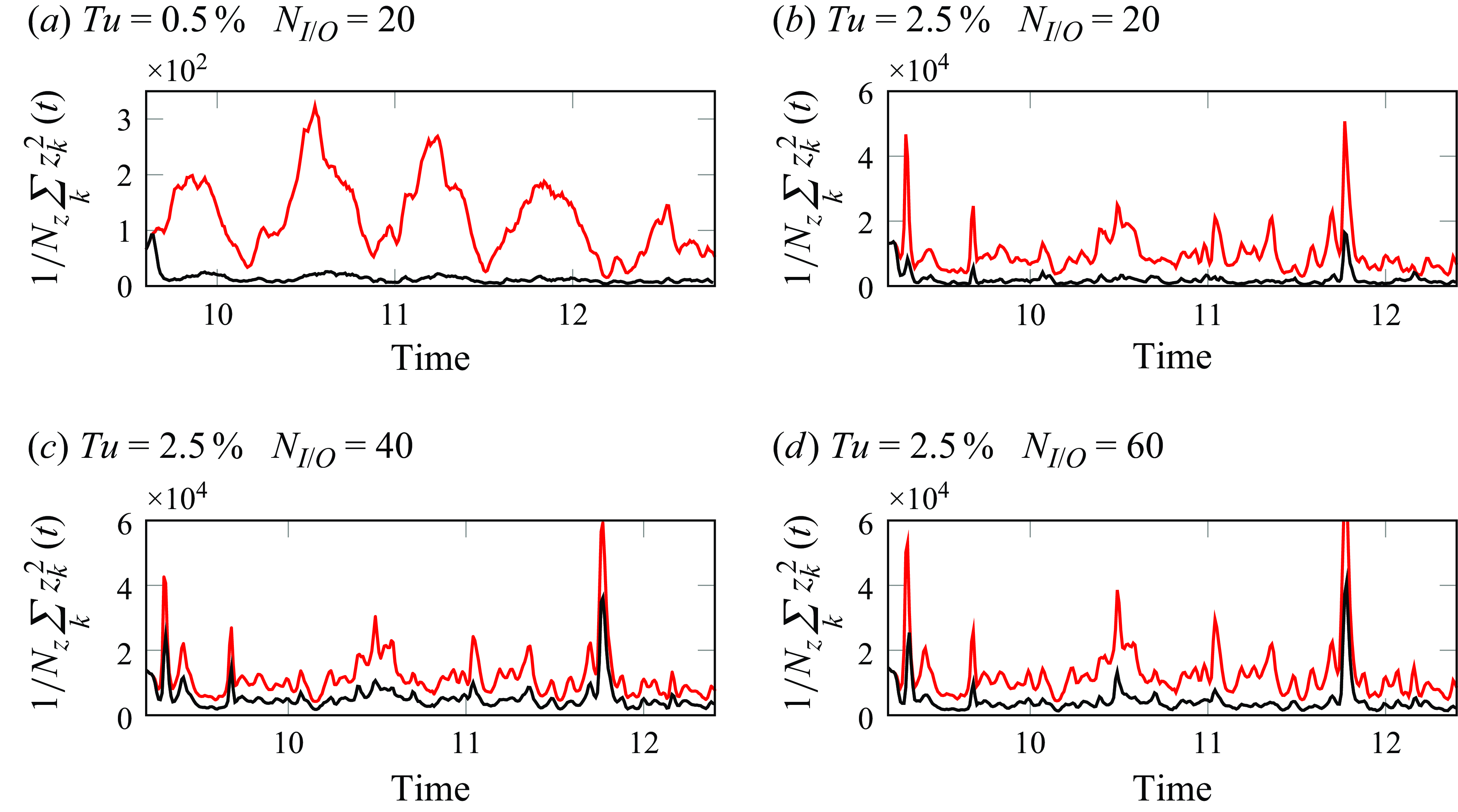
After corroborating that the controller is minimising the objective that it was designed for, we can inspect the effect that it has on the disturbances inside the boundary layer. Since the boundary layer is populated by streamwise streaks of different scales, as is the case of boundary layers forced by FST, we naturally choose the root mean square (r.m.s.) of the streamwise velocity as a first metric of interest to analyse. Figure 12 shows the maximum r.m.s. of the streamwise velocity along the chord for all the cases, noting that statistics were computed after a $\Delta T=0.4$
in order to allow the effect of the controller to reach the end of the domain. From panel (a), showing the case with
$\Delta T=0.4$
in order to allow the effect of the controller to reach the end of the domain. From panel (a), showing the case with $Tu=0.5\,\%$
, we can see that the controller effectively damps the streaks inside the boundary layer, and, similarly to the results for optimal disturbances in Semeraro et al. (Reference Semeraro, Bagheri, Brandt and Henningson2011), its effects are sustained throughout the domain. This case,
$Tu=0.5\,\%$
, we can see that the controller effectively damps the streaks inside the boundary layer, and, similarly to the results for optimal disturbances in Semeraro et al. (Reference Semeraro, Bagheri, Brandt and Henningson2011), its effects are sustained throughout the domain. This case, $Tu=0.5\,\%$
, was indeed the first simulation that was run to check that the controller configuration was effective in attenuating streaks. The response of the boundary layer to these FST conditions is mostly linear (Faúndez Alarcón et al. Reference Faúndez Alarcón, Morra, Hanifi and Henningson2022b
), which can explain the good performance of the controller designed under linear assumptions.
$Tu=0.5\,\%$
, was indeed the first simulation that was run to check that the controller configuration was effective in attenuating streaks. The response of the boundary layer to these FST conditions is mostly linear (Faúndez Alarcón et al. Reference Faúndez Alarcón, Morra, Hanifi and Henningson2022b
), which can explain the good performance of the controller designed under linear assumptions.
Figure 12(b) shows the results for the cases with $Tu=2.5\,\%$
, a turbulence level where nonlinear interaction become non-negligible. Here, we observe a similar behaviour as the case with
$Tu=2.5\,\%$
, a turbulence level where nonlinear interaction become non-negligible. Here, we observe a similar behaviour as the case with $Tu=0.5\,\%$
, where a noticeable attenuation of the streaks at the objective function location is obtained for all controlled cases, being also sustained downstream but, in these cases, not until the end of the domain. This is further portrayed with the velocity profiles at different
$Tu=0.5\,\%$
, where a noticeable attenuation of the streaks at the objective function location is obtained for all controlled cases, being also sustained downstream but, in these cases, not until the end of the domain. This is further portrayed with the velocity profiles at different $x_1$
stations shown in figure 13. When comparing the amplitude of the three controlled cases at the objective function location, we can also observe some differences in terms of their performance. In this respect, we do not observe a one-to-one correspondence between the minimisation of the objective function and the damping of the disturbance inside the boundary layer, where, for the latter, the best performance is attained to the case
$x_1$
stations shown in figure 13. When comparing the amplitude of the three controlled cases at the objective function location, we can also observe some differences in terms of their performance. In this respect, we do not observe a one-to-one correspondence between the minimisation of the objective function and the damping of the disturbance inside the boundary layer, where, for the latter, the best performance is attained to the case $N_{I/O}=60$
instead.
$N_{I/O}=60$
instead.
Maximum $q_{s,rms}$
inside the boundary layer for uncontrolled and controlled simulations. The right plots show the same quantity but normalised by the corresponding uncontrolled case.
$q_{s,rms}$
inside the boundary layer for uncontrolled and controlled simulations. The right plots show the same quantity but normalised by the corresponding uncontrolled case.
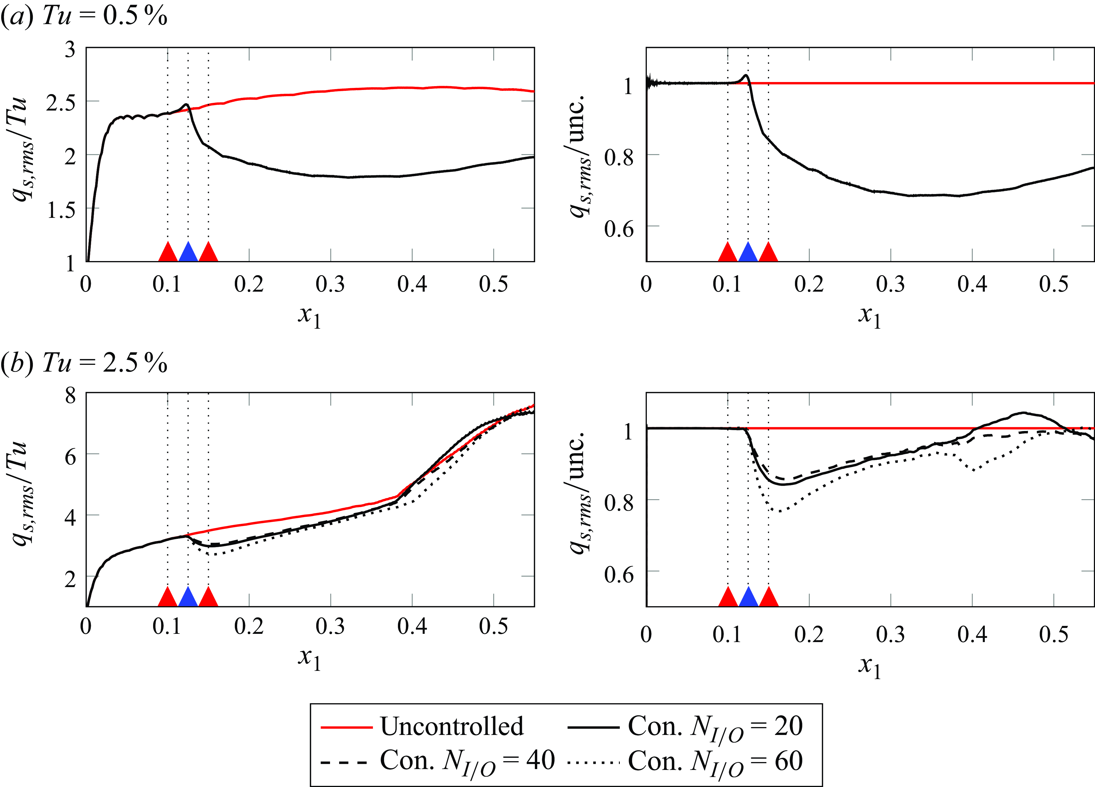
By looking downstream of the objective position, around $x_1\approx 0.4$
, we see an abrupt increment of the r.m.s. values, which is an indication of transition to a fully turbulent boundary layer. From this, it is possible to point out some interesting observations. First, even though the cases
$x_1\approx 0.4$
, we see an abrupt increment of the r.m.s. values, which is an indication of transition to a fully turbulent boundary layer. From this, it is possible to point out some interesting observations. First, even though the cases $N_{I/O}=20$
and
$N_{I/O}=20$
and $N_{I/O}=40$
sustain a lower disturbance level downstream of the objective compared with the uncontrolled case, around
$N_{I/O}=40$
sustain a lower disturbance level downstream of the objective compared with the uncontrolled case, around $x_1\approx 0.4$
they recover the level of the uncontrolled case with a slight better performance for case
$x_1\approx 0.4$
they recover the level of the uncontrolled case with a slight better performance for case $N_{I/O}=40$
. Interestingly, this recovery of the disturbance level towards the uncontrolled case has been observed experimentally in the work by Lundell (Reference Lundell2007). Secondly, the only case that shows a significant delay in the rapid rise of
$N_{I/O}=40$
. Interestingly, this recovery of the disturbance level towards the uncontrolled case has been observed experimentally in the work by Lundell (Reference Lundell2007). Secondly, the only case that shows a significant delay in the rapid rise of $q_{s,rms}$
is the one corresponding to
$q_{s,rms}$
is the one corresponding to $N_{I/O}=60$
. This is more clearly seen when looking at the r.m.s. streamwise velocity profiles at
$N_{I/O}=60$
. This is more clearly seen when looking at the r.m.s. streamwise velocity profiles at $x_1=0.4$
in figure 13, where only the case
$x_1=0.4$
in figure 13, where only the case $N_{I/O}=60$
shows a distinctive shape with respect to the uncontrolled case. While this could be attributed to the larger reduction at the objective function location, such a conclusion would contradict the behaviour observed in the other two cases, which takes us to the last point. The better performance of
$N_{I/O}=60$
shows a distinctive shape with respect to the uncontrolled case. While this could be attributed to the larger reduction at the objective function location, such a conclusion would contradict the behaviour observed in the other two cases, which takes us to the last point. The better performance of $N_{I/O}=20$
with respect to
$N_{I/O}=20$
with respect to $N_{I/O}=40$
in both minimising the objective function and the disturbance level at the objective position, does not translate into a better performance in terms of delaying the rapid growth of the r.m.s. downstream. On the contrary,
$N_{I/O}=40$
in both minimising the objective function and the disturbance level at the objective position, does not translate into a better performance in terms of delaying the rapid growth of the r.m.s. downstream. On the contrary, $N_{I/O}=40$
shows a better performance in this regard, which is more clear when observing the friction coefficient in figure 14. Moreover, when contrasting the three controlled cases at
$N_{I/O}=40$
shows a better performance in this regard, which is more clear when observing the friction coefficient in figure 14. Moreover, when contrasting the three controlled cases at $x_1=0.3$
in figure 13, they all exhibit a similar reduction, but at the next station
$x_1=0.3$
in figure 13, they all exhibit a similar reduction, but at the next station $x_1=0.4$
this similarity is not maintained, with
$x_1=0.4$
this similarity is not maintained, with $N_{I/O}=60$
clearly outperforming the other two cases.
$N_{I/O}=60$
clearly outperforming the other two cases.
Streamwise r.m.s. profiles at different streamwise stations $x_1$
. Lines as in figure 12.
$x_1$
. Lines as in figure 12.
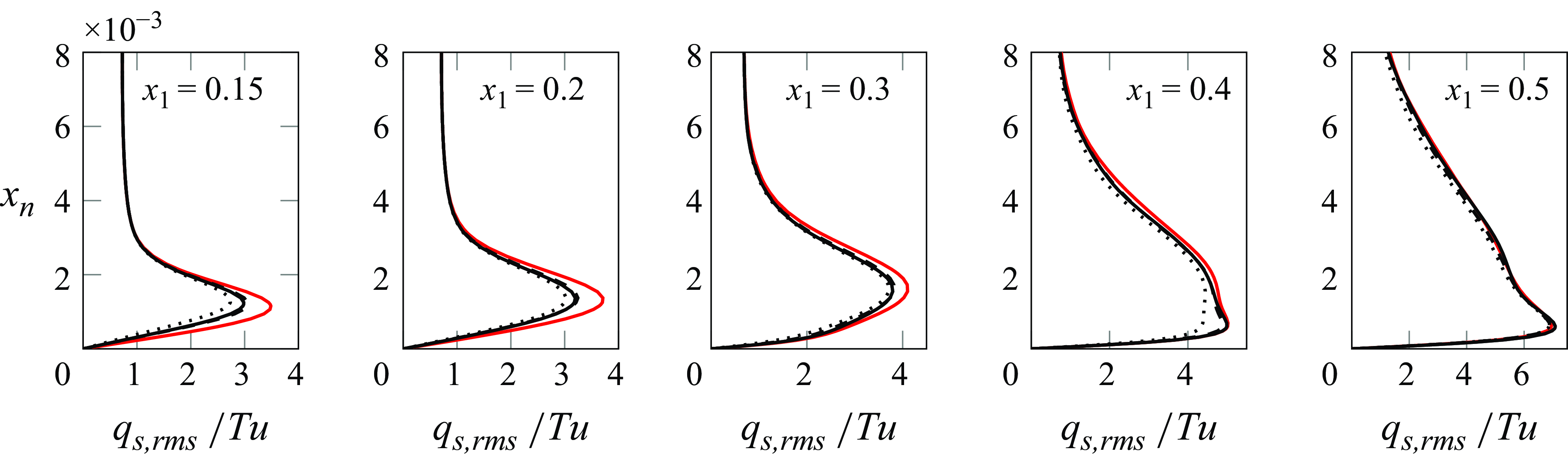
Before providing an explanation regarding the different behaviours of the controlled cases downstream of the objective function location, some remarks on the friction coefficient shown in figure 14 are provided. This is arguably the most important quantity for engineering applications, where lower values are generally sought for energy savings. In this context, only the case $N_{I/O}=60$
presents a noticeable reduction with respect to the uncontrolled case. Besides, the case
$N_{I/O}=60$
presents a noticeable reduction with respect to the uncontrolled case. Besides, the case $N_{I/O}=20$
has even higher values than the uncontrolled case at the end of the domain, which would make it unsuitable for any efforts regarding transition delay. Note also that at the actuator’s position, the cases
$N_{I/O}=20$
has even higher values than the uncontrolled case at the end of the domain, which would make it unsuitable for any efforts regarding transition delay. Note also that at the actuator’s position, the cases $N_{I/O}=20$
and
$N_{I/O}=20$
and $N_{I/O}=40$
show a crest and a valley which can be attributed to the lower actuation penalisation, as was shown in table 1 for the ratio
$N_{I/O}=40$
show a crest and a valley which can be attributed to the lower actuation penalisation, as was shown in table 1 for the ratio $R/Q$
.
$R/Q$
.
Friction coefficient for cases with $Tu=2.5\,\%$
, with the right plot showing the same quantity but normalised by the uncontrolled cased. Lines as in figure 12.
$Tu=2.5\,\%$
, with the right plot showing the same quantity but normalised by the uncontrolled cased. Lines as in figure 12.
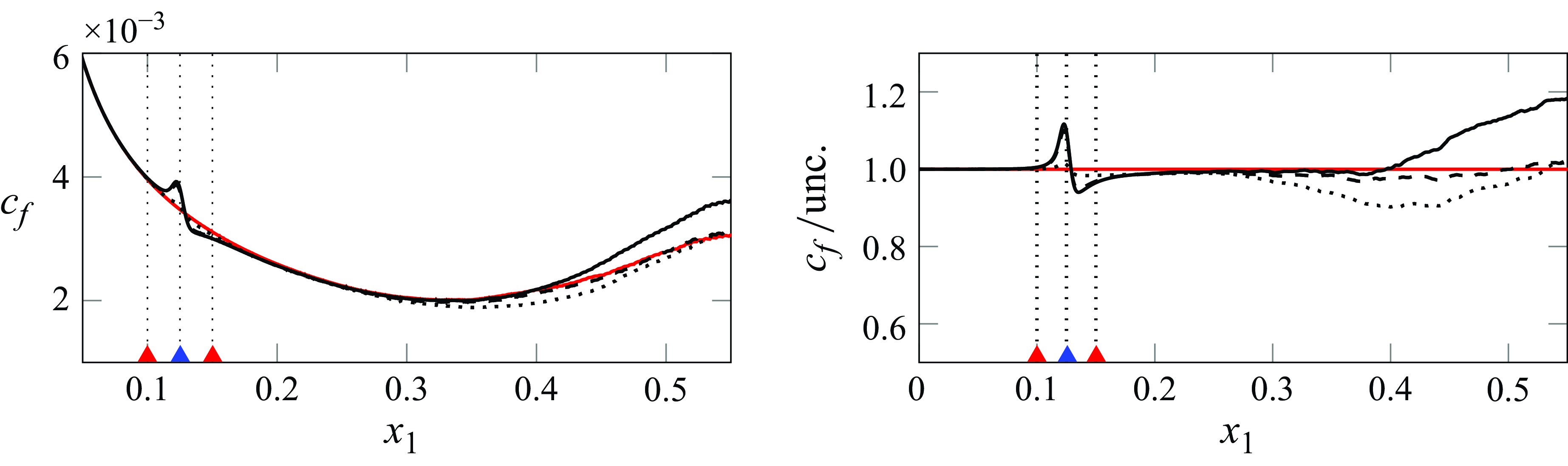
4.3. Turbulent spots
The results from the previous section show an intricate situation, where the reduction in the disturbance inside the boundary layer does not necessarily reflect on a better performance in terms of transition delay. In any case, a better performance is found for the controller corresponding to $N{I/O}=60$
when contrasted to the other two, and the purpose of this section is to shed some light on the causes behind this.
$N{I/O}=60$
when contrasted to the other two, and the purpose of this section is to shed some light on the causes behind this.
The motivation to act on the streaks and reduce their amplitude comes from the reasoning that these structures will grow and breakdown downstream, forming turbulent spots which will subsequently merge and create a fully turbulent boundary layer. This was, for instance, the result in the controlled case in Morra et al. (Reference Morra, Sasaki, Hanifi, Cavalieri and Henningson2019), where the nucleation of turbulent spots when the control was on took place downstream with respect to the uncontrolled case. In the present investigation, a similar behaviour can be observed for the case $N_{I/O}=60$
. To illustrate this, figure 15 shows the streamwise shear for the cases
$N_{I/O}=60$
. To illustrate this, figure 15 shows the streamwise shear for the cases $Tu=2.5\,\%$
at the same time instant, which can be recognised by comparing the contours of the different cases upstream of the actuation. At this time instant, a turbulent spot is seen in the uncontrolled case, and almost the same turbulent spot is observed in the cases
$Tu=2.5\,\%$
at the same time instant, which can be recognised by comparing the contours of the different cases upstream of the actuation. At this time instant, a turbulent spot is seen in the uncontrolled case, and almost the same turbulent spot is observed in the cases $N_{I/O}=20$
and
$N_{I/O}=20$
and $N_{I/O}=40$
. However, for the case
$N_{I/O}=40$
. However, for the case $N_{I/O}=60$
, only initial traces of it, corresponding to short wavelength streamwise modulation, can be noticed.
$N_{I/O}=60$
, only initial traces of it, corresponding to short wavelength streamwise modulation, can be noticed.
Streamwise shear at the same time instant $t=10.39$
for simulations corresponding to
$t=10.39$
for simulations corresponding to $Tu=2.5\,\%$
. The contours in the different plots share the same range for better comparison.
$Tu=2.5\,\%$
. The contours in the different plots share the same range for better comparison.
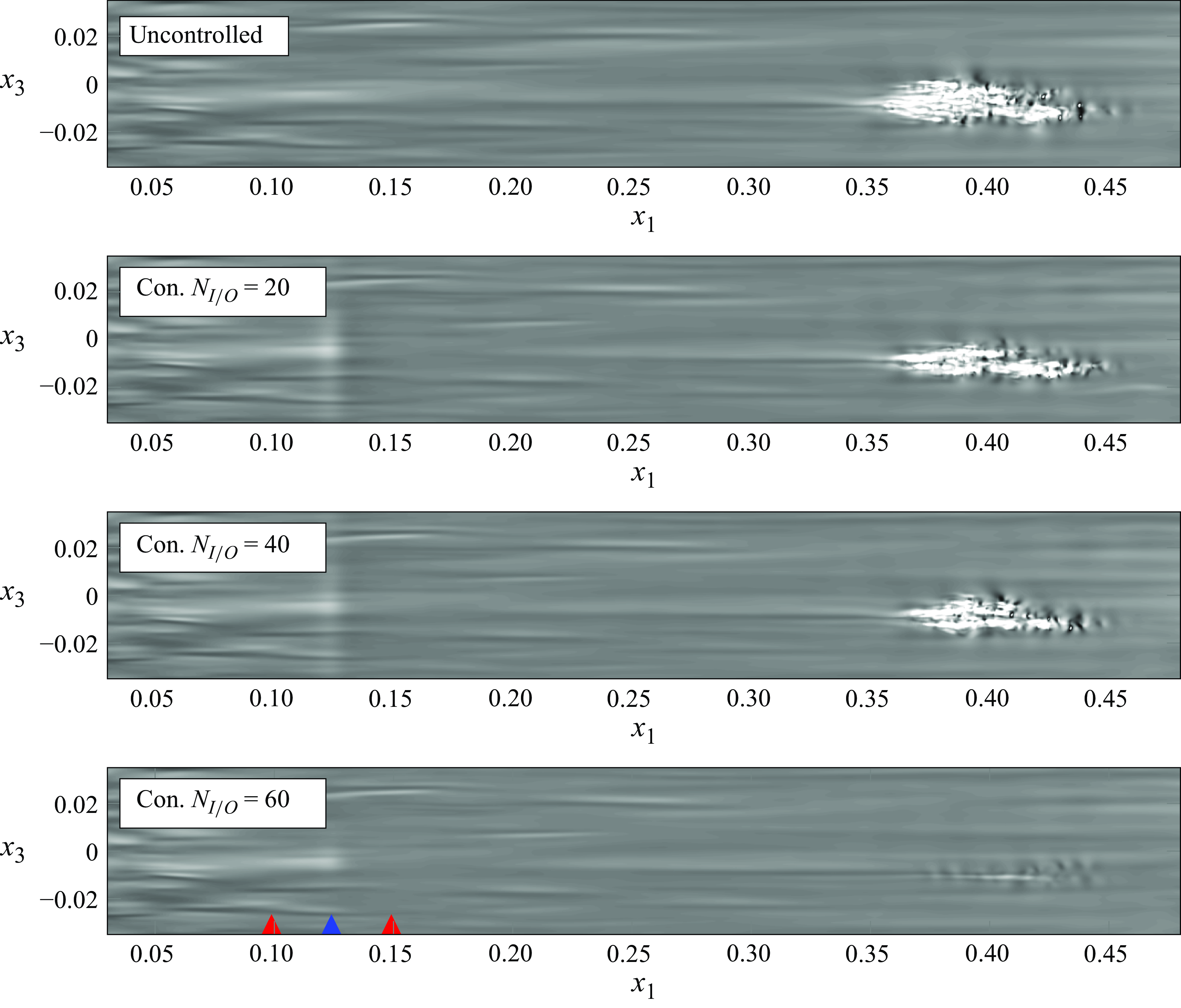
Figure 16 includes the time–space diagrams of the streamwise shear for the four cases, all of which are taken at the same spanwise position $x_3=-0.01$
. In these plots, we can see the nucleation and convection of turbulent spots, characterised by the high shear with the white contours levels. The turbulent spot labelled as (b) in figure 16 corresponds to the same event as the one depicted in figure 15, where the same situation can be appreciated: only the case
$x_3=-0.01$
. In these plots, we can see the nucleation and convection of turbulent spots, characterised by the high shear with the white contours levels. The turbulent spot labelled as (b) in figure 16 corresponds to the same event as the one depicted in figure 15, where the same situation can be appreciated: only the case $N_{I/O}=60$
is able to delay its nucleation with respect to the uncontrolled case. The spot (c) is observed in the three controlled simulations, but not in the uncontrolled one, which is of course an undesirable result. For the spots (d) and (e), the controller
$N_{I/O}=60$
is able to delay its nucleation with respect to the uncontrolled case. The spot (c) is observed in the three controlled simulations, but not in the uncontrolled one, which is of course an undesirable result. For the spots (d) and (e), the controller $N_{I/O}=60$
is effective in delaying their nucleation, while for the other two controlled cases no big differences with respect to the uncontrolled case are observed. Finally, spot (a) is effectively damped by controller
$N_{I/O}=60$
is effective in delaying their nucleation, while for the other two controlled cases no big differences with respect to the uncontrolled case are observed. Finally, spot (a) is effectively damped by controller $N_{I/O}=60$
within the domain.
$N_{I/O}=60$
within the domain.
Time–space diagram of the streamwise shear at spanwise position $x_3=-0.01$
. From left to right: uncontrolled, controlled
$x_3=-0.01$
. From left to right: uncontrolled, controlled $N_{I/O}=20$
,
$N_{I/O}=20$
, $N_{I/O}=40$
and
$N_{I/O}=40$
and $N_{I/O}=60$
.
$N_{I/O}=60$
.
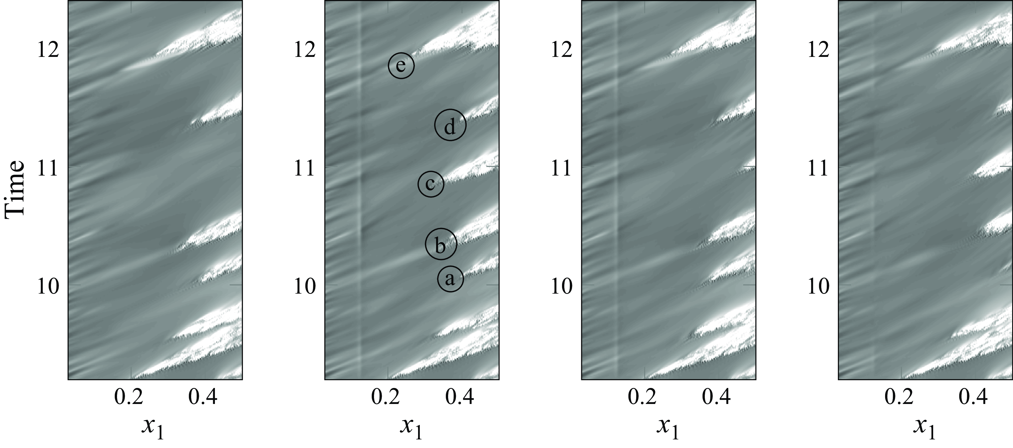
Figures 15 and 16 complement the statistical results presented in the previous section in figures 12 and 14, portraying a more comprehensive picture regarding the effect that the controllers have on the flow in terms of transition delay. In this respect, only the case $N_{I/O}=60$
seems to be effective in doing so by delaying the appearance of nucleation events. The underlying reason seems to be the scale of the streaks that become unstable and break down in this particular flow, and how effective the controller is in damping them. This explanation was already envisioned in our previous work Faúndez Alarcón et al. (Reference Faúndez Alarcón, Sasaki, Hanifi, Larsson and Henningson2022a
) by looking at consecutive snapshots and noting the spanwise spacing of the breaking streaks. In the present investigation, we strengthen this point through the use of local stability analysis.
$N_{I/O}=60$
seems to be effective in doing so by delaying the appearance of nucleation events. The underlying reason seems to be the scale of the streaks that become unstable and break down in this particular flow, and how effective the controller is in damping them. This explanation was already envisioned in our previous work Faúndez Alarcón et al. (Reference Faúndez Alarcón, Sasaki, Hanifi, Larsson and Henningson2022a
) by looking at consecutive snapshots and noting the spanwise spacing of the breaking streaks. In the present investigation, we strengthen this point through the use of local stability analysis.
The crucial role that streak secondary instabilities play in bypass transition has been shown, for instance, by Schlatter et al. (Reference Schlatter, Brandt, de Lange and Henningson2008), Hack & Zaki (Reference Hack and Zaki2014) and Faúndez Alarcón et al. (Reference Faúndez Alarcón, Cavalieri, Hanifi and Henningson2024). Therefore, the stability analysis in the pre-transitional part of flow can indicate the spanwise size of the streak involved in the nucleation of turbulent spots. On this basis, we perform local stability analysis in streamwise-normal planes located upstream and at previous time steps to turbulent spot nucleations. A temporal framework is adopted in the stability calculations, from which the output corresponds to a set of eigenfunctions whose complex eigenvalues dictate their stability. For completeness, the method is described in Appendix B.
Example of secondary instability before the nucleation event shown in figure 15. The top plot shows the full wing span, with the grey contours representing the streaks from the DNS and the red (negative) and blue (positive) contours the unstable mode from stability analysis. The bottom plots show, from left to right, the time–space evolution of the unstable mode (black dots) on top of the streamwise shear (grey contours), and zoomed views of the unstable mode at the first ( $x_1\approx 0.18$
) and last (
$x_1\approx 0.18$
) and last ( $x_1\approx 0.29$
) stations.
$x_1\approx 0.29$
) stations.
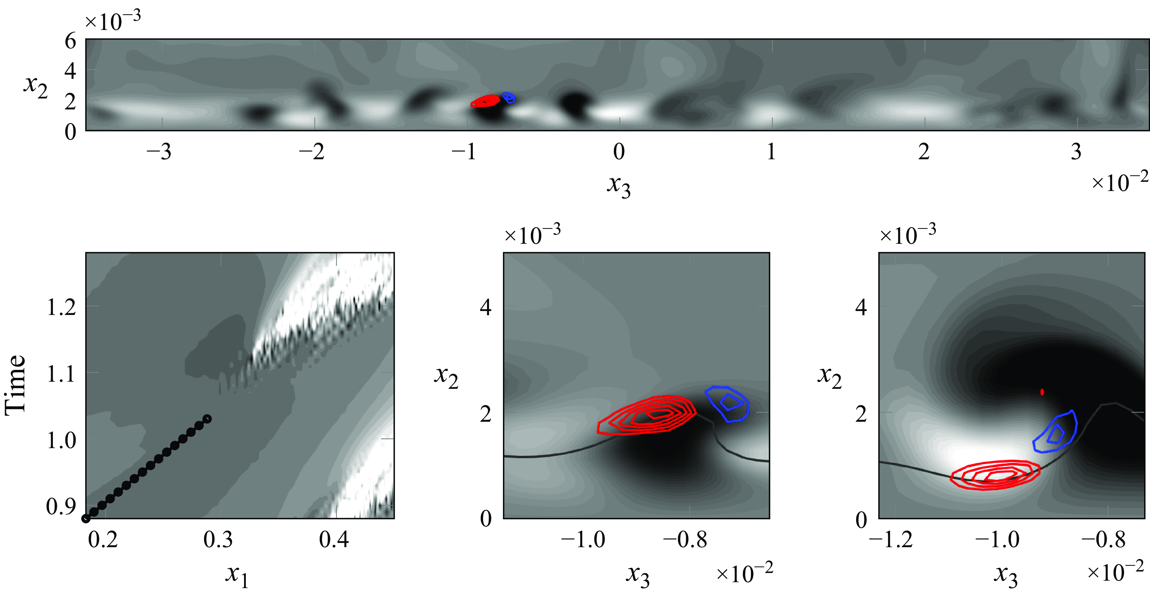
Figures 17 and 18 present two unstable modes appearing before the nucleation of turbulent spots. The stability calculations were performed on the uncontrolled case and considering a streamwise wavenumber $\alpha =800$
. From these two examples, it is clear that the unstable streaks in this flow configuration correspond to relatively short spanwise wavelength. Therefore, it is not surprising that the case
$\alpha =800$
. From these two examples, it is clear that the unstable streaks in this flow configuration correspond to relatively short spanwise wavelength. Therefore, it is not surprising that the case $N_{I/O}=20$
cannot perform well in terms of transition delay, given that the resolution given by the
$N_{I/O}=20$
cannot perform well in terms of transition delay, given that the resolution given by the $20$
sensors is not able to resolve such a short wavelength. By increasing the number of sensors, we increase the spanwise resolution and therefore start seeing some better performance in terms of transition delay. This can explain the better performance of controller
$20$
sensors is not able to resolve such a short wavelength. By increasing the number of sensors, we increase the spanwise resolution and therefore start seeing some better performance in terms of transition delay. This can explain the better performance of controller $N_{I/O}=60$
, and also the lack of correspondence between the performance in terms of disturbance damping at the objective function location and closer to the onset of transition, especially when comparing the cases
$N_{I/O}=60$
, and also the lack of correspondence between the performance in terms of disturbance damping at the objective function location and closer to the onset of transition, especially when comparing the cases $N_{I/O}=20$
and
$N_{I/O}=20$
and $N_{I/O}=40$
.
$N_{I/O}=40$
.
Another example of an unstable mode appearing before a nucleation event. Same description as caption in figure 17, but with first and last stations at $x_1\approx 0.19$
and
$x_1\approx 0.19$
and $x_1\approx 0.28$
, respectively.
$x_1\approx 0.28$
, respectively.
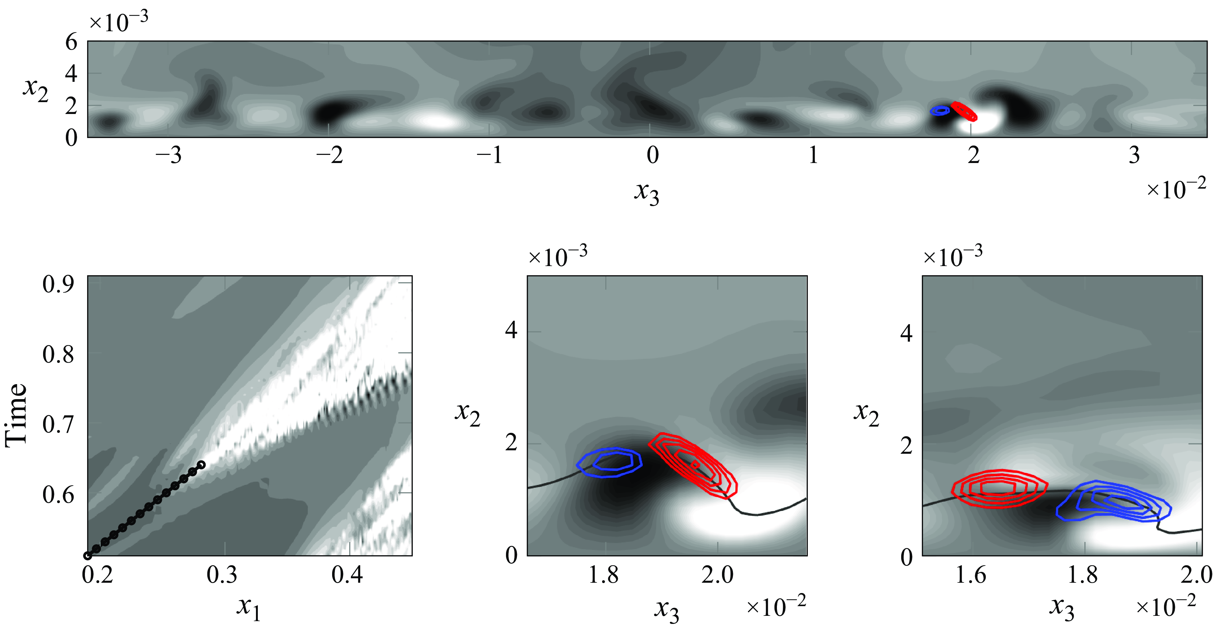
The effect of the different controllers over streaks with different spacings was corroborated by analysing the disturbance amplitude for different spanwise wavenumbers $\beta$
. This was done by computing the r.m.s. for each wavenumber in the frequency domain as
$\beta$
. This was done by computing the r.m.s. for each wavenumber in the frequency domain as
 \begin{equation} \hat {q}_{s,rms}(x_1,x_n,\beta ) = \frac {1}{n_{x_3}}\sqrt {\sum \limits _{\omega _k}\left |\frac {\hat {q}_s(\omega _k,x_1,x_n,\beta )}{n_t} \right |^2}, \end{equation}
where $\hat {q}_s$
is the double Fourier transform in time and along the homogeneous direction
$\hat {q}_s$
is the double Fourier transform in time and along the homogeneous direction $x_3$
, with
$x_3$
, with $n_t$
and
$n_t$
and $n_{x_3}$
the length of the time signal and the number of points along
$n_{x_3}$
the length of the time signal and the number of points along $x_3$
, respectively. Figure 19 shows the one-sided spectrum using (4.3) at the objective function location,
$x_3$
, respectively. Figure 19 shows the one-sided spectrum using (4.3) at the objective function location, $x_1=0.15$
, and for two wall-normal positions. From these two plots, it becomes clear that the controller
$x_1=0.15$
, and for two wall-normal positions. From these two plots, it becomes clear that the controller $N_{I/O}=20$
is very effective in damping the low spanwise wavenumbers, which are the most energetic waves in a statistical sense. Notably, it has actually the best reduction for the fundamental wavenumber
$N_{I/O}=20$
is very effective in damping the low spanwise wavenumbers, which are the most energetic waves in a statistical sense. Notably, it has actually the best reduction for the fundamental wavenumber $\beta _1$
. However, and given the number of sensors, its performance decreases towards higher wavenumbers, converging to the uncontrolled case curve after the 10th wavenumber. On the other hand, the cases with more sensors are able to damp these higher wavenumbers, in particular the case
$\beta _1$
. However, and given the number of sensors, its performance decreases towards higher wavenumbers, converging to the uncontrolled case curve after the 10th wavenumber. On the other hand, the cases with more sensors are able to damp these higher wavenumbers, in particular the case $N_{I/O}=60$
clearly outperforms the other two in this regard.
$N_{I/O}=60$
clearly outperforms the other two in this regard.
Distribution of the streamwise velocity r.m.s. along the spanwise wavenumbers, with lines as in figure 12. The time signals correspond to the cases with $Tu=2.5\,\%$
at the objective function location
$Tu=2.5\,\%$
at the objective function location $x_1=0.15$
, and the (a) and (b) plots represent the wall-normal positions
$x_1=0.15$
, and the (a) and (b) plots represent the wall-normal positions $x_n=0.5\delta ^*\approx 0.4\cdot 10^{-3}$
and
$x_n=0.5\delta ^*\approx 0.4\cdot 10^{-3}$
and $x_n=1.0\delta ^*\approx 0.8\cdot 10^{-3}$
, respectively. Here,
$x_n=1.0\delta ^*\approx 0.8\cdot 10^{-3}$
, respectively. Here, $\beta _1$
corresponds to the fundamental wavenumber given by the length of the domain.
$\beta _1$
corresponds to the fundamental wavenumber given by the length of the domain.
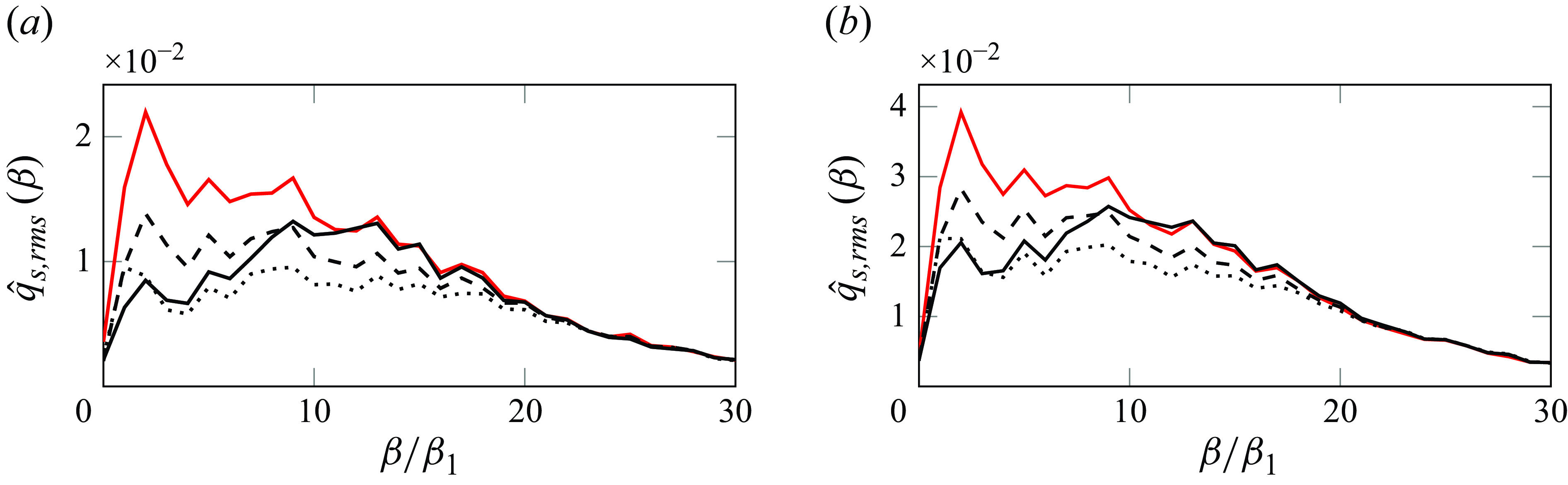
At first, the explanation regarding the controllers not being effective in damping the short span wavelengths appeared inconsistent with the results by Morra et al. (Reference Morra, Sasaki, Hanifi, Cavalieri and Henningson2019) and Sasaki et al. (Reference Sasaki, Morra, Cavalieri, Hanifi and Henningson2019), where the same procedure successfully delayed transition. In particular, Sasaki et al. (Reference Sasaki, Morra, Cavalieri, Hanifi and Henningson2019) showed that the use of optimised actuators, designed to efficiently damp the most energetic streaks in the flow field, outperformed the use of non-optimal actuator shapes. There is, however, a key difference between the present flow and the one used in the aforementioned work. In the latter, the breaking streaks are the most energetic as well. This observation comes from the comparison between the eigenvalues of the spectral proper orthogonal decomposition (SPOD) modes in Sasaki et al. (Reference Sasaki, Morra, Cavalieri, Hanifi and Henningson2019) (cf. figure 5), where the most energetic streaks are associated with the 3rd wavenumber, and the stability analysis of their flow field before a nucleation event. For the stability analysis, the data were kindly provided by the authors, and an example of an unstable mode before nucleation is shown in figure 20. By noticing that the figure comprises the full span of their simulations, we can see how the breaking, unstable, streak represents the 3rd wavenumber of the domain, and therefore it is also the most energetic one from the SPOD calculations. This can explain the performance differences between the Morra et al. (Reference Morra, Sasaki, Hanifi, Cavalieri and Henningson2019) and Sasaki et al. (Reference Sasaki, Morra, Cavalieri, Hanifi and Henningson2019) investigations and the present work. This situation, where breaking streaks are not necessarily the most energetic ones, together with the sporadic nucleation of turbulent spots, makes also challenging the design of optimal actuators targeting breaking streaks (Sasaki et al. Reference Sasaki, Morra, Cavalieri, Hanifi and Henningson2019), as it would require long time series to collect a significant amount of breaking events for their characterisation. One could expect, however, that a significant attenuation of the energetic structures would lead to weaker nonlinear interactions and thus a more pronounced effect regarding transition delay. One possible reason limiting this to happen is that, in this flow configuration, the nonlinear interactions responsible for generating the breaking streaks already took place upstream of actuation. Therefore, when the controller effectively damps those smaller scales as well (case 4) we start seeing a bigger impact when it comes to transition delay.
Unstable mode before a nucleation event in the case by Morra et al. (Reference Morra, Sasaki, Hanifi, Cavalieri and Henningson2019) and Sasaki et al. (Reference Sasaki, Morra, Cavalieri, Hanifi and Henningson2019). The plane is at $Re_x=3.5^{-5}$
, and the axis scaling corresponds to the one used in their work.
$Re_x=3.5^{-5}$
, and the axis scaling corresponds to the one used in their work.
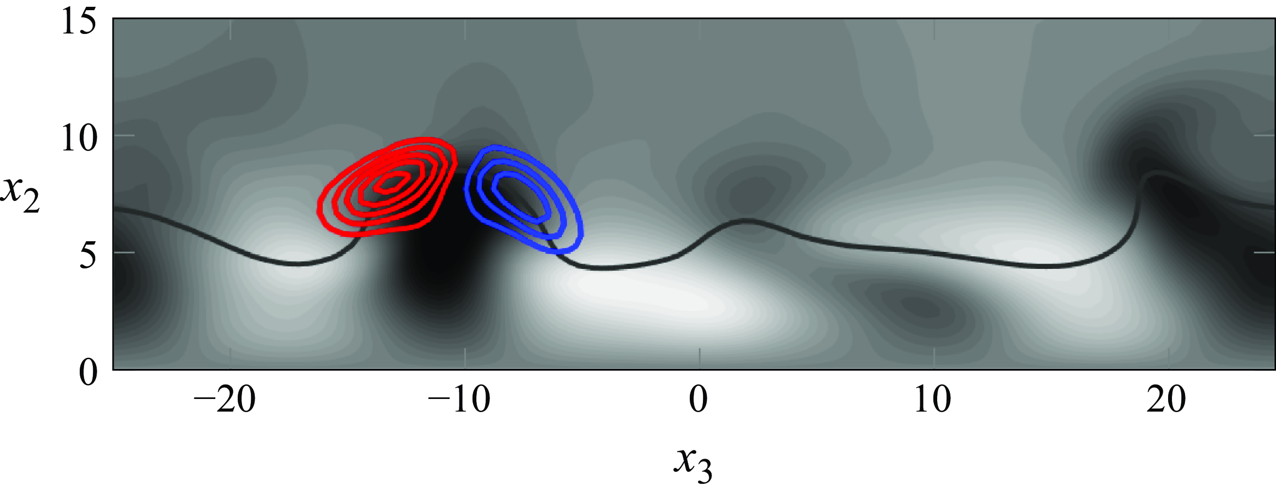
5. Conclusions
In this investigation, we have implemented an optimal controller to damp the disturbances in a wing boundary forced by FST using numerical simulations, considering two turbulence intensity levels and one integral length scale. The controller configuration is built from localised sensors and actuators placed in rows along the wing spanwise direction. The localised choice of devices is motivated by the commonly limitations encountered in experiments, where generally only wall information and actuation is possible. The control law is designed on a ROM, which is obtained from the input/output signals of the system only.
The design of the control law relied on a ROM, which was constructed using the ERA method. In this algorithm, the model is identified from the impulse responses of the system without the need of a priori knowledge of the operators. Due to the broadband nature of the incoming disturbances, computing their impulse responses is computationally demanding and unfeasible in experiments. Therefore, an extra row of dummy sensors is placed upstream of the control devices, where the transfer function between this row of sensors and the ones downstream is used as a proxy for the true impulse response of the disturbances. Once the impulse responses are collected, the ERA produces a model that reproduces the input/output relationships of the original system, with a state vector with size of just of the order of hundred.
The low dimensionality of the ROM makes the design of the LQG affordable, where, by adopting a feedforward configuration, the actuation signal is based only on upstream measurements. Once the controller is active, it is found that it effectively reduces the objective function not only in the ROM but also in the full numerical simulation. By imposing a low FST, where the dynamics of the system is nearly linear, we show that the controller is also effective in damping the streak amplitudes, and maintaining this reduction until the end of the domain. One of the implications of this is that the streamwise wall shear is a good surrogate measurement to be minimised when disturbance reduction is sought.
By increasing the turbulence intensity of the simulation, we assessed the linear control performance when nonlinear interactions become relevant. In this scenario, we analysed 3 different control configurations, by changing the number of sensors/actuators along the span. In all the cases, the objective function is minimised in the DNS accordingly to the ROM. Moreover, a noticeable disturbance reduction is achieved by all the controllers at the objective function location. Such reduction is maintained downstream, but different behaviours are observed in this regard. Here, only the case with the larger number of sensors presents a perceptible delay of the onset to transition, while the other two converge to the uncontrolled case at the transition onset. We argued that this is related to the effectiveness of the controllers in damping the streaks that will later break down, forming turbulent spots. In this flow configuration, they correspond to streaks with relatively short spanwise wavelength, which explains why increasing the number of sensors improves the performance. This recovery of the disturbance amplitude towards the uncontrolled case has also been observed experimentally in Lundell (Reference Lundell2007), where it was conjectured that this could either be the effect of optimal disturbances growing again downstream (Högberg & Henningson Reference Högberg and Henningson2002), or of new streaks entering from the side or generated by the free stream. Our results provide an alternative explanation for this behaviour, that can be nonetheless related to new nonlinearly generated streaks due to energy propagation. This energy transfer, from low to high wavenumbers through the $\beta$
-cascade (Henningson et al. Reference Henningson, Lundbladh and Johansson1993), is able to initiate streaks that can experience maximum growth at upstream positions with respect to their predecessors, and therefore become unstable before. This idea has been proposed in Faúndez Alarcón et al. (Reference Faúndez Alarcón, Cavalieri, Hanifi and Henningson2025), where different DNS were analysed.
$\beta$
-cascade (Henningson et al. Reference Henningson, Lundbladh and Johansson1993), is able to initiate streaks that can experience maximum growth at upstream positions with respect to their predecessors, and therefore become unstable before. This idea has been proposed in Faúndez Alarcón et al. (Reference Faúndez Alarcón, Cavalieri, Hanifi and Henningson2025), where different DNS were analysed.
In this work, we have followed the procedure developed by Morra et al. (Reference Morra, Sasaki, Hanifi, Cavalieri and Henningson2019) and Sasaki et al. (Reference Sasaki, Morra, Cavalieri, Hanifi and Henningson2019), where they successfully delayed transition in a flat plate. When contrasting their work with our results, similar performances in terms of the disturbance damping at the objective function location are obtained, but with different outcomes downstream at the transition onset. We provide an explanation for this apparent discrepancy based on the stability of the different flow fields. In this context, we show that the breaking streaks in Sasaki et al. (Reference Sasaki, Morra, Cavalieri, Hanifi and Henningson2019) correspond to the most energetic structures in the perturbation field, making their damping effective delay their breakdown. In the present flow case, the breaking streaks are associated with short spanwise wavelengths, which are not necessarily the most energetic disturbances at the objective function location. Therefore, the amplitude reduction at the objective function location does not necessarily translate into amplitude reduction of breaking streaks downstream. Consequently, our results suggest that, for effective transition delay, the controller should target the breaking streaks. While this might come as an obvious observation, one challenge is that they are not necessarily the most energetic ones where actuation is applied.
Several constraints have been considered to account for some of the limitations commonly encountered in experiments, such as localised sensing and actuation, and a design based on input/output data only. Moreover, the numerical simulations include the leading edge to properly resolve the penetration of the free-stream disturbances into the boundary layer. Compared with similar previous numerical investigations, a larger integral length scale was selected to have a value closer to those typically found in grid-generated turbulence. Nevertheless, there are still some experimental aspects that were not addressed in the present work and could limit the controller implementation. For example, regarding the actuation signal, no bounds were imposed to avoid unfeasible values or constraints for real-time calculations. Also, while the actuators had localised support acting only in the wall-normal direction, no attempt was made to resemble the shape of a real device. Another relevant aspect is the robustness of the controller. Although the controller performance was tested with new data, no studies were carried out to evaluate possible performance deviations under different conditions, such as free-stream velocity, angles of attack or different disturbance environments.
Acknowledgements.
The computations were performed on resources provided by The National Academic Infrastructure for Supercomputing in Sweden (NAISS) at PDC and NSC.
Funding.
This work was funded by Vinnova through the NFFP project LaFloDes (grant number 2019-05369); the European Research Council (grant agreement 694452-TRANSEP-ERC-2015-AdG); and the Swedish e-Science Research Centre (SeRC).
Declaration of interests.
The authors report no conflict of interest.
Appendix A. Eigensystem realisation algorithm implementation
In this appendix, we include the steps followed to obtain the ROM from the ERA. These steps consist in
-
(i) Run the impulse responses of the system for $2N_t+2$
steps and store them in the form
$\{ {\textbf{Y}}_0,{\textbf{Y}}_1,\ldots, {\textbf{Y}}_{2N_t+2}\}$
. Here, the response of the
$N_y+N_z$
outputs from the
$N_u+N_d$
are stacked together in the
${\textbf{Y}}_i\in \mathbb{R}^{(N_y+N_z)\times (N_u+N_d)}$
matrices. Alternatively, and due to the linearity of the system, the same procedure could be done for each of the inputs of the system.
$2N_t+2$
steps and store them in the form
$\{ {\textbf{Y}}_0,{\textbf{Y}}_1,\ldots, {\textbf{Y}}_{2N_t+2}\}$
. Here, the response of the
$N_y+N_z$
outputs from the
$N_u+N_d$
are stacked together in the
${\textbf{Y}}_i\in \mathbb{R}^{(N_y+N_z)\times (N_u+N_d)}$
matrices. Alternatively, and due to the linearity of the system, the same procedure could be done for each of the inputs of the system. -
(ii) Assemble the block Hankel matrices
(A1)
\begin{equation} H_0= \begin{bmatrix} {\textbf{Y}}_{0} & {\textbf{Y}}_{1} & \cdots & {\textbf{Y}}_{N_t}\\ {\textbf{Y}}_{1} & {\textbf{Y}}_{2} & \cdots & {\textbf{Y}}_{N_t+1}\\ \vdots & \vdots & \ddots & \vdots \\ {\textbf{Y}}_{N_t} & {\textbf{Y}}_{N_t+1} &\cdots & {\textbf{Y}}_{2N_t+1} \end{bmatrix}, \qquad H_1= \begin{bmatrix} {\textbf{Y}}_{1} & {\textbf{Y}}_{2} & \cdots & {\textbf{Y}}_{N_t+1}\\ {\textbf{Y}}_{2} & {\textbf{Y}}_{3} & \cdots & {\textbf{Y}}_{N_t+2}\\ \vdots & \vdots & \ddots & \vdots \\ {\textbf{Y}}_{N_t+1} & {\textbf{Y}}_{N_t+2} &\cdots & {\textbf{Y}}_{2N_t+2} \end{bmatrix}. \end{equation}
-
(iii) Compute the SVD of
$H_0=U\Sigma V^*$
. After sorting the singular values in descending order, we get the truncated matrices
$U_r$
and
$V_r$
by taking their first
$r$
columns and
$\Sigma _r$
by taking its first
$r$
rows. -
(iv) The reduced matrices of the system (3.1) are obtained from
(A2a)
\begin{align} \textbf{T}_r &= \Sigma _r^{-1/2}U_r^*H_1V_r\Sigma _r^{-1/2}, \end{align}
(A2b)
\begin{align} \textbf{B}_{r} &= \text{the first $N_u+N_d$ columns of } \Sigma ^{1/2}V_r^*, \end{align}
(A2c)
\begin{align} \textbf{C}_{r} &= \text{the first $N_y+N_z$ rows of } U_r\Sigma ^{1/2}. \end{align}
The matrices
$\textbf{B}_{u,r}$
and
$\textbf{B}_{d,r}$
are taken as the first
$N_u$
and last
$N_d$
columns of
$\textbf{B}_r$
, respectively, and the matrices
$\textbf{C}_{y,r}$
and
$\textbf{C}_{z,r}$
as the first
$N_y$
and last
$N_z$
rows of
$\textbf{C}_r$
, respectively. The reduced version of
$\textbf{A}$
is obtained by solving the equation
$\textbf{T}_r = e^{\textbf{A}_r \varDelta t}$
.


Appendix B. Local stability analysis
To perform local stability analysis, the velocity and pressure flow fields are decomposed as
 \begin{align} \textbf{Q}(t,\textbf{x}) &= \textbf{Q}_{BF}(x_2,x_3) + \varepsilon \textbf{q}(t,\textbf{x}), \end{align}
 \begin{align} P(t,\textbf{x}) &= P_0(x_2,x_3) + \varepsilon p(t,\textbf{x}), \end{align}
with $\textbf{Q}_{BF}=(Q_1,Q_2,Q_3)^{\textsf{T}}$
representing in this case the streaky base flow and
$\textbf{Q}_{BF}=(Q_1,Q_2,Q_3)^{\textsf{T}}$
representing in this case the streaky base flow and $\textbf{q}$
the disturbance state function with amplitude
$\textbf{q}$
the disturbance state function with amplitude $\varepsilon \ll 1$
. Here, a homogeneous assumption is invoked for the base flow, which is taken as frozen planes at a given
$\varepsilon \ll 1$
. Here, a homogeneous assumption is invoked for the base flow, which is taken as frozen planes at a given $x_1$
streamwise position. By assuming a normal mode for the perturbation
$x_1$
streamwise position. By assuming a normal mode for the perturbation $\textbf{q}(\textbf{x}) = \hat {\textbf{q}}(x_2,x_3) \exp (i (\alpha x_1 + \omega t))$
, and similarly for the pressure perturbation, while neglecting the nonlinear terms, the following linearised system is obtained
$\textbf{q}(\textbf{x}) = \hat {\textbf{q}}(x_2,x_3) \exp (i (\alpha x_1 + \omega t))$
, and similarly for the pressure perturbation, while neglecting the nonlinear terms, the following linearised system is obtained
 \begin{align} &\left ( \mathcal{C}- \Delta \right ) \hat {q}_1 + \left ( \mathcal{D}_{x_2} Q_1\right ) \hat {q}_2 + \left (\mathcal{D}_{x_3} Q_1\right ) \hat {q}_3 + i\alpha \hat {p} = i\omega \hat {q}_1, \end{align}
 \begin{align} &\,\,\left ( \mathcal{C}- \Delta + \mathcal{D}_{x_2} Q_2 \right ) \hat {q}_2 + \left (\mathcal{D}_{x_3} Q_2 \right ) \hat {q}_3 + \mathcal{D}_{x_2} \hat {p} = i\omega \hat {q}_2, \end{align}
 \begin{align} &\,\,\left (\mathcal{D}_{x_2} Q_3 \right ) \hat {q}_2+\left ( \mathcal{C}- \Delta + \mathcal{D}_{x_3} Q_3 \right ) \hat {q}_3+ \mathcal{D}_{x_3} \hat {p} = i\omega \hat {q}_3, \end{align}
 \begin{align} &\qquad\qquad\qquad i \alpha \hat {q}_1 + \mathcal{D}_{x_2} \hat {q}_2 + \mathcal{D}_{x_3} \hat {q}_3 = 0, \end{align}
where $\mathcal{C}=Q_1 i\alpha + Q_2 \mathcal{D}_{x_2} + W\mathcal{D}_{x_3}$
,
$\mathcal{C}=Q_1 i\alpha + Q_2 \mathcal{D}_{x_2} + W\mathcal{D}_{x_3}$
, $\Delta =1/Re (-\alpha ^2+\mathcal{D}_{x_2}^2 + \mathcal{D}_{x_3}^2 )$
,
$\Delta =1/Re (-\alpha ^2+\mathcal{D}_{x_2}^2 + \mathcal{D}_{x_3}^2 )$
, $\mathcal{D}_{x_2}=\partial /\partial x_2$
and
$\mathcal{D}_{x_2}=\partial /\partial x_2$
and $\mathcal{D}_{x_3}=\partial /\partial x_3$
. Here, the streamwise wavenumber
$\mathcal{D}_{x_3}=\partial /\partial x_3$
. Here, the streamwise wavenumber $\alpha$
is a parameter, and
$\alpha$
is a parameter, and $\omega$
has a complex value whose real part represents the angular frequency and the imaginary part the temporal growth rate.The differential operators are constructed from a fourth-order finite difference scheme. For the boundary conditions, no slip is imposed at
$\omega$
has a complex value whose real part represents the angular frequency and the imaginary part the temporal growth rate.The differential operators are constructed from a fourth-order finite difference scheme. For the boundary conditions, no slip is imposed at $x_2=0$
, periodicity along the spanwise direction
$x_2=0$
, periodicity along the spanwise direction $x_3$
and zero velocity in the free stream. Since the right-hand side matrix in the generalised eigenvalue problem of the system (B2) is singular, a shift-and-invert Arnoldi algorithm is employed due to its fast convergence.
$x_3$
and zero velocity in the free stream. Since the right-hand side matrix in the generalised eigenvalue problem of the system (B2) is singular, a shift-and-invert Arnoldi algorithm is employed due to its fast convergence.


 Open access