


1. Introduction
With the arrival of COVID-19, most nations implemented non-pharmaceutical interventions (NPIs) to prevent disease spread including mandated mask-wearing, stay-at-home orders and social distancing. While there is solid evidence that such measures are effective in slowing the spread of the disease [Reference Prakash, Srivastava, Singh, Sharma and Jain37, Reference Sun, Lau, Yeoh, Chung, Leung, Yam and Hung43], public health experts quickly realised that the effectiveness was hampered by non-compliance with NPIs among a nontrivial portion of the population, and that this non-compliance had a nontrivial effect on the disease spread [Reference Binte Aamir, Ahmad Zaidi and Abbas8, Reference Costa, Vernal, Giavina-Bianchi, Mesquita Peres, dos Santos, Santos, Santos, Francisco, Satie, dal Secco, Pivetta Cora, dos santos, Duarte, Oliveira Bonfá, Perreira, Sabino, Segurado and Levin17, Reference Seale, Dyer, Abdi, Rahman, Sun, Qureshi, Dowell-Day, Sward and Islam39, Reference Shumway, Hopper, Tolman, Ferguson, Hubble, Patterson, Jensen and Delcea40]. Thus, it is important to develop mathematical models for epidemiology which incorporate these sort of human behavioural effects.
We model non-compliance with NPIs in a manner borrowed from social contagion theory [Reference Christakis and Fowler16, Reference Sooknanan and Comissiong42], which is the idea that human behaviours and emotions can “spread” much like a disease. Among other applications, social contagion theory has been successfully used to model alcohol and drug use [Reference Ali, Amialchuk and Dwyer2, Reference van den Ende, van der Maas, Epskamp and Lees46], spread of deleterious mental health conditions [Reference Eisenberg, Golberstein, Whitlock and Downs19], participation in violent and/or gang-related activity [Reference Bond and Bushman9, Reference Brantingham, Yuan and Herz11] and teenage sexual behaviour [Reference Rodgers, Rowe and Buster38]. Inspired by social contagion theory, [Reference Bongarti, Galvan, Hatcher, Lindstrom, Parkinson, Wang and Bertozzi10, Reference Parkinson and Wang34] consider a compartmental susceptible–infectious–recovered (SIR) type models, wherein parallel to the disease spread, non-compliance with NPIs spreads through the population and affects the dynamics of the disease. Compartmental modelling of epidemics using partial differential equations (PDE) to account for spatially heterogeneous disease spread is now commonplace [Reference Avila-Vales and Pérez3, Reference Deng18, Reference Gai, Iron and Kolokolnikov21, Reference Lei, Li and Zhao28, Reference Wang, Zhang and Teng48], though most such manuscripts do not incorporate human behaviour. One notable exception is the work of Berestycki et al. [Reference Berestycki, Desjardins, Heintz and Oury5, Reference Berestycki, Desjardins, Weitz and Oury6] where a compartmental ordinary differential equation (ODE) model is generalised by allowing the susceptible population and transmission rate to depend heterogeneously on a newly introduced variable, which describes the level of risk acceptance or aversion throughout the population. In doing so, they derive a reaction-diffusion system where the populations are spatially homogeneous, but diffusion occurs with respect to risk aversion variable. In this way, the authors of [Reference Berestycki, Desjardins, Heintz and Oury5, Reference Berestycki, Desjardins, Weitz and Oury6] are also modelling the simultaneous spread of a disease and human behaviour (which has a bearing on the spread of the disease), though in a manner which is different from that of [Reference Bongarti, Galvan, Hatcher, Lindstrom, Parkinson, Wang and Bertozzi10, Reference Parkinson and Wang34]. The authors of [Reference Chen, Espinoza, Chou, Gumel, Levin and Marathe15, Reference Pant, Safdar, Santillana and Gumel33] also consider non-compliance with NPIs, though their models are spatially homogeneous and involve simple linear transfer between the compliant and non-compliant populations, in contrast to the spatial heterogeneity and mass-action transfer between the two considered in [Reference Bongarti, Galvan, Hatcher, Lindstrom, Parkinson, Wang and Bertozzi10, Reference Parkinson and Wang34] and in this manuscript. Besides these, there are many other interesting extensions of the basic SIR model which employ ODE and PDE—for example, multi-group models which stratify the population by age, co-morbities or a variety of other factors [Reference Bajiya, Tripathi, Kakkar, Wang and Sun4, Reference Bichara and Iggidr7, Reference Feng, Huang and Castillo-Chavez20, Reference Wang, Pang and Liu47, Reference Yang and Mao50] and hybrid discrete-continuous models which pair ODE or PDE with an agent-based approach [Reference Ala’raj, Majdalawieh and Nizamuddin1, Reference Cantin, Silva and Banos12, Reference Ochab, Manfredi, Puszynski and d’Onofrio32]. However, as stated above, few have incorporated human behavioural concerns in PDE models for epidemiology.
In addition to incorporating spatial heterogeneity and non-compliance with NPIs into our model, we are interested in control of an epidemic by some hypothetical governing agency. That is, we would like to model lawmakers’ decision making regarding the institution and enforcement of NPIs. Optimal control of PDEs is now a well-established field [Reference Manzoni, Quarteroni and Salsa30, Reference Hinze, Pinnau, Ulbrich and Ulbrich31, Reference Tröltzsch45] and has found specific application in biological models [Reference Garvie and Trenchea22, Reference Garvie and Trenchea23, Reference Lenhart and Workman29]. Several authors apply optimal control to various aspects of PDE models for epidemiology [Reference Chang, Gao and Wang13, Reference Chang, Gong, Jin and Sun14, Reference Jang, Kwon and Lee26, Reference Zhou, Xiang and Li51, Reference Zhu, Huang, Liu and Zhang52], but again, to the authors’ knowledge, none of these incorporate human behavioural effects.
In this manuscript, we present and analyse a reaction-diffusion model for disease spread akin to that of [Reference Parkinson and Wang34]. However, we also include control maps which allow the governing agency to deter the spread of disease and non-compliance. We prove existence of local optimal controls for our system and explore the behaviour of our model through simulations in various parameter regimes. The remainder of this manuscript is organised as follows. In the ensuing subsection, we present and discuss the system of PDEs that we will analyse. In section 2, we discuss global existence for the system when the control maps are fixed. In section 3, we address optimal control of our system, prove existence and uniqueness of optimal control maps and characterise the optimal control maps. In section 4, we present the results of simulating our model and discuss practical implications. Finally, in 5, we include a brief summary of our work and possible avenues for future research.
1.1. Our model
As stated above, we consider the model proposed by the second and third authors in [Reference Parkinson and Wang34]. For completeness of exposition, we discuss some of the modelling decisions briefly here.
A standard assumption for compartmental models of epidemiology is that the disease spreads according to the principle of mass action. We assume that non-compliance with NPIs spreads in an analogous way: any time a compliant individual interacts with a non-compliant individual, they have some chance to become non-compliant. In the model, $S,I,R$
will represent the compliant susceptible, infected and recovered individuals, respectively. Throughout the manuscript, non-compliance is denoted with an asterisk, so that
$S,I,R$
will represent the compliant susceptible, infected and recovered individuals, respectively. Throughout the manuscript, non-compliance is denoted with an asterisk, so that $S^*,I^*,R^*$
represent the non-compliant susceptible, infectious and recovered populations, respectively. We also introduce
$S^*,I^*,R^*$
represent the non-compliant susceptible, infectious and recovered populations, respectively. We also introduce $N^* = S^*+I^*+R^*$
to represent the total non-compliant population. We assume a spatially heterogeneous “birth” rate
$N^* = S^*+I^*+R^*$
to represent the total non-compliant population. We assume a spatially heterogeneous “birth” rate $b(x)$
which is the only manner in which new members are introduced into the population, and we assume a constant “death” rate
$b(x)$
which is the only manner in which new members are introduced into the population, and we assume a constant “death” rate $\delta$
which is the only manner in which members are removed from the population. All newly introduced members are susceptible, but they are split into the portion
$\delta$
which is the only manner in which members are removed from the population. All newly introduced members are susceptible, but they are split into the portion $\xi \in [0,1]$
who are compliant susceptible and the portion
$\xi \in [0,1]$
who are compliant susceptible and the portion $1-\xi$
who are non-compliant susceptible. Following standard SIR notation, we let
$1-\xi$
who are non-compliant susceptible. Following standard SIR notation, we let $\beta$
denote the constant transmission rate, and
$\beta$
denote the constant transmission rate, and $\gamma$
denote the constant recovery rate for the disease. Because non-compliance is spreading via mass action as well, we let
$\gamma$
denote the constant recovery rate for the disease. Because non-compliance is spreading via mass action as well, we let $\overline \mu$
denote the transmission rate of non-compliance. We assume that among the compliant population, there is a reduction in infectivity
$\overline \mu$
denote the transmission rate of non-compliance. We assume that among the compliant population, there is a reduction in infectivity $\underline \alpha \in [0,1]$
due to compliance with NPIs. Accordingly, in any mass action terms representing disease spread,
$\underline \alpha \in [0,1]$
due to compliance with NPIs. Accordingly, in any mass action terms representing disease spread, $S$
and
$S$
and $I$
will multiplied by
$I$
will multiplied by $1-\underline \alpha$
, while non-compliant individuals do not receive this reduction in infectivity. All this leads to the reaction-diffusion system:
$1-\underline \alpha$
, while non-compliant individuals do not receive this reduction in infectivity. All this leads to the reaction-diffusion system:
 \begin{equation*} \begin{aligned} (\partial _t - d_{S}\Delta ) S &= \xi b(x) -\beta (1-\underline \alpha )SI_M -\overline {\mu } SN^* - \delta S, \\ (\partial _t - d_{I}\Delta ) I &= \beta (1-\underline \alpha )SI_M - \gamma I - \overline {\mu } IN^* - \delta I, \\ (\partial _t - d_{R}\Delta ) R &= \gamma I - \overline {\mu } RN^* - \delta R,\\ (\partial _t - d_{S^*}\Delta ) S^* &=(1-\xi )b(x) -\beta S^*I_M + \overline {\mu } SN^* - \delta S^*,\\ (\partial _t - d_{I^*}\Delta ) I^* &= \beta S^*I_M - \gamma I^* +\overline {\mu } IN^* - \delta I^*, \\ (\partial _t - d_{R^*}\Delta ) R^*&= \gamma I^* + \overline {\mu } RN^* - \delta R^*. \end{aligned} \end{equation*}
Here, for shorthand, we have introduced $I_M = (1-\underline \alpha )I + I^*$
to denote the actively mixing infectious population. These are the infectious individuals who are contributing to disease spread.
$I_M = (1-\underline \alpha )I + I^*$
to denote the actively mixing infectious population. These are the infectious individuals who are contributing to disease spread.
Finally, we incorporate policymaker controls in three ways.
-
(i) To model increasing use of NPIs, we assume that the policymaker can achieve an improved reduction in infectivity among the compliant population by choosing $\alpha (x,t) \in [\underline \alpha, 1]$
. Thus, we will instead multiply
$S$
and
$I$
by
$1-\alpha (x,t)$
in any mass action terms corresponding to disease spread. Choosing
$\alpha (\cdot, \cdot ) \equiv \underline \alpha$
would correspond to the uncontrolled, “baseline” case, whereas choosing
$\alpha (\cdot, \cdot )\equiv 1$
would correspond to the maximally controlled case, which will entirely halt disease spread among the compliant populations.
$\alpha (x,t) \in [\underline \alpha, 1]$
. Thus, we will instead multiply
$S$
and
$I$
by
$1-\alpha (x,t)$
in any mass action terms corresponding to disease spread. Choosing
$\alpha (\cdot, \cdot ) \equiv \underline \alpha$
would correspond to the uncontrolled, “baseline” case, whereas choosing
$\alpha (\cdot, \cdot )\equiv 1$
would correspond to the maximally controlled case, which will entirely halt disease spread among the compliant populations. -
(ii) To model strategies such as public service announcements or educational campaigns aimed at deterring non-compliant behaviour, the policymaker can achieve a reduction in the infectivity of non-compliance given by
$\mu (x,t) \in [0,\overline {\mu }]$
. Having chosen the values
$\mu (x,t)$
, the infectivity of non-compliance will be
$\overline {\mu } - \mu (x,t)$
. Here the uncontrolled case is
$\mu (\cdot, \cdot )\equiv 0$
, where there is no reduction in infectivity of non-compliance, whereas the maximally controlled case is
$\mu (\cdot, \cdot ) \equiv \overline \mu$
whereupon spread of non-compliance is deterred as much as possible. -
(iii) To model intervention strategies such as educational programmes aimed specifically at the non-compliant population, we assume that the policymaker can introduce a “recovery” rate for non-compliance
$\nu (x,t) \in [0,\overline \nu ]$
. Here
$\overline \nu$
is the maximal achievable recovery rate from non-compliance. While the introduction of “recovery” from non-compliance may seem artificial, social scientists have observed that extreme opinions often die out or regress to mean over time [Reference Iervolino, Vasca and Tangredi25], so there may be precedent to include some nonzero baseline rate of recovery as in [Reference Parkinson and Wang34] (this observation also lends credence to the decision of [Reference Berestycki, Desjardins, Heintz and Oury5, Reference Berestycki, Desjardins, Weitz and Oury6] to model risk acceptance/aversion using diffusion which will have an averaging effect).


The maximally controlled scenario will be most effective in slowing disease spread. However, as we will see in section 3, we will be interested in minimising cost functionals which (1) decrease with decreased disease spread and (2) increase with increasing controls, so there will be a tradeoff for the policymaker to assess.
Incorporating these controls leads to the system which will be of interest for the remainder of the manuscript:
 \begin{equation} \begin{aligned} (\partial _t - d_{S}\Delta ) S &= \xi b(x) -\beta (1-\alpha (x,t))SI_M -(\overline {\mu }-\mu (x,t)) SN^* + \nu (x,t) S^* - \delta S, \\ (\partial _t - d_{I}\Delta ) I &= \beta (1-\alpha (x,t))SI_M - \gamma I - (\overline {\mu }-\mu (x,t)) IN^* + \nu (x,t) I^* - \delta I, \\ (\partial _t - d_{R}\Delta ) R &= \gamma I - (\overline {\mu }-\mu (x,t)) RN^* + \nu (x,t) R^*- \delta R,\\ (\partial _t - d_{S^*}\Delta ) S^* &=(1-\xi )b(x) -\beta S^*I_M + (\overline {\mu }-\mu (x,t)) SN^* - \nu (x,t) S^* - \delta S^*,\\ (\partial _t - d_{I^*}\Delta ) I^* &= \beta S^*I_M - \gamma I^* +(\overline {\mu }-\mu (x,t))IN^* - \nu (x,t) I^* - \delta I^*, \\ (\partial _t - d_{R^*}\Delta ) R^*&= \gamma I^* + (\overline {\mu }-\mu (x,t)) RN^* - \nu (x,t) R^* - \delta R^*. \end{aligned} \end{equation}
We note that the control map $\alpha (x,t)$
also now appears inside the actively mixing infectious population:
$\alpha (x,t)$
also now appears inside the actively mixing infectious population: $I_M = (1-\alpha (x,t))I+I^*$
. We assume that these dynamics take place in an open, bounded, simply connected domain
$I_M = (1-\alpha (x,t))I+I^*$
. We assume that these dynamics take place in an open, bounded, simply connected domain $\Omega \subset \mathbb R^n$
, which has Lipschitz boundary (in application
$\Omega \subset \mathbb R^n$
, which has Lipschitz boundary (in application $n = 2$
is perhaps most natural, but mathematically, we can just as easily analyse the problem for general
$n = 2$
is perhaps most natural, but mathematically, we can just as easily analyse the problem for general $n \in \mathbb N$
). We will be most interested in finite horizon control, so we assume
$n \in \mathbb N$
). We will be most interested in finite horizon control, so we assume $t \in [0,T]$
. We assume all constant parameters are positive, and that the birth rate
$t \in [0,T]$
. We assume all constant parameters are positive, and that the birth rate $b \in L^\infty (\Omega )$
is non-negative. The system is equipped with non-negative initial data
$b \in L^\infty (\Omega )$
is non-negative. The system is equipped with non-negative initial data $S_0,I_0,R_0,S^*_0,I^*_0,R^*_0 \in L^\infty (\Omega ),$
and zero flux boundary conditions
$S_0,I_0,R_0,S^*_0,I^*_0,R^*_0 \in L^\infty (\Omega ),$
and zero flux boundary conditions $\nabla S \cdot \boldsymbol {n} = 0$
on
$\nabla S \cdot \boldsymbol {n} = 0$
on $\Gamma := \partial \Omega$
(and similarly for all other populations).
$\Gamma := \partial \Omega$
(and similarly for all other populations).
To assist the reader with all of this notation, all variables, controls and parameters are summarised in figure 1, and the flow diagram for the system is included in figure 2. With this, we commence with analysis of (1).

Figure 1. A list of state variables, control maps and parameters for (1).

Figure 2.
The flow diagram for (1). Any arrow flowing out of a population indicates flow proportional to the population it leaves. Here $I_M = (1-\alpha )I + I^*$
denotes the actively mixing infectious population (i.e., those who contribute to disease spread).
$I_M = (1-\alpha )I + I^*$
denotes the actively mixing infectious population (i.e., those who contribute to disease spread).
2. Global wellposedness with fixed controls
Henceforth we define the solution vector $y = (y_1,y_2,y_3,y_4,y_5,y_6) = (S,I,R,S^*,I^*,R^*)$
and the control vector
$y = (y_1,y_2,y_3,y_4,y_5,y_6) = (S,I,R,S^*,I^*,R^*)$
and the control vector $u = (u_1,u_2,u_3) = (\alpha, \mu, \nu )$
.
$u = (u_1,u_2,u_3) = (\alpha, \mu, \nu )$
.
In this paper, we adopt M. Pierre’s notion of classical solution defined in [Reference Pierre36, p. 419]. For a constant control vector, global existence of a unique solution for (1) is proven in [Reference Parkinson and Wang34]. The proof for non-negative, bounded controls is essentially identical. We repeat the skeleton of the argument here, offer some formal reasoning and refer the reader to [Reference Parkinson and Wang34] for rigorous proofs. In what follows, for any $t\gt 0$
, we define the parabolic domain
$t\gt 0$
, we define the parabolic domain $Q_t := \Omega \times (0,t)$
. Here
$Q_t := \Omega \times (0,t)$
. Here $y$
satisfies the reaction-diffusion system
$y$
satisfies the reaction-diffusion system
 \begin{equation} \begin{aligned} &y_t - D\Delta y = F(y,u) \,\,\, {in} \ Q_T \\ &y(\cdot, 0) = y_0 \in [L^\infty (\Omega )]^6\\ &\nabla y_i \cdot \boldsymbol {n} = 0 \,\,\, \text {on} \,\, \Gamma, \,\,\, \text { for } \, i = 1,\ldots, 6 \end{aligned} \end{equation}
where $F = (f_1,f_2,f_3,f_4,f_5,f_6) : \mathbb R^6 \times \mathbb R^3 \to \mathbb R^6$
denotes the right-hand side of (1) and
$F = (f_1,f_2,f_3,f_4,f_5,f_6) : \mathbb R^6 \times \mathbb R^3 \to \mathbb R^6$
denotes the right-hand side of (1) and $D$
is a diagonal matrix containing the diffusion coefficients (which for the purposes of this section, we will also relabel
$D$
is a diagonal matrix containing the diffusion coefficients (which for the purposes of this section, we will also relabel $d_1,d_2,d_3,d_4,d_5,d_6$
).
$d_1,d_2,d_3,d_4,d_5,d_6$
).
Assuming that initial data lie in $L^\infty (\Omega )$
, local existence of a classical solution follows because the nonlinearities in
$L^\infty (\Omega )$
, local existence of a classical solution follows because the nonlinearities in $F$
are locally Lipschitz [Reference Smoller41, Theorem 14.2]. Global existence then follows assuming we can establish a priori
$F$
are locally Lipschitz [Reference Smoller41, Theorem 14.2]. Global existence then follows assuming we can establish a priori $L^\infty$
bounds on finite time intervals
$L^\infty$
bounds on finite time intervals $[0,T]$
. In essence, the argument is that if the solution of (1) fails to exist past some finite time
$[0,T]$
. In essence, the argument is that if the solution of (1) fails to exist past some finite time $T$
, then one of components must blow up before (or at) time
$T$
, then one of components must blow up before (or at) time $T$
(see [Reference Pierre36, Lemma 1.1] and the references therein). Thus the goal is to prove the required
$T$
(see [Reference Pierre36, Lemma 1.1] and the references therein). Thus the goal is to prove the required $L^\infty$
bound. The general strategy of the proof is to leverage mass bounds into
$L^\infty$
bound. The general strategy of the proof is to leverage mass bounds into $L^\infty$
bounds. We do this in a series of lemmas. The first lemma provides non-negativity of solutions, assuming that initial data is non-negative.
$L^\infty$
bounds. We do this in a series of lemmas. The first lemma provides non-negativity of solutions, assuming that initial data is non-negative.
Lemma 2.1. System (2) $($
or equivalently 1)
$($
or equivalently 1) $)$
preserves non-negativity in the sense that if
$)$
preserves non-negativity in the sense that if $y_0 \ge 0$
, then
$y_0 \ge 0$
, then $y(\cdot, t) \ge 0$
as long as the solution exists.
$y(\cdot, t) \ge 0$
as long as the solution exists. $[$
Note, that these are vector-valued quantities; we interpret these inequalities componentwise
$[$
Note, that these are vector-valued quantities; we interpret these inequalities componentwise $]$
.
$]$
.
Proof. This follows directly from the comparison principle, noting that $z\equiv (0,0,0,0,0,0)$
is a subsolution of (1) whenever
$z\equiv (0,0,0,0,0,0)$
is a subsolution of (1) whenever $y_0 \ge 0$
.
$y_0 \ge 0$
.
From here, mass bounds follow easily. We define the total population density $Y = \sum ^6_{i=1} y_i$
. Using the zero-flux boundary conditions, we have
$Y = \sum ^6_{i=1} y_i$
. Using the zero-flux boundary conditions, we have
 \begin{equation*}\int _\Omega \Delta y_i dx = 0\end{equation*}
for each $i=1,\ldots, 6$
. Thus, adding all equations from (1) and integrating (in space) gives
$i=1,\ldots, 6$
. Thus, adding all equations from (1) and integrating (in space) gives
 \begin{equation*}\frac d {dt} \|Y(t)\|_{L^1(\Omega )} = \|b\|_{L^1(\Omega )} - \delta \|Y(t)\|_{L^1(\Omega )}, \end{equation*}
whereupon
 \begin{equation*}\|Y(t)\|_{L^1(\Omega )} = \frac {\|b\|_{L^1(\Omega )}}{\delta }(1 - e^{-\delta t}) + e^{-\delta t}\|Y_0\|_{L^1(\Omega )} \le \frac {\|b\|_{L^1(\Omega )}}{\delta } + \|Y_0\|_{L^1(\Omega )}.\end{equation*}
Non-negativity then guarantees $L^1$
bounds for the individual sub-populations. The majority of the work towards proving global existence is the spent upgrading these
$L^1$
bounds for the individual sub-populations. The majority of the work towards proving global existence is the spent upgrading these $L^1$
bounds into
$L^1$
bounds into $L^\infty$
bounds. The next lemma establishes elementary
$L^\infty$
bounds. The next lemma establishes elementary $L^p$
-norm bounds for reaction-diffusion equations.
$L^p$
-norm bounds for reaction-diffusion equations.
Lemma 2.2.
Let $f,v: L^\infty (Q_T)$
and suppose that
$f,v: L^\infty (Q_T)$
and suppose that $v$
is a classical solution of
$v$
is a classical solution of
 \begin{align*} &(\partial _t - d\Delta )v =f, \,\,\,\, \textrm {{in}} \ Q_T,\\ &v(\cdot, t) = v_0 \in L^\infty (\Omega ),\\ &\frac {\partial v}{\partial n} = 0 \,\,\, \textrm {{on}} \,\, \Gamma . \end{align*}
Then for any $p \in [1,\infty ]$
and any
$p \in [1,\infty ]$
and any $t \in [0,T]$
,
$t \in [0,T]$
,
 \begin{equation} \|v(t)\|_{{L^{p}}(\Omega )} \le \|v_0\|_{{L^{p}}(\Omega )} + \int ^t_0 \|f(s)\|_{{L^{p}}(\Omega )} ds. \end{equation}
Proof. In the $p = \infty$
case, the proof follows by defining the function
$p = \infty$
case, the proof follows by defining the function $u(x,t) = \|v_0\|_{L^\infty (\Omega )} + \int ^t_0 \|f(s)\|_{L^\infty (\Omega )} ds - v(x,t)$
and proving that the diffusion operator preserves non-negativity (which can be proven in the spirit of lemma2.1).
$u(x,t) = \|v_0\|_{L^\infty (\Omega )} + \int ^t_0 \|f(s)\|_{L^\infty (\Omega )} ds - v(x,t)$
and proving that the diffusion operator preserves non-negativity (which can be proven in the spirit of lemma2.1).
In the $p \in [1,\infty )$
case, one multiplies the equation by
$p \in [1,\infty )$
case, one multiplies the equation by $p\left | v \right |^{p-2}v$
and integrates to derive the desired inequality.
$p\left | v \right |^{p-2}v$
and integrates to derive the desired inequality.
Full proofs in each case are contained in [Reference Parkinson and Wang34].
Remark. Note that by the comparison principle, lemma 2.2 still holds if the assumptions are relaxed to $(\partial _t - d\Delta )v \le f$
and
$(\partial _t - d\Delta )v \le f$
and $v(\cdot, 0) \le v_0$
.
$v(\cdot, 0) \le v_0$
.
Corollary 2.1. With the same assumptions as in lemma 2.2 , we have
 \begin{equation*}\|v\|^p_{{L^{p}}(Q_t)} \le C(1+\|f\|^p_{{L^{p}}(Q_t)})\end{equation*}
where $C$
is a positive constant depending on
$C$
is a positive constant depending on $p$
and
$p$
and $T$
.
$T$
.
Proof. When $p \gt 1$
, using Jensen’s inequality, we see
$p \gt 1$
, using Jensen’s inequality, we see
 \begin{equation*}\left (\int ^t_0 \|f(s)\|_{{L^{p}}(\Omega )}ds\right )^p \le t^{p-1} \int _0^t \|f(s)\|^p_{{L^{p}}(\Omega )}ds \leqslant C\|f\|^p_{{L^{p}}(Q_t)},\end{equation*}
where $C$
is a constant depending on
$C$
is a constant depending on $T$
and
$T$
and $p$
(when
$p$
(when $p = 1$
, this trivially holds with equality). Thus, raising (3) to the power
$p = 1$
, this trivially holds with equality). Thus, raising (3) to the power $p$
and recalling the standard inequality
$p$
and recalling the standard inequality $(a+b)^p \le 2^p \max \{a^p,b^p\} \le 2^p(a^p+b^p)$
which holds for
$(a+b)^p \le 2^p \max \{a^p,b^p\} \le 2^p(a^p+b^p)$
which holds for $a,b \ge 0, p \ge 1,$
we have
$a,b \ge 0, p \ge 1,$
we have
 \begin{equation*}\|v(t)\|^p_{{L^{p}}(\Omega )} \le 2^p(\|v_0\|^p_{{L^{p}}(\Omega )} + C\|f\|^p_{{L^{p}}(Q_t)}) \leqslant C(1+\|f\|^p_{{L^{p}}(Q_t)}).\end{equation*}
Integrating on $[0,t]$
yields the desired inequality.
$[0,t]$
yields the desired inequality.
Finally, one of the main difficulties that arises is that the diffusion coefficients in (1) could be different. If all coefficients were the same, we could add equations together to strategically eliminate nonlinear terms and establish $L^\infty$
bounds one-by-one. Because this may not be possible, we need a lemma that maintains
$L^\infty$
bounds one-by-one. Because this may not be possible, we need a lemma that maintains $L^p$
control of a solution to a reaction-diffusion equation if the diffusion coefficient is changed. This is a key lemma in the ensuing theorem which establishes
$L^p$
control of a solution to a reaction-diffusion equation if the diffusion coefficient is changed. This is a key lemma in the ensuing theorem which establishes $L^p$
mass bounds for all
$L^p$
mass bounds for all $p \in [1,\infty )$
.
$p \in [1,\infty )$
.
Lemma 2.3.
Let $v,w \in L^p(Q_T)$ $(p \in [1,\infty ))$
satisfy
$(p \in [1,\infty ))$
satisfy $v(\cdot, 0), w(\cdot, 0) \in L^\infty (\Omega )$
and
$v(\cdot, 0), w(\cdot, 0) \in L^\infty (\Omega )$
and
 \begin{equation} (\partial _t - d\Delta )v \le c_1 \partial _t w + c_2 \Delta w, \,\,\,\,\,\, \text {in} \,\,\,\, Q_T, \qquad \text {for some } c_1, c_2 \gt 0. \end{equation}
Then for any $t \in [0,T]$
, we have
$t \in [0,T]$
, we have
 \begin{equation*}\|v\|_{{L^{p}}(Q_t)} \le C(1+\|w\|_{{L^{p}}(Q_t)})\end{equation*}
where $C$
is a constant depending on the ambient parameters and initial data.
$C$
is a constant depending on the ambient parameters and initial data.
Proof. The strategy is to use the dual definition of the $L^p$
-norm:
$L^p$
-norm:
 \begin{equation*}\|v\|_{{L^{p}}(Q_t)} = \sup \left \{\langle v,g\rangle \, : \, g \in L^q(Q_t), \, \|g\|_{L^{^q}(Q_t)} \le 1, \, g \ge 0\right \}.\end{equation*}
Now for any such $g$
, formulate a dual problem which runs backwards in time:
$g$
, formulate a dual problem which runs backwards in time:
 \begin{align*} -&\varphi _t - d \Delta \varphi = g \,\,\,\,\, \text { on } \Omega \times [0,t), &\varphi (\cdot, t) = 0. \end{align*}
Multiply (4) by the non-negative solution $\varphi$
of this dual problem, integrate to pass all derivatives to
$\varphi$
of this dual problem, integrate to pass all derivatives to $\varphi$
and use the following parabolic regularity estimate found in [Reference Ladyzhenskaia, Solonnikov and Ural’tseva27, Chap. 4, §9], [Reference Wu, Yin and Wang49, Chap. 9, §2]
$\varphi$
and use the following parabolic regularity estimate found in [Reference Ladyzhenskaia, Solonnikov and Ural’tseva27, Chap. 4, §9], [Reference Wu, Yin and Wang49, Chap. 9, §2]
 \begin{equation*}\| \partial _t \varphi \|_{L^{q}(Q_t)} + \| \Delta \varphi \|_{L^{q}(Q_t)} + \sup _{s \in [0,t)} \| \varphi (s) \|_{L^{q}(\Omega )} \le C \| g \|_{L^{ }(q)}{Q_t}\end{equation*}
to derive the desired inequality.
We make one last observation before we prove an $L^\infty$
bound which will provide global existence. By assumptions (
$L^\infty$
bound which will provide global existence. By assumptions ( $i$
)-(
$i$
)-( $iii$
) on the controls, there are constants
$iii$
) on the controls, there are constants $c_{\text {min}}, c_{\text {max}}$
such that
$c_{\text {min}}, c_{\text {max}}$
such that
 \begin{equation*} 0\le c_{\text {min}} \le \alpha (x,t), \,\, \,u(x,t), \,\,\, \nu (x,t) \le c_{\text {max}}.\end{equation*}
This assumption will also come into play in the optimal control analysis in the ensuing section. We remind the reader that $y = (y_1,y_2,y_3,y_4,y_5,y_6) = (S,I,R,S^*,I^*,R^*)$
. Given this, we note that as long as
$y = (y_1,y_2,y_3,y_4,y_5,y_6) = (S,I,R,S^*,I^*,R^*)$
. Given this, we note that as long as $y \ge 0$
,
$y \ge 0$
, $F(y) = (f_1(y),f_2(y),f_3(y),f_4(y),f_5(y),f_6(y))$
satisfies
$F(y) = (f_1(y),f_2(y),f_3(y),f_4(y),f_5(y),f_6(y))$
satisfies
 \begin{equation} \begin{aligned} f_1(y) &\le \xi b(x) + c_{\text {max}}y_4, \\ f_1(y) + f_2(y) &\le \xi b(x) + c_{\text {max}}(y_4 + y_5), \\ f_1(y) + f_2(y) +f_3(y) &\le \xi b(x) + c_{\text {max}}(y_4 + y_5 + y_6), \\ f_1(y) + f_2(y) + f_3(y) + f_4(y) &\le \hphantom {\xi }b(x) + c_{\text {max}}(y_5 + y_6), \\ f_1(y) + f_2(y) + f_3(y) + f_4(y)+f_5(y) &\le \hphantom {\xi }b(x) + c_{\text {max}}y_6, \\ f_1(y) + f_2(y) + f_3(y) + f_4(y)+ f_5(y)+f_6(y) &\le \hphantom {\xi }b(x). \end{aligned} \end{equation}
The important point is that when successively adding the right-hand sides of (1), we can bound the partial sums by a constant plus a linear function of $y$
, while the nonlinear terms either cancel in the summation or can be dropped because they are nonpositive. It is this structure—along with lemma2.3—that enables us to prove the next theorem.
$y$
, while the nonlinear terms either cancel in the summation or can be dropped because they are nonpositive. It is this structure—along with lemma2.3—that enables us to prove the next theorem.
Theorem 2.1.
Fix any $p \in [1,\infty )$
. The unique local-in-time classical solution of (2) remains bounded in
$p \in [1,\infty )$
. The unique local-in-time classical solution of (2) remains bounded in $L^p(Q_t)$
on any finite subinterval of the maximum interval of existence. That is, for any
$L^p(Q_t)$
on any finite subinterval of the maximum interval of existence. That is, for any $T\gt 0$
, if the classical solution
$T\gt 0$
, if the classical solution $y$
of (2) exists on
$y$
of (2) exists on $[0,T)$
, then there is
$[0,T)$
, then there is $M \gt 0$
depending on
$M \gt 0$
depending on $T$
and the ambient parameters such that
$T$
and the ambient parameters such that
 \begin{equation*}\max _{1\le i \le 6} \|y_i\|_{{L^{p}}(Q_t)} \le M, \,\,\,\,\, \text { for all } \,\,\, t \in [0,T).\end{equation*}
Proof. The full proof is provided in [Reference Parkinson and Wang34]. For completeness, we repeat the outline here.
The proof proceeds from the observation that the system is “mass-bounded” in the sense of (5). Given this, we define auxiliary functions $z_i,\,\, i=1,\ldots, 6$
such that
$z_i,\,\, i=1,\ldots, 6$
such that
 \begin{equation} \begin{aligned} (\partial _t -d_1 \Delta )z_1 &= \xi b(x) + c_{\text {max}}y_4, \\ (\partial _t -d_2 \Delta )z_2 &= \xi b(x) + c_{\text {max}}(y_4 + y_5), \\ (\partial _t -d_3 \Delta )z_3 &= \xi b(x) + c_{\text {max}}(y_4 + y_5 + y_6), \\ (\partial _t -d_4 \Delta )z_4 &= \hphantom {\xi }b(x) + c_{\text {max}}(y_5 + y_6), \\ (\partial _t -d_5 \Delta )z_5 &= \hphantom {\xi }b(x) + c_{\text {max}}y_6, \\ (\partial _t -d_6 \Delta )z_6 &= \hphantom {\xi }b(x). \end{aligned} \end{equation}
with zero-flux boundary data and homogeneous initial data $z_i(x,0)\equiv 0$
for all
$z_i(x,0)\equiv 0$
for all $i=1,\ldots, 6$
. For the remainder of this proof, we fix an arbitrary
$i=1,\ldots, 6$
. For the remainder of this proof, we fix an arbitrary $t\gt 0$
and an arbitrary
$t\gt 0$
and an arbitrary $p \in [1,\infty )$
, and
$p \in [1,\infty )$
, and $C$
will denote a positive constant which changes from line to line and depends on the ambient parameters including
$C$
will denote a positive constant which changes from line to line and depends on the ambient parameters including $T$
.
$T$
.
With these definitions and using (5), we see
 \begin{equation*}(\partial _t - d_1 \Delta )[y_1-z_1] \le 0\end{equation*}
thus from lemma2.2, we have
 \begin{equation*}\|y_1(t) - z_1(t) \|_{{L^{p}}(\Omega )} \le \|y_1(0)\|_{{L^{p}}(\Omega )},\end{equation*}
so
 \begin{equation*}\|y_1(t)\|_{{L^{p}}(\Omega )} \le C(1+\|z_1(t)\|_{{L^{p}}(\Omega )}).\end{equation*}
As in the proof of corollary2.1, this yields
 \begin{equation*}\|y_1\|^p_{{L^{p}}(Q_t)} \le C(1+\|z_1\|^p_{{L^{p}}(Q_t)}).\end{equation*}
Next, note that
 \begin{equation*}(\partial _t - d_2 \Delta )[y_2 - z_2] + (\partial _t -d_1 \Delta )y_1 = f_1(y) + f_2(y) - (\partial _t - d_2 \Delta )z_2 \le 0 \end{equation*}
where the inequality follows from (5) and the definition of $z_2$
in (6). Thus,
$z_2$
in (6). Thus,
 \begin{equation*}(\partial _t - d_2 \Delta )[y_2 - z_2] \le -(\partial _t - d_1 \Delta )y_1.\end{equation*}
Applying lemma2.3, we have
 \begin{equation*}\|y_2-z_2\|_{{L^{p}}(Q_t)} \le C(1+\|y_1\|_{{L^{p}}(Q_t)})\end{equation*}
whereupon the reverse triangle inequality and the bound on $\|y_1\|^p_{{L^{p}}(Q_t)}$
yield
$\|y_1\|^p_{{L^{p}}(Q_t)}$
yield
 \begin{equation*}\|y_2\|^p_{{L^{p}}(Q_t)} \le C(1+\|z_1\|^p_{{L^{p}}(Q_t)} + \|z_2\|^p_{{L^{p}}(Q_t)}).\end{equation*}
Continuing in this same manner, we arrive at bounds
 \begin{equation*}\|y_i\|^p_{{L^{p}}(Q_t)} \le C\left (1+\sum ^i_{j=1} \|z_j\|^p_{{L^{p}}(Q_t)}\right )\end{equation*}
for each $i=1,\ldots, 6.$
Thus, defining
 \begin{equation*} P(t) = \sum ^{n}_{j=1} \|y_j\|^p_{{L^{p}}(Q_t)}, \hspace {1cm} Z(t) = \sum ^{n}_{j=1} \|z_j\|^p_{{L^{p}}(Q_t)}, \end{equation*}
we have the inequality
 \begin{equation} P(t) \le C(1+Z(t)). \end{equation}
However, each function $z_i$
satisfies
$z_i$
satisfies
 \begin{equation*}(\partial _t - d_i\Delta )z_i \le C\left (1+\sum ^n_{j=1} y_j\right ),\end{equation*}
so applying lemma2.2 and 2.1 then integrating on $[0,t]$
yields
$[0,t]$
yields
 \begin{equation*}\|z_i\|^p_{{L^{p}}(Q_t)} \le C\left (1+\int ^t_0 P(s)ds.\right )\end{equation*}
Inserting this into (7), we have
 \begin{equation*}P(t) \le C\left (1+\int ^t_0P(s)ds\right ), \,\,\,\,\,\, t \in [0,T).\end{equation*}
Gronwall’s inequality then gives boundedness of $P(t)$
, and thus of
$P(t)$
, and thus of $\|y_i\|_{L(Q_t)}$
for each
$\|y_i\|_{L(Q_t)}$
for each $i=1,\ldots, 6$
.
$i=1,\ldots, 6$
.
Finally, we use classical results regarding parabolic regularity to conclude.
Theorem 2.2.
The unique local-in-time classical solution of (2) remains bounded in $L^\infty (Q_t)$
on any finite subinterval of the maximum interval of existence, and thus exists globally in time.
$L^\infty (Q_t)$
on any finite subinterval of the maximum interval of existence, and thus exists globally in time.
Proof. A classic result regarding parabolic regularity (see [Reference Ladyzhenskaia, Solonnikov and Ural’tseva27, Ch. 4, §9], [Reference Wu, Yin and Wang49, Chap. 9, §2] for example) states that for each $i=1,\ldots, 6$
and any
$i=1,\ldots, 6$
and any $p\in [1,\infty )$
,
$p\in [1,\infty )$
,
 \begin{equation} \|\partial _t y_i\|_{{L^{p}}(Q_t)} + \|\nabla y_i\|_{{L^{p}}(Q_t)} \le C(\|y_i(0)\|_{{L^{p}}(Q_t)} + \|f_i(y)\|_{{L^{p}}(Q_t)}) \end{equation}
where $f_i$
is the right-hand side of the corresponding equation. Since all nonlinearities are quadratic, we have
$f_i$
is the right-hand side of the corresponding equation. Since all nonlinearities are quadratic, we have
 \begin{equation*}\left | f_i(y) \right | \le C\left (1 + \sum ^6_{j=1} \left | y_i \right | + \sum ^6_{j=1} \left | y_i \right |^2\right ),\end{equation*}
so
 \begin{equation*}\|f_i(y)\|^p_{{L^{p}}(Q_t)} \le C\left (1 + \sum ^6_{j=1} \|y_i\|^p_{{L^{p}}(Q_t)} + \sum ^6_{j=1} \|y_i\|^{2p}_{L^{2p}(Q_t)}\right ).\end{equation*}
Inserting this bound in (8) and applying theorem2.1 shows that $\partial _t y_i, \nabla y_i$
are bounded in
$\partial _t y_i, \nabla y_i$
are bounded in $L^p(Q_t)$
, and thus
$L^p(Q_t)$
, and thus $y_i \in W^{1,p}(Q_t)$
for any
$y_i \in W^{1,p}(Q_t)$
for any $p \in [1,\infty ).$
Choosing
$p \in [1,\infty ).$
Choosing $p \gt n$
, the Sobolev embedding theorem guarantees that
$p \gt n$
, the Sobolev embedding theorem guarantees that $y_i \in L^\infty (Q_t)$
whereupon we have global in-time existence.
$y_i \in L^\infty (Q_t)$
whereupon we have global in-time existence.
3. Optimal control
Recall that we work with the state variables $y = (S,I,R,S^*,I^*,R^*)^\top$
and control maps
$y = (S,I,R,S^*,I^*,R^*)^\top$
and control maps $u = (\alpha, \mu, \nu )$
. It follows from [Reference Pierre36, Eq. (1.5), p. 419] that if
$u = (\alpha, \mu, \nu )$
. It follows from [Reference Pierre36, Eq. (1.5), p. 419] that if $y$
is a classical solution, then
$y$
is a classical solution, then $y \in [W_{loc}^{1,p}(0,T;\, W^{2,p}(\Omega ))]^6$
which in particular means that both
$y \in [W_{loc}^{1,p}(0,T;\, W^{2,p}(\Omega ))]^6$
which in particular means that both $y_i$
and
$y_i$
and $D_x y_i$
have traces in
$D_x y_i$
have traces in $L_{loc}^p((0,T) \times \Gamma )$
,
$L_{loc}^p((0,T) \times \Gamma )$
, $i = 1,\ldots, 6.$
Moreover, from [Reference Parkinson and Wang34, Theorem 3.5, p. 11] it follows that given
$i = 1,\ldots, 6.$
Moreover, from [Reference Parkinson and Wang34, Theorem 3.5, p. 11] it follows that given $y(0) \in [L^\infty (\Omega )]^6$
with each component being non-negative and
$y(0) \in [L^\infty (\Omega )]^6$
with each component being non-negative and $u \in [L^\infty (\mathbb {R}_+ \times \Omega )]^3$
, there exists a unique
$u \in [L^\infty (\mathbb {R}_+ \times \Omega )]^3$
, there exists a unique $y \in [W_{loc}^{1,p}(\mathbb {R}_+;\,W^{2,p}(\Omega ))]^6$
.
$y \in [W_{loc}^{1,p}(\mathbb {R}_+;\,W^{2,p}(\Omega ))]^6$
.
3.1. Existence of optimal control
With $y = (y_1,y_2,y_3,y_4,y_5,y_6) = (S,I,R,S^*, I^*, R^*)$
and
$y = (y_1,y_2,y_3,y_4,y_5,y_6) = (S,I,R,S^*, I^*, R^*)$
and $u = (u_1, u_2, u_3) = (\alpha, \mu, \nu )$
, we introduce state affine polynomials
$u = (u_1, u_2, u_3) = (\alpha, \mu, \nu )$
, we introduce state affine polynomials $p_i: \mathbb {R}^6 \to \mathbb {R}$
of the form
$p_i: \mathbb {R}^6 \to \mathbb {R}$
of the form $p_i(\vec {x}) = \vec {a}_i^\top \vec {x} + k_i$
with
$p_i(\vec {x}) = \vec {a}_i^\top \vec {x} + k_i$
with $\vec {a}_i \in \mathbb {R}^6$
and
$\vec {a}_i \in \mathbb {R}^6$
and $k_i \in \mathbb {R}$
and control affine polynomials
$k_i \in \mathbb {R}$
and control affine polynomials $q_i: \mathbb {R}^3 \to \mathbb {R}$
of the form
$q_i: \mathbb {R}^3 \to \mathbb {R}$
of the form $q_i(\vec {x}) = \vec {c}_i^\top \vec {x} + l_i$
with
$q_i(\vec {x}) = \vec {c}_i^\top \vec {x} + l_i$
with $\vec {c} \in \mathbb {R}^3$
and
$\vec {c} \in \mathbb {R}^3$
and $l_i \in \mathbb {R}.$
Choosing a time horizon $T\gt 0$
, a number
$T\gt 0$
, a number $m_c \in \mathbb {N}$
and a vector
$m_c \in \mathbb {N}$
and a vector $P_s = (p_s^1, \cdots, p_s^m)$
(
$P_s = (p_s^1, \cdots, p_s^m)$
( $p_s^i \geqslant 1)$
for some
$p_s^i \geqslant 1)$
for some $m_s \in \mathbb {N}$
fixed we define our cost functional
$m_s \in \mathbb {N}$
fixed we define our cost functional $\mathcal {J}(y,u)$
to be of the form
$\mathcal {J}(y,u)$
to be of the form
 \begin{align} \mathcal {J}(y,u) &= \sum \limits _{i = 1}^{m_s} \dfrac {\lambda _i}{p_s^i}\|p_i(y)\|_{L^{p_s^i}(Q_T)}^{p_s^i} + \sum \limits _{i = 1}^{m_c} \dfrac {\zeta _i}{2}\|q_i(u)\|_{L^{2}(Q_T)}^{2} = \sum \limits _{i=1}^{m_s} \mathcal {J}_s^i(y,u) + \sum \limits _{i=1}^{m_c} \mathcal {J}_c^i(u). \end{align}
For an example of a meaningful $\mathcal {J}$
we can take
$\mathcal {J}$
we can take $m_s = 2$
,
$m_s = 2$
, $p_s = (1,1), m_c = 3$
and the polynomials
$p_s = (1,1), m_c = 3$
and the polynomials $p_1(\vec {x}) = x_2 + x_5, p_2(\vec {x}) = x_4 + x_5 + x_6$
,
$p_1(\vec {x}) = x_2 + x_5, p_2(\vec {x}) = x_4 + x_5 + x_6$
, $q_1(\vec {x}) = x_1 - \underline \alpha$
,
$q_1(\vec {x}) = x_1 - \underline \alpha$
, $q_2(\vec {x}) = x_2$
and
$q_2(\vec {x}) = x_2$
and $q_3(\vec {x}) = x_3.$
See next section for a biological interpretation of such cost functional and simulations using it. The lemma below, which we do not prove, follows from properties of norms.
$q_3(\vec {x}) = x_3.$
See next section for a biological interpretation of such cost functional and simulations using it. The lemma below, which we do not prove, follows from properties of norms.
Lemma 3.1.
The functional $\mathcal {J}\,:\, [L^{\max \{p_s^i\}}(Q_T)]^6 \times [L^2(Q_T)]^3 \to \mathbb {R}^+$
is weakly lower semi-continuous.
$\mathcal {J}\,:\, [L^{\max \{p_s^i\}}(Q_T)]^6 \times [L^2(Q_T)]^3 \to \mathbb {R}^+$
is weakly lower semi-continuous.
The optimal control problem is then formulated as
 \begin{equation} \min \{\mathcal {J}(y,u);\,\, u \in U^{{p}}_{ad} \ \text {and} \ y \ \text {solves (1)}\} \end{equation}
where
 \begin{equation} U^{{p}}_{ad} \equiv \{u \in [L{^p}(Q_T)]^3; \ 0 \leqslant A_i \leqslant u_i(x,t) \leqslant B_i, \,\,\,\, i = 1,2,3\} \subset [L^\infty (Q_T)]^3 \end{equation}
with $A_i, B_i \in \mathbb {R}$
and
$A_i, B_i \in \mathbb {R}$
and $p \in [1,\infty )$
. Note that
$p \in [1,\infty )$
. Note that $U^{{p}}_{ad}$
is a closed, bounded, convex subset of
$U^{{p}}_{ad}$
is a closed, bounded, convex subset of $[L^p(Q_T)]^3 \equiv U^{{p}}$
(though not a subspace). To recall, for our purposes, we have
$[L^p(Q_T)]^3 \equiv U^{{p}}$
(though not a subspace). To recall, for our purposes, we have $u_1 = \alpha, u_2 = \mu, u_3 = \nu .$
Thus, (11) specifies that each of the control maps takes values within some bounded, non-negative interval, as designed in section 1.1 above.
$u_1 = \alpha, u_2 = \mu, u_3 = \nu .$
Thus, (11) specifies that each of the control maps takes values within some bounded, non-negative interval, as designed in section 1.1 above.
Remark 3.1. The inclusion to $[L^\infty (Q_T)]^3$
in (11) holds for any
$[L^\infty (Q_T)]^3$
in (11) holds for any $p \geqslant 1.$
This is in fact necessary because we consider
$p \geqslant 1.$
This is in fact necessary because we consider $L^2$
norms of the controls in the objective function (9) and because we need
$L^2$
norms of the controls in the objective function (9) and because we need $p\gt n$
to guarantee that solutions are in
$p\gt n$
to guarantee that solutions are in $L^\infty$
(see Theorem 2.2). However, we still need to restrict the definition of admissible set to finite
$L^\infty$
(see Theorem 2.2). However, we still need to restrict the definition of admissible set to finite $p$
for topological reasons. In order to avoid confusion, we use the superscript
$p$
for topological reasons. In order to avoid confusion, we use the superscript $p$
in
$p$
in $U_{ad}^p$
to indicate what topology is being used in the control set.
$U_{ad}^p$
to indicate what topology is being used in the control set.
The wellposedness theory defines a control-to-state operator $\mathcal S\,:\, U_{ad}^{{p}} \to W_{loc}^{1,p}(0,T;\,\tilde Y)$
with
$\mathcal S\,:\, U_{ad}^{{p}} \to W_{loc}^{1,p}(0,T;\,\tilde Y)$
with
 \begin{equation*}\tilde Y = \{y \in {[W^{2,p}(\Omega )]^6}; \nabla y \cdot \mathbf {n} = 0\}.\end{equation*}
In particular, due to uniqueness, problem (10) can thus be reduced to
 \begin{equation} \min _{u \in U_{ad}^{{p}}} J(u) \equiv \mathcal {J}(\mathcal S(u),u). \end{equation}
Our next goal is to show that an optimal control exists. The standard direct method usually takes the following path:
-
(i) One assumes
$U_{ad}^{{p}} \neq \emptyset$
so
$\mathcal S^{-1}(U_{ad}^{{p}}) \neq \emptyset$
, then the
$\inf \{J(u);\,\, u \in U_{ad}^{{p}}\}$
exists. Call it
$d \in \mathbb {R}$
. -
(ii) Properties of the infimum provide a sequence
$u_n \in U_{ad}^{{p}}$
such that
$J(u_n) \to d.$
-
(iii) One needs the structure of
$U_{ad}^{{p}}$
to allow the sequence
$(u_n)$
(or a subsequence) to have a limit in
$U_{ad}^{{p}}$
. This is, of course, closely connected to compactness properties of
$U_{ad}^{{p}}$
which is usually too much to ask for when infinite dimensional spaces are involved. The reasonable assumption is then weak (sequential) compactness of
$U_{ad}^{{p}}$
which is usually achieved via closedness and reflexiveness. In our case we even have boundedness of
$U_{ad}^{{p}}$
, so our
$U_{ad}^{{p}}$
is weak sequentially compact, and any such sequence can be assumed to be weakly convergent (perhaps along a subsequence) to some
${u^\circ } \in U_{ad}^{{p}}.$
-
(iv) We know that
$J(u_n) \to d$
and
$u_n \rightharpoonup {u^\circ } \in U_{ad}^{{p}}.$
The next goal is then to relate
$J({u^\circ })$
with
$d.$
If one is able to show that
$J({u^\circ }) = d$
, then
$u^\circ$
is an optimal control (and in this case we can replace
$\inf$
by
$\min$
). The usual (minimal) assumption one makes on
$J$
is that
$u \mapsto J(u)$
is weakly lower semi-continuous (w.l.s.c.), so that if
$u_n \rightharpoonup {u^\circ }$
in
$U_{ad}^{{p}}$
thenIt is clear that this would imply that
\begin{equation*}J({u^\circ }) \leqslant \liminf \limits _{n\to \infty }J(u_n).\end{equation*}
$u^\circ$
is an optimal control. In our case, however,
$J(u) = \mathcal {J}(\mathcal S(u),u)$
, hence any continuity property of
$J$
depends on the regularity properties of
$\mathcal S.$
Thus, we need to guarantee that
$\mathcal S$
is weakly continuous, i.e. if
$u_n \rightharpoonup {u^\circ }$
in
$U$
, then
$\mathcal S(u_n) \rightharpoonup \mathcal S({u^\circ })$
in the appropriate space required by the cost functional.


The main Theorem in this subsection is as follows (see remark 3.6).
Theorem 3.2.
Let $Z = L^{\max \{p_s^i\}}(Q_T)$
. The map
$Z = L^{\max \{p_s^i\}}(Q_T)$
. The map $\mathcal S\,:\,U_{ad}^{{p}} \to {Z^6}$
is weak–to–strong continuous, i.e. given a sequence
$\mathcal S\,:\,U_{ad}^{{p}} \to {Z^6}$
is weak–to–strong continuous, i.e. given a sequence $u_n$
in
$u_n$
in $U_{ad}^{{p}}$
 \begin{equation*} u_n \rightharpoonup u \ {\textrm {in}} \ U^{{p}} \Longrightarrow \mathcal S(u_n)\to \mathcal S(u) \ {\textrm {in}} \ Z^{{6}}. \end{equation*}
The above theorem is bit more than what we need to conclude existence of optimal control. The proposition below is therefore a corollary of Theorem3.2 along with steps (i)–(iv) discussed above.
Proposition 3.3 (Existence of optimal control). Problem (12) admits a solution.
The remainder of this subsection is dedicated to the proof of Theorem(3.2). We use the notation of (2). In the next proposition, we put
 \begin{equation*} Y \equiv W^{1,p}(0,T;\,L^p(\Omega )) \cap L^p(0,T;\,W^{2,p}(\Omega )) \cap C([0,T];\,W^{1,p}(\Omega )). \end{equation*}
Proposition 3.4.
For $p \geqslant 2$
,
$p \geqslant 2$
, $\mathcal S\,:\, U_{ad}^{{p}} \to {Y^6}$
is Lipschitz continuous.
$\mathcal S\,:\, U_{ad}^{{p}} \to {Y^6}$
is Lipschitz continuous.
Proof. Let $u = (\alpha _u, \mu _u, \nu _u)^\top, v=(\alpha _v, \mu _v, \nu _v)^\top \in U_{ad}^{{p}}$
and
$u = (\alpha _u, \mu _u, \nu _u)^\top, v=(\alpha _v, \mu _v, \nu _v)^\top \in U_{ad}^{{p}}$
and $z = \mathcal S(u) - \mathcal S(v).$
Then
$z = \mathcal S(u) - \mathcal S(v).$
Then $z$
solves
$z$
solves
 \begin{equation} z_t - D\Delta z = F(\mathcal S(u),u) - F(\mathcal S(v),v) \end{equation}
with zero initial condition and $\nabla z \cdot \mathbf {n} = 0.$
By direct computation, one sees that there are matrices $M_c = M_c(\mathcal S(u),\mathcal S(v),u,v)$
and
$M_c = M_c(\mathcal S(u),\mathcal S(v),u,v)$
and $M_e = M_e(\mathcal S(u),\mathcal S(v),u,v)$
of order
$M_e = M_e(\mathcal S(u),\mathcal S(v),u,v)$
of order $6 \times 3$
and
$6 \times 3$
and $6 \times 6$
, respectively, such that
$6 \times 6$
, respectively, such that
 \begin{equation} F(\mathcal S(u),u) - F(\mathcal S(v),v) = M_c(u-v) + M_ez. \end{equation}
Moreover, all entries of both $M_c$
and
$M_c$
and $M_e$
belong to
$M_e$
belong to $L^\infty (Q_T)$
and by defining
$L^\infty (Q_T)$
and by defining
 \begin{equation*}\|M\|_{\infty } = \max _i \sum _j \|m_{ij}\|_{L^\infty (Q_T)}\end{equation*}
there exist constants $C_c, C_e \gt 0$
such that
$C_c, C_e \gt 0$
such that $\|M_c\|_{\infty } \leqslant C_c$
and
$\|M_c\|_{\infty } \leqslant C_c$
and $\|M_e\|_{\infty } \leqslant C_e.$
The proof of identity (14) is tedious but straightforward if one computes it by hand and can be considerably simplified if one uses the mean value theorem. We do not include it here.
$\|M_e\|_{\infty } \leqslant C_e.$
The proof of identity (14) is tedious but straightforward if one computes it by hand and can be considerably simplified if one uses the mean value theorem. We do not include it here.
It follows by (13) and (14) that $z$
solves
$z$
solves
 \begin{equation*} z_t - D\Delta z = M_c(u-v) + M_ez \end{equation*}
with zero initial condition and $\nabla z \cdot \mathbf {n} = 0.$
The classic parabolic estimate [Reference Ladyzhenskaia, Solonnikov and Ural’tseva27][Theorem 9.1, p. 341] gives
$\nabla z \cdot \mathbf {n} = 0.$
The classic parabolic estimate [Reference Ladyzhenskaia, Solonnikov and Ural’tseva27][Theorem 9.1, p. 341] gives
 \begin{equation*} \|z\|_{{[L^p(0,T;\,W^{2,p}(\Omega ))]^6}}^p + \|z_t\|_{{[L^p(Q_T)]^6}}^p \leqslant C\|u-v\|_{U^{{p}}}^p. \end{equation*}
The result then follows from the continuous embedding
 \begin{equation*}H^1(0,T;\,{L^p(\Omega )}) \cap L^2(0,T;\,{W^{2,p}(\Omega ))} \hookrightarrow C([0,T];\,{W^{1,p}(\Omega ))}.\end{equation*}
A corollary of the previous proposition is the strong–to–strong continuity of the map $\mathcal S\,:\, U_{ad}^{{p}} \to Y^{{6}}$
.
$\mathcal S\,:\, U_{ad}^{{p}} \to Y^{{6}}$
.
Lemma 3.2.
For $p \geqslant \max \{2,\max \{p_s^i\}\}$
, the map
$p \geqslant \max \{2,\max \{p_s^i\}\}$
, the map $\mathcal S\,:\, U_{ad}^{{p}} \to Z^{{6}} \ (Z = L^{\max \{p_s^i\}}(Q_T))$
is weakly closed. That is, given a sequence
$\mathcal S\,:\, U_{ad}^{{p}} \to Z^{{6}} \ (Z = L^{\max \{p_s^i\}}(Q_T))$
is weakly closed. That is, given a sequence $(u_n) \in U_{ad}^{{p}}$
one has
$(u_n) \in U_{ad}^{{p}}$
one has
 \begin{equation*} u_n \rightharpoonup u \ {\textrm {in}} \ U^{{p}} \ {\textrm {and}} \ \mathcal S(u_n) \rightharpoonup v \ {\textrm {in}} \ Z^{{6}} \Longrightarrow u \in U_{ad}^{{p}} \ {\textrm {and}} \ \mathcal S(u) = v. \end{equation*}
Proof. Let $(u_n)$
be a sequence in
$(u_n)$
be a sequence in $U_{ad}^{{p}}$
such that
$U_{ad}^{{p}}$
such that $u_n \rightharpoonup u$
in
$u_n \rightharpoonup u$
in $U^{{p}}$
and
$U^{{p}}$
and $\mathcal S(u_n) \rightharpoonup v$
in
$\mathcal S(u_n) \rightharpoonup v$
in $Y^{{6}}.$
We have
$Y^{{6}}.$
We have $u \in U_{ad}^{{p}}$
and, from Lipschitz continuity of
$u \in U_{ad}^{{p}}$
and, from Lipschitz continuity of $\mathcal S\,:\, U_{ad}^{{p}} \to Y^{{p}}$
,
$\mathcal S\,:\, U_{ad}^{{p}} \to Y^{{p}}$
, $(\mathcal S({u_n}))$
is uniformly bounded in
$(\mathcal S({u_n}))$
is uniformly bounded in $Y^{{6}}$
. The embeddings
$Y^{{6}}$
. The embeddings
 \begin{equation} Y \hookrightarrow \mathcal {Y} \equiv W^{1,p}(0,T;\,L^2(\Omega )) \cap L^p(0,T;\,W^{2,p}(\Omega )) \cap L^p(0,T;\,W^{1,p}(\Omega )) \hookrightarrow Z \end{equation}
imply that $(\mathcal S(u_n))$
is also uniformly bounded in
$(\mathcal S(u_n))$
is also uniformly bounded in $\mathcal {Y}^{{6}}$
. By reflexiveness, we can assume that (along a subsequence if necessary) there exists
$\mathcal {Y}^{{6}}$
. By reflexiveness, we can assume that (along a subsequence if necessary) there exists $w \in \mathcal {Y}^{{6}}$
such that
$w \in \mathcal {Y}^{{6}}$
such that $\mathcal S(u_n) \rightharpoonup w$
in
$\mathcal S(u_n) \rightharpoonup w$
in $\mathcal {Y}^{{6}}$
. By the second embedding in (15) and by the uniqueness of the weak limit, we have
$\mathcal {Y}^{{6}}$
. By the second embedding in (15) and by the uniqueness of the weak limit, we have $w = v$
in
$w = v$
in $Z^{{6}}$
. One can also show that
$Z^{{6}}$
. One can also show that $v$
is a weak solution of (2) in the semigroup sense, which is unique. Then
$v$
is a weak solution of (2) in the semigroup sense, which is unique. Then $v = \mathcal S(u).$
Proposition 3.5.
For $p \geqslant \max \{2,\max \{p_s^i\}\}$
, the map
$p \geqslant \max \{2,\max \{p_s^i\}\}$
, the map $\mathcal S\,:\, U_{ad}^{{p}} \to \mathcal {Y}^{{6}}$
is weak–to–weak continuous.
$\mathcal S\,:\, U_{ad}^{{p}} \to \mathcal {Y}^{{6}}$
is weak–to–weak continuous.
Proof. Let $(u_n)$
be a sequence in
$(u_n)$
be a sequence in $U_{ad}^{{p}}$
such that
$U_{ad}^{{p}}$
such that $u_n \rightharpoonup u$
in
$u_n \rightharpoonup u$
in $U^{{p}}$
. Then
$U^{{p}}$
. Then $u \in U_{ad}^{{p}}$
and we claim that the sequence
$u \in U_{ad}^{{p}}$
and we claim that the sequence $(\mathcal S(u_n))$
converges weakly to
$(\mathcal S(u_n))$
converges weakly to $\mathcal S(u)$
in
$\mathcal S(u)$
in $Z^{{6}}$
.
$Z^{{6}}$
.
Indeed, $(\mathcal S(u_n))$
is uniformly bounded in
$(\mathcal S(u_n))$
is uniformly bounded in $\mathcal {Y}^{{6}}$
. Let
$\mathcal {Y}^{{6}}$
. Let $(\mathcal S(u_{n_k}))$
be a subsequence of
$(\mathcal S(u_{n_k}))$
be a subsequence of $(\mathcal S(u_n))$
. Then, there exists a further subsequence
$(\mathcal S(u_n))$
. Then, there exists a further subsequence $(\mathcal S(u_{n_{k_j}}))$
which converges weakly to some
$(\mathcal S(u_{n_{k_j}}))$
which converges weakly to some $v$
in
$v$
in $\mathcal {Y}^{{6}}$
and
$\mathcal {Y}^{{6}}$
and $v = \mathcal S(u)$
from weak closedness. Therefore, Uryson’s subsequence principle yields
$v = \mathcal S(u)$
from weak closedness. Therefore, Uryson’s subsequence principle yields $\mathcal S(u_n) \rightharpoonup \mathcal S(u)$
in
$\mathcal S(u_n) \rightharpoonup \mathcal S(u)$
in $Z^{{6}}.$
Corollary 3.1.
For $p \geqslant \max \{2,\max \{p_s^i\}\}$
, the map
$p \geqslant \max \{2,\max \{p_s^i\}\}$
, the map $\mathcal S\,:\, U_{ad}^{{p}} \to Z^{{6}}$
is weak–to–strong continuous.
$\mathcal S\,:\, U_{ad}^{{p}} \to Z^{{6}}$
is weak–to–strong continuous.
Proof. This follows from the compactness of the embedding $\mathcal {Y} \hookrightarrow Z$
.
$\mathcal {Y} \hookrightarrow Z$
.
Remark 3.6
(the worst case scenario). An attentive reader may ask two natural questions. First, why are we proving weak-to-strong continuity when it seems that weak continuity is enough (given item (iv) of our discussion preceding Theorem 3.2)? Second, what happens in the case $p_s^i = 1$
for some (or all)
$p_s^i = 1$
for some (or all) $i$
?
$i$
?
In fact the first question leads to the second and the second leads to Corollary 3.1. It is correct that weak continuity is enough for concluding Theorem 3.2. However, in most cases, the lack of higher regularity of solutions along with the fact that $L^1$
spaces are not reflexive causes the map
$L^1$
spaces are not reflexive causes the map $\mathcal S$
to fail to exhibit weak continuity. That is why, in our case, we need to show that
$\mathcal S$
to fail to exhibit weak continuity. That is why, in our case, we need to show that $\mathcal S$
is weak-to-strong continuous with values in a space where solutions have higher integrability. This in turn yields, in one shot, weak closedness and weak-to-strong continuity of
$\mathcal S$
is weak-to-strong continuous with values in a space where solutions have higher integrability. This in turn yields, in one shot, weak closedness and weak-to-strong continuity of $\mathcal S$
as a map from
$\mathcal S$
as a map from $U_{ad}^{{p}}$
to
$U_{ad}^{{p}}$
to $[L^1(\Omega )]^6$
.
$[L^1(\Omega )]^6$
.
3.2. Optimality conditions
In this section, we derive first-order optimality conditions which will in turn inform the numerics used for simulation in the next section.
3.2.1. Derivation of the Lagrangian
First, we formulate the Lagrangian function associated to our problem. Given the cost function that we are interested in, we perform this derivation (as well as the characterisation of the control) under the following assumption.
Assumption 3.7.
The polynomials $p_i$
,
$p_i$
, $q_i$
are such that
$q_i$
are such that $p_i(y),q_i(u) \geqslant 0$
for all
$p_i(y),q_i(u) \geqslant 0$
for all $y,u,i.$
Since we have three constraints (the PDE, the boundary condition and the initial condition) our Lagrange multiplier is of the form $\Phi = (\Phi _s,\Phi _\partial, \Phi _0) = ((\Phi _s^1, \cdots, \Phi _s^6), (\Phi _\partial ^1, \cdots, \Phi _\partial ^6), (\Phi _0^1,\cdots, \Phi _0^6))$
where, for each
$\Phi = (\Phi _s,\Phi _\partial, \Phi _0) = ((\Phi _s^1, \cdots, \Phi _s^6), (\Phi _\partial ^1, \cdots, \Phi _\partial ^6), (\Phi _0^1,\cdots, \Phi _0^6))$
where, for each $i$
,
$i$
, $\Phi _s^i: Q_T \to \mathbb {R}$
,
$\Phi _s^i: Q_T \to \mathbb {R}$
, $\Phi _\partial ^i: \Sigma _T := (0,T) \times \Gamma \to \mathbb {R}$
and
$\Phi _\partial ^i: \Sigma _T := (0,T) \times \Gamma \to \mathbb {R}$
and $\Phi _0^i: \Omega \to \mathbb {R}.$
We formally define the Lagrangian function as
$\Phi _0^i: \Omega \to \mathbb {R}.$
We formally define the Lagrangian function as
 \begin{align*} \mathcal {L} = \mathcal {L}(y,u,\Phi ) &= \mathcal {J}(y,u) - \int _{Q_T} \Phi _s \cdot (y_t - D\Delta y - F(y,u))dQ_T \\ & - \int _{\Sigma _T} \Phi _\partial \cdot (\nabla y \cdot \mathbf {n})d\Sigma _T - \int _\Omega \Phi _0 \cdot (y(0)-y_0) d\Omega . \end{align*}
Assuming for a moment that we have no regularity restrictions on $\Phi$
, we can integrate the expression above by parts (twice) to get
$\Phi$
, we can integrate the expression above by parts (twice) to get
 \begin{align*} \mathcal {L}(y,u,\Phi ) &= \mathcal {J}(y,u) + \int _{Q_T} ({\Phi _s})_t\cdot y dQ_T -\int _\Omega \{\Phi _s(T)y(T)-\Phi _s(0)y(0)\}d\Omega \\ &+ \int _{Q_T}\Phi _s \cdot F(y,u)dQ_T + \int _{Q_T} D\Delta \Phi _s y dQ_T \\ &+ \int _{\Sigma _T} D[(\nabla y \cdot \mathbf {n})\Phi _s - (\nabla \Phi _s \cdot \mathbf {n})y]d\Sigma _T - \int _{\Sigma _T} \Phi _\partial \cdot (\nabla y \cdot \mathbf {n})d\Sigma _T - \int _\Omega \Phi _0 \cdot (y(0)-y_0) d\Omega . \end{align*}
From the formal Lagrange principle (see [Reference Tröltzsch44, Chap. 2]), we expect an optimal control pair $({y^\circ }, {u^\circ })$
to satisfy the optimality conditions of the problem.
$({y^\circ }, {u^\circ })$
to satisfy the optimality conditions of the problem.
 \begin{equation*} \min \limits _{u \in U_{ad}^{{p}}} \mathcal {L}(y,u,\Phi ) \end{equation*}
with $y$
unconstrained. Under Assumption 3.7, and using a test function
$y$
unconstrained. Under Assumption 3.7, and using a test function $h$
(we will specify the test space later), we have
$h$
(we will specify the test space later), we have
 \begin{align} D_y\mathcal {L}({y^\circ },{u^\circ },\Phi )h &= \sum \limits _{i = 1}^{m_s} \lambda _i \int _{Q_T}p_i({y^\circ })^{p_s^i-1}\vec {a_i}^\top \cdot h dQ_T \nonumber \\ &- \int _{Q_T} ({\Phi _s})_t\cdot h dQ_T + \int _\Omega \{\Phi _s(T)h(T)-\Phi _s(0)h(0)\}d\Omega \nonumber \\ &+ \int _{Q_T}\Phi _s \cdot D_yF({y^\circ },{u^\circ })hdQ_T + \int _{Q_T} D\Delta \Phi _s \cdot h dQ_T \nonumber \\ &+ \int _{\Sigma _T} D[(\nabla h \cdot \mathbf {n})\Phi _s - (\nabla \Phi _s \cdot \mathbf {n})h]d\Sigma _T - \int _{\Sigma _T} \Phi _\partial \cdot (\nabla h \cdot \mathbf {n})d\Sigma _T - \int _\Omega \Phi _0 \cdot h(0) d\Omega . \end{align}
Remark 3.8. Notice that $D_yF$
appeared in the expression above. It is important to mention here that the nonlinearity
$D_yF$
appeared in the expression above. It is important to mention here that the nonlinearity $F(y,u)$
can be seen as a Nemytskii operator associated to a map
$F(y,u)$
can be seen as a Nemytskii operator associated to a map
 \begin{equation*}F\,:\, \mathbb {R}_+ \times \mathbb {R}^n \times \mathbb {R}^6 \times \mathbb {R}^3 \to \mathbb {R}^6.\end{equation*}
Here, the first two components are the independent variables $(t,x)$
, and the last two are the dependent variables
$(t,x)$
, and the last two are the dependent variables $(y,u)$
seen as vectors in their respective Euclidean spaces only and not as vector-functions. It is not surprising then that differentiability properties of the map
$(y,u)$
seen as vectors in their respective Euclidean spaces only and not as vector-functions. It is not surprising then that differentiability properties of the map $u \mapsto \mathcal S(u)$
are closely related to differentiability properties of
$u \mapsto \mathcal S(u)$
are closely related to differentiability properties of $F$
.
$F$
.
It is not difficult to see that as a map from $Q_T \times \mathbb {R}^6 \times \mathbb {R}^3 \to \mathbb {R}^6$
,
$Q_T \times \mathbb {R}^6 \times \mathbb {R}^3 \to \mathbb {R}^6$
, $F$
is smooth in both
$F$
is smooth in both $y$
and
$y$
and $u$
(in fact it is a polynomial map). Hence, since
$u$
(in fact it is a polynomial map). Hence, since $u \to \mathcal S(u)$
is well defined and solutions are
$u \to \mathcal S(u)$
is well defined and solutions are $L^\infty$
, we can also take derivatives in the
$L^\infty$
, we can also take derivatives in the $L^\infty$
topology, under some basic properties which is satisfied by our
$L^\infty$
topology, under some basic properties which is satisfied by our $F$
(see [Reference Tröltzsch44, Chap. 4]). Hence, the matrix
$F$
(see [Reference Tröltzsch44, Chap. 4]). Hence, the matrix $D_yF(y^\circ, u^\circ )$
above is well defined as has all its entries in
$D_yF(y^\circ, u^\circ )$
above is well defined as has all its entries in $L^\infty (Q_T).$
We now want to use the equation $D_y\mathcal {L}({y^\circ },{u^\circ },\Phi )h = 0$
to characterise the multiplier
$D_y\mathcal {L}({y^\circ },{u^\circ },\Phi )h = 0$
to characterise the multiplier $\Phi .$
We start by taking
$\Phi .$
We start by taking $h \in C_0^\infty ((0,T);\,[C_0^\infty (\Omega )]^6)$
in (16). This means that all the boundary terms (both Dirichlet and Neumann) and the initial/terminal terms disappear. Hence,
$h \in C_0^\infty ((0,T);\,[C_0^\infty (\Omega )]^6)$
in (16). This means that all the boundary terms (both Dirichlet and Neumann) and the initial/terminal terms disappear. Hence,
 \begin{align*} 0 &= \sum \limits _{i = 1}^{m_s} \lambda _i \int _{Q_T}p_i({y^\circ })^{p_s^i-1}\vec {a_i}^\top \cdot h dQ_T + \int _{Q_T} (\Phi _s)_t\cdot h dQ_T \\ &+ \int _{Q_T}\Phi _s \cdot D_yF({y^\circ },{u^\circ })hdQ_T + \int _{Q_T} D\Delta \Phi _s \cdot h dQ_T. \end{align*}
This implies that
 \begin{equation*} \int _{Q_T}\left [(\Phi _s)_t + D\Delta \Phi _s - [D_yF({y^\circ },{u^\circ })]^\top \Phi _s - \sum \limits _{i=1}^{m_s}\lambda _ip_i(y)^{p_s^i-1}\vec {a_i}^\top \right ]h dQ_T = 0 \end{equation*}
for all $h \in [C_0^\infty (Q_T)]^6,$
but since
$h \in [C_0^\infty (Q_T)]^6,$
but since $C_0^\infty (\Omega )$
is dense in
$C_0^\infty (\Omega )$
is dense in $L^p(\Omega )$
for all
$L^p(\Omega )$
for all $p \geqslant 1$
, we have
$p \geqslant 1$
, we have
 \begin{align} -(\Phi _s)_t - D\Delta \Phi _s = [D_yF({y^\circ },{u^\circ })]^\top \Phi _s + \sum \limits _{i=1}^{m_s}\lambda _ip_i(y)^{p_s^i-1}\vec {a_i}^\top = 0 \end{align}
in $C_0^\infty ((0,T);\,{[L^p(\Omega )]^6})$
for any desirable
$C_0^\infty ((0,T);\,{[L^p(\Omega )]^6})$
for any desirable $p.$
Now we see that a good part of the expression of
$p.$
Now we see that a good part of the expression of $D_y\mathcal {L}({y^\circ },{u^\circ },\Phi )h$
vanishes and on the equation
$D_y\mathcal {L}({y^\circ },{u^\circ },\Phi )h$
vanishes and on the equation $D_y\mathcal {L}({y^\circ },{u^\circ },\Phi )h = 0$
we are left with
$D_y\mathcal {L}({y^\circ },{u^\circ },\Phi )h = 0$
we are left with
 \begin{align*} 0 &= \int _{\Sigma _T} D[(\nabla h \cdot \mathbf {n})\Phi _s - (\nabla \Phi _s \cdot \mathbf {n})h]d\Sigma _T - \int _{\Sigma _T} \Phi _\partial \cdot (\nabla h \cdot \mathbf {n})d\Sigma _T. \end{align*}
Now, since the map $h \to (h_\Gamma, (\nabla h \cdot \mathbf {n})\rvert _\Gamma )$
is surjective from the
$h \to (h_\Gamma, (\nabla h \cdot \mathbf {n})\rvert _\Gamma )$
is surjective from the ${[W^{2,p}(\Omega )]^6} \to {[W^{3/2,p}(\Gamma )]^6} \times {[W^{1/2,p}(\Gamma )]^6}$
, if we fix
${[W^{2,p}(\Omega )]^6} \to {[W^{3/2,p}(\Gamma )]^6} \times {[W^{1/2,p}(\Gamma )]^6}$
, if we fix $h_\Gamma = 0$
we would have
$h_\Gamma = 0$
we would have
 \begin{equation*}\int _{\Sigma _T} (D\Phi _s - \Phi _\partial )\nabla h \cdot \mathbf {n} d\Sigma _T = 0, \qquad h \in {[W^{2,p}(\Omega )]^6}\end{equation*}
which is only possible if $D\Phi _s = \Phi _\partial$
on
$D\Phi _s = \Phi _\partial$
on $\Sigma _T.$
Now, flipping the argument we get
$\Sigma _T.$
Now, flipping the argument we get
 \begin{equation*}\int _{\Sigma _T} (D\nabla \Phi _s \cdot \mathbf {n})h d\Sigma _T = 0, \qquad h \in {[W^{2,p}(\Omega )]^6}\end{equation*}
whereby $\nabla \Phi _s \cdot \mathbf {n} = 0$
on
$\nabla \Phi _s \cdot \mathbf {n} = 0$
on $\Sigma _T.$
This supply (17) with boundary condition, i.e. we now have
$\Sigma _T.$
This supply (17) with boundary condition, i.e. we now have
 \begin{align*} \begin{aligned} &-{\Phi _s}_t - D\Delta \Phi _s = [D_yF({y^\circ },{u^\circ })]^\top \Phi _s + \sum \limits _{i=1}^{m_s}\lambda _ip_i(y)^{p_s^i-1}\vec {a_i}^\top, \\ &\nabla \Phi _s \cdot \mathbf {n} = 0\end{aligned} \end{align*}
in $C_0^\infty ((0,T);\,{[L^p(\Omega )]^6})$
and now we only need initial (or in this case, terminal) condition. For this we use the fact that
$C_0^\infty ((0,T);\,{[L^p(\Omega )]^6})$
and now we only need initial (or in this case, terminal) condition. For this we use the fact that $C_0^\infty ((0,T);\,{[L^p(\Omega )]^6})$
is dense in
$C_0^\infty ((0,T);\,{[L^p(\Omega )]^6})$
is dense in $H^1(0,T;\,{[L^p(\Omega )]^6})$
, which means that on the equation
$H^1(0,T;\,{[L^p(\Omega )]^6})$
, which means that on the equation $D_y\mathcal {L}({y^\circ },{u^\circ },\Phi )h = 0$
we are left with
$D_y\mathcal {L}({y^\circ },{u^\circ },\Phi )h = 0$
we are left with
 \begin{align*} 0 &= -\int _\Omega \{\Phi _s(T)h(T)-\Phi _s(0)h(0)\}d\Omega - \int _\Omega \Phi _0 \cdot h(0) d\Omega \end{align*}
Now again because the operator $h \mapsto (h(T),h(0))$
is surjective from
$h \mapsto (h(T),h(0))$
is surjective from $H^1(0,T;\,{[L^p(\Omega )]^6})$
to
$H^1(0,T;\,{[L^p(\Omega )]^6})$
to ${[L^p(\Omega )]^6} \times {[L^p(\Omega )]^6}$
we first assume
${[L^p(\Omega )]^6} \times {[L^p(\Omega )]^6}$
we first assume $h(T) = 0$
to get
$h(T) = 0$
to get
 \begin{equation*}\int _\Omega (\Phi _s(0)-\Phi _0)h(0)d\Omega = 0\end{equation*}
for all $h(0) \in {[L^p(\Omega )]^6}$
which implies
$h(0) \in {[L^p(\Omega )]^6}$
which implies $\Phi _s(0) = \Phi _0$
a.e. in
$\Phi _s(0) = \Phi _0$
a.e. in $\Omega .$
We are then left with
$\Omega .$
We are then left with
 \begin{equation*}0 = \int _\Omega \Phi _s(T)h(T)d\Omega = 0\end{equation*}
for all $h(T) \in {[L^p(\Omega )]^6}$
which implies
$h(T) \in {[L^p(\Omega )]^6}$
which implies $\Phi _s(T) = 0.$
This completes the formal computations we needed. We make it rigorous by introducing topology. We use here the minimal topology required to justify the computations. Notice that the only needed Lagrange multiplier is
$\Phi _s(T) = 0.$
This completes the formal computations we needed. We make it rigorous by introducing topology. We use here the minimal topology required to justify the computations. Notice that the only needed Lagrange multiplier is $\Phi _s$
because
$\Phi _s$
because $\Phi _\partial = \Phi _s\rvert _{\Sigma _t}$
and
$\Phi _\partial = \Phi _s\rvert _{\Sigma _t}$
and $\Phi _0 = \Phi _s(0).$
Definition 3.9.
The Lagrangian function $\mathcal {L}\,:\, [W^{1,p}(Q_T)]^6 \times U_{ad}^{{p}} \times \bigoplus \limits _{i=1}^{m_s}[W^{1,{p_s^i}'}(Q_T)]^6 \to \mathbb {R}$
for our control problem is defined as
$\mathcal {L}\,:\, [W^{1,p}(Q_T)]^6 \times U_{ad}^{{p}} \times \bigoplus \limits _{i=1}^{m_s}[W^{1,{p_s^i}'}(Q_T)]^6 \to \mathbb {R}$
for our control problem is defined as
 \begin{align*} \mathcal {L}(y,u,\Phi ) &= \mathcal {J}(y,u) - \int _{Q_T} \Phi \cdot y_t dQ_T - \int _{Q_T} \sqrt {D}\nabla \Phi \cdot \sqrt {D} y dQ_T + \int _{Q_T}\Phi \cdot F(y,u)dQ_T, \end{align*}
where the adjoint state $\Phi = \Phi (y,u) \in \bigoplus \limits _{i=1}^{m_s}{[W^{1,{p_s^i}'}(Q_T)]^6}$
is the solution to the adjoint system
$\Phi = \Phi (y,u) \in \bigoplus \limits _{i=1}^{m_s}{[W^{1,{p_s^i}'}(Q_T)]^6}$
is the solution to the adjoint system
 \begin{align} \begin{aligned} &-{\Phi }_t - D\Delta \Phi = [D_yF(y,u)]^\top \Phi + \sum \limits _{i=1}^{m_s}\lambda _ip_i(y)^{p_s^i-1}\vec {a_i}^\top, \\ &\nabla \Phi \cdot \mathbf {n} = 0,\\ &\Phi (\cdot, T) = 0.\end{aligned} \end{align}
We end the section with the abstract optimality system provided by the Lagrangian.
Theorem 3.10 (First order optimality system). Let $u^\circ$
be an optimal solution to (10) and
$u^\circ$
be an optimal solution to (10) and ${y^\circ } = \mathcal S({u^\circ }),$
and
${y^\circ } = \mathcal S({u^\circ }),$
and $\Phi ^\circ = \Phi ({y^\circ },{u^\circ }).$
Then the following optimality system holds:
$\Phi ^\circ = \Phi ({y^\circ },{u^\circ }).$
Then the following optimality system holds:
 \begin{equation} \begin{aligned} &{u^\circ } \in U_{ad}^{{p}}, \\ &\mathcal {L}_{\Phi }({y^\circ },{u^\circ },\Phi ^\circ ) = 0, \\ &\mathcal {L}_{y}({y^\circ },{u^\circ },\Phi ^\circ ) = 0, \\ &\langle \mathcal {L}_u({y^\circ },{u^\circ },\Phi ^\circ ),u-{u^\circ }\rangle \geqslant 0, \qquad \forall u \in U{_{ad}^p}. \end{aligned} \end{equation}
In the upcoming sections, we will restate the optimality system (19) in a more explicit way so it can serve as basis to the simulations of the last section.
3.2.2. Fréchet differentiability of the control-to-state map
We now return to system
 \begin{equation*} \begin{aligned} &y_t - D\Delta y = F(y,u), \\ &y(\cdot, 0) = y_0 \\ &\nabla y \cdot \mathbf {n} = 0 \end{aligned} \end{equation*}
from where we have the map $u \mapsto y = \mathcal S(u)$
well defined in some function spaces. We now show that
$u \mapsto y = \mathcal S(u)$
well defined in some function spaces. We now show that $\mathcal S$
is Fréchet differentiable (in the appropriate spaces).
$\mathcal S$
is Fréchet differentiable (in the appropriate spaces).
Theorem 3.11.
Let $\hat u \in U_{ad}^{{p}} \cap \hat U$
where
$\hat u \in U_{ad}^{{p}} \cap \hat U$
where $\hat U$
is some open neighbourhood of
$\hat U$
is some open neighbourhood of $\hat u$
in
$\hat u$
in $U{^p}$
and let
$U{^p}$
and let $\hat y = \mathcal S(\hat u)$
. The map
$\hat y = \mathcal S(\hat u)$
. The map $\mathcal S\,:\, \hat U \to {[L^{p/2}(Q_T)]^6}$
is Fréchet differentiable. The directional derivative at
$\mathcal S\,:\, \hat U \to {[L^{p/2}(Q_T)]^6}$
is Fréchet differentiable. The directional derivative at $\hat u$
in the direction
$\hat u$
in the direction $h \in U{^p}$
is given by
$h \in U{^p}$
is given by
 \begin{equation*}\mathcal S'(\hat u) h = y\end{equation*}
where $y$
solves the linear PDE
$y$
solves the linear PDE
 \begin{equation*} \begin{aligned} &y_t - D\Delta y = F_u(\mathcal S(\hat u), \hat u)h + {F_y(\mathcal S(\hat u), \hat u)y}, \\ &y(\cdot, 0) = 0, \nabla y \cdot \mathbf {n} = 0 \end{aligned} \end{equation*}
Proof. We have to show that
 \begin{equation*} \mathcal S(\hat u+h) - \mathcal S(\hat u) = Th + r(\hat u, h) \end{equation*}
where $T$
is a continuous linear operator from
$T$
is a continuous linear operator from $\hat U$
to
$\hat U$
to $[L^{p/2}(Q_T)]^6$
and
$[L^{p/2}(Q_T)]^6$
and
 \begin{equation*}\dfrac {\|r(\hat u, h)\|_{[L^{p/2}(Q_T)]^6}}{\|h\|_{U^p}} \to 0 \end{equation*}
as $\|h\|_{U^p} \to 0.$
Let $\overline y = \mathcal S(\hat u + h)$
and
$\overline y = \mathcal S(\hat u + h)$
and $\hat y = \mathcal S(\hat u)$
. The difference
$\hat y = \mathcal S(\hat u)$
. The difference $\hat z = \overline y - \hat y - y$
solves the PDE
$\hat z = \overline y - \hat y - y$
solves the PDE
 \begin{equation} \begin{aligned} &\hat z_t - D\Delta \hat z = F(\overline y,\hat u + h)-F(\hat y, \hat u) - F_u(\hat y, \hat u)h - F_y(\hat y, \hat u)y, \\ & \hat z(\cdot, 0) = 0, \nabla \hat z\cdot \mathbf {n} = 0. \end{aligned} \end{equation}
Since $y \mapsto F(y,u)$
is Frechét differentiable in the
$y \mapsto F(y,u)$
is Frechét differentiable in the $L^\infty$
topology and
$L^\infty$
topology and $u \mapsto F(y,u)$
is Frechét differentiable from
$u \mapsto F(y,u)$
is Frechét differentiable from $L^{p}$
to
$L^{p}$
to $L^{p/2}$
, we have
$L^{p/2}$
, we have
 \begin{align*} F(\overline y,\hat u + h)-F(\hat y, \hat u) &= F(\overline y,\hat u + h)-F(\overline y,\hat u) + F(\overline y,\hat u) - F(\hat y, \hat u) \\ &= F_u(\hat y, \hat u)h + r_u + F_y(\hat y,\hat u)(\overline {y}-\hat y) + r_y \end{align*}
with
 \begin{equation*} \dfrac {\|r_y\|_{{[L^\infty (Q_T)]^6}}}{\|\overline y - \hat y\|_{{[L^\infty (Q_T)]^6}}} \to 0 \ {as} \ \|\overline y - \hat y\|_{{[L^\infty (Q_T)]^6}} \to 0 \end{equation*}
and
 \begin{equation*} \dfrac {\|r_u\|_{[L^{p/2}(Q_T)]^6}}{\|h\|_{[L^{p}(Q_T)]^3}} \to 0 \ {as} \ \|h\|_{[L^{p}(Q_T)]^3} \to 0. \end{equation*}
Hence, (20) becomes
 \begin{equation} \begin{aligned} &\hat z_t - D\Delta \hat z + F_y(\hat y, \hat u)\hat z = r_u + r_y, \\ &\hat z(\cdot, 0) = 0, \nabla \hat z \cdot \mathbf {n} = 0. \end{aligned} \end{equation}
which has a unique solution. Recall now that $u \mapsto \mathcal S(u)$
is a Lipschitz continuous mapping from
$u \mapsto \mathcal S(u)$
is a Lipschitz continuous mapping from $U_{ad}^{{p}}$
to
$U_{ad}^{{p}}$
to $Y^6$
where
$Y^6$
where
 \begin{equation*} Y \equiv W^{1,p}(0,T;\,{L^p(\Omega )}) \cap L^p(0,T;\,{W^{2,p}(\Omega )}) \cap C([0,T];\,{W^{1,p}(\Omega )})\end{equation*}
and that the embedding
 \begin{equation*}Y \hookrightarrow C([0,T];\,C(\overline {\Omega }) \cap W^{1,p}(\Omega )) \end{equation*}
is continuous. Hence,
 \begin{align*} \|\overline y - \hat y\|_{{[C(\overline {\Omega _T})]^6}} + \|\overline y - \hat y\|_{{[C([0,T];\,W^{1,p}(\Omega )]^6)}} \leqslant C\|h\|_{{U^p}}. \end{align*}
Now notice that
 \begin{align*} \dfrac {\|r_y\|_{[L^{p/2}(Q_T)]^6}}{\|h\|_{U^p }} &\leqslant \dfrac {\|r_y\|_{[L^\infty (Q_T)]^6}\|\overline {y}-\hat y\|_{[L^\infty (Q_T)]^6}}{\|\overline {y}-\hat y\|_{[L^\infty (Q_T)]^6}\|h\|_{U^p }}\leqslant C\dfrac {\|r_y\|_{[L^\infty (Q_T)]^6}}{\|\overline {y}-\hat y\|_{[L^\infty (Q_T)]^6}} \end{align*}
which implies that the right-hand side of (21) is $o(\|h\|_{U^p})$
. The standard parabolic inequality [Reference Ladyzhenskaia, Solonnikov and Ural’tseva27, Theorem 9.1, p. 341] then implies
$o(\|h\|_{U^p})$
. The standard parabolic inequality [Reference Ladyzhenskaia, Solonnikov and Ural’tseva27, Theorem 9.1, p. 341] then implies $\|\hat z\|_{[L^{p/2}(\Omega _T)]^6} = o(\|h\|_{U^p})$
, whence the result follows from the definition of
$\|\hat z\|_{[L^{p/2}(\Omega _T)]^6} = o(\|h\|_{U^p})$
, whence the result follows from the definition of $\hat z$
and
$\hat z$
and $y.$
$y.$
3.2.3. The gradient of the cost function and explicit stationary system
We now compute the gradient of the cost function under Assumption 3.7.
Lemma 3.3.
Let $J(u) = \mathcal {J}(\mathcal S(u),u)$
for
$J(u) = \mathcal {J}(\mathcal S(u),u)$
for $u \in U_{ad}^{{p}}$
. The gradient
$u \in U_{ad}^{{p}}$
. The gradient $\nabla J(u) \in (U^p)^*$
is given by
$\nabla J(u) \in (U^p)^*$
is given by
 \begin{equation} (\nabla J(u),h)_{(U^p)^*, U^p} = \int ^T_0 \int _{\Omega } \Phi ^\top F_u(\mathcal S(u),u)hdQ_T + \int ^T_0 \int _{\Omega }\sum \limits _{i = 1}^{m_c} \zeta _iq_i(u)\vec {c}_i^\top hdQ_T \end{equation}
for any $h \in U^p$
, where
$h \in U^p$
, where $\Phi = \Phi (\mathcal S(u),u)$
is the adjoint state defined in (18).
$\Phi = \Phi (\mathcal S(u),u)$
is the adjoint state defined in (18).
Proof. Let $h \in U^p_{ad}$
fixed and put
$h \in U^p_{ad}$
fixed and put $w = \mathcal S'(u)h.$
From (18) we have
$w = \mathcal S'(u)h.$
From (18) we have
 \begin{align*} &\lim \limits _{\varepsilon \to 0^+} \dfrac {1}{\varepsilon }\int ^T_0 \int _{\Omega } \sum \limits _{i = 1}^{m_s} \dfrac {\lambda _i}{p_s^i} \{p_i(\mathcal S(u+\varepsilon h))^{p_s^i}-p_i(\mathcal S(u))^{p_s^i}\}dQ_T \\ &= \int ^T_0 \int _{\Omega } \sum \limits _{i = 1}^{m_s}{\lambda _i} p_i(\mathcal S(u))^{p_s^i-1}\nabla p(\mathcal S(u))^\top \cdot wdQ_T \\ &=\int ^T_0 \int _{\Omega } \left \{-{\Phi }_t - D\Delta \Phi - [F_y(\mathcal S(u),u)]^*\Phi \right \}^\top wdQ_T \\ &= \int ^T_0 \int _{\Omega } \Phi ^\top \left \{w_t - D\Delta w - [F_y(\mathcal S(u),u)]w\right \}dQ_T \\ &= \int ^T_0 \int _{\Omega } \Phi ^\top F_u(\mathcal S(u),u)hdQ_T \end{align*}
whereby the formula follows only by adding the control part of the objective functional.
The characterisation of the gradient (22) along with the ajoint state $\Phi$
allow us to write the stationary system (19) in an explicit way that can be used for numerical computation of the optimal controls.
$\Phi$
allow us to write the stationary system (19) in an explicit way that can be used for numerical computation of the optimal controls.
Theorem 3.12 (First order optimality system (adjoint approach)). Let $u^\circ$
be an optimal solution to (10),
$u^\circ$
be an optimal solution to (10), ${y^\circ } = \mathcal S({u^\circ }),$ $\Phi ^\circ = \Phi ({y^\circ },{u^\circ }).$
Then the following optimality system holds:
$\Phi ^\circ = \Phi ({y^\circ },{u^\circ }).$
Then the following optimality system holds:
 \begin{equation} \begin{aligned} {u^\circ } &\in U_{ad}^{{p}}; \\ y_t^\circ - D\Delta {y^\circ } &= F({y^\circ },{u^\circ }), \\ -{\Phi _t^\circ } - D\Delta \Phi ^\circ &= [D_yF({y^\circ },{u^\circ })]^\top \Phi + \sum \limits _{i=1}^{m_s}\lambda _ip_i(y)^{p_s^i-1}\vec {a_i}^\top ;\\ {y^\circ }(\cdot, 0) &= y_0;\\ \Phi ^\circ (\cdot, T) &= 0;\\ \nabla {y^\circ } \cdot \mathbf {n} &= 0;\\ \nabla \Phi ^\circ \cdot \mathbf {n} &= 0;\\ {(\nabla J({u^\circ }), u-{u^\circ })_{(U^p)^*, U^p}} & \geqslant 0, \qquad \forall u \in {U_{ad}^p}. \end{aligned} \end{equation}
Here (23) represents the coupled system solved by the optimal state $y^\circ$
and adjoint state
$y^\circ$
and adjoint state $\Phi ^\circ$
.
$\Phi ^\circ$
.
4. Simulations and discussion
As mentioned earliner in Section 3.1, for simulations we will use
 \begin{align*} \mathcal {J}(y,u) &= \sum \limits _{i = 1}^{m_s} \dfrac {\lambda _i}{p_s^i}\|p_i(y)\|_{L^{p_s^i}(Q_T)}^{p_s^i} + \sum \limits _{i = 1}^{m_c} \dfrac {\zeta _i}{2}\|q_i(u)\|_{L^{2}(Q_T)}^{2} \end{align*}
with $m_s = 2$
,
$m_s = 2$
, $p_s = (1,1), m_c = 3$
and the polynomials
$p_s = (1,1), m_c = 3$
and the polynomials $p_1(\vec {x}) = x_2 + x_5, p_2(\vec {x}) = x_4 + x_5 + x_6$
,
$p_1(\vec {x}) = x_2 + x_5, p_2(\vec {x}) = x_4 + x_5 + x_6$
, $q_1(\vec {x}) = x_1$
,
$q_1(\vec {x}) = x_1$
, $q_2(\vec {x}) = x_2,$ $q_3(\vec {x}) = x_3$
with
$q_3(\vec {x}) = x_3$
with $\zeta _i = \zeta$
(
$\zeta _i = \zeta$
( $i = 1,2,3$
). Recalling that
$i = 1,2,3$
). Recalling that $y = (S,I,R,S^*,I^*,R^*)$
and
$y = (S,I,R,S^*,I^*,R^*)$
and $u = (\alpha, \mu, \nu )$
, we have explicitly
$u = (\alpha, \mu, \nu )$
, we have explicitly
 \begin{align*} \mathcal {J}(y,u) &= \int ^T_0 \int _{\Omega } [\lambda _1(I+I^*) + \lambda _2(S^* + I^* + R^*)]dxdt + \dfrac {\zeta }{2} \int _0^T \int _\Omega (\alpha ^2 + \mu ^2 + \nu ^2)dxdt. \end{align*}
We write the Lagrange multiplier $\Phi$
as
$\Phi$
as $\Phi = (\Phi _S, \Phi _I, \Phi _R, \Phi _{S^*}, \Phi _{I^*}, \Phi _{R^*})$
. From multi-variable calculus, we know that
$\Phi = (\Phi _S, \Phi _I, \Phi _R, \Phi _{S^*}, \Phi _{I^*}, \Phi _{R^*})$
. From multi-variable calculus, we know that
 \begin{align*} & [F_y(y,u)]^\top = J_F(y,u)^\top \end{align*}
where $J_F$
denotes the Jacobian matrix. Moreover,
$J_F$
denotes the Jacobian matrix. Moreover,
 \begin{align*} \sum \limits _{i=1}^{m_s}\lambda _ip_i(y)^{p_s^i-1}\vec {a_i}^\top = \begin{bmatrix} 0 & \lambda _1 & 0& \lambda _2 & \lambda _1 + \lambda _2 & \lambda _2 \end{bmatrix}^\top . \end{align*}
The adjoint system is then explicitly given by
 \begin{align} \begin{aligned} &-{\Phi }_t - D\Delta \Phi = J_F(y,u)^\top \Phi + \begin{bmatrix} 0 & \lambda _1 & 0& \lambda _2 & \lambda _1 + \lambda _2 & \lambda _2 \end{bmatrix}^\top, \\ &\nabla \Phi \cdot \mathbf {n} = 0,\\ &\Phi (\cdot, T) = 0.\end{aligned} \end{align}
To approximately solve the optimisation problem (10) using the adjoint formulation, we employ a projected gradient descent algorithm like that described in [Reference Herzog and Kunisch24, §2.1], computing the gradient of the cost functional using (22). We begin with a relatively large gradient descent rate and decrease this occasionally as the control maps begin to refine. This is fully detailed in Algorithm1. Referring to the parameters in the algorithm, we set $\text {TOL} = 10^{-3}, \eta = 0.1, c = 0.2, k = 10$
, though other choices would likely work as well.
$\text {TOL} = 10^{-3}, \eta = 0.1, c = 0.2, k = 10$
, though other choices would likely work as well.
Algorithm 1 Projected Gradient Descent Algorithm for (10)

Table 1. Baseline parameter values for the simulation in figure 3. We vary the cost weights $\zeta, \lambda _1,\lambda _2$
in figures 5, 6, and 7
$\zeta, \lambda _1,\lambda _2$
in figures 5, 6, and 7

The authors of [Reference Parkinson and Wang34] include analysis of basic reproduction numbers and provide several simulations which explore the intricacies of this model, including dependence of solutions on diffusion coefficients and different constant values of $\alpha, \mu, \nu .$
Because the novelty of this work is the optimal control of
$\alpha, \mu, \nu .$
Because the novelty of this work is the optimal control of $\alpha, \mu, \nu$
with the goal of minimising (9), we opt to fix parameter values and examine the behaviour of the model and the optimal control maps on the parameters
$\alpha, \mu, \nu$
with the goal of minimising (9), we opt to fix parameter values and examine the behaviour of the model and the optimal control maps on the parameters $\lambda _1,\lambda _2,\zeta$
which, respectively, serve as weights on the cost of total number of infections, total non-compliance and
$\lambda _1,\lambda _2,\zeta$
which, respectively, serve as weights on the cost of total number of infections, total non-compliance and $L^2$
-norm of the control maps. For convenience, we break down the cost functional into these three terms:
$L^2$
-norm of the control maps. For convenience, we break down the cost functional into these three terms:
 \begin{equation} \mathcal J(y,u) = \lambda _1 I_{\text {total}} + \lambda _2 N^*_{\text {total}} + \frac \zeta 2 C_{\text {total}} \end{equation}
where
 \begin{equation} \begin{aligned} I_{\text {total}} &= \int ^T_0 \int _{\Omega } (I(x,t)+I^*(x,t))dxdt, \\ N^*_{\text {total}} &= \int ^T_0 \int _\Omega (S^*(x,t) + I^*(x,t)+R^*(x,t))dxdt, \\ C_{\text {total}} &= \int ^T_0\int _\Omega (\alpha (x,t)^2 + \mu (x,t)^2 + \nu (x,t)^2)dxdt. \end{aligned} \end{equation}
For all of our simulations, we use the two-dimensional spatial domain $\Omega = [-5,5]^2$
and a time horizon of
$\Omega = [-5,5]^2$
and a time horizon of $T = 200$
. For both (1) and (24), we use a first-order approximation to time derivatives and a semi-implicit scheme for spatial derivatives where the diffusion is resolved implicitly and all other terms are treated explicitly. We include our baseline parameter values (including initial conditions) in table 1. The baseline values of
$T = 200$
. For both (1) and (24), we use a first-order approximation to time derivatives and a semi-implicit scheme for spatial derivatives where the diffusion is resolved implicitly and all other terms are treated explicitly. We include our baseline parameter values (including initial conditions) in table 1. The baseline values of $\lambda _1,\lambda _2,\zeta$
were chosen so that with baseline parameter values each of the terms in (25) contributes roughly an equal amount to the total value of the cost functional. We note that in the uncontrolled case (
$\lambda _1,\lambda _2,\zeta$
were chosen so that with baseline parameter values each of the terms in (25) contributes roughly an equal amount to the total value of the cost functional. We note that in the uncontrolled case ( $\alpha \equiv \underline \alpha$
and
$\alpha \equiv \underline \alpha$
and $\mu, \nu \equiv 0$
), there is natural recovery from the disease whereas there is no “recovery” from non-compliance. Accordingly, the entire population will eventually become non-compliant, while the disease will naturally die out or settle at some endemic equilibrium which does not constitute the entire population. Thus to balance the cost
$\mu, \nu \equiv 0$
), there is natural recovery from the disease whereas there is no “recovery” from non-compliance. Accordingly, the entire population will eventually become non-compliant, while the disease will naturally die out or settle at some endemic equilibrium which does not constitute the entire population. Thus to balance the cost $\lambda _2 N^*_{\text {total}}$
associated with non-compliance and the cost
$\lambda _2 N^*_{\text {total}}$
associated with non-compliance and the cost $\lambda _1 I_{\text {total}}$
associated with the disease, we choose a baseline value for
$\lambda _1 I_{\text {total}}$
associated with the disease, we choose a baseline value for $\lambda _2$
, which is significantly smaller than that of
$\lambda _2$
, which is significantly smaller than that of $\lambda _1$
(specifically,
$\lambda _1$
(specifically, $\lambda _1 = 3, \lambda _2 = 1/50$
).
$\lambda _1 = 3, \lambda _2 = 1/50$
).
We emphasise that the values of total infection cost, total non-compliance cost and total control cost listed in (26) are only constant once $\lambda _1,\lambda _2,\zeta$
are fixed. Changing the cost weights will change the optimal control maps, which will give rise to different dynamics and thus change the values of (26). In fact, exploring how the costs change as functions of the weights will be of particular interest for us. One quantity of special interest will be the relative cost reduction which is achieved by using the control maps when compared with the uncontrolled case. For fixed values of weights
$\lambda _1,\lambda _2,\zeta$
are fixed. Changing the cost weights will change the optimal control maps, which will give rise to different dynamics and thus change the values of (26). In fact, exploring how the costs change as functions of the weights will be of particular interest for us. One quantity of special interest will be the relative cost reduction which is achieved by using the control maps when compared with the uncontrolled case. For fixed values of weights $\lambda _1,\lambda _2,\zeta$
, this can be defined by
$\lambda _1,\lambda _2,\zeta$
, this can be defined by
 \begin{equation*} \text {RelCR}(\lambda _1,\lambda _2,\zeta ) = \frac {\mathcal J(y,\underline \alpha, 0,0)-\mathcal J({y^\circ },\alpha ^\circ, \mu ^\circ, \nu ^\circ )}{\mathcal J(y,\underline \alpha, 0,0)} \in [0,1], \end{equation*}
where $\alpha ^\circ, \mu ^\circ, \nu ^\circ$
are the optimal control maps associated with the weights
$\alpha ^\circ, \mu ^\circ, \nu ^\circ$
are the optimal control maps associated with the weights $\lambda _1,\lambda _2,\zeta .$
In all cases, we will have
$\lambda _1,\lambda _2,\zeta .$
In all cases, we will have $\mathcal J({y^\circ },\alpha ^\circ, \mu ^\circ, \nu ^\circ ) \le \mathcal J(y,\underline \alpha, 0,0)$
since
$\mathcal J({y^\circ },\alpha ^\circ, \mu ^\circ, \nu ^\circ ) \le \mathcal J(y,\underline \alpha, 0,0)$
since $\alpha ^\circ, \mu ^\circ, \nu ^\circ$
achieve the infimum value. A scenario where
$\alpha ^\circ, \mu ^\circ, \nu ^\circ$
achieve the infimum value. A scenario where $\mathcal J({y^\circ },\alpha ^\circ, \mu ^\circ, \nu ^\circ ) = \mathcal J(y,\underline \alpha, 0,0)$
would yield
$\mathcal J({y^\circ },\alpha ^\circ, \mu ^\circ, \nu ^\circ ) = \mathcal J(y,\underline \alpha, 0,0)$
would yield $\text {RelCR}=0$
indicating that there is no reduction in cost due to the use of controls (or in other words, a scenario where the optimal plan is to neglect the use of controls entirely). By contrast, a scenario where
$\text {RelCR}=0$
indicating that there is no reduction in cost due to the use of controls (or in other words, a scenario where the optimal plan is to neglect the use of controls entirely). By contrast, a scenario where $\mathcal J(y^\circ, \alpha ^\circ, \mu ^\circ, \nu ^\circ ) \approx 0$
would yield
$\mathcal J(y^\circ, \alpha ^\circ, \mu ^\circ, \nu ^\circ ) \approx 0$
would yield $\text {RelCR} \approx 1$
, indicating that the use of controls can almost entirely eliminate cost. In practice, we will multiply
$\text {RelCR} \approx 1$
, indicating that the use of controls can almost entirely eliminate cost. In practice, we will multiply $\text {RelCR}$
by
$\text {RelCR}$
by $100$
so as to report the result as a percentage reduction in cost.
$100$
so as to report the result as a percentage reduction in cost.
One final note—before we present the results of simulations—is that all of these parameter values are entirely synthetic and do not represent a high-fidelity effort to model any given epidemic in any given region. Rather, we are interested in drawing qualitative conclusions regarding our optimal control problem and the manners in which a policymaker’s intervention can affect disease spread when there is a non-compliant portion of the population.
In figure 3, we simulate the model with the baseline value of parameters (table 1) in the absence (top) and presence (bottom) of controls. In these images (as in several ensuing images), we display the following quantities as functions of time, beginning from top left panel:
-
(1) Total susceptible population:
$\|S(\cdot, t)+S^*(\cdot, t)\|_{L^1(\Omega )}$
-
(2) Total infected population:
$\|I(\cdot, t)+I^*(\cdot, t)\|_{L^1(\Omega )}$
-
(3) Total control of the infection:
$\|\alpha (\cdot, t)\|_{L^1(\Omega )}$
-
(4) Total compliant population:
$\|S(\cdot, t)+I(\cdot, t)+R(\cdot, t)\|_{L^1(\Omega )}$
-
(5) Total non-compliant population:
$\|S^*(\cdot, t)+I^*(\cdot, t)+R^*(\cdot, t)\|_{L^1(\Omega )}$
-
(6) Total control of compliance:
$\|\mu (\cdot, t)\|_{L^1(\Omega )}$
and
$\|\nu (\cdot, t)\|_{L^1(\Omega )}$


All the populations have been normalised by dividing by the total population (which changes slightly in time due to births $b(x,y)$
and deaths
$b(x,y)$
and deaths $\delta$
), so all these represent percentages of the total population.
$\delta$
), so all these represent percentages of the total population.

Figure 3.
Dynamics of the model with baseline parameters (Table 1
) in the absence (top) and presence (bottom) of controls. We notice that in the controlled case, the optimal $\alpha (\cdot, t)$
is primarily used near the beginning of the dynamics to decrease the first wave of infections. The optimal
$\alpha (\cdot, t)$
is primarily used near the beginning of the dynamics to decrease the first wave of infections. The optimal $\mu (\cdot, t)$
is hardly used at all, and the optimal
$\mu (\cdot, t)$
is hardly used at all, and the optimal $\nu (\cdot, t)$
is used throughout. This has the effect that the total non-compliant population settles at a lower portion of the population. The variation in the controls as the end of the dynamics should be seen as artificial: they are there because the policymaker is aware of the time-horizon
$\nu (\cdot, t)$
is used throughout. This has the effect that the total non-compliant population settles at a lower portion of the population. The variation in the controls as the end of the dynamics should be seen as artificial: they are there because the policymaker is aware of the time-horizon $T = 200$
and can slightly decrease costs by drastically altering controls for the final few time steps. Overall, with these values of
$T = 200$
and can slightly decrease costs by drastically altering controls for the final few time steps. Overall, with these values of $\lambda _1,\lambda _2,\zeta$
, the optimal controls achieve a
$\lambda _1,\lambda _2,\zeta$
, the optimal controls achieve a $9.64\%$
relative cost reduction against the uncontrolled scenario, reducing the cost from
$9.64\%$
relative cost reduction against the uncontrolled scenario, reducing the cost from $\mathcal J(y,\underline \alpha, 0,0) = 1.4071$
to
$\mathcal J(y,\underline \alpha, 0,0) = 1.4071$
to $\mathcal J(y,\alpha ^\circ, \mu ^\circ, \nu ^\circ ) = 1.2715$
. Snapshots of the control maps
$\mathcal J(y,\alpha ^\circ, \mu ^\circ, \nu ^\circ ) = 1.2715$
. Snapshots of the control maps $\alpha (x,t),\mu (x,t),\nu (x,t)$
at different times are displayed in figure 4.
$\alpha (x,t),\mu (x,t),\nu (x,t)$
at different times are displayed in figure 4.
The affect of the control maps on the dynamics is summarised more fully in the captions, but in short, when using the baseline parameters, the optimal control strategy is to use $\alpha (\cdot, t)$
for small time to decrease the first peak in infections, thus lowering
$\alpha (\cdot, t)$
for small time to decrease the first peak in infections, thus lowering $I_{\text {total}}$
. One then uses
$I_{\text {total}}$
. One then uses $\mu (\cdot, t)$
and (to a larger extent)
$\mu (\cdot, t)$
and (to a larger extent) $\nu (\cdot, t)$
throughout the dynamics so that the non-compliant population occupies a smaller portion of the total population, thus decreasing
$\nu (\cdot, t)$
throughout the dynamics so that the non-compliant population occupies a smaller portion of the total population, thus decreasing $N^*_{\text {total}}.$
In doing so, although some cost is being “spent” on controls, the overall cost decreases by roughly
$N^*_{\text {total}}.$
In doing so, although some cost is being “spent” on controls, the overall cost decreases by roughly $\text {RelCR} = 6.92\%$
from
$\text {RelCR} = 6.92\%$
from $\mathcal J(y,\underline \alpha, 0,0) = 1.0041$
to
$\mathcal J(y,\underline \alpha, 0,0) = 1.0041$
to $\mathcal J(y,\alpha ^\circ, \mu ^\circ, \nu ^\circ ) = 0.9346$
. Figure 4 displays snapshots of the control maps at different times for this same simulation. The control maps are concentrated near the origin because that is where the majority of the population resides (since
$\mathcal J(y,\alpha ^\circ, \mu ^\circ, \nu ^\circ ) = 0.9346$
. Figure 4 displays snapshots of the control maps at different times for this same simulation. The control maps are concentrated near the origin because that is where the majority of the population resides (since $b(x,y)$
and
$b(x,y)$
and $S_0(x,y)$
are Gaussians centred at the origin). Generally, it will only be profitable to enforce controls where people are present, so the basic shape of the control maps is essentially the same in all the ensuing simulations. Accordingly, we focus on dynamics like those plotted in figure 3 for the ensuing simulations.
$S_0(x,y)$
are Gaussians centred at the origin). Generally, it will only be profitable to enforce controls where people are present, so the basic shape of the control maps is essentially the same in all the ensuing simulations. Accordingly, we focus on dynamics like those plotted in figure 3 for the ensuing simulations.

Figure 4.
Snapshots of the optimal control maps $\alpha (x,t),\mu (x,t),\nu (x,t)$
for different times
$\alpha (x,t),\mu (x,t),\nu (x,t)$
for different times $t$
for simulation with baseline parameters the time
$t$
for simulation with baseline parameters the time $t = 1.75$
corresponds to the first peak in infections seen in figure 3. The control efforts are concentrated near the origin because
$t = 1.75$
corresponds to the first peak in infections seen in figure 3. The control efforts are concentrated near the origin because $b(x,y)$
and
$b(x,y)$
and $S_0(x,y)$
are Gaussians centred at the origin, meaning this is where the bulk of the population is. Note that as the infection dies out over time
$S_0(x,y)$
are Gaussians centred at the origin, meaning this is where the bulk of the population is. Note that as the infection dies out over time $\alpha (x,t)$
and
$\alpha (x,t)$
and $\mu (x,t)$
seem to decrease. However,
$\mu (x,t)$
seem to decrease. However, $\nu (x,t)$
decreases at its peak, but grows elsewhere. This is the primary mechanism used to decrease the final asymptote for the non-compliant population, and thus achieve a decreased total cost, despite the increase in the cost of the control.
$\nu (x,t)$
decreases at its peak, but grows elsewhere. This is the primary mechanism used to decrease the final asymptote for the non-compliant population, and thus achieve a decreased total cost, despite the increase in the cost of the control.
For our next simulations, we vary $\zeta$
– the cost associated with the control maps – while fixing all other parameters at their baseline values. The results of two such simulations are included in figure 5. In the top panel, we take a much smaller
$\zeta$
– the cost associated with the control maps – while fixing all other parameters at their baseline values. The results of two such simulations are included in figure 5. In the top panel, we take a much smaller $\zeta = 0.1$
, meaning controls are much cheaper to implement. In this case, using very strong controls, one prevents the initial outbreak of the disease entirely. Spread of non-compliance is also significantly delayed, though when enough of the population becomes non-compliant a smaller and flatter outbreak of the disease occurs. In doing so, one achieves a relative cost reduction of
$\zeta = 0.1$
, meaning controls are much cheaper to implement. In this case, using very strong controls, one prevents the initial outbreak of the disease entirely. Spread of non-compliance is also significantly delayed, though when enough of the population becomes non-compliant a smaller and flatter outbreak of the disease occurs. In doing so, one achieves a relative cost reduction of $39.61\%$
against the uncontrolled case. Decreasing
$39.61\%$
against the uncontrolled case. Decreasing $\zeta$
further causes the outbreak to be delayed longer and flatten more and leads to even larger relative cost reduction. In the bottom panel, we take a much larger
$\zeta$
further causes the outbreak to be delayed longer and flatten more and leads to even larger relative cost reduction. In the bottom panel, we take a much larger $\zeta = 1$
. Here the basic shapes of the control maps look very similar to their baseline shapes, but they are significantly scaled down since they are significantly more expensive to implement. Here, one can only achieve a relative cost reduction of
$\zeta = 1$
. Here the basic shapes of the control maps look very similar to their baseline shapes, but they are significantly scaled down since they are significantly more expensive to implement. Here, one can only achieve a relative cost reduction of $2.64\%$
against the uncontrolled case. This behaviour persists upon increasing
$2.64\%$
against the uncontrolled case. This behaviour persists upon increasing $\zeta$
further: the control maps are qualitatively similar, but scaled down further and further until one essentially reaches the uncontrolled scenario. Note that in the baseline case (
$\zeta$
further: the control maps are qualitatively similar, but scaled down further and further until one essentially reaches the uncontrolled scenario. Note that in the baseline case ( $\zeta = 0.25$
, figure 3), there is still an initial outbreak that occurs before non-compliance spreads. This peak is no longer present when
$\zeta = 0.25$
, figure 3), there is still an initial outbreak that occurs before non-compliance spreads. This peak is no longer present when $\zeta = 0.2$
, so the baseline value is very near the threshold for when it is optimal to suppress the initial outbreak.
$\zeta = 0.2$
, so the baseline value is very near the threshold for when it is optimal to suppress the initial outbreak.

Figure 5.
When we decrease $\zeta$
to
$\zeta$
to $0.1$
(top), the controls are cheap enough to implement that the optimal strategy is now to significantly suppress the initial outbreak and to suppress non-compliance initially. Eventually non-compliance spreads and a small, more gradual outbreak occurs. In this case, the relative cost reduction against the uncontrolled scenario is
$0.1$
(top), the controls are cheap enough to implement that the optimal strategy is now to significantly suppress the initial outbreak and to suppress non-compliance initially. Eventually non-compliance spreads and a small, more gradual outbreak occurs. In this case, the relative cost reduction against the uncontrolled scenario is $17.32\%$
. When we increase
$17.32\%$
. When we increase $\zeta$
to
$\zeta$
to $0.4$
(bottom), the results look qualitatively similar to the baseline case except the control maps are significantly scaled down because controls are more expensive to implement. In this case, the relative cost reduction against the uncontrolled scenario is only
$0.4$
(bottom), the results look qualitatively similar to the baseline case except the control maps are significantly scaled down because controls are more expensive to implement. In this case, the relative cost reduction against the uncontrolled scenario is only $4.66\%$
.
$4.66\%$
.
In our next two simulations, we demonstrate the affect of changing $\lambda _1$
. Unsurprisingly, if all else is held equal and
$\lambda _1$
. Unsurprisingly, if all else is held equal and $\lambda _1$
is decreased (so that the policymaker has less concern for the infection spreading), the only significant effect is that
$\lambda _1$
is decreased (so that the policymaker has less concern for the infection spreading), the only significant effect is that $\alpha$
is decreased. Otherwise, the results are qualitatively similar (in particular,
$\alpha$
is decreased. Otherwise, the results are qualitatively similar (in particular, $\mu$
and
$\mu$
and $\nu$
remain roughly the same because they are still required in order to reduce the spread of non-compliance). Rather than display these results, we focus on the case of increasing
$\nu$
remain roughly the same because they are still required in order to reduce the spread of non-compliance). Rather than display these results, we focus on the case of increasing $\lambda _1$
. Specifically, in figure 6, we significantly increase the cost of total infections by setting
$\lambda _1$
. Specifically, in figure 6, we significantly increase the cost of total infections by setting $\lambda _1=10$
. This would correspond to a very public-health-oriented policymaker. In this case, if all other parameters are held at baseline values (top), the optimal strategy is to use very large
$\lambda _1=10$
. This would correspond to a very public-health-oriented policymaker. In this case, if all other parameters are held at baseline values (top), the optimal strategy is to use very large $\alpha, \mu$
and
$\alpha, \mu$
and $\nu$
values to suppress the outbreak entirely. Note that not only
$\nu$
values to suppress the outbreak entirely. Note that not only $\alpha$
is increased: in this case, it behooves one to increase
$\alpha$
is increased: in this case, it behooves one to increase $\mu$
and
$\mu$
and $\nu$
as well because in this model keeping the population compliant makes it easier to slow disease spread. Also notice that in this case
$\nu$
as well because in this model keeping the population compliant makes it easier to slow disease spread. Also notice that in this case $\alpha$
has very oscillatory behaviour. For the sake of this simulation, we have significantly zoomed in on the graph of the total infected population: total infections immediately decrease and remain very small, but display tiny oscillations, and the oscillatory behaviour in
$\alpha$
has very oscillatory behaviour. For the sake of this simulation, we have significantly zoomed in on the graph of the total infected population: total infections immediately decrease and remain very small, but display tiny oscillations, and the oscillatory behaviour in $\alpha$
is the health-conscious policy maker responding to these tiny oscillations. In figure 6 (bottom), we again set
$\alpha$
is the health-conscious policy maker responding to these tiny oscillations. In figure 6 (bottom), we again set $\lambda _1 = 10$
but now also increase the cost of implementing controls by setting
$\lambda _1 = 10$
but now also increase the cost of implementing controls by setting $\zeta = 1$
. With these values, there is a serious trade-off to consider: the policymaker strongly desires to stop the spread of the disease, but implementing controls is very costly. In this case, it seems suppressing the disease spread entirely is simply too costly. Instead, the infection is initially suppressed, but allowed to reach a sharp peak when non-compliant behaviour becomes widespread enough. After the sharp peak, enough of the population has gained immunity that one can keep the infections relatively low despite the high cost of controls.
$\zeta = 1$
. With these values, there is a serious trade-off to consider: the policymaker strongly desires to stop the spread of the disease, but implementing controls is very costly. In this case, it seems suppressing the disease spread entirely is simply too costly. Instead, the infection is initially suppressed, but allowed to reach a sharp peak when non-compliant behaviour becomes widespread enough. After the sharp peak, enough of the population has gained immunity that one can keep the infections relatively low despite the high cost of controls.

Figure 6.
We consider a public-health-oriented policymaker by increasing $\lambda _1$
to
$\lambda _1$
to $30$
. In the top panel, we use baseline parameter values and the optimal policy is to use large control values to suppress the infection. In this case, the policymaker is sensitive to small changes in the total infected population, leading to more oscillation in the control strategies. In the bottom panel, we increase
$30$
. In the top panel, we use baseline parameter values and the optimal policy is to use large control values to suppress the infection. In this case, the policymaker is sensitive to small changes in the total infected population, leading to more oscillation in the control strategies. In the bottom panel, we increase $\lambda _1$
to 30 (so the policymaker is health conscious) but also increase
$\lambda _1$
to 30 (so the policymaker is health conscious) but also increase $\zeta$
to 0.4 (so controls are costly to implement). Interestingly, in this case, the optimal use of
$\zeta$
to 0.4 (so controls are costly to implement). Interestingly, in this case, the optimal use of $\alpha (\cdot, t)$
does not qualitatively change much from baseline (though it is larger), but non-compliance is suppressed more strongly. This demonstrates some of the synergy between the desire of the policymaker and the use of controls: here the policy maker is health conscious, but lowers infections by increasing control of both infections and non-compliance.
$\alpha (\cdot, t)$
does not qualitatively change much from baseline (though it is larger), but non-compliance is suppressed more strongly. This demonstrates some of the synergy between the desire of the policymaker and the use of controls: here the policy maker is health conscious, but lowers infections by increasing control of both infections and non-compliance.
For our last simulation, we look at the effect of changing $\lambda _2$
. As with
$\lambda _2$
. As with $\lambda _1$
, the case of decreasing
$\lambda _1$
, the case of decreasing $\lambda _2$
is not particularly interesting. In this case, the policymaker does not care to encourage compliance, so
$\lambda _2$
is not particularly interesting. In this case, the policymaker does not care to encourage compliance, so $\mu$
and
$\mu$
and $\nu$
are decreased. In turn, this makes
$\nu$
are decreased. In turn, this makes $\alpha$
less useful since increasing
$\alpha$
less useful since increasing $\alpha$
only provides a benefit to compliant populations. Thus when
$\alpha$
only provides a benefit to compliant populations. Thus when $\lambda _2$
is decreased, the dynamics qualitatively conform to the uncontrolled case in figure 3. However, increasing
$\lambda _2$
is decreased, the dynamics qualitatively conform to the uncontrolled case in figure 3. However, increasing $\lambda _2$
leads to an interesting change in the behaviour when compared with the baseline parameters. In figure 7, we display the results of the simulation when
$\lambda _2$
leads to an interesting change in the behaviour when compared with the baseline parameters. In figure 7, we display the results of the simulation when $\lambda _2$
is increased tenfold to
$\lambda _2$
is increased tenfold to $\lambda _2 = 0.2$
. This would correspond to a policymaker who is most concerned that people remain compliant. In this case, the primary strategy is increasing
$\lambda _2 = 0.2$
. This would correspond to a policymaker who is most concerned that people remain compliant. In this case, the primary strategy is increasing $\mu$
and
$\mu$
and $\nu$
so as to entirely eliminate non-compliance. However, this has the secondary effect of making
$\nu$
so as to entirely eliminate non-compliance. However, this has the secondary effect of making $\alpha$
more useful since the whole population is compliant. Accordingly,
$\alpha$
more useful since the whole population is compliant. Accordingly, $\alpha$
is also increased, and the spread of the disease is also significantly reduced. This represents the potential for synergy between the different effects of the control variables.
$\alpha$
is also increased, and the spread of the disease is also significantly reduced. This represents the potential for synergy between the different effects of the control variables.

Figure 7.
We consider a compliance-oriented policymaker by increasing $\lambda _2$
fivefold to
$\lambda _2$
fivefold to $\lambda _2 = 0.1$
. In this case, the optimal strategy is to increase
$\lambda _2 = 0.1$
. In this case, the optimal strategy is to increase $\mu$
and
$\mu$
and $\nu$
so as to eliminate non-compliance entirely. However, having done so,
$\nu$
so as to eliminate non-compliance entirely. However, having done so, $\alpha$
is more effective as a control since everyone is compliant, so the policymaker still uses
$\alpha$
is more effective as a control since everyone is compliant, so the policymaker still uses $\alpha$
as well, thus significantly slowing the spread of the disease. This once again demonstrates the strong potential for synergy between the control variables.
$\alpha$
as well, thus significantly slowing the spread of the disease. This once again demonstrates the strong potential for synergy between the control variables.
5. Conclusion and future work
In this manuscript, we analyse optimal control of an epidemic model that accounts for policymakers enacting NPIs, but some portion of the population refusing to comply with the NPIs. We prove existence and uniqueness of a solution to our system of reaction-diffusion PDEs. We then prove existence of optimal control plans and derive a Lagrangian-based first-order stationary system. Finally, we simulate the model under many different parameter regimes, which represent policymakers with differing agendas and demonstrate the interesting behaviour that this model exhibits with respect to optimal control plans.
We conclude by suggesting a few avenues of future work. First, in this work, we are mainly concerned with NPI and neglect to consider prevention measures such as vaccination. Including vaccination or other such ‘one-shot’ type controls, and seeing how this affects the use of NPIs within our model could prove very interesting. In another direction, similar work to this (without the optimal control aspects) has been carried out in a network theoretic setting [Reference Peng, Lu, Lin, Lindstrom, Parkinson, Wang, Bertozzi and Porter35], and a study of the synthesis between our work and the network theoretic work may shed new light on the manner in which diseases spread when the spread is affected by coevolving spread of opinions. A third avenue forward would be to study a system like ours, but wherein compliance also spreads through social contagion. Mathematically, this would add further competing nonlinearities to (1), which could complicate the analysis, but given the self-reinforcing nature of social learning, this would open the door to interesting practical questions regarding natural segregation of compliant and non-compliant populations, and if such segregation occurs, one could explore the role that governmental controls may have in guiding the different populations to different areas. Next, one could imagine extending this to an $N$
-player differential game where
$N$
-player differential game where $N$
distinct populations are all experiencing the pandemic while also interacting in various ways. For example, this could account for the interplay between the optimal strategies of neighbouring countries and could include both interior control as in our model, and boundary control to account for closing borders. Alternately viewing this as either a cooperative control problem or a decentralised control problem, one could superficially assess the level to which international cooperation is necessary in addressing a pandemic. Another direction of future inquiry is the incorporation of human behavioural effects into multi-group models like those in [Reference Bajiya, Tripathi, Kakkar, Wang and Sun4, Reference Bichara and Iggidr7, Reference Feng, Huang and Castillo-Chavez20, Reference Wang, Pang and Liu47, Reference Yang and Mao50] or hybrid discrete-continuous models like those in [Reference Ala’raj, Majdalawieh and Nizamuddin1, Reference Cantin, Silva and Banos12, Reference Ochab, Manfredi, Puszynski and d’Onofrio32]. This has the potential to significantly improve their modelling fidelity. Finally, all of our work to this point is abstract and qualitative. Incorporating data and estimating parameters would be a crucial step in validating the model and pushing towards real world utility.
$N$
distinct populations are all experiencing the pandemic while also interacting in various ways. For example, this could account for the interplay between the optimal strategies of neighbouring countries and could include both interior control as in our model, and boundary control to account for closing borders. Alternately viewing this as either a cooperative control problem or a decentralised control problem, one could superficially assess the level to which international cooperation is necessary in addressing a pandemic. Another direction of future inquiry is the incorporation of human behavioural effects into multi-group models like those in [Reference Bajiya, Tripathi, Kakkar, Wang and Sun4, Reference Bichara and Iggidr7, Reference Feng, Huang and Castillo-Chavez20, Reference Wang, Pang and Liu47, Reference Yang and Mao50] or hybrid discrete-continuous models like those in [Reference Ala’raj, Majdalawieh and Nizamuddin1, Reference Cantin, Silva and Banos12, Reference Ochab, Manfredi, Puszynski and d’Onofrio32]. This has the potential to significantly improve their modelling fidelity. Finally, all of our work to this point is abstract and qualitative. Incorporating data and estimating parameters would be a crucial step in validating the model and pushing towards real world utility.
Funding statement
CP was partially supported by NSF-DMS grant 1937229 through the Data Driven Discovery Research Training Group at the University of Arizona. WW was partially supported by an AMS-Simons travel grant.
Competing interests
The authors declare none.

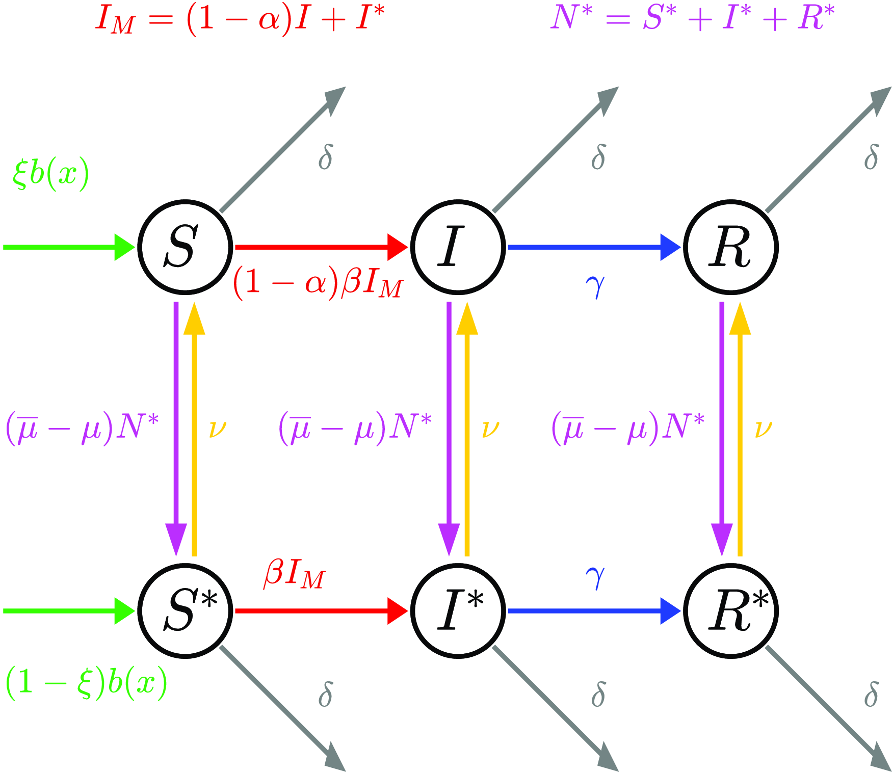


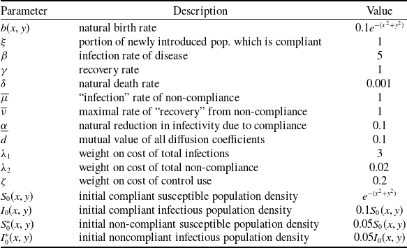


 Open access