





1. Introduction
The Navier–Stokes equations are a complex set of nonlinear equations, and their analysis often benefits from simplification. One method of simplification is to consider the linearised Navier–Stokes (LNS) equations, where linear analysis has given insights into stability and energy growth mechanisms (Ellingsen & Palm Reference Ellingsen and Palm1975; Landahl Reference Landahl1980; Gustavsson Reference Gustavsson1991). Linear analysis has been particularly insightful, given its tractability, leading to studies on transient growth (Reddy & Henningson Reference Reddy and Henningson1993) and energy amplification (Bamieh & Dahleh Reference Bamieh and Dahleh2001). This amplification arises because the LNS operator is highly non-normal. Non-normal operators allow disturbances to experience substantial transient growth even when the eigenvalues indicate asymptotic stability (Trefethen et al. Reference Trefethen, Trefethen, Reddy and Driscoll1993). Recent numerical experiments highlight the importance of transient growth mechanisms, showing that they can sustain realistic turbulence even when other linear mechanisms are suppressed (Lozano-Durán et al. Reference Lozano-Durán, Constantinou, Nikolaidis and Karp2021). Consequently, transient growth analysis is a useful tool for studying the linear amplification of disturbances in shear flows. More recently, linear analysis has proven useful even in fully turbulent flows, revealing organisation and scaling behaviours on turbulent mean flow profiles (del Álamo & Jiménez Reference del Álamo and Jiménez2006; Pujals et al. Reference Pujals, García-Villalba, Cossu and Depardon2009; Hwang & Cossu Reference Hwang and Cossu2010a ; McKeon & Sharma Reference McKeon and Sharma2010). This makes a compelling argument that linear analysis is useful in describing the dynamics of turbulence.
Linear analysis characterises the amplification of disturbances in a fluid flow (Baggett, Driscoll & Trefethen Reference Baggett, Driscoll and Trefethen1995; Brandt Reference Brandt2014). Two approaches to examine this amplification, and therefore, turbulent mechanisms, are transient growth analysis and input–output analysis. A wall-normal velocity disturbance will induce energy growth prior to decay (Gustavsson Reference Gustavsson1991). The maximum transient growth scales like $\textit {O}(R^2)$
, where
$\textit {O}(R^2)$
, where $R$
is the Reynolds number (Trefethen et al. Reference Trefethen, Trefethen, Reddy and Driscoll1993). Transient growth is greatest for initial conditions corresponding to streamwise vortices. Input–output analysis has mathematical similarities to prior work on transient growth (Butler & Farrell Reference Butler and Farrell1992), stability analysis (Drazin & Reid Reference Drazin and Reid2004) and amplification of stochastic excitations (Farrell & Ioannou Reference Farrell and Ioannou1993). Consistent with transient growth studies, input–output analyses employing stochastic (Jovanović & Bamieh Reference Jovanović and Bamieh2005) and harmonic (Schmid Reference Schmid2007) forcing demonstrate that the most amplified flow structures correspond to streamwise vortices and streaks. The resulting flow field contains streamwise-elongated large-scale flow structures (streamwise streaks).
$R$
is the Reynolds number (Trefethen et al. Reference Trefethen, Trefethen, Reddy and Driscoll1993). Transient growth is greatest for initial conditions corresponding to streamwise vortices. Input–output analysis has mathematical similarities to prior work on transient growth (Butler & Farrell Reference Butler and Farrell1992), stability analysis (Drazin & Reid Reference Drazin and Reid2004) and amplification of stochastic excitations (Farrell & Ioannou Reference Farrell and Ioannou1993). Consistent with transient growth studies, input–output analyses employing stochastic (Jovanović & Bamieh Reference Jovanović and Bamieh2005) and harmonic (Schmid Reference Schmid2007) forcing demonstrate that the most amplified flow structures correspond to streamwise vortices and streaks. The resulting flow field contains streamwise-elongated large-scale flow structures (streamwise streaks).
Streamwise streaks are organised tubes of slow- and fast-moving fluid that are susceptible to instability and breakdown (Hamilton, Kim & Waleffe Reference Hamilton, Kim and Waleffe1995; Waleffe Reference Waleffe1997). Linear analyses reveal that streaks are highly amplified (Hwang & Cossu Reference Hwang and Cossu2010a ). Streamwise streaks are also a prominent feature in fully turbulent flows in both simulations (Lee Reference Lee1991; Tsukahara, Kawamura & Shingai Reference Tsukahara, Kawamura and Shingai2006; Chau & Bhaganagar Reference Chau and Bhaganagar2012) and in experiments (Hutchins & Marusic Reference Hutchins and Marusic2007; Monty et al. Reference Monty, Stewart, Williams and Chong2007). The mechanism that drives this amplification and the formation of streamwise streaks is known as the lift-up mechanism (Ellingsen & Palm Reference Ellingsen and Palm1975; Landahl Reference Landahl1990). The lift-up process is described as the movement of low-velocity fluid from the wall upwards and vice versa (Jiménez Reference Jiménez2018). While streamwise streaks have a dominant presence in shear flows, they are not the only amplified feature that play a role in turbulence in the linear context. Tollmien–Schlichting (TS) waves (Tollmien Reference Tollmien1929; Schlichting Reference Schlichting1933; Schubauer & Skramstad Reference Schubauer and Skramstad1947; Cossu & Brandt Reference Cossu and Brandt2004) are spanwise-constant structures that play a role in turbulent transition (Sandham & Kleiser Reference Sandham and Kleiser1992). Originally, linear analysis pointed to these waves as a primary cause of transition in plane Poiseuille flow due to their instability above a critical Reynolds number (Orszag Reference Orszag1971). The critical layer mechanism plays a role in the amplification of these waves (Maslowe Reference Maslowe1986). Experiments found that transition occurs prior to this critical point; consequently, other explanations like oblique transition were considered. Oblique waves are structures angled to the streamwise direction of the flow and also contribute to turbulent transition (Duguet & Schlatter Reference Duguet and Schlatter2013; Paranjape, Duguet & Hof Reference Paranjape, Duguet and Hof2020). In a direct numerical simulation (DNS), initial conditions corresponding to an oblique pair induced rapid transition (Schmid & Henningson Reference Schmid and Henningson1992), where the linear growth mechanisms were dominant. The roles of streaks, oblique waves and TS waves in subcritical transition have been explained as input–output resonances of the spatio-temporal frequency responses (Jovanović & Bamieh Reference Jovanović and Bamieh2005).
Jovanović & Bamieh (Reference Jovanović and Bamieh2005) established that the LNS equations respond most strongly to forcing in the spanwise and wall-normal directions; the amplification is concentrated in the streamwise component and yields streamwise streaks. Using a streamwise-constant assumption, the Reynolds number scaling for amplification for both spanwise and wall-normal forcing of the streamwise velocity is shown to be $\textit {O}(R^3)$
(as opposed to
$\textit {O}(R^3)$
(as opposed to $\textit {O}(R)$
for streamwise forcing). Using a similar streamwise-constant assumption, Illingworth (Reference Illingworth2020) decomposed the LNS model into two separate subsystems, one corresponding to the Orr–Sommerfeld mechanism (Orr Reference Orr1907; Sommerfeld Reference Sommerfeld1908) and one corresponding to the Squire mechanism (Squire Reference Squire1933). This model helped explain the prevalence of streamwise streaks by showing that they are predominantly encoded within the Orr–Sommerfeld operator. These analyses, performed for streaks and set within the input–output framework, are promising tools to study TS waves and oblique waves. Such analysis would provide a more complete view of linear dynamics in the Navier–Stokes equations.
$\textit {O}(R)$
for streamwise forcing). Using a similar streamwise-constant assumption, Illingworth (Reference Illingworth2020) decomposed the LNS model into two separate subsystems, one corresponding to the Orr–Sommerfeld mechanism (Orr Reference Orr1907; Sommerfeld Reference Sommerfeld1908) and one corresponding to the Squire mechanism (Squire Reference Squire1933). This model helped explain the prevalence of streamwise streaks by showing that they are predominantly encoded within the Orr–Sommerfeld operator. These analyses, performed for streaks and set within the input–output framework, are promising tools to study TS waves and oblique waves. Such analysis would provide a more complete view of linear dynamics in the Navier–Stokes equations.
Recent work has further explored the relationship between the Orr–Sommerfeld and Squire formulation and the resolvent. Rosenberg & McKeon (Reference Rosenberg and McKeon2019) analysed exact coherent states of the Navier–Stokes equations using resolvent analysis. By examining the componentwise structure of the resolvent operator, including its Orr–Sommerfeld and Squire contributions, and applying a Helmholtz decomposition, they identified input–output relationships between forcing components and velocity responses. This approach enabled low-dimensional representations of both the forcing and response fields and further highlighted the role of the Orr–Sommerfeld and Squire operators in organising flow dynamics. While that work used the resolvent framework to analyse exact coherent states of the Navier–Stokes equations, the present study instead derives a simplified model from the LNS equations to examine amplification mechanisms associated with streaks, oblique waves and TS waves.
In the present work a simplified model is formulated from the LNS equations using an argument based on the lift-up mechanism (details given in § 2.4). Given that streamwise streaks are a prominent feature in shear flows, and these streaks are generated by the lift-up mechanism, this mechanism must be significant. We retain only the forcing pathways that contain the lift-up mechanism, a simplification that yields two key benefits. The first is that we are able to analyse the model as two separate subsystems, each containing one linear operator, or, as an Orr–Sommerfeld system in series with a Squire system. The Orr–Sommerfeld system captures the influence of the streamwise, spanwise and wall-normal forcing components on the wall-normal velocity. The Squire system captures the influence of the wall-normal velocity on the streamwise and spanwise velocity components. These two systems in series then represent how all three forcing components generate wall-normal velocity fluctuations, and in turn, how wall-normal velocity fluctuations generate the streamwise and spanwise velocity fluctuations via the wall-normal shear. The second benefit is that we can retain the spanwise wavenumber (i.e. there is no streamwise-constant assumption). As we will see, this analysis of the simplified model provides new insights into the origins and dynamics of streaks, oblique waves and TS waves. We consider three cases: laminar Couette flow, laminar Poiseuille flow and turbulent Poiseuille flow. These cases are selected to span increasing levels of dynamical complexity in canonical channel flow configurations. Laminar Couette flow represents the simplest case: it is linearly stable for all Reynolds numbers and predominantly amplifies streamwise-constant structures through non-modal mechanisms. Laminar Poiseuille flow introduces additional complexity, as it contains both strong non-modal amplification of streamwise-constant features and the TS instability. Turbulent Poiseuille flow further extends the analysis to a fully developed turbulent mean profile. Here, the linearised dynamics is evaluated about a turbulent mean profile where the nonlinear terms are treated as an intrinsic forcing. Turbulent Couette flow is not included as its dominant amplification mechanisms are dominated by streak amplification; thus, it does not introduce fundamentally new mechanisms beyond the cases already selected. Although the present study is restricted to canonical parallel flows, prior work demonstrates that locally parallel models capture the dominant amplification mechanisms in stochastically forced boundary layer flows (Ran et al. Reference Ran, Zare, Hack and Jovanović2019). Accordingly, we expect the primary mechanisms identified here to remain qualitatively relevant in spatially developing shear flows when interpreted in a local sense. These cases in conjunction with the simplified model help address two main gaps. The first concerns the influence of the spanwise wavenumber, as previous streamwise-constant models omit analysis of TS waves and oblique waves. The second concerns examination of the turbulent case, as recent studies demonstrate that linear models can capture the low-rank dynamics of turbulence (McKeon, Sharma & Jacobi Reference McKeon, Sharma and Jacobi2013; Moarref et al. Reference Moarref, Sharma, Tropp and McKeon2013; Sharma & McKeon Reference Sharma and McKeon2013; Moarref et al. Reference Moarref, Jovanović, Tropp, Sharma and McKeon2014). The link between linear operators and structures contributes to the long-term goal of understanding turbulent dynamics and benefits applications like reduced-order modelling (Moarref et al. Reference Moarref, Sharma, Tropp and McKeon2013; Illingworth, Monty & Marusic Reference Illingworth, Monty and Marusic2018) and flow control (Luhar, Sharma & McKeon Reference Luhar, Sharma and McKeon2014; Toedtli, Luhar & McKeon Reference Toedtli, Luhar and McKeon2019; Oehler & Illingworth Reference Oehler and Illingworth2021).
The current work is organised in the following sections: § 2 presents the relevant equations for the linearised model and state-space systems, discusses various norms as measures of energy and presents the simplified model; § 3 examines energy amplification and compares the LNS and simplified models; § 4 examines individual contributions of the Orr–Sommerfeld and Squire operators; § 5 compares the leading modal structures in the LNS and simplified models and outlines direct links that can be made between linear operators and dominant structures; finally, conclusions are presented in § 6.
2. Linear models and methods
2.1. The LNS equations
We consider the linearised incompressible Navier–Stokes equations,
 \begin{align} \frac {\partial \boldsymbol{u'}}{\partial t} + \boldsymbol{U} \boldsymbol{\cdot }\boldsymbol{\nabla }\boldsymbol{u'} + \boldsymbol{u'} \boldsymbol{\cdot }\boldsymbol{\nabla }\boldsymbol{U} &= -\boldsymbol{\nabla }p' + \frac {\mathrm{1}}{\mathrm{R}}\varDelta \boldsymbol{u'} + \boldsymbol{d} ,\end{align}
 \begin{align} \boldsymbol{\nabla }\boldsymbol{\cdot }\boldsymbol{u} &= 0 ,\end{align}
where $\boldsymbol {u} = [u,v,w]^T$
,
$\boldsymbol {u} = [u,v,w]^T$
, $p$
is pressure,
$p$
is pressure, $'$
denotes fluctuation about a base flow,
$'$
denotes fluctuation about a base flow, $\boldsymbol {d} = [d_x,d_y,d_z]^T$
is an external force and
$\boldsymbol {d} = [d_x,d_y,d_z]^T$
is an external force and $\varDelta := {\nabla} ^2$
is the Laplacian. The considered geometry is channel flow, where the streamwise, spanwise and wall-normal directions are denoted by
$\varDelta := {\nabla} ^2$
is the Laplacian. The considered geometry is channel flow, where the streamwise, spanwise and wall-normal directions are denoted by $x$
,
$x$
, $y$
and
$y$
and $z$
, respectively. The streamwise, spanwise and wall-normal velocities are denoted as
$z$
, respectively. The streamwise, spanwise and wall-normal velocities are denoted as $u$
,
$u$
, $v$
and
$v$
and $w$
. The inclusion of a forcing term (
$w$
. The inclusion of a forcing term ( $\boldsymbol {d}$
in (2.1)), or external excitation, is consistent with the approach for linear systems in other works (Jovanović & Bamieh Reference Jovanović and Bamieh2005; Illingworth Reference Illingworth2020). The channel walls are at
$\boldsymbol {d}$
in (2.1)), or external excitation, is consistent with the approach for linear systems in other works (Jovanović & Bamieh Reference Jovanović and Bamieh2005; Illingworth Reference Illingworth2020). The channel walls are at $z = \pm h$
and no-slip boundary conditions,
$z = \pm h$
and no-slip boundary conditions, $\boldsymbol{u}(\pm h) = 0$
and
$\boldsymbol{u}(\pm h) = 0$
and ${\partial w}/{\partial z}(\pm h) = 0$
, are applied at the two walls. The Reynolds number
${\partial w}/{\partial z}(\pm h) = 0$
, are applied at the two walls. The Reynolds number $R = u_0h/\nu$
is based on the channel half-height
$R = u_0h/\nu$
is based on the channel half-height $h$
, kinematic viscosity
$h$
, kinematic viscosity $\nu$
and characteristic velocity
$\nu$
and characteristic velocity $u_0$
. The base flow profile is denoted by
$u_0$
. The base flow profile is denoted by $\boldsymbol{U}$
, which is either a laminar profile or a time-averaged mean flow profile. For laminar flows, the base flow is unidirectional and given by
$\boldsymbol{U}$
, which is either a laminar profile or a time-averaged mean flow profile. For laminar flows, the base flow is unidirectional and given by $\boldsymbol{U} = (U(z),0,0)$
, where
$\boldsymbol{U} = (U(z),0,0)$
, where $U(z) = 1 - z^2$
for Poiseuille flow and
$U(z) = 1 - z^2$
for Poiseuille flow and $U(z) = z$
for Couette flow. In the laminar cases considered,
$U(z) = z$
for Couette flow. In the laminar cases considered, $u_0$
is the maximum velocity across the channel height and the flow is linearised about the laminar flow profile. For turbulent cases,
$u_0$
is the maximum velocity across the channel height and the flow is linearised about the laminar flow profile. For turbulent cases, $u_0$
is the friction velocity
$u_0$
is the friction velocity $u_\tau = \sqrt {\tau _w / \rho }$
, where
$u_\tau = \sqrt {\tau _w / \rho }$
, where $\tau _w$
is the wall shear stress and
$\tau _w$
is the wall shear stress and $\rho$
is density. Additional turbulent profile details are provided in § 2.3.
$\rho$
is density. Additional turbulent profile details are provided in § 2.3.
It is convenient to rewrite (2.1) and (2.2) as an input–output system containing the wall-normal velocity $w$
and the wall-normal vorticity
$w$
and the wall-normal vorticity $\eta$
(Schmid & Henningson Reference Schmid and Henningson2001). A Fourier transform in the streamwise and spanwise directions lets us rewrite the equations as
$\eta$
(Schmid & Henningson Reference Schmid and Henningson2001). A Fourier transform in the streamwise and spanwise directions lets us rewrite the equations as
 \begin{align} \frac {\partial \tilde {w}}{\partial t} &= \frac {1}{\mathcal{D}^2 - k^2}\Bigg[\Bigg[(-i k_x U)\bigl(\mathcal{D}^2 - k^2\bigr) +ik_x U^{\prime \prime } + \frac {1}{R}\bigl(\mathcal{D}^2 - k^2\bigr)^2\Bigg]\tilde {w} \nonumber\\ &\quad\vphantom {\mathcal{D}^2 - k^2} - ik_x \mathcal{D}d_x - ik_y\mathcal{D}d_y - k^2 d_z\Bigg] , \end{align}
 \begin{align} \frac {\partial \tilde {\eta }}{\partial t} &= \Bigg[- i k_x U +\frac {1}{R} \bigl(\mathcal{D}^2 - k^2\bigr)\Bigg] \tilde {\eta } +i k_y U^{\prime } \tilde {w} + ik_xd_x - ik_yd_y ,\end{align}
where $k_x$
and
$k_x$
and $k_y$
are the streamwise and spanwise wavenumbers,
$k_y$
are the streamwise and spanwise wavenumbers, $\mathcal{D} = {\partial }/{\partial z}$
,
$\mathcal{D} = {\partial }/{\partial z}$
, $k^2 = k_x^2 + k_y^2$
and a tilde denotes variables expressed in the transformed domain. The same notation is used for variables transformed in space only as well as those transformed in both space and time. These equations are put into the general state-space form,
$k^2 = k_x^2 + k_y^2$
and a tilde denotes variables expressed in the transformed domain. The same notation is used for variables transformed in space only as well as those transformed in both space and time. These equations are put into the general state-space form,
 \begin{align} \boldsymbol{x}(t) &= A\boldsymbol{x}(t) +B\boldsymbol{u}(t), \nonumber \\ \boldsymbol{y}(t) &= C\boldsymbol{x}(t), \end{align}
as
 \begin{align} \begin{bmatrix} \frac {\partial \tilde {w}}{\partial t} \\[9pt] \frac {\partial \tilde {\eta }}{\partial t} \end{bmatrix} = \underbrace {\begin{bmatrix} \varDelta ^{-1} \mathcal{L}_{\textit{OS}} & 0 \\[5pt] -ik_yU^{\prime } & \mathcal{L}_{Sq} \end{bmatrix}}_{A} \begin{bmatrix} \tilde {w} \\ \tilde {\eta } \end{bmatrix} &+ \underbrace {\begin{bmatrix} -ik_x\varDelta ^{-1}\mathcal{D} & -ik_y\varDelta ^{-1}\mathcal{D} & -k^2\varDelta ^{-1} \\[3pt] ik_y & -ik_x & 0 \end{bmatrix}}_{B} \tilde {\boldsymbol{d}}, \end{align}
 \begin{align} \begin{bmatrix} \tilde {u} \\[3pt] \tilde {v} \\[3pt] \tilde {w} \end{bmatrix} =&\underbrace {\frac {1}{k^2} \begin{bmatrix} i k_x \mathcal{D} & -i k_y \\[5pt] i k_y \mathcal{D} & i k_x \\[5pt] k^2 & 0 \end{bmatrix}}_{C} \begin{bmatrix} \tilde {w} \\ \tilde {\eta } \end{bmatrix} ,\end{align}
where
 \begin{align} \mathcal{L}_{\textit{OS}} &= -i k_x U\varDelta + ik_x U^{\prime \prime } + \frac {1}{R}\varDelta ^2 ,\end{align}
 \begin{align} \mathcal{L}_{Sq} &= -i k_x U + \frac {1}{R} \varDelta \end{align}
and $\varDelta =(\mathcal{D}^2 - k^2)$
is the Laplacian in Fourier space.
$\varDelta =(\mathcal{D}^2 - k^2)$
is the Laplacian in Fourier space.
The state-space model above is used to examine the response of the velocity fluctuations to external forcing. This model, hereon referred to as the full LNS system, has been evaluated in prior studies under stochastic (Jovanović & Bamieh Reference Jovanović and Bamieh2005) and harmonic (Schmid Reference Schmid2007; Hwang & Cossu Reference Hwang and Cossu2010a
) forcing conditions. When evaluated under harmonic forcing conditions, the frequency response of the velocity field due to the forcing vector can be measured. In order to do so, we Laplace transform the state-space system (2.6)–(2.7) and set the Laplace variable $s = i\omega$
. The result is the resolvent operator,
$s = i\omega$
. The result is the resolvent operator, $H$
, which takes the form of
$H$
, which takes the form of
 \begin{align} H \left ( k_x,k_y,\omega ,R \right ) = C \left ( k_x,k_y \right ) \left ( i\omega I - A \left ( k_x,k_y,R \right ) \right ) ^{-1}B \left ( k_x,k_y \right ) ,\end{align}
where the matrices $A$
,
$A$
, $B$
and
$B$
and $C$
are defined by our state-space system (2.6)–(2.7). For the full LNS system, the resolvent is written as
$C$
are defined by our state-space system (2.6)–(2.7). For the full LNS system, the resolvent is written as
 \begin{align} H_{\textit{LNS}}(k_x,k_y,\omega ,R) &= \frac {1}{k^2} \begin{bmatrix} ik_x\mathcal D & -ik_y \\[5pt] ik_y\mathcal D & ik_x \\[5pt] k^2 & 0 \end{bmatrix} \left ( i\omega I - \begin{bmatrix} \varDelta ^{-1}\mathcal L_{\textit{OS}} & 0 \\[5pt] -ik_yU' & \mathcal L_{Sq} \end{bmatrix} \right )^{-1}\nonumber\\&\quad\times \begin{bmatrix} -ik_x\varDelta ^{-1}\mathcal D & -ik_y\varDelta ^{-1}\mathcal D & -k^2\varDelta ^{-1} \\[5pt] ik_y & -ik_x & 0 \end{bmatrix} \!.\end{align}
Here we note several items: (i) $H ( k_x,k_y,\omega ,R )$
is a four-dimensional operator-valued function in the wall-normal direction; (ii) the input to the state-space system is the external forcing field and the output is the velocity field; (iii) the state-space model can be modified to examine the effects of individual forcing components on individual velocity components by altering the
$H ( k_x,k_y,\omega ,R )$
is a four-dimensional operator-valued function in the wall-normal direction; (ii) the input to the state-space system is the external forcing field and the output is the velocity field; (iii) the state-space model can be modified to examine the effects of individual forcing components on individual velocity components by altering the $B$
or
$B$
or $C$
matrices; (iv) while
$C$
matrices; (iv) while $H$
is dependent on
$H$
is dependent on $k_x$
,
$k_x$
, $k_y$
,
$k_y$
, $\omega$
and
$\omega$
and $R$
, this study is primarily concerned with the effect of
$R$
, this study is primarily concerned with the effect of $k_x$
and
$k_x$
and $k_y$
at a given Reynolds number and ‘worst-case’ frequency. Here, ‘worst-case’ frequency refers to the frequency producing the maximum amplification. Before the simplified model is derived (§ 2.4), we first consider options for evaluation of our three-variable (
$k_y$
at a given Reynolds number and ‘worst-case’ frequency. Here, ‘worst-case’ frequency refers to the frequency producing the maximum amplification. Before the simplified model is derived (§ 2.4), we first consider options for evaluation of our three-variable ( $k_x,k_y,\omega$
) resolvent operator at a fixed Reynolds number.
$k_x,k_y,\omega$
) resolvent operator at a fixed Reynolds number.
2.2. Transfer function norms
The energy in the velocity fields can be quantified by defining a suitable norm for the resolvent operator. The norm provides a mathematical measure of the energy contained in the velocity field, integrated over the wall-normal direction. This reduces the dimensions of our problem, allowing for analysis of the resolvent as a function of streamwise wavenumber, spanwise wavenumber and frequency. The treatment of the frequency changes with the choice of norm. The two norm (Farrell & Ioannou Reference Farrell and Ioannou1993; Bamieh & Dahleh Reference Bamieh and Dahleh2001; Jovanović & Bamieh Reference Jovanović and Bamieh2005; Hwang & Cossu Reference Hwang and Cossu2010a
), which is an average over all frequencies, and the infinity norm (Zhou, Doyle & Glover Reference Zhou, Doyle and Glover1996; Schmid Reference Schmid2007; Illingworth Reference Illingworth2020), which examines only the ‘worst-case’ frequency, are commonly used to measure the energy amplification of the resolvent operator, $H$
, in shear flows.
$H$
, in shear flows.
The infinity norm is defined as
 \begin{align} \Vert H \Vert _\infty = \underset {\omega }{\text{max}} \; \sigma _1 \left ( i \omega \right ), \end{align}
where $\sigma _1$
is the maximum singular value of
$\sigma _1$
is the maximum singular value of $H(i \omega )$
at a given
$H(i \omega )$
at a given $\omega$
. The infinity norm measures the maximum gain over all frequencies and forcing directions; this represents the ‘worst-case’ response to deterministic inputs. The infinity norm is particularly useful in this study due to its sub-multiplicative property;
$\omega$
. The infinity norm measures the maximum gain over all frequencies and forcing directions; this represents the ‘worst-case’ response to deterministic inputs. The infinity norm is particularly useful in this study due to its sub-multiplicative property;
 \begin{align} \Vert AB\Vert _{\infty }\leqslant \Vert A \Vert _{\infty }\boldsymbol{\cdot }\Vert B \Vert _{\infty }. \end{align}
The sub-multiplicative property provides a way to compare the combined amplification of systems, e.g. Orr–Sommerfeld and Squire systems, to their maximum potential amplification; where the maximum amplification is found by multiplying the optimal responses of each individual component.
On the other hand, the two norm represents an average gain over all forcing frequencies and directions. The two norm is defined as
 \begin{align} \Vert H \Vert _{2}^2 = \frac {1}{2\pi }\int _{{-\infty }}^{{\infty }} {\text{Trace}[H^*(i\omega )H(i\omega )]} \: {\rm d}{\omega }. \end{align}
The two norm is used in studies that examine stochastic forcing to determine the ensemble-average energy density of the statistically steady state (Farrell & Ioannou Reference Farrell and Ioannou1993). The two norm integrates contributions from all frequencies, helping reveal features present across a broad range of frequencies within the velocity response. The two norm can also be obtained without integration over $\omega$
by solving the Lyapunov equations
$\omega$
by solving the Lyapunov equations
 \begin{align} A\big(k_x,k_y\big) X\big(k_x,k_y\big) + X\big(k_x,k_y\big) A^*\big(k_x,k_y\big) = -B\big(k_x,k_y\big) B^*\big(k_x,k_y\big) ,\end{align}
 \begin{align} A^*\big(k_x,k_y\big) Y\big(k_x,k_y\big) + Y\big(k_x,k_y\big) A\big(k_x,k_y\big) = -C^*\big(k_x,k_y\big) C\big(k_x,k_y\big) ,\end{align}
where a $(\boldsymbol{\cdot })^*$
denotes the adjoint of the operator, and
$(\boldsymbol{\cdot })^*$
denotes the adjoint of the operator, and $X$
and
$X$
and $Y$
are referred to as the controllability and observability Gramians, respectively. The two norm is then calculated by solving the following equation:
$Y$
are referred to as the controllability and observability Gramians, respectively. The two norm is then calculated by solving the following equation:
 \begin{align} \Vert H \Vert _{2}^2 = \text{trace}\big(C\big(k_x,k_y\big)X\big(k_x,k_y\big)C^*\big(k_x,k_y\big)\big) .\end{align}
When considering amplification of the resolvent operator, the wavenumber pairs at which the maximum energy is observed are insensitive to the choice of norm. In § 3 we choose to use the infinity norm due to its sub-multiplicative property (2.13). This property allows for examination of the individual Orr–Sommerfeld and Squire systems, as well as the full LNS system (models derived in § 2.4). We will see that this analysis helps visualise how the amplification in the full system arises from the combined effects of the individual Orr–Sommerfeld and Squire components. In § 5 we examine the leading modal structures by using an eigenvalue decomposition. Unlike amplification, where different norms may yield different numerical values of the gain but typically preserve the qualitative trends, the structures obtained are more sensitive to the choice of norm. If the infinity norm is used, it can provide a limited view when evaluating leading modal structures as only one frequency is considered. For this reason, a two-norm-like approach is used to consider all frequencies by taking the eigenvalue decomposition of the response covariance matrix ( $CXC^*$
). In summary, the infinity norm is used for evaluation of amplifications to make use of the sub-multiplicative property; for modal analysis of structures, all frequencies are considered in the analysis.
$CXC^*$
). In summary, the infinity norm is used for evaluation of amplifications to make use of the sub-multiplicative property; for modal analysis of structures, all frequencies are considered in the analysis.
2.3. Turbulent Poiseuille flow details
The turbulent Poiseuille flow case requires introduction of a mean turbulent profile via an eddy-viscosity model into our state-space system. In order to evaluate our linear model about a turbulent mean profile, we introduce a Cess (Cess Reference Cess1958) eddy-viscosity model (Reynolds & Hussain Reference Reynolds and Hussain1972). The same base equation (2.1) is used with two main differences. The first is a change in the definition of the forcing terms to be equal to the remaining nonlinear terms, so that $\boldsymbol{d} = -(\boldsymbol{u} \boldsymbol{\cdot }\boldsymbol{\nabla }) \boldsymbol{u} + (\overline {\boldsymbol{u} \boldsymbol{\cdot }\boldsymbol{\nabla })\boldsymbol{u}}$
. From this viewpoint, we are now evaluating the linear response to an unknown nonlinear forcing. The second change is that we replace the laminar base flow with the time-averaged mean flow profile
$\boldsymbol{d} = -(\boldsymbol{u} \boldsymbol{\cdot }\boldsymbol{\nabla }) \boldsymbol{u} + (\overline {\boldsymbol{u} \boldsymbol{\cdot }\boldsymbol{\nabla })\boldsymbol{u}}$
. From this viewpoint, we are now evaluating the linear response to an unknown nonlinear forcing. The second change is that we replace the laminar base flow with the time-averaged mean flow profile $\boldsymbol{U}$
. The nonlinear effects are realised in both the forcing term and in setting the mean profile. The mean velocity profile is
$\boldsymbol{U}$
. The nonlinear effects are realised in both the forcing term and in setting the mean profile. The mean velocity profile is $\boldsymbol{U} = (U(z),0,0)$
, where
$\boldsymbol{U} = (U(z),0,0)$
, where $U(z)$
is obtained by integrating
$U(z)$
is obtained by integrating $R_{\tau }(1-z)\nu / \nu _{\tau }(z)$
. The eddy viscosity is defined as
$R_{\tau }(1-z)\nu / \nu _{\tau }(z)$
. The eddy viscosity is defined as
 \begin{align} \nu _{\tau }(z) = \frac {\nu }{2}\left ( 1+\frac {\kappa R^2_{\tau }}{9}\big(2z - z^2\big)^2\big(3-4z+z^2\big) \left [ 1 - \exp \left ( \frac {-R_{\tau }}{A} \right ) \right ]^2 \right )^{\tfrac {1}{2}} + \frac {\nu }{2}. \end{align}
Here $\kappa = 0.426$
and
$\kappa = 0.426$
and $A = 25.4$
(del Álamo & Jiménez Reference del Álamo and Jiménez2006; Pujals et al. Reference Pujals, García-Villalba, Cossu and Depardon2009; Hwang & Cossu Reference Hwang and Cossu2010b
) where these values are optimised for
$A = 25.4$
(del Álamo & Jiménez Reference del Álamo and Jiménez2006; Pujals et al. Reference Pujals, García-Villalba, Cossu and Depardon2009; Hwang & Cossu Reference Hwang and Cossu2010b
) where these values are optimised for $R_{\tau }=2003$
. This approximation has proven to be effective at other Reynolds numbers (Symon et al. Reference Symon, Madhusudanan, Illingworth and Marusic2023). By including the eddy viscosity, the equations for the Orr–Sommerfeld and Squire operators become
$R_{\tau }=2003$
. This approximation has proven to be effective at other Reynolds numbers (Symon et al. Reference Symon, Madhusudanan, Illingworth and Marusic2023). By including the eddy viscosity, the equations for the Orr–Sommerfeld and Squire operators become
 \begin{align} \mathcal{L}_{\textit{OS}} &= -i k_x U\varDelta + ik_x U^{\prime \prime } + \nu _{\tau }\varDelta ^2 + 2 \nu _{\tau }^{\prime } \mathcal{D} \varDelta + \nu _{\tau }^{\prime \prime } \big(\mathcal{D}^2 + k^2\big), \end{align}
 \begin{align} \mathcal{L}_{Sq} &= -i k_x U + \nu _{\tau }\varDelta + 2 \nu _{\tau }^{\prime }\mathcal{D} .\end{align}
The introduction of the eddy viscosity changes the meaning of the forcing term, $\boldsymbol{d}$
, to be an unknown nonlinear forcing as opposed to an external forcing. This change has no effect on the lift-up mechanism in the simplified model.
$\boldsymbol{d}$
, to be an unknown nonlinear forcing as opposed to an external forcing. This change has no effect on the lift-up mechanism in the simplified model.
2.4. A hypothesis for simplifying the linear system via a lift-up mechanism argument
In order to form our hypothesis and simplified model, we first present several methods of amplification in the LNS equations. Two methods of energy amplification in the resolvent are due to the non-normal amplification associated with the coupling term (i.e. the lift-up mechanism Ellingsen & Palm Reference Ellingsen and Palm1975; Landahl Reference Landahl1990; Jiménez Reference Jiménez2018) and the critical layer mechanism (McKeon et al. Reference McKeon, Sharma and Jacobi2013). A third mechanism is another non-normal amplification mechanism, the Orr mechanism (Orr Reference Orr1907). The lift-up mechanism is driven by the wall-normal shear and results in the generation of streamwise streaks (Brandt Reference Brandt2014). This mechanism can amplify an initial disturbance, where energy amplification in the time domain scales with the square of the Reynolds number (Reddy & Henningson Reference Reddy and Henningson1993). The critical layer mechanism leads to resonant interactions even when the mean shear is small (e.g. ${\rm d}U/{\rm d}z \approx 0$
), and becomes increasingly dominant at high Reynolds numbers (McKeon & Sharma Reference McKeon and Sharma2010). This mechanism is present at non-streamwise-constant wavenumbers when the local velocity is equal to the local wave speed (
${\rm d}U/{\rm d}z \approx 0$
), and becomes increasingly dominant at high Reynolds numbers (McKeon & Sharma Reference McKeon and Sharma2010). This mechanism is present at non-streamwise-constant wavenumbers when the local velocity is equal to the local wave speed ( $u(z) = \omega / k_x$
). The Orr mechanism amplifies upstream-tilted wall-normal velocity structures; this amplification occurs as the shear tilts the structures from an upstream-tilted orientation towards a vertical orientation (Jiménez Reference Jiménez2018). While the Orr mechanism can be identified directly from the linearised equations, Orr-like transient growth events have also been observed in fully turbulent flows and linked to momentum transfer and energy amplification (Encinar & Jiménez Reference Encinar and Jiménez2020; Lozano-Durán et al. Reference Lozano-Durán, Constantinou, Nikolaidis and Karp2021). The net effect of amplifying wall-normal velocity through this mechanism is the creation of streaks by the lift-up mechanism.
$u(z) = \omega / k_x$
). The Orr mechanism amplifies upstream-tilted wall-normal velocity structures; this amplification occurs as the shear tilts the structures from an upstream-tilted orientation towards a vertical orientation (Jiménez Reference Jiménez2018). While the Orr mechanism can be identified directly from the linearised equations, Orr-like transient growth events have also been observed in fully turbulent flows and linked to momentum transfer and energy amplification (Encinar & Jiménez Reference Encinar and Jiménez2020; Lozano-Durán et al. Reference Lozano-Durán, Constantinou, Nikolaidis and Karp2021). The net effect of amplifying wall-normal velocity through this mechanism is the creation of streaks by the lift-up mechanism.
We now use an argument based on the lift-up mechanism to simplify the governing equations (2.6)–(2.7). While there are multiple ways to amplify a disturbance through linear mechanisms, the presence of the lift-up mechanism stands out; it naturally follows amplification from the Orr mechanism and we observe the streamwise streaks created by it in turbulent flows. If the lift-up mechanism is important for amplification in the linearised equations then a simplified model that retains this mechanism is an interesting way to explore the underlying dynamics. The purpose of the simplified model is that amplification mechanisms can be viewed in individual linear operators. In other words, we can examine how the Orr–Sommerfeld operator (or Squire operator) amplifies streaks, oblique waves and TS waves.
The pathways in which the lift-up mechanism, the critical layer mechanism and the Orr mechanism act can be visualised by representing the LNS equations in a block diagram. The block diagram for the LNS system is depicted in figure 1(a), where we can trace individual pathways from the three forcing components to the three velocity components.
(a) Block diagram of the full LNS system, where individual forcing terms are related to individual velocity terms. (b) Block diagram of the simplified model, where individual transfer functions are linked in series, and pathways that do not contain the lift-up mechanism have been removed. (a) Full LNS model. (b) Simplified model.

Figure 1. Long description
The image contains two block diagrams. The first diagram, labeled (a), represents the full LNS system. It shows how individual forcing terms are related to individual velocity terms. The diagram includes various components such as 0, −ikx, iky, dx, dy, dz, k2, Δ, HOS(iω), −ikyU’, Hsq(iω), I, and several summation points. The second diagram, labeled (b), represents a simplified model of the LNS system. It shows individual transfer functions linked in series, with pathways that do not contain the lift-up mechanism removed. This diagram includes components such as dx, dy, dz, −ikxΔ−1D, −ikyΔ−1D, −k2Δ−1, HOS(iω), −ikyU’, Hsq(iω), −iky/k2, ikx/k2, and 0. The diagrams illustrate the relationships and flow between these components in the context of the LNS system.
The critical layer mechanism and Orr mechanism are both encoded in the Orr–Sommerfeld equation; the critical layer arising as a resolution to a singularity in the Orr–Sommerfeld equation at a critical point where the perturbation and wave speeds are equal (Maslowe Reference Maslowe1986), and the Orr mechanism in the Laplacian acting on wall-normal velocity (Jiménez Reference Jiménez2018). The lift-up mechanism requires the interaction of the Orr–Sommerfeld and Squire operators via the wall-normal shear term. The only pathway that contains the lift-up mechanism is the solid pathway in the centre of figure 1(a). We simplify the model by retaining only the centre pathway that contains the lift-up mechanism. The simplified model is shown in figure 1(b).
The model depicted in figure 1(b) is hereon referred to as the simplified model. While the simplified model is useful in enabling analysis of individual operators, we must also address two shortcomings. The first is that the simplified model only outputs streamwise and spanwise velocity components, and therefore, the model will have a lower kinetic energy under conditions where wall-normal velocity is significant. The second is that the Orr–Sommerfeld operator becomes unstable after a critical Reynolds number. For these reasons, we need to identify conditions where wall-normal velocity is not significant (as a function of $k_x$
and
$k_x$
and $k_y$
) and give consideration to stable and unstable Reynolds number regimes.
$k_y$
) and give consideration to stable and unstable Reynolds number regimes.
2.4.1. Deriving the simplified model
A natural consequence of the simplified model, as shown in figure 1(b), is that energy is contained only in the $\tilde {u}$
and
$\tilde {u}$
and $\tilde {v}$
components. This allows for scalar relationships between velocity and vorticity to be derived in Fourier space. We first consider an equation for the wall-normal vorticity as forced by the wall-normal velocity, i.e.
$\tilde {v}$
components. This allows for scalar relationships between velocity and vorticity to be derived in Fourier space. We first consider an equation for the wall-normal vorticity as forced by the wall-normal velocity, i.e.
 \begin{align} \tilde {\eta } = \left (i\omega I - \mathcal{L}_{Sq} \right )^{-1} \left (-ik_yU'\right ) \left ( i\omega I - \varDelta ^{-1} \mathcal{L}_{\textit{OS}} \right )^{-1} B_w \tilde {\boldsymbol{d}} ,\end{align}
where $B_w = \begin{bmatrix}-ik_x\varDelta ^{-1}\mathcal{D} & -ik_y\varDelta ^{-1}\mathcal{D} & -k^2\varDelta ^{-1} \end{bmatrix}$
.
$B_w = \begin{bmatrix}-ik_x\varDelta ^{-1}\mathcal{D} & -ik_y\varDelta ^{-1}\mathcal{D} & -k^2\varDelta ^{-1} \end{bmatrix}$
.
The streamwise and spanwise velocity can then be expressed as
 \begin{align} \tilde {u} &= \frac {-ik_y}{k^2} \tilde {\eta },\\[-12pt]\nonumber \end{align}
 \begin{align} \tilde {v} &= \frac {ik_x}{k^2} \tilde {\eta }.\end{align}
These relationships hold if the contribution of the wall-normal velocity as an output can be neglected. In other words, if the flow field is primarily composed of a streamwise and spanwise velocity response (for a given $k_x$
,
$k_x$
, $k_y$
), we can ignore the small wall-normal velocity contribution to the flow field. To identify the parameter space in which the model will perform the best, the infinity norm for the wall-normal velocity component,
$k_y$
), we can ignore the small wall-normal velocity contribution to the flow field. To identify the parameter space in which the model will perform the best, the infinity norm for the wall-normal velocity component, $\Vert H_{w}\Vert _\infty$
, is compared with the infinity norm for all three velocity components,
$\Vert H_{w}\Vert _\infty$
, is compared with the infinity norm for all three velocity components, $\Vert H \Vert _\infty$
, in figure 2 for laminar Poiseuille flow.
$\Vert H \Vert _\infty$
, in figure 2 for laminar Poiseuille flow.
Plot of ${\Vert H_{w}\Vert _\infty }/{\Vert H \Vert _\infty }$
using the infinity norm at
${\Vert H_{w}\Vert _\infty }/{\Vert H \Vert _\infty }$
using the infinity norm at $R$
= 2000 for Poiseuille flow. Oval region (labelled I) depicts a wavenumber space around
$R$
= 2000 for Poiseuille flow. Oval region (labelled I) depicts a wavenumber space around $k_x \sim O(1)$
that can contain TS-wave amplification in Poiseuille flow.
$k_x \sim O(1)$
that can contain TS-wave amplification in Poiseuille flow.

Figure 2. Long description
A heat map with logarithmic axes labeled kx and ky represents wavenumber space for Poiseuille flow analysis. The color scale ranges from light blue to dark blue, indicating varying levels of intensity. An oval region labeled I highlights a specific area of interest where TS-wave amplification can occur. The heat map shows a gradient of intensity, with darker colors representing higher values and lighter colors representing lower values. The axes range from 10^−4 to 10^2 for both kx and ky, capturing a wide spectrum of wavenumbers. The heat map is used to analyze the linear amplification of disturbances in Poiseuille flow, particularly focusing on transient growth mechanisms.
In figure 2, for wavenumber pairs in the region bounded by $1\times 10^{-4} \lt k_x \lt 1$
and
$1\times 10^{-4} \lt k_x \lt 1$
and $0.01 \lt k_y \lt 50$
, we see that the wall-normal velocity component contributes
$0.01 \lt k_y \lt 50$
, we see that the wall-normal velocity component contributes $\lt$
30 % of the total energy. The majority of wavenumber pairs in this same region have a wall-normal velocity contribution below 1 % (white). Therefore, in the considered wavenumber space (§ 2.5), the contribution of the wall-normal velocity to the total energy is negligible when compared with the streamwise and spanwise contribution. There is one exception for the horizontal band around
$\lt$
30 % of the total energy. The majority of wavenumber pairs in this same region have a wall-normal velocity contribution below 1 % (white). Therefore, in the considered wavenumber space (§ 2.5), the contribution of the wall-normal velocity to the total energy is negligible when compared with the streamwise and spanwise contribution. There is one exception for the horizontal band around $k_x \sim O(1)$
, a region containing TS waves (see region labelled I in figure 2). Here, the assumption of negligible wall-normal velocity is no longer valid and model discrepancies are expected. These discrepancies are highlighted in § 3 and characterised further in § 3.2.
$k_x \sim O(1)$
, a region containing TS waves (see region labelled I in figure 2). Here, the assumption of negligible wall-normal velocity is no longer valid and model discrepancies are expected. These discrepancies are highlighted in § 3 and characterised further in § 3.2.
The equations for the simplified model contain the individual contributions of the Orr–Sommerfeld operator and separately the Squire operator. When placed in series, they produce a system that is equivalent to figure 1(b). Here, the wall-normal velocity serves as the input to the Squire system, and the wall-normal vorticity is the only input to the velocity components. Now that the model is simplified, it is translated back into a state-space system for calculations. The modified equations are shown below in state-space format, i.e.
 \begin{align} \frac {\partial \tilde {w}}{\partial t} = \varDelta ^{-1} \mathcal{L}_{\textit{OS}} \tilde {w} &+ \begin{bmatrix} -ik_x\varDelta ^{-1}\mathcal{D} & -ik_y\varDelta ^{-1}\mathcal{D} & -k^2\varDelta ^{-1} \end{bmatrix} \tilde {\boldsymbol{d}}, \\[-12pt]\nonumber \end{align}
 \begin{align} &\quad \quad \tilde {w} = I \tilde {w}, \\[-12pt]\nonumber \end{align}
 \begin{align} &\frac {\partial \tilde {\eta }}{\partial t} = \mathcal{L}_{Sq} \tilde {\eta } + -ik_yU^{\prime } \tilde {w}, \\[-12pt]\nonumber \end{align}
 \begin{align} &\, \begin{bmatrix} \tilde {u} \\ \tilde {v} \end{bmatrix} = \frac {1}{k^2} \begin{bmatrix} -i k_y \\ i k_x \end{bmatrix} \lbrack \tilde {\eta } \rbrack ,\end{align}
so that the overall system can be written as
 \begin{align} \begin{bmatrix} \frac {\partial \tilde {w}}{\partial t} \\[9pt] \frac {\partial \tilde {\eta }}{\partial t} \end{bmatrix} = \begin{bmatrix} \varDelta ^{-1} \mathcal{L}_{\textit{OS}} & 0 \\[5pt] -ik_yU^{\prime } & \mathcal{L}_{Sq} \end{bmatrix} \begin{bmatrix} \tilde {w} \\ \tilde {\eta } \end{bmatrix} &+ \begin{bmatrix} -ik_x\varDelta ^{-1}\mathcal{D} & -ik_y\varDelta ^{-1}\mathcal{D} & -k^2\varDelta ^{-1} \\[5pt] 0 & 0 & 0 \end{bmatrix} \tilde {\boldsymbol{d}},\\[-12pt]\nonumber \end{align}
 \begin{align} \begin{bmatrix} \tilde {u} \\[3pt] \tilde {v} \end{bmatrix} &= \frac {1}{k^2} \begin{bmatrix} 0 & -i k_y \\[5pt] 0 & i k_x \\ \end{bmatrix} \begin{bmatrix} \tilde {w} \\[3pt] \tilde {\eta } \end{bmatrix}.\end{align}
Equations (2.24)–(2.25) represent a simplified Orr–Sommerfeld system, (2.26)–(2.27) represent a simplified Squire system and (2.28)–(2.29) represent the simplified model where the two subsystems are connected in series. Equations (2.24)–(2.29) are the mathematical equivalent of the block diagram in figure 1(b).
Forming the simplified model allows us to individually express the linear operators using the resolvent. The resolvent forms of the operators are
 \begin{align} H_{\textit{OS}}(k_x,k_y,\omega ,R) = \left ( i\omega I - \varDelta ^{-1}\mathcal L_{\textit{OS}} \right )^{-1} \end{align}
and
 \begin{align} H_{Sq}(k_x,k_y,\omega ,R) = \left ( i\omega I - \mathcal L_{Sq} \right )^{-1}. \end{align}
For the simple model, the resolvent then becomes
 \begin{align} \begin{aligned} H_{\textit{simple}}(k_x,k_y,\omega ,R) &= \frac {1}{k^2} \begin{bmatrix} 0 & -ik_y \\[3pt] 0 & ik_x \end{bmatrix} \left ( i\omega I - \begin{bmatrix} \varDelta ^{-1}\mathcal L_{\textit{OS}} & 0 \\[3pt] -ik_yU' & \mathcal L_{Sq} \end{bmatrix} \right )^{-1} \\ &\quad\times \begin{bmatrix} -ik_x\varDelta ^{-1}\mathcal D & -ik_y\varDelta ^{-1}\mathcal D & -k^2\varDelta ^{-1} \\[3pt] 0 & 0 & 0 \end{bmatrix} .\end{aligned} \end{align}
These operators can then be evaluated to determine their response to input forcings. For example, the input–output response of the Orr–Sommerfeld subsystem to the forcing $\tilde {\boldsymbol d}$
is given by
$\tilde {\boldsymbol d}$
is given by
 \begin{align} \tilde {w} = H_{\textit{OS}}(k_x,k_y,\omega ,R) \begin{bmatrix} -ik_x\varDelta ^{-1}\mathcal D & -ik_y\varDelta ^{-1}\mathcal D & -k^2\varDelta ^{-1} \end{bmatrix} \tilde {\boldsymbol d}. \end{align}
Similarly, the response of the Squire subsystem to $\tilde {w}$
(including the coupling term
$\tilde {w}$
(including the coupling term $-ik_y U'$
) is evaluated as
$-ik_y U'$
) is evaluated as
 \begin{align} \tilde {\eta } = H_{Sq}(k_x,k_y,\omega ,R) \left ( -ik_y U' \right ) \tilde {w}. \end{align}
This relationship can then be used with (2.22)–(2.23) to obtain $\tilde {u}$
and
$\tilde {u}$
and $\tilde {v}$
.
$\tilde {v}$
.
2.4.2. Pathways affected by Orr–Sommerfeld
For laminar Poiseuille flow there is a scenario where the Orr–Sommerfeld operator can become unstable; this occurs when the Reynolds number exceeds the stability limit. When $R \gt 5772$
, the Orr–Sommerfeld operator becomes unstable (Orszag Reference Orszag1971) and any pathway that includes this operator can experience exponential growth. In figure 1(a) there are three pathways from the forcing inputs
$R \gt 5772$
, the Orr–Sommerfeld operator becomes unstable (Orszag Reference Orszag1971) and any pathway that includes this operator can experience exponential growth. In figure 1(a) there are three pathways from the forcing inputs $(\tilde {d}_x,\tilde {d}_y,\tilde {d}_z)$
to the velocity outputs
$(\tilde {d}_x,\tilde {d}_y,\tilde {d}_z)$
to the velocity outputs $(\tilde {u},\tilde {v},\tilde {w})$
. The simplified model includes one of these paths (solid pathway); however, the Orr–Sommerfeld operator is also included in the dash-dot pathway in figure 1(a), and is therefore of interest as well. To address this, we form an additional model that captures this pathway.
$(\tilde {u},\tilde {v},\tilde {w})$
. The simplified model includes one of these paths (solid pathway); however, the Orr–Sommerfeld operator is also included in the dash-dot pathway in figure 1(a), and is therefore of interest as well. To address this, we form an additional model that captures this pathway.
Block diagram of the Orr–Sommerfeld system, where only the dash-dot path from figure 1(a) is retained.

Figure 3. Long description
The block diagram of the OrrSommerfeld system features three input variables labeled d_tilde_x, d_tilde_y, and d_tilde_z. Each input variable is processed through a series of operations: d_tilde_x through −i k_x Δ inverse D, d_tilde_y through −i k_y Δ inverse D, and d_tilde_z through −k squared Δ inverse. The outputs of these operations are summed together and fed into a block labeled H_O S (i ω). The output of this block, labeled w_tilde, is then split into three paths. Each path processes w_tilde through different operations: i k_y D over k squared, i k_x D over k squared, and an identity operation labeled I. These operations produce the final outputs labeled u_tilde, v_tilde, and w_tilde respectively.
The block diagram in figure 3 follows the pathway from the external forcing through the Orr–Sommerfeld operator and directly to $\tilde {u}$
,
$\tilde {u}$
, $\tilde {v}$
and
$\tilde {v}$
and $\tilde {w}$
(as opposed to passing through the Squire operator). This block diagram is exactly the dash-dot pathway from figure 1(a). We refer to this model as the Orr–Sommerfeld model. While we do not examine cases where
$\tilde {w}$
(as opposed to passing through the Squire operator). This block diagram is exactly the dash-dot pathway from figure 1(a). We refer to this model as the Orr–Sommerfeld model. While we do not examine cases where $R \gt 5772$
, analysis of the Orr–Sommerfeld model can still provide insights into which structures are amplified in this subsystem. The Orr–Sommerfeld model is analysed in § 5.3, where the structural analysis provides a clear picture of the dynamics of the dash-dot pathway in terms of the leading modal shape, and gives insight into the modes that become unstable in laminar Poiseuille flow.
$R \gt 5772$
, analysis of the Orr–Sommerfeld model can still provide insights into which structures are amplified in this subsystem. The Orr–Sommerfeld model is analysed in § 5.3, where the structural analysis provides a clear picture of the dynamics of the dash-dot pathway in terms of the leading modal shape, and gives insight into the modes that become unstable in laminar Poiseuille flow.
2.5. Numerical parameters and structure details
The governing equations are discretised using Chebyshev polynomials with $N=75$
(laminar base flow) and
$N=75$
(laminar base flow) and $N=151$
(turbulent base flow) collocation points in the wall-normal direction. Convergence of the results has been checked by doubling the number of Chebyshev collocation points and ensuring that there was a negligible change in the results. In the wall-parallel plane we discretise using
$N=151$
(turbulent base flow) collocation points in the wall-normal direction. Convergence of the results has been checked by doubling the number of Chebyshev collocation points and ensuring that there was a negligible change in the results. In the wall-parallel plane we discretise using $k_{x_{{min}}}$
=
$k_{x_{{min}}}$
= $10^{-4}$
,
$10^{-4}$
, $k_{x_{{max}}}$
= 3.02,
$k_{x_{{max}}}$
= 3.02, $k_{y_{{min}}}$
=
$k_{y_{{min}}}$
= $10^{-2}$
and
$10^{-2}$
and $k_{y_{{max}}}$
= 15.84 with 50 Fourier modes in the streamwise and spanwise directions.
$k_{y_{{max}}}$
= 15.84 with 50 Fourier modes in the streamwise and spanwise directions.
In this paper we frequently reference well-known structures such as streamwise streaks, oblique waves and TS waves. While these structures are commonly referred to in the literature, there is no universal definition of the wavenumbers that correspond to these features. For example, while an oblique wave can be referred to as any structure with a non-zero streamwise and spanwise wavenumber, the oblique waves that receive the most attention are $(k_x = 1, k_y=1)$
in linear studies (Jovanović & Bamieh Reference Jovanović and Bamieh2005; Schmid Reference Schmid2007) or oblique waves between the angles of
$(k_x = 1, k_y=1)$
in linear studies (Jovanović & Bamieh Reference Jovanović and Bamieh2005; Schmid Reference Schmid2007) or oblique waves between the angles of $20^{\circ }$
and
$20^{\circ }$
and $32^{\circ }$
that play a role in laminar–turbulent bands (Prigent et al. Reference Prigent, Grégoire, Chaté and Dauchot2003; Kanazawa Reference Kanazawa2018; Liu & Gayme Reference Liu and Gayme2021). To address this, in this paper we use the definitions provided in table 1 when referring to streaks, oblique waves and TS waves. Additionally, figure 4 denotes the generalised locations of structures as a function of
$32^{\circ }$
that play a role in laminar–turbulent bands (Prigent et al. Reference Prigent, Grégoire, Chaté and Dauchot2003; Kanazawa Reference Kanazawa2018; Liu & Gayme Reference Liu and Gayme2021). To address this, in this paper we use the definitions provided in table 1 when referring to streaks, oblique waves and TS waves. Additionally, figure 4 denotes the generalised locations of structures as a function of $k_x$
and
$k_x$
and $k_y$
.
$k_y$
.
Summary of structures and their corresponding wavenumbers $k_x$
and
$k_x$
and $k_y$
.
$k_y$
.

Cartoon showing the generalised structure locations for streaks, oblique waves (shown here with $k_x \approx 1$
,
$k_x \approx 1$
, $k_y \approx \pm 1$
superimposed) and TS waves. Note that while all wavenumber pairs where
$k_y \approx \pm 1$
superimposed) and TS waves. Note that while all wavenumber pairs where $k_x$
and
$k_x$
and $k_y$
are non-zero are technically oblique, this study focuses mainly on the most amplified pair at
$k_y$
are non-zero are technically oblique, this study focuses mainly on the most amplified pair at $k_x \approx 1$
,
$k_x \approx 1$
, $k_y \approx 1$
. Three-dimensional call-outs depict physical structures observed in a DNS. Streaks and oblique waves are shown using streamwise velocity contours and TS waves are shown using wall-normal velocity contours (positive, red; negative, blue).
$k_y \approx 1$
. Three-dimensional call-outs depict physical structures observed in a DNS. Streaks and oblique waves are shown using streamwise velocity contours and TS waves are shown using wall-normal velocity contours (positive, red; negative, blue).

Figure 4. Long description
A line graph illustrates the generalised structure locations for streaks, oblique waves, and TS waves in the context of NavierStokes equations. The x-axis represents the wavenumber k_y, ranging from 10^−2 to 10^1, while the y-axis represents the wavenumber k_x, ranging from 10^−4 to 10^0. The graph highlights three key regions: TS waves approximately at (1, 0), oblique waves approximately at (1, 1), and streaks approximately at (0, 1.66). Three-dimensional call-outs depict physical structures observed in direct numerical simulations (DNS). Streaks and oblique waves are shown using streamwise velocity contours, while TS waves are shown using wall-normal velocity contours, with positive values in red and negative values in blue. All values are approximated.
The locations in figure 4 represent the highly amplified wavenumber pairs previously identified in linear studies (Jovanović & Bamieh Reference Jovanović and Bamieh2005; Schmid Reference Schmid2007). An analysis examining amplification from a single forcing component into a single velocity component identified several amplification mechanisms that are responsible for the creation of (i) streamwise streaks with peak values at $k_x \approx 0$
,
$k_x \approx 0$
, $k_y \approx 1$
; (ii) oblique waves with peak values at
$k_y \approx 1$
; (ii) oblique waves with peak values at $k_x \approx 1$
,
$k_x \approx 1$
, $k_y \approx 1$
; (iii) TS waves with peak values at
$k_y \approx 1$
; (iii) TS waves with peak values at $k_x \approx 1$
,
$k_x \approx 1$
, $k_y \approx 0$
(Jovanović & Bamieh Reference Jovanović and Bamieh2005). The observations were made by examining all nine possible combinations of input–output pairs. For example, the ‘mechanism that transforms low-amplitude streamwise vortices (
$k_y \approx 0$
(Jovanović & Bamieh Reference Jovanović and Bamieh2005). The observations were made by examining all nine possible combinations of input–output pairs. For example, the ‘mechanism that transforms low-amplitude streamwise vortices ( $v$
-
$v$
- $w$
-input) into large-energy streaks (
$w$
-input) into large-energy streaks ( $u$
-output)’ (Schmid Reference Schmid2007) is seen in plots showing the influence of spanwise or wall-normal forcing on the streamwise velocity. In these studies it is observed that there are multiple instances of oblique waves that are amplified, particularly along a ridge where
$u$
-output)’ (Schmid Reference Schmid2007) is seen in plots showing the influence of spanwise or wall-normal forcing on the streamwise velocity. In these studies it is observed that there are multiple instances of oblique waves that are amplified, particularly along a ridge where $k_x = k_y$
. Figure 4 uses the peak amplification values from all nine plots (using present data for contours) to highlight the general structure locations identified by Jovanović (Reference Jovanović and Bamieh2005). The call-outs in the figure show velocity contours that depict physical space representations of the structures.
$k_x = k_y$
. Figure 4 uses the peak amplification values from all nine plots (using present data for contours) to highlight the general structure locations identified by Jovanović (Reference Jovanović and Bamieh2005). The call-outs in the figure show velocity contours that depict physical space representations of the structures.
3. Energy amplification in the full LNS system and the simple model
We begin our analysis by showing the infinity norm of the transfer function, $H$
, (2.10) for all three shear flow profiles and both the LNS and simplified models. This is done as a function of wavenumbers (
$H$
, (2.10) for all three shear flow profiles and both the LNS and simplified models. This is done as a function of wavenumbers ( $k_x$
,
$k_x$
, $k_y$
) to highlight regions in Fourier space where the energy amplification potential is greatest. We will see that the peak amplification in wavenumber space is associated with three physical features: streamwise streaks, oblique waves and TS waves. If a particular region in wavenumber space is highly amplified, it indicates the presence of a dominant mechanism for the given shear flow profile. This analysis connects amplification in wavenumber space to physical features and mechanisms in three distinct shear flow cases. The simplified model serves to clarify these relationships, revealing precisely what forcing pathways are needed to capture individual flow features. Finally, the individual contributions of the Orr–Sommerfeld and Squire operators are examined to link linear mechanisms and linear operators.
$k_y$
) to highlight regions in Fourier space where the energy amplification potential is greatest. We will see that the peak amplification in wavenumber space is associated with three physical features: streamwise streaks, oblique waves and TS waves. If a particular region in wavenumber space is highly amplified, it indicates the presence of a dominant mechanism for the given shear flow profile. This analysis connects amplification in wavenumber space to physical features and mechanisms in three distinct shear flow cases. The simplified model serves to clarify these relationships, revealing precisely what forcing pathways are needed to capture individual flow features. Finally, the individual contributions of the Orr–Sommerfeld and Squire operators are examined to link linear mechanisms and linear operators.
3.1. Linear amplification in different shear flow profiles
Figure 5 shows energy amplification, using the infinity norm, for different shear flow profiles and both models. Plots contain the combined effects from all forcing directions, $\tilde {d}_x,\tilde {d}_y,\tilde {d}_z$
, and velocity components,
$\tilde {d}_x,\tilde {d}_y,\tilde {d}_z$
, and velocity components, $\tilde {u},\tilde {v},\tilde {w}$
. The rows contain the full LNS system (panels a,b,c) and the simplified model (panels d,e, f); columns contain different flow profiles.
$\tilde {u},\tilde {v},\tilde {w}$
. The rows contain the full LNS system (panels a,b,c) and the simplified model (panels d,e, f); columns contain different flow profiles.
Plots of $\log _{10}({\Vert H\Vert _\infty })$
for (a,d) laminar Couette flow, (b,e) laminar Poiseuille flow for
$\log _{10}({\Vert H\Vert _\infty })$
for (a,d) laminar Couette flow, (b,e) laminar Poiseuille flow for $R = 2000$
, and (c, f) turbulent Poiseuille flow at
$R = 2000$
, and (c, f) turbulent Poiseuille flow at $R_{\tau } = 2000$
using the full LNS model (a,b,c) and the simplified model (d,e, f), where all forcing input directions (
$R_{\tau } = 2000$
using the full LNS model (a,b,c) and the simplified model (d,e, f), where all forcing input directions ( $\tilde {d_x},\tilde {d_y},\tilde {d_z}$
) and all velocity components (
$\tilde {d_x},\tilde {d_y},\tilde {d_z}$
) and all velocity components ( $\tilde {u},\tilde {v},\tilde {w}$
) are considered. Oval and rectangular regions (labelled I–VI) are used to highlight disagreement between the LNS model and the simple model.
$\tilde {u},\tilde {v},\tilde {w}$
) are considered. Oval and rectangular regions (labelled I–VI) are used to highlight disagreement between the LNS model and the simple model.

Figure 5. Long description
The image contains six contour plots arranged in two rows and three columns. Each plot represents fluid flow analysis under different conditions and models. The top row shows results for laminar Couette flow, laminar Poiseuille flow, and turbulent Poiseuille flow using the full LNS model. The bottom row shows similar conditions using a simplified model. Each plot has axes labeled with kx and ky, representing wavenumbers in the streamwise and spanwise directions, respectively. The color scale indicates the magnitude of the response, with darker blues representing higher values. Oval and rectangular regions labeled I, II, III, IV, V, and VI highlight areas of disagreement between the LNS model and the simplified model.
From previous studies, it is known that streamwise streaks are a dominant feature in all the shear flow profiles we consider (Kitoh & Umeki Reference Kitoh and Umeki2008; Lee et al. Reference Lee, Lee, Choi and Sung2014). Additionally, oblique waves are observed as a path to transition in both Poiseuille and Couette flow due to three-dimensional interactions (Orszag & Kells Reference Orszag and Kells1980). On the other hand, TS waves are stable in Couette flow (Davey Reference Davey1973), making their instability of primary interest in only our Poiseuille flow cases. At a glance, these trends remain true for the full LNS model in figure 5 (streaks at $k_x \approx 0$
,
$k_x \approx 0$
, $k_y \approx 1.66$
; oblique waves at
$k_y \approx 1.66$
; oblique waves at $k_x \approx 1$
,
$k_x \approx 1$
, $k_y \approx 1$
; TS waves at
$k_y \approx 1$
; TS waves at $k_x \approx 1$
,
$k_x \approx 1$
, $k_y \approx 0$
). However, a more detailed analysis of each shear flow profile reveals differences in the full LNS and simplified models.
$k_y \approx 0$
). However, a more detailed analysis of each shear flow profile reveals differences in the full LNS and simplified models.
The infinity norm of the resolvent as a function of ( $k_x,k_y$
) for Couette flow is shown in figure 5(a,d). Couette flow contains persistent large-scale streamwise streaks, both in numerical simulations (Lee & Moser Reference Lee and Moser2018; Tao, Eckhardt & Xiong Reference Tao, Eckhardt and Xiong2018; Illingworth Reference Illingworth2020) and in experiments (Tillmark & Alfredsson Reference Tillmark and Alfredsson1998; Kitoh & Umeki Reference Kitoh and Umeki2008). The dominance of these structures increases with increasing Reynolds number, where they can contribute up to 50 % of the Reynolds shear stresses (Pirozzoli, Bernardini & Orlandi Reference Pirozzoli, Bernardini and Orlandi2014). Examining laminar Couette flow, with its single dominant mechanism, therefore presents the simplest case. Here, a successful model needs to capture amplification of streamwise streaks only. In figure 5(a,d), both the full LNS and simplified models show amplification in the streamwise streak region near
$k_x,k_y$
) for Couette flow is shown in figure 5(a,d). Couette flow contains persistent large-scale streamwise streaks, both in numerical simulations (Lee & Moser Reference Lee and Moser2018; Tao, Eckhardt & Xiong Reference Tao, Eckhardt and Xiong2018; Illingworth Reference Illingworth2020) and in experiments (Tillmark & Alfredsson Reference Tillmark and Alfredsson1998; Kitoh & Umeki Reference Kitoh and Umeki2008). The dominance of these structures increases with increasing Reynolds number, where they can contribute up to 50 % of the Reynolds shear stresses (Pirozzoli, Bernardini & Orlandi Reference Pirozzoli, Bernardini and Orlandi2014). Examining laminar Couette flow, with its single dominant mechanism, therefore presents the simplest case. Here, a successful model needs to capture amplification of streamwise streaks only. In figure 5(a,d), both the full LNS and simplified models show amplification in the streamwise streak region near $k_x \approx 0$
,
$k_x \approx 0$
, $k_y \approx 1.66$
. The good agreement between the two models indicates that the forcing required to generate streamwise streaks has been retained in the simplified set of equations. While streamwise streaks are the most persistent feature in Couette flow, other less amplified structures still exist. For example, the amplification of oblique waves around
$k_y \approx 1.66$
. The good agreement between the two models indicates that the forcing required to generate streamwise streaks has been retained in the simplified set of equations. While streamwise streaks are the most persistent feature in Couette flow, other less amplified structures still exist. For example, the amplification of oblique waves around $k_x \approx 1$
,
$k_x \approx 1$
, $k_y \approx 1$
is still present, however, these structures are not as amplified as the streaks. The agreement in this region is good when comparing the two models. Tollmien–Schlichting waves are also observed at a lower amplification (compared with streaks), where in figure 5(a) a small, light blue, horizontal region exists in the contours around
$k_y \approx 1$
is still present, however, these structures are not as amplified as the streaks. The agreement in this region is good when comparing the two models. Tollmien–Schlichting waves are also observed at a lower amplification (compared with streaks), where in figure 5(a) a small, light blue, horizontal region exists in the contours around $k_x \approx 1$
,
$k_x \approx 1$
, $k_y \approx 0$
. For the simplified model (figure 5
d) however, this same feature does not exist. Compare regions labelled I and II in figure 5(a,d).
$k_y \approx 0$
. For the simplified model (figure 5
d) however, this same feature does not exist. Compare regions labelled I and II in figure 5(a,d).
The infinity norm of the resolvent for the laminar Poiseuille flow case is shown in figure 5(b,e). In the full LNS model (figure 5
b), there are three regions where amplification occurs. The first region corresponds to streamwise streaks for which $k_x$
$k_x$ $\approx$
0,
$\approx$
0, $k_y$
$k_y$ $\approx$
1.66. The second region corresponds to TS waves for which
$\approx$
1.66. The second region corresponds to TS waves for which $k_x$
$k_x$ $\approx$
1,
$\approx$
1, $k_y$
$k_y$ $\approx$
0. The third is at the intersection of these regions,
$\approx$
0. The third is at the intersection of these regions, $k_x$
$k_x$ $\approx$
1,
$\approx$
1, $k_y$
$k_y$ $\approx$
1, where the most amplified oblique waves are present. Figure 5(e) shows the laminar Poiseuille case for the simplified model. There is excellent agreement in the region corresponding to streamwise streaks and oblique waves. However, in the region corresponding to TS waves, the model shows poor agreement. Compare regions labelled III and IV in figure 5(b,e). It is clear the simplified model contains the necessary components for streamwise streaks and oblique waves, but not TS waves.
$\approx$
1, where the most amplified oblique waves are present. Figure 5(e) shows the laminar Poiseuille case for the simplified model. There is excellent agreement in the region corresponding to streamwise streaks and oblique waves. However, in the region corresponding to TS waves, the model shows poor agreement. Compare regions labelled III and IV in figure 5(b,e). It is clear the simplified model contains the necessary components for streamwise streaks and oblique waves, but not TS waves.
The infinity norm of the resolvent for the turbulent Poiseuille flow case is shown in figure 5(c, f). Here, we use the modified Orr–Sommerfeld and Squire equations from § 2.3. In terms of streaks, oblique waves and TS waves, the results for the simplified model and full model are in good agreement. The results for the streamwise streak region in both the simplified and full model are nearly identical in both magnitude and shape. The observed differences are similar to the laminar cases. The first notable difference is that the TS-wave region ( $k_x \approx 1$
,
$k_x \approx 1$
, $k_y \approx 0$
) disappears in the simplified model. This comparison indicates that the simplified model lacks the necessary forcing components to reproduce TS waves. The second notable difference is the region around
$k_y \approx 0$
) disappears in the simplified model. This comparison indicates that the simplified model lacks the necessary forcing components to reproduce TS waves. The second notable difference is the region around $k_x \le 0.1, k_y \le 0.5$
where amplification is diminished in the simple model for the turbulent Poiseuille flow case (e.g. compare regions labelled V and VI in figure 5
c,f). In the full LNS model, the behaviour in region V arises from the inclusion of the eddy-viscosity term in the linearised equations. When the turbulent mean profile is used without an eddy viscosity, the amplification becomes qualitatively similar to that of the laminar Poiseuille case (as verified by additional computations, not shown). This demonstrates that the observed change in behaviour is primarily due to the eddy-viscosity modification of the linear dynamics, rather than the turbulent mean profile itself. We also note that the low wavenumbers (region V) do not become more amplified in the presence of an eddy viscosity; rather, the peak amplification in the streamwise streak region is reduced (e.g.
$k_x \le 0.1, k_y \le 0.5$
where amplification is diminished in the simple model for the turbulent Poiseuille flow case (e.g. compare regions labelled V and VI in figure 5
c,f). In the full LNS model, the behaviour in region V arises from the inclusion of the eddy-viscosity term in the linearised equations. When the turbulent mean profile is used without an eddy viscosity, the amplification becomes qualitatively similar to that of the laminar Poiseuille case (as verified by additional computations, not shown). This demonstrates that the observed change in behaviour is primarily due to the eddy-viscosity modification of the linear dynamics, rather than the turbulent mean profile itself. We also note that the low wavenumbers (region V) do not become more amplified in the presence of an eddy viscosity; rather, the peak amplification in the streamwise streak region is reduced (e.g. $\log _{10} (\Vert H \Vert _{\infty } ) \approx 4$
in the laminar case and
$\log _{10} (\Vert H \Vert _{\infty } ) \approx 4$
in the laminar case and $\log _{10} (\Vert H \Vert _{\infty } ) \approx 1.4$
in the turbulent case), which makes the low-wavenumber response appear relatively more prominent. The drop in amplification observed in the simplified model is instead related to the removal of the forcing terms (
$\log _{10} (\Vert H \Vert _{\infty } ) \approx 1.4$
in the turbulent case), which makes the low-wavenumber response appear relatively more prominent. The drop in amplification observed in the simplified model is instead related to the removal of the forcing terms ( $\tilde {\boldsymbol{d}}$
) acting on the Squire equation when deriving the simple model. This mechanism is discussed further in § 3.2.3.
$\tilde {\boldsymbol{d}}$
) acting on the Squire equation when deriving the simple model. This mechanism is discussed further in § 3.2.3.
3.2. Model validation
An analysis of individual input–output responses for the LNS system identified several amplification mechanisms responsible for creating streaks, oblique waves and TS waves (Jovanović & Bamieh Reference Jovanović and Bamieh2005). To address the agreements and disagreements in the model, we briefly consider the resolvent operator broken down into individual forcing components ( $\tilde {d}_x,\tilde {d}_y,\tilde {d}_z$
) and individual velocity responses (
$\tilde {d}_x,\tilde {d}_y,\tilde {d}_z$
) and individual velocity responses ( $\tilde {u},\tilde {v},\tilde {w}$
). By conducting a componentwise comparison, where single-input, single-output pairs are examined, we expand on the comparison performed in figure 5 in two ways: (i) highlight specifically which dominant mechanisms are captured by the simplified model for individual forcing and response pairs (e.g. streamwise streaks via
$\tilde {u},\tilde {v},\tilde {w}$
). By conducting a componentwise comparison, where single-input, single-output pairs are examined, we expand on the comparison performed in figure 5 in two ways: (i) highlight specifically which dominant mechanisms are captured by the simplified model for individual forcing and response pairs (e.g. streamwise streaks via $\tilde {d}_y$
to
$\tilde {d}_y$
to $\tilde {u}$
); (ii) identify the impact of the neglected paths in the models for individual forcing (
$\tilde {u}$
); (ii) identify the impact of the neglected paths in the models for individual forcing ( $\tilde {d}_x,\tilde {d}_y,\tilde {d}_z$
) and velocity (
$\tilde {d}_x,\tilde {d}_y,\tilde {d}_z$
) and velocity ( $\tilde {u},\tilde {v},\tilde {w}$
) pairs. The componentwise breakdown is shown in figures 6–8 for the full LNS model (figure 1
a) in the top row and the simplified model (figure 1
b) in the bottom row. The velocity outputs in the streamwise, spanwise and wall-normal directions are shown as a function of
$\tilde {u},\tilde {v},\tilde {w}$
) pairs. The componentwise breakdown is shown in figures 6–8 for the full LNS model (figure 1
a) in the top row and the simplified model (figure 1
b) in the bottom row. The velocity outputs in the streamwise, spanwise and wall-normal directions are shown as a function of $k_x$
and
$k_x$
and $k_y$
for each forcing input
$k_y$
for each forcing input $\tilde {d}_x, \tilde {d}_y, \tilde {d}_z$
(columns). The notation
$\tilde {d}_x, \tilde {d}_y, \tilde {d}_z$
(columns). The notation $H_{rs}$
denotes the componentwise transfer function from the forcing component
$H_{rs}$
denotes the componentwise transfer function from the forcing component $s \in \{\tilde {d}_x,\tilde {d}_y,\tilde {d}_z\}$
to velocity response
$s \in \{\tilde {d}_x,\tilde {d}_y,\tilde {d}_z\}$
to velocity response $r \in \{\tilde {u},\tilde {v},\tilde {w}\}$
. We examine the laminar Poiseuille flow case, as it contains amplified regions for streaks, oblique waves and TS waves. Conclusions made about the simplified model’s capability for this case can be extended to laminar Couette flow and turbulent Poiseuille flow, where the same discrepancies are less pronounced.
$r \in \{\tilde {u},\tilde {v},\tilde {w}\}$
. We examine the laminar Poiseuille flow case, as it contains amplified regions for streaks, oblique waves and TS waves. Conclusions made about the simplified model’s capability for this case can be extended to laminar Couette flow and turbulent Poiseuille flow, where the same discrepancies are less pronounced.
3.2.1. Amplification and structures in wavenumber space
Figure 6(b,c) shows that the largest amplification occurs in the streamwise component near $k_x \approx 0$
,
$k_x \approx 0$
, $k_y \approx 1.66$
when forced by the spanwise or wall-normal forcing component. This amplification corresponds to the creation of streamwise vortices and streaks. Figures 6(a–c) and 7(a–c) also have notable amplification near
$k_y \approx 1.66$
when forced by the spanwise or wall-normal forcing component. This amplification corresponds to the creation of streamwise vortices and streaks. Figures 6(a–c) and 7(a–c) also have notable amplification near $k_x \approx 1$
,
$k_x \approx 1$
, $k_y \approx 1$
. Amplification in this region corresponds to oblique waves. For oblique waves, the response to linear amplification appears in all three velocity components, but is largest in the streamwise and spanwise velocities along the ridge
$k_y \approx 1$
. Amplification in this region corresponds to oblique waves. For oblique waves, the response to linear amplification appears in all three velocity components, but is largest in the streamwise and spanwise velocities along the ridge $k_x \approx k_y$
. Figure 6(a) has a significant velocity response in the streamwise direction around
$k_x \approx k_y$
. Figure 6(a) has a significant velocity response in the streamwise direction around $k_x \approx 1$
,
$k_x \approx 1$
, $k_y \approx 0$
. The amplification in these spanwise-constant wavenumbers corresponds to TS waves.
$k_y \approx 0$
. The amplification in these spanwise-constant wavenumbers corresponds to TS waves.
Plots of $\log _{10}(\Vert H_{us} \Vert _\infty )$
for laminar Poiseuille flow for
$\log _{10}(\Vert H_{us} \Vert _\infty )$
for laminar Poiseuille flow for $R$
= 2000 using the full LNS model (a,b,c) and simplified model (d,e, f), where
$R$
= 2000 using the full LNS model (a,b,c) and simplified model (d,e, f), where $s$
is the forcing input directions (
$s$
is the forcing input directions ( $\tilde {d}_x,\tilde {d}_y,\tilde {d}_z$
). Oval regions (labelled I–II) are used to highlight disagreement between the LNS model and the simple model.
$\tilde {d}_x,\tilde {d}_y,\tilde {d}_z$
). Oval regions (labelled I–II) are used to highlight disagreement between the LNS model and the simple model.

Figure 6. Long description
The image contains six contour plots arranged in a 2x3 grid, comparing the full linearized Navier-Stokes (LNS) model and a simplified model for laminar Poiseuille flow at a Reynolds number of 2000. The x-axis represents the wavenumber in the y-direction (k_y) and the y-axis represents the wavenumber in the x-direction (k_x) on a logarithmic scale. Each plot shows the logarithm of the infinity norm of different components of the LNS operator. Plots (a), (b), and (c) correspond to the full LNS model, while plots (d), (e), and (f) correspond to the simplified model. The color scale indicates the magnitude of the infinity norm, with darker blue representing higher values. Oval regions labeled III in plots (a) and (d) highlight areas where the full LNS model and the simplified model disagree. The plots illustrate how the simplified model deviates from the full LNS model in certain wavenumber ranges, emphasizing the importance of the full model for accurate analysis. All values are approximated.
Plots of $\log _{10}(\Vert H_{vs}\Vert _\infty )$
for laminar Poiseuille flow for
$\log _{10}(\Vert H_{vs}\Vert _\infty )$
for laminar Poiseuille flow for $R$
= 2000 using the full LNS model (a,b,c) and simplified model (d,e, f), where
$R$
= 2000 using the full LNS model (a,b,c) and simplified model (d,e, f), where $s$
is the forcing input directions (
$s$
is the forcing input directions ( $\tilde {d}_x,\tilde {d}_y,\tilde {d}_z$
). Rectangular regions (labelled III–IV) are used to highlight disagreement between the LNS model and the simple model.
$\tilde {d}_x,\tilde {d}_y,\tilde {d}_z$
). Rectangular regions (labelled III–IV) are used to highlight disagreement between the LNS model and the simple model.

Figure 7. Long description
Six contour plots compare the full LNS model and a simplified model for laminar Poiseuille flow at a Reynolds number of 2000. The plots are organized into two rows: the top row (a, b, c) represents the full LNS model, while the bottom row (d, e, f) represents the simplified model. Each plot shows the logarithm of the infinity norm of different components of the flow. The x-axis and y-axis of each plot are labeled with kx and ky, respectively, ranging from 10^−4 to 10^1. Rectangular regions labeled III and IV highlight areas where the models disagree. The color scale on the right of each plot indicates the magnitude of the values, with darker blues representing higher values.
3.2.2. Agreement between the full LNS model and the simplified model
The agreement in the peak magnitude and the shape for the streak and oblique wave regions is excellent when comparing the full and simplified models. Panels (b,c,e, f) in figure 6 have their largest values at $k_x \approx 0$
,
$k_x \approx 0$
, $k_y \approx 1.66$
, corresponding to streamwise streaks. In both models, the peak amplification is
$k_y \approx 1.66$
, corresponding to streamwise streaks. In both models, the peak amplification is $\log _{10} (\Vert H_{uy}\Vert _{\infty } ) \approx 4$
and
$\log _{10} (\Vert H_{uy}\Vert _{\infty } ) \approx 4$
and $\log _{10} (\Vert H_{uz}\Vert _{\infty } ) \approx 4$
. The most amplified oblique waves are seen in figures 6(a,d) and 7(a,b,d,e). The largest amplification observed for oblique waves is
$\log _{10} (\Vert H_{uz}\Vert _{\infty } ) \approx 4$
. The most amplified oblique waves are seen in figures 6(a,d) and 7(a,b,d,e). The largest amplification observed for oblique waves is $\log _{10} (\Vert H_{vy}\Vert _{\infty } ) \approx 2.3$
near
$\log _{10} (\Vert H_{vy}\Vert _{\infty } ) \approx 2.3$
near $k_x \approx 1$
,
$k_x \approx 1$
, $k_y \approx 1$
and
$k_y \approx 1$
and $k_x \approx 0.01$
,
$k_x \approx 0.01$
, $k_y \approx 0.01$
. The simplified model contains both of these features despite only including the streamwise and spanwise velocity components (the simplified model does not output a wall-normal velocity component; see figure 1
b). Therefore, the amplification of streaks and oblique waves is primarily contained in the streamwise and spanwise velocity components.
$k_y \approx 0.01$
. The simplified model contains both of these features despite only including the streamwise and spanwise velocity components (the simplified model does not output a wall-normal velocity component; see figure 1
b). Therefore, the amplification of streaks and oblique waves is primarily contained in the streamwise and spanwise velocity components.
Plots of $\log _{10}(\Vert H_{ws}\Vert _\infty )$
for Poiseuille flow for
$\log _{10}(\Vert H_{ws}\Vert _\infty )$
for Poiseuille flow for $R$
= 2000 using the full LNS model and simplified model, where
$R$
= 2000 using the full LNS model and simplified model, where $s$
is the forcing input directions (
$s$
is the forcing input directions ( $\tilde {d}_x,\tilde {d}_y,\tilde {d}_z$
). Here, the wall-normal velocity component is the same for both systems, but is recovered from the simplified model using (2.25)–(2.26).
$\tilde {d}_x,\tilde {d}_y,\tilde {d}_z$
). Here, the wall-normal velocity component is the same for both systems, but is recovered from the simplified model using (2.25)–(2.26).

Figure 8. Long description
Three contour plots compare the logarithmic values of different matrix norms for Poiseuille flow at a Reynolds number of 2000 using full and simplified models. The x-axis represents the variable k_y, and the y-axis represents the variable k_x. The first plot (a) shows the logarithmic value of the infinity norm of the matrix H_wx, the second plot (b) shows the logarithmic value of the infinity norm of the matrix H_wy, and the third plot (c) shows the logarithmic value of the infinity norm of the matrix H_wz. Each plot uses a color gradient to indicate the magnitude of the logarithmic values, with darker blues representing higher values. The contour lines provide additional detail on the gradient of these values across the k_x and k_y variables. The plots reveal differences in the full LNS and simplified models, highlighting variations in the stability and behavior of streamwise streaks, oblique waves, and TS waves.
3.2.3. Disagreement between the full LNS model and the simplified model
Figures 6 and 7 show that the largest discrepancies occur in two places: (i) at wavenumber pairs that correspond to TS waves (e.g. compare regions I and II in figure 6
a,d), and (ii) in another region near $k_x \approx$
0.01 and
$k_x \approx$
0.01 and $k_y \approx$
0.01. For example, the dark peak labelled by region III in figure 7(b) is absent in the region labelled IV in figure 7(e). To address these discrepancies, we examine
$k_y \approx$
0.01. For example, the dark peak labelled by region III in figure 7(b) is absent in the region labelled IV in figure 7(e). To address these discrepancies, we examine $\Vert H_{ux}\Vert _{\infty }$
and
$\Vert H_{ux}\Vert _{\infty }$
and $\Vert H_{vy}\Vert _{\infty }$
for the (
$\Vert H_{vy}\Vert _{\infty }$
for the ( $k_x \approx 0, k_y \approx 1$
) and (
$k_x \approx 0, k_y \approx 1$
) and ( $k_x \approx 0.01, k_y \approx 0.01$
) region, respectively. The discrepancies seen for TS waves are the result of removing the forcing pathway from
$k_x \approx 0.01, k_y \approx 0.01$
) region, respectively. The discrepancies seen for TS waves are the result of removing the forcing pathway from $\tilde {w}$
to
$\tilde {w}$
to $\tilde {u}$
(dash–dot pathway in figure 1
a). These terms are related to the Laplacian of the pressure and the impact is observed when comparing figures 6(a) and 6(d). By removing this pathway, the velocity field is limited to only features that are amplified by both the Orr–Sommerfeld and Squire operators. It will be shown later that the Squire operator plays a key role in this limitation, as it is unable to amplify TS waves. The disagreement at
$\tilde {u}$
(dash–dot pathway in figure 1
a). These terms are related to the Laplacian of the pressure and the impact is observed when comparing figures 6(a) and 6(d). By removing this pathway, the velocity field is limited to only features that are amplified by both the Orr–Sommerfeld and Squire operators. It will be shown later that the Squire operator plays a key role in this limitation, as it is unable to amplify TS waves. The disagreement at $k_x \approx$
0.01 and
$k_x \approx$
0.01 and $k_y \approx$
0.01 is due to removal of the forcing terms (
$k_y \approx$
0.01 is due to removal of the forcing terms ( $\tilde {d}_x,\tilde {d}_y,\tilde {d}_z$
) applied to the Squire operator (dash pathway in figure 1
a). These terms relate to the divergence of the wall-normal momentum equation when deriving the Orr–Sommerfeld and Squire equations. Both discrepancies described above are roughly two orders of magnitude less than the peak amplification for streamwise streaks. Therefore, these disagreements are of secondary interest in the simplified model. We do note the importance of these features, as both TS waves and oblique waves can trigger transition in the full Navier–Stokes equations.
$\tilde {d}_x,\tilde {d}_y,\tilde {d}_z$
) applied to the Squire operator (dash pathway in figure 1
a). These terms relate to the divergence of the wall-normal momentum equation when deriving the Orr–Sommerfeld and Squire equations. Both discrepancies described above are roughly two orders of magnitude less than the peak amplification for streamwise streaks. Therefore, these disagreements are of secondary interest in the simplified model. We do note the importance of these features, as both TS waves and oblique waves can trigger transition in the full Navier–Stokes equations.
3.2.4. Influence of the wall-normal velocity component
Figure 8 shows the wall-normal velocity component as a function of ( $k_x,k_y$
) in response to all three forcing components (
$k_x,k_y$
) in response to all three forcing components ( $\tilde {d}_x,\tilde {d}_y,\tilde {d}_z$
). The wall-normal component is the same in both the full and simplified systems. However, the contribution of wall-normal velocity is different in each model. In the LNS model it serves as a forcing to the Squire system and also directly contributes to the output; whereas in the simplified model it serves only as an input forcing to the Squire system (figure 1
a,b). Figure 8 shows large amplification in the regions of wavenumber space that corresponds to TS waves, oblique waves and streamwise streaks. Therefore, the wall-normal velocity plays an important role in all of these features.
$\tilde {d}_x,\tilde {d}_y,\tilde {d}_z$
). The wall-normal component is the same in both the full and simplified systems. However, the contribution of wall-normal velocity is different in each model. In the LNS model it serves as a forcing to the Squire system and also directly contributes to the output; whereas in the simplified model it serves only as an input forcing to the Squire system (figure 1
a,b). Figure 8 shows large amplification in the regions of wavenumber space that corresponds to TS waves, oblique waves and streamwise streaks. Therefore, the wall-normal velocity plays an important role in all of these features.
It is worth noting that although the wall-normal velocity $\tilde {w}$
is computed internally within the simplified model, via the Orr–Sommerfeld operator, it is not retained as an output of the simplified model by design. We know from figure 2 that omitting as an output
$\tilde {w}$
is computed internally within the simplified model, via the Orr–Sommerfeld operator, it is not retained as an output of the simplified model by design. We know from figure 2 that omitting as an output $\tilde {w}$
will reduce the accuracy of the model for certain wavenumber pairs. However, this truncation is what enables the decomposition of the linear dynamics into two subsystems in series and isolates amplification pathways associated with the lift-up mechanism. Later, in § 5.3 we explore a separate transfer function that makes clear the impact of
$\tilde {w}$
will reduce the accuracy of the model for certain wavenumber pairs. However, this truncation is what enables the decomposition of the linear dynamics into two subsystems in series and isolates amplification pathways associated with the lift-up mechanism. Later, in § 5.3 we explore a separate transfer function that makes clear the impact of $\tilde {w}$
as an output.
$\tilde {w}$
as an output.
Plots of $\log _{10}(\Vert H_{\textit{OS}}\Vert _\infty )$
(a),
$\log _{10}(\Vert H_{\textit{OS}}\Vert _\infty )$
(a), $\log _{10}(\Vert H_{Sq-u}\Vert _\infty )$
(b) and
$\log _{10}(\Vert H_{Sq-u}\Vert _\infty )$
(b) and $\log _{10}(\Vert H_{u}\Vert _\infty )$
(c) in Poiseuille flow for
$\log _{10}(\Vert H_{u}\Vert _\infty )$
(c) in Poiseuille flow for $R = 2000$
(logarithmic scaling) using the simplified model. All plots shown are a result of forcing in all directions (
$R = 2000$
(logarithmic scaling) using the simplified model. All plots shown are a result of forcing in all directions ( $\tilde {d_x},\tilde {d_y},\tilde {d_z}$
).
$\tilde {d_x},\tilde {d_y},\tilde {d_z}$
).

Figure 9. Long description
Three contour plots compare logarithmic scaling in Poiseuille flow using a simplified model. Each plot represents different aspects of the flow dynamics. The x-axis and y-axis of each plot are labeled with kx and ky, respectively, and use a logarithmic scale. The color gradient indicates the magnitude of the values, with darker blues representing higher values. Plot (a) shows the Log10 of the HOS operator norm, plot (b) displays the Log10 of the H sub Sq-u operator norm, and plot (c) presents the Log10 of the H sub u operator norm. All plots are results of forcing in all directions. The contour lines within each plot illustrate the gradient and distribution of the values across the logarithmic scale.
Plots of $\log _{10}(\Vert H_{\textit{OS}}\Vert _\infty )$
(a),
$\log _{10}(\Vert H_{\textit{OS}}\Vert _\infty )$
(a), $\log _{10}(\Vert H_{Sq-v}\Vert _\infty )$
(b) and
$\log _{10}(\Vert H_{Sq-v}\Vert _\infty )$
(b) and $\log _{10}(\Vert H_{v}\Vert _\infty )$
(c) in Poiseuille flow for
$\log _{10}(\Vert H_{v}\Vert _\infty )$
(c) in Poiseuille flow for $R = 2000$
(logarithmic scaling) using the simplified model. All plots shown are a result of forcing in all directions (
$R = 2000$
(logarithmic scaling) using the simplified model. All plots shown are a result of forcing in all directions ( $\tilde {d_x},\tilde {d_y},\tilde {d_z}$
). Note panel (a) is the same as in figure 9.
$\tilde {d_x},\tilde {d_y},\tilde {d_z}$
). Note panel (a) is the same as in figure 9.

Figure 10. Long description
Three contour plots compare logarithmic scaling of different flow analyses in Poiseuille flow. Each plot represents the result of forcing in all directions. Plot (a) shows the amplification of disturbances using the simplified model, similar to figure 9. Plot (b) illustrates the logarithmic scaling of another flow analysis, while plot (c) presents a different perspective on the same topic. The x-axis and y-axis of each plot are labeled with kx and ky, respectively, indicating wave numbers. The color gradient from light blue to dark blue represents the magnitude of the logarithmic scaling, with darker shades indicating higher values. The plots highlight how disturbances in fluid flow are amplified under different conditions, providing insights into turbulent mechanisms.
4. Orr–Sommerfeld and Squire contributions
The simplified model is now used to examine amplification in the Orr–Sommerfeld and Squire systems individually. The purpose is to directly connect linear features and linear mechanisms to individual linear operators. To do so, we examine the laminar Poiseuille flow case, as it contains the most distinct amplification for streak, oblique and TS-wave wavenumber pairs. We evaluate the streamwise and spanwise velocity pathways in figures 9 and 10, respectively (panel a is the same in both figures for reasons described shortly hereafter). We use (2.24)–(2.25) to evaluate the Orr–Sommerfeld subsystem (figure 9
a); (2.26)–(2.27) to evaluate the Squire subsystem (figures 9–10
b); and (2.28)–(2.29) to examine the streamwise and spanwise velocity from the two subsystems in series (simplified model, figures 9–10
c). It is important to note that the quantities shown for the Squire subsystem (panel b) do not correspond solely to the resolvent operator $H_{Sq}$
. Instead, they represent the full transfer function with input
$H_{Sq}$
. Instead, they represent the full transfer function with input $\tilde {w}$
to the velocity components through the Squire pathway. This includes the coupling term
$\tilde {w}$
to the velocity components through the Squire pathway. This includes the coupling term $-ik_y U'$
and the reconstruction from wall-normal vorticity to velocity. The plotted transfer functions are therefore written as
$-ik_y U'$
and the reconstruction from wall-normal vorticity to velocity. The plotted transfer functions are therefore written as
 \begin{align} H_{Sq\text{-}u} = -\frac {i k_y}{k^2} \, H_{Sq}(k_x,k_y,\omega ,R)\,(-ik_y U') \end{align}
and
 \begin{align} H_{Sq\text{-}v} = \frac {i k_x}{k^2} \, H_{Sq}(k_x,k_y,\omega ,R)\,(-ik_y U'). \end{align}
With these definitions, the simplified model connects the Orr–Sommerfeld and Squire subsystems in series and allows individual analysis of the Orr–Sommerfeld (as output $\tilde {w}$
), Squire (as vorticity transformed into velocity components
$\tilde {w}$
), Squire (as vorticity transformed into velocity components $\tilde {u}$
and
$\tilde {u}$
and $\tilde {v}$
) or full transfer function from
$\tilde {v}$
) or full transfer function from $\tilde {\boldsymbol{d}}$
to the output velocities. This series structure also allows for the use of the sub-multiplicative property of the infinity norm when comparing the subsystem and combined responses.
$\tilde {\boldsymbol{d}}$
to the output velocities. This series structure also allows for the use of the sub-multiplicative property of the infinity norm when comparing the subsystem and combined responses.
Figure 9 can be interpreted from left to right in a similar fashion to the block diagram in figure 1(b). Starting from the left, figure 9(a) contains the Orr–Sommerfeld subsystem. The output of the Orr–Sommerfeld subsystem is the wall-normal velocity component, $\tilde {w}$
, as forced by
$\tilde {w}$
, as forced by $\tilde {d}_x,\tilde {d}_y$
and
$\tilde {d}_x,\tilde {d}_y$
and $\tilde {d}_z$
. We see that the infinity norm of the Orr–Sommerfeld subsystem contains amplified regions for streaks (
$\tilde {d}_z$
. We see that the infinity norm of the Orr–Sommerfeld subsystem contains amplified regions for streaks ( $k_x \approx 0$
,
$k_x \approx 0$
, $k_y \approx 1.66$
), TS waves (
$k_y \approx 1.66$
), TS waves ( $k_x \approx 1$
,
$k_x \approx 1$
, $k_y \approx 0$
) and oblique waves (
$k_y \approx 0$
) and oblique waves ( $k_x \approx 1$
,
$k_x \approx 1$
, $k_y \approx 1$
). This is in agreement with results from figure 8, where the wall-normal component shows amplification in these same wavenumber pairs. These results indicate that the Orr–Sommerfeld subsystem contains the dynamics to amplify all three classes of structures.
$k_y \approx 1$
). This is in agreement with results from figure 8, where the wall-normal component shows amplification in these same wavenumber pairs. These results indicate that the Orr–Sommerfeld subsystem contains the dynamics to amplify all three classes of structures.
The infinity norm for the streamwise velocity response output by the Squire system is shown in figure 9(b). The Squire subsystem is forced by the wall-normal velocity, $\tilde {w}$
, and the coupling operator,
$\tilde {w}$
, and the coupling operator, $ik_yU'$
; the output of this subsystem is the wall-normal vorticity,
$ik_yU'$
; the output of this subsystem is the wall-normal vorticity, $\tilde {\eta }$
. The results in figure 9(b) show that, for the streamwise component, the Squire operator primarily amplifies structures for which
$\tilde {\eta }$
. The results in figure 9(b) show that, for the streamwise component, the Squire operator primarily amplifies structures for which $k_x \lt 0.01$
and
$k_x \lt 0.01$
and $k_y \lt 1$
. However, there is notable amplification at wavenumber pairs that correspond to streaks (
$k_y \lt 1$
. However, there is notable amplification at wavenumber pairs that correspond to streaks ( $k_x \approx 0$
,
$k_x \approx 0$
, $k_y \approx 1.66$
) and to a lesser extent, oblique waves (
$k_y \approx 1.66$
) and to a lesser extent, oblique waves ( $k_x \approx 1$
,
$k_x \approx 1$
, $k_y \approx 1$
). There is little to no amplification in wavenumber pairs corresponding to TS waves. This indicates that the Squire subsystem contains the dynamics to amplify streaks and oblique waves, but is unable to amplify TS waves.
$k_y \approx 1$
). There is little to no amplification in wavenumber pairs corresponding to TS waves. This indicates that the Squire subsystem contains the dynamics to amplify streaks and oblique waves, but is unable to amplify TS waves.
Finally, the two subsystems in series (simplified model) are shown in figure 9(c). Here, the results show that streaks ( $k_x \approx 0$
,
$k_x \approx 0$
, $k_y \approx 1.66$
) are the most amplified feature (
$k_y \approx 1.66$
) are the most amplified feature ( $\log _{10} (\Vert H \Vert _\infty ) \approx 4$
). Wavenumber pairs corresponding to oblique waves (
$\log _{10} (\Vert H \Vert _\infty ) \approx 4$
). Wavenumber pairs corresponding to oblique waves ( $k_x \approx 1$
,
$k_x \approx 1$
, $k_y \approx 1$
) are amplified as well, but have a smaller peak value (
$k_y \approx 1$
) are amplified as well, but have a smaller peak value ( $\log _{10} (\Vert H \Vert _\infty ) \approx 2.5$
). The sub-multiplicative property of the infinity norm (2.13) can be applied to any (
$\log _{10} (\Vert H \Vert _\infty ) \approx 2.5$
). The sub-multiplicative property of the infinity norm (2.13) can be applied to any ( $k_x,k_y$
) pair reading the graphs from left to right. This helps visualise the contribution of each individual operator to the final output in figure 9(c). For example, streaks at
$k_x,k_y$
) pair reading the graphs from left to right. This helps visualise the contribution of each individual operator to the final output in figure 9(c). For example, streaks at $k_x \approx 0$
,
$k_x \approx 0$
, $k_y \approx 1.66$
have a value of
$k_y \approx 1.66$
have a value of $\log _{10} (\Vert H \Vert _\infty ) \approx 2$
in both figures 9(a) and 9(b). In figure 9(c) this wavenumber has a value of
$\log _{10} (\Vert H \Vert _\infty ) \approx 2$
in both figures 9(a) and 9(b). In figure 9(c) this wavenumber has a value of $\log _{10} (\Vert H \Vert _\infty ) \approx 4$
. Therefore, both operators are contributing to the high amplification in the streak mode. On the other hand, TS waves at
$\log _{10} (\Vert H \Vert _\infty ) \approx 4$
. Therefore, both operators are contributing to the high amplification in the streak mode. On the other hand, TS waves at $k_x \approx 1$
,
$k_x \approx 1$
, $k_y \approx 0$
have a value of
$k_y \approx 0$
have a value of $\log _{10} (\Vert H \Vert _\infty ) \approx 1.9$
in figure 9(a), but
$\log _{10} (\Vert H \Vert _\infty ) \approx 1.9$
in figure 9(a), but $\log _{10} (\Vert H\Vert _\infty ) \approx -0.7$
in figure 9(b). The final value in figure 9(c) for this wavenumber pair is
$\log _{10} (\Vert H\Vert _\infty ) \approx -0.7$
in figure 9(b). The final value in figure 9(c) for this wavenumber pair is $\log _{10}\! (\Vert H\Vert _\infty ) \approx 0.3$
. In a linear scale, these values are
$\log _{10}\! (\Vert H\Vert _\infty ) \approx 0.3$
. In a linear scale, these values are $\Vert H\Vert _\infty \approx 10^{0.3} \approx 2.0; \quad 10^{1.9} \approx 79.4; \quad 10^{-0.7} \approx 0.20.$
This inequality then obeys the sub-multiplicative property in (2.13), where
$\Vert H\Vert _\infty \approx 10^{0.3} \approx 2.0; \quad 10^{1.9} \approx 79.4; \quad 10^{-0.7} \approx 0.20.$
This inequality then obeys the sub-multiplicative property in (2.13), where $2.0 \;\leqslant \; 79.4 {\times }0.20$
, with values taken from figure 9(a,b,c), respectively. In this case, Orr–Sommerfeld is amplifying the TS-wave mode, however, Squire is unable to provide any amplification and the mode is not amplified in the streamwise velocity output.
$2.0 \;\leqslant \; 79.4 {\times }0.20$
, with values taken from figure 9(a,b,c), respectively. In this case, Orr–Sommerfeld is amplifying the TS-wave mode, however, Squire is unable to provide any amplification and the mode is not amplified in the streamwise velocity output.
Figure 10 is similar to figure 9, but now for the spanwise velocity. Figure 10(a) is the same as that in figure 9(a), but replicated here so that the contribution from each operator can be easily traced from left to right. Figure 10(b) shows the infinity norm for the spanwise velocity component from the Squire subsystem. Amplification in the spanwise component has a peak at $k_x \approx 0.01$
,
$k_x \approx 0.01$
, $k_y \approx 0$
and is primarily concentrated along a ridge where
$k_y \approx 0$
and is primarily concentrated along a ridge where $k_x \approx k_y$
. The amplified wavenumber pairs extend from the peak diagonally upwards towards
$k_x \approx k_y$
. The amplified wavenumber pairs extend from the peak diagonally upwards towards $k_x \approx 1$
,
$k_x \approx 1$
, $k_y \approx 1$
with decreasing magnitude. The region near the peak contains wavenumber pairs where oblique turbulent bands were observed in numerical studies at a Reynolds number of 358 (Prigent et al. Reference Prigent, Grégoire, Chaté and Dauchot2003) and 690 (Kanazawa Reference Kanazawa2018). Oblique turbulent bands have been shown to play a prominent role in transition when used as the initial condition (Tuckerman et al. Reference Tuckerman, Kreilos, Schrobsdorff, Schneider and Gibson2014; Tao et al. Reference Tao, Eckhardt and Xiong2018). Results here indicate that these oblique wavenumber pairs are amplified by the Squire operator. Figure 10(c) shows the spanwise velocity output for the simplified model. The most amplified wavenumber pair corresponds to an oblique wave at
$k_y \approx 1$
with decreasing magnitude. The region near the peak contains wavenumber pairs where oblique turbulent bands were observed in numerical studies at a Reynolds number of 358 (Prigent et al. Reference Prigent, Grégoire, Chaté and Dauchot2003) and 690 (Kanazawa Reference Kanazawa2018). Oblique turbulent bands have been shown to play a prominent role in transition when used as the initial condition (Tuckerman et al. Reference Tuckerman, Kreilos, Schrobsdorff, Schneider and Gibson2014; Tao et al. Reference Tao, Eckhardt and Xiong2018). Results here indicate that these oblique wavenumber pairs are amplified by the Squire operator. Figure 10(c) shows the spanwise velocity output for the simplified model. The most amplified wavenumber pair corresponds to an oblique wave at $k_x \approx 1$
,
$k_x \approx 1$
, $k_y \approx 1$
with a value of
$k_y \approx 1$
with a value of $\log _{10} (\Vert H\Vert _\infty ) \approx 2.4$
. This is the most amplified wavenumber for the spanwise velocity, however, it is still two orders of magnitude less than the streak amplification in figure 9(c).
$\log _{10} (\Vert H\Vert _\infty ) \approx 2.4$
. This is the most amplified wavenumber for the spanwise velocity, however, it is still two orders of magnitude less than the streak amplification in figure 9(c).
The analysis has been repeated for the laminar Couette flow and turbulent Poiseuille flow cases. The locations of the peaks in each operator and in the simplified model vary slightly between cases, however, the conclusions remain unchanged. Plots for these cases are located in Appendix A.
5. Structures
In this section we examine the leading modal structures contained in the resolvent for the full LNS model and the simplified model. For the analysis of streaks and oblique waves, we examine the streamwise velocity response, $u$
, and for TS waves, we examine the wall-normal velocity response,
$u$
, and for TS waves, we examine the wall-normal velocity response, $w$
. The results for structures can be compared with the call-outs in figure 4. For structural analysis, we choose to treat forcing as white-in-time. The purpose is to allow for all frequencies, not only the ‘worst-case’ frequency, to influence the overall structure and return a more complete picture of the modal shapes. To obtain the modal shapes and their scaling factors, we perform an eigenvalue decomposition of the response covariance matrix as described in § 2.2. An eigenvalue decomposition of this matrix reveals the output modes (eigenvectors) for
$w$
. The results for structures can be compared with the call-outs in figure 4. For structural analysis, we choose to treat forcing as white-in-time. The purpose is to allow for all frequencies, not only the ‘worst-case’ frequency, to influence the overall structure and return a more complete picture of the modal shapes. To obtain the modal shapes and their scaling factors, we perform an eigenvalue decomposition of the response covariance matrix as described in § 2.2. An eigenvalue decomposition of this matrix reveals the output modes (eigenvectors) for $\tilde {u},\tilde {v}$
and
$\tilde {u},\tilde {v}$
and $\tilde {w}$
, ordered by their scaling factor (eigenvalues). Structural analysis provides a more in-depth comparison of the two models by showing the shape and magnitude of the leading response mode (as opposed to amplification only in § 3). This gives insight into what structures are dominant and identifies if the leading response mode is robust enough to be captured with a truncated set of equations (simplified model). By accounting for all of the frequency components, the analysis of structures in this section is analogous to switching from infinity norm analysis (§ 3) to a two-norm analysis. Three wavenumber pairs are chosen such that they correspond to the linear mechanisms discussed in § 3, streamwise streaks (
$\tilde {w}$
, ordered by their scaling factor (eigenvalues). Structural analysis provides a more in-depth comparison of the two models by showing the shape and magnitude of the leading response mode (as opposed to amplification only in § 3). This gives insight into what structures are dominant and identifies if the leading response mode is robust enough to be captured with a truncated set of equations (simplified model). By accounting for all of the frequency components, the analysis of structures in this section is analogous to switching from infinity norm analysis (§ 3) to a two-norm analysis. Three wavenumber pairs are chosen such that they correspond to the linear mechanisms discussed in § 3, streamwise streaks ( $k_x \approx 0$
,
$k_x \approx 0$
, $k_y \approx 1.66$
), oblique waves (
$k_y \approx 1.66$
), oblique waves ( $k_x \approx 1$
,
$k_x \approx 1$
, $k_y \approx 1$
) and TS waves (
$k_y \approx 1$
) and TS waves ( $k_x \approx 1$
,
$k_x \approx 1$
, $k_y \approx 0$
).
$k_y \approx 0$
).
5.1. Streamwise streaks
Figure 11 contains the leading response mode for the streamwise velocity component, $u$
, projected onto the y–z plane for
$u$
, projected onto the y–z plane for $k_x = 0, k_y = 1.66$
. This wavenumber pair corresponds to streamwise streaks. In § 3 the streamwise streak region contained the strongest amplifications for all three shear flow profiles.
$k_x = 0, k_y = 1.66$
. This wavenumber pair corresponds to streamwise streaks. In § 3 the streamwise streak region contained the strongest amplifications for all three shear flow profiles.
Leading response modes for the $u$
velocity component in the y–z plane. Panels (a,b,c) correspond to the LNS model, while panels (d,e, f) display the simplified model. Columns contain different shear flow profiles. The wavenumbers for all plots are
$u$
velocity component in the y–z plane. Panels (a,b,c) correspond to the LNS model, while panels (d,e, f) display the simplified model. Columns contain different shear flow profiles. The wavenumbers for all plots are $k_x = 0, k_y = 1.66$
.
$k_x = 0, k_y = 1.66$
.

Figure 11. Long description
A heat map displays the leading response modes for the velocity component in the yz plane. The map is divided into six panels, with panels (a), (b), and (c) corresponding to the LNS model, and panels (d), (e), and (f) displaying the simplified model. Each column represents different shear flow profiles: Laminar Couette, Laminar Poiseuille, and Turbulent Poiseuille. The color scale ranges from −0.4 to 0.4, with blue indicating lower values and red indicating higher values. The heat map shows distinct patterns of velocity distribution across the yz plane for each model and shear flow profile.
In figure 11 the rows correspond to the LNS model (panels a,b,c) and simplified model (panels d,e, f) while the columns contain the results for the different flow profiles. For this wavenumber pair, the simplified model is in excellent agreement with the LNS model for the first two cases. Agreement for the turbulent case is good, but there are exceptions in the shape and magnitude near the wall. This result confirms that streamwise streaks are a result of a favourable interaction between the Orr–Sommerfeld and Squire linear operators, as this mechanism is unaffected by the pathways that have been turned off in the simplified model.
5.2. Oblique waves
The leading modal responses for the streamwise velocity component, $u$
, are shown in figure 12 for the oblique wave case (
$u$
, are shown in figure 12 for the oblique wave case ( $k_x = 1, k_y = 1$
). Based on results from § 3, good agreement is expected between the LNS and simplified models in this region, as the magnitude of energy amplification is similar between models.
$k_x = 1, k_y = 1$
). Based on results from § 3, good agreement is expected between the LNS and simplified models in this region, as the magnitude of energy amplification is similar between models.
Leading response modes for the $u$
velocity component in the x–z plane. Panels (a,b,c) correspond to the LNS model, while panels (d,e, f) display the simplified model. Columns contain different shear flow profiles. The wavenumbers for all plots are
$u$
velocity component in the x–z plane. Panels (a,b,c) correspond to the LNS model, while panels (d,e, f) display the simplified model. Columns contain different shear flow profiles. The wavenumbers for all plots are $k_x = 1, k_y = 1$
.
$k_x = 1, k_y = 1$
.

Figure 12. Long description
A heat map displays the leading response modes for the velocity component in the xz plane. The heat map is divided into six panels, with panels (a), (b), and (c) corresponding to the linearized Navier-Stokes (LNS) model, while panels (d), (e), and (f) display the simplified model. Each column represents different shear flow profiles: Laminar Couette, Laminar Poiseuille, and Turbulent Poiseuille. The x-axis ranges from −4 to 3, and the z-axis ranges from −0.5 to 0.5. The color scale indicates the magnitude of the response, with red representing positive values up to 0.4 and blue representing negative values down to −0.4. The heat map shows distinct patterns of velocity response, with variations in intensity and distribution across different shear flow profiles and models.
All three shear flow profiles display structures tilted in the streamwise direction. In the case of laminar Couette flow, there is excellent agreement for the single tilted structure. In both the laminar Poiseuille and turbulent Poiseuille flow cases, there is anti-symmetry in the tilted structures about the channel half-height. While both Poiseuille flow cases are in good agreement when comparing the LNS and simplified model, there is slight disagreement in the profiles near the wall. These near-wall disagreements are more pronounced in the turbulent Poiseuille flow case.
5.3. Tollmien–Schlichting waves via the Orr–Sommerfeld model
The final structures we examine are for the wall-normal velocity response, $w$
, in TS waves at a wavenumber pair of
$w$
, in TS waves at a wavenumber pair of $k_x = 1, k_y = 0$
. Based on results in § 3, it is evident that the simplified model in figure 1(b) is not capable of producing the amplifications for the TS-wave region due to the Squire operator (and the
$k_x = 1, k_y = 0$
. Based on results in § 3, it is evident that the simplified model in figure 1(b) is not capable of producing the amplifications for the TS-wave region due to the Squire operator (and the $w$
component is zero in the simplified model). Because of this, we instead compare the LNS model to the Orr–Sommerfeld model (figure 1
c) where results from figure 9(a) show significant response in the TS-wave region. Analysis of the Orr–Sommerfeld system gives attention to the amplification in stable TS waves and outlines what is stripped from the simplified model by not including the dash-dot pathway.
$w$
component is zero in the simplified model). Because of this, we instead compare the LNS model to the Orr–Sommerfeld model (figure 1
c) where results from figure 9(a) show significant response in the TS-wave region. Analysis of the Orr–Sommerfeld system gives attention to the amplification in stable TS waves and outlines what is stripped from the simplified model by not including the dash-dot pathway.
Leading response modes for the $w$
velocity component in the x–z plane. Panels (a,b,c) correspond to the LNS model, while panels (d,e, f) display the Orr–Sommerfeld model (figure 3). Columns contain different shear flow profiles. The wavenumbers for all plots are
$w$
velocity component in the x–z plane. Panels (a,b,c) correspond to the LNS model, while panels (d,e, f) display the Orr–Sommerfeld model (figure 3). Columns contain different shear flow profiles. The wavenumbers for all plots are $k_x = 1, k_y = 0$
.
$k_x = 1, k_y = 0$
.

Figure 13. Long description
A heat map displays the leading response modes for the velocity component in the xz plane. The map is divided into six panels, with the top row representing the LNS model and the bottom row representing the Orr-Sommerfeld model. Each column corresponds to different shear flow profiles: Laminar Couette, Laminar Poiseuille, and Turbulent Poiseuille. The color scale ranges from blue to red, indicating values from −0.2 to 0.2. The x-axis ranges from approximately −3 to 4, and the z-axis ranges from −0.5 to 0.5. The heat map shows symmetrical patterns with central concentration and gradients moving outward from the center.
There is excellent agreement between models in all three shear flow cases. The leading response modes in figure 13 show that the Orr–Sommerfeld system by itself is capable of reproducing structures that resemble TS-wave responses. In the simplified model, this response is attenuated by the Squire system; whereas in the LNS model and Orr–Sommerfeld model, we observe a nearly identical response. These results are in agreement with the idea from § 3 that TS waves are generated as a result of the Orr–Sommerfeld system alone.
This section highlights three key points: (i) in regions of wavenumber space where streaks are observed, the simplified model produces a similar response to the LNS model (figure 11), which means the lift-up mechanism is not significantly affected by the pathways that were removed; (ii) the simplified model is able to produce similar structures for oblique waves (figure 12); (iii) the Orr–Sommerfeld model (figure 3) can reproduce a TS-wave-like response using the Orr–Sommerfeld system alone (figure 13).
6. Conclusions
A simplified model was developed for the evaluation of well-known linear mechanisms to link them to their respective linear operators. Using a lift-up-based argument, linear operators in the LNS equations were evaluated individually and the manner in which they couple was considered. In this way the LNS system was decomposed into smaller parts, the Orr–Sommerfeld and Squire subsystems. The leading response modes for the streamwise velocity were evaluated at three different wavenumber pairs using an eigenvalue decomposition. The result is a direct link between linear mechanisms and linear operators. Results indicate that TS waves, oblique waves and streamwise streaks are all encoded in the Orr–Sommerfeld operator. The Squire operator only showed amplification in the wavenumber regions corresponding to streamwise streaks and oblique waves. If these operators are viewed in series, this means that the Squire operator attenuates TS-wave amplifications. The simplified model revealed excellent agreement in the magnitude and shape of the leading modal response ( $u$
) for streamwise streaks at
$u$
) for streamwise streaks at $k_x \approx 0$
,
$k_x \approx 0$
, $k_y \approx 1.66$
. This is notable, as only the streamwise and spanwise velocity (not wall-normal velocity) components are outputs of the model, indicating that the energy in streamwise streaks is contained primarily within these two components. In regions where wall-normal velocity contributes a significant portion of the energy in the flow, e.g. the TS-wave region, the model showed poor agreement. However, the simplified model is able to produce TS-wave-like structures using the Orr–Sommerfeld system alone. The simplified model highlights the significance and role of the Orr–Sommerfeld and Squire operators in the context of linear amplification mechanisms. These insights benefit our current understanding of linear mechanisms in shear flows by mapping amplified flow features to individual linear operators.
$k_y \approx 1.66$
. This is notable, as only the streamwise and spanwise velocity (not wall-normal velocity) components are outputs of the model, indicating that the energy in streamwise streaks is contained primarily within these two components. In regions where wall-normal velocity contributes a significant portion of the energy in the flow, e.g. the TS-wave region, the model showed poor agreement. However, the simplified model is able to produce TS-wave-like structures using the Orr–Sommerfeld system alone. The simplified model highlights the significance and role of the Orr–Sommerfeld and Squire operators in the context of linear amplification mechanisms. These insights benefit our current understanding of linear mechanisms in shear flows by mapping amplified flow features to individual linear operators.
Plots of $\log _{10}(\Vert H_{\textit{OS}}\Vert _\infty )$
(a),
$\log _{10}(\Vert H_{\textit{OS}}\Vert _\infty )$
(a), $\log _{10}(\Vert H_{Sq-u}\Vert _\infty )$
(b) and
$\log _{10}(\Vert H_{Sq-u}\Vert _\infty )$
(b) and $\log _{10}(\Vert H_{u}\Vert _\infty )$
(c) in laminar Couette flow for
$\log _{10}(\Vert H_{u}\Vert _\infty )$
(c) in laminar Couette flow for $Re = 2000$
using the simple model. All plots shown are a result of forcing in all directions (
$Re = 2000$
using the simple model. All plots shown are a result of forcing in all directions ( $x,y,z$
).
$x,y,z$
).

Figure 14. Long description
The image contains three contour plots labeled (a), (b), and (c), which compare the amplification of disturbances in laminar Couette flow using different analysis methods. Each plot shows the logarithm of the infinity norm of different matrices as a function of wave numbers kx and ky. Plot (a) represents the logarithm of the infinity norm of the matrix HOS, plot (b) represents the logarithm of the infinity norm of the matrix HSq-u, and plot (c) represents the logarithm of the infinity norm of the matrix Hu. The x-axis and y-axis of each plot are labeled with kx and ky, respectively, and both axes use a logarithmic scale ranging from 10^−4 to 10^1. The color scale on the right of each plot indicates the magnitude of the logarithm values, with darker blue representing higher values. The plots show how disturbances in the fluid flow are amplified differently depending on the analysis method used. All values are approximated.
Declaration of interests
The authors report no conflict of interest.
Appendix A
Here we plot the figures for individual Orr–Sommerfeld and Squire contributions for laminar Couette flow and turbulent Poiseuille flow. Results and conclusions for these cases are similar to the results and conclusions made in § 4. For laminar Couette flow, figures 14 and 15 show the streamwise and spanwise velocity pathways.
Plots of $\log _{10}(\Vert H_{\textit{OS}}\Vert _\infty )$
(a),
$\log _{10}(\Vert H_{\textit{OS}}\Vert _\infty )$
(a), $\log _{10}(\Vert H_{Sq-v}\Vert _\infty )$
(b) and
$\log _{10}(\Vert H_{Sq-v}\Vert _\infty )$
(b) and $\log _{10}(\Vert H_{v}\Vert _\infty )$
(c) in laminar Couette flow for
$\log _{10}(\Vert H_{v}\Vert _\infty )$
(c) in laminar Couette flow for $Re = 2000$
using the simple model. All plots shown are a result of forcing in all directions (
$Re = 2000$
using the simple model. All plots shown are a result of forcing in all directions ( $x,y,z$
). Note panel (a) is the same as in figure 14.
$x,y,z$
). Note panel (a) is the same as in figure 14.

Figure 15. Long description
Three contour plots compare laminar Couette flow using a simple model. Each plot represents different metrics on logarithmic scales. The x-axis and y-axis of each plot are labeled with kx and ky, respectively, ranging from 10^−4 to 10^1. Plot (a) shows the Log10 of the norm of HOS, with values ranging from 0 to 2. Plot (b) displays the Log10 of the norm of HSq-u, with values from 0.6 to 2.2. Plot (c) presents the Log10 of the norm of Hv, with values from 0.8 to 2.8. Each plot uses a color gradient from light blue to dark blue to represent different values. The contour lines indicate levels of these values, providing a detailed visualization of the flow characteristics.
Plots of $\log _{10}(\Vert H_{\textit{OS}}\Vert _\infty )$
(a),
$\log _{10}(\Vert H_{\textit{OS}}\Vert _\infty )$
(a), $\log _{10}(\Vert H_{Sq-u}\Vert _\infty )$
(b) and
$\log _{10}(\Vert H_{Sq-u}\Vert _\infty )$
(b) and $\log _{10}(\Vert H_{u}\Vert _\infty )$
(c) in turbulent Poiseuille flow for
$\log _{10}(\Vert H_{u}\Vert _\infty )$
(c) in turbulent Poiseuille flow for $Re_\tau = 2000$
using the simple model. All plots shown are a result of forcing in all directions (
$Re_\tau = 2000$
using the simple model. All plots shown are a result of forcing in all directions ( $x,y,z$
).
$x,y,z$
).

Figure 16. Long description
Three contour plots illustrate the logarithmic values of different variables in turbulent Poiseuille flow using a simple model. The x-axis and y-axis of each plot represent the wave numbers kx and ky, respectively, on a logarithmic scale. Plot (a) shows the logarithmic value of the norm of the streamwise velocity gradient, with a color scale ranging from −1.4 to 0.4. Plot (b) displays the logarithmic value of the norm of the spanwise velocity gradient, with a color scale ranging from 0 to 2.8. Plot (c) presents the logarithmic value of the norm of the wall-normal velocity gradient, with a color scale ranging from 0 to 1.4. Each plot reveals distinct patterns of amplification and instability in the flow, highlighting the presence of streamwise streaks and other amplified features.
For turbulent Poiseuille flow, figures 16 and 17 show the streamwise and spanwise velocity pathways.
Plots of $\log _{10}(\Vert H_{\textit{OS}}\Vert _\infty )$
(a),
$\log _{10}(\Vert H_{\textit{OS}}\Vert _\infty )$
(a), $\log _{10}(\Vert H_{Sq-v}\Vert _\infty )$
(b) and
$\log _{10}(\Vert H_{Sq-v}\Vert _\infty )$
(b) and $\log _{10}(\Vert H_{v}\Vert _\infty )$
(c) in turbulent Poiseuille flow for
$\log _{10}(\Vert H_{v}\Vert _\infty )$
(c) in turbulent Poiseuille flow for $Re_\tau = 2000$
using the simple model. All plots shown are a result of forcing in all directions (
$Re_\tau = 2000$
using the simple model. All plots shown are a result of forcing in all directions ( $x,y,z$
). Note panel (a) is the same as in figure 16.
$x,y,z$
). Note panel (a) is the same as in figure 16.

Figure 17. Long description
The image contains three contour plots labeled (a), (b), and (c), representing turbulent Poiseuille flow using a simple model. Each plot shows the logarithm of a specific variable on the z-axis against the variables kx and ky on the x and y axes, respectively. Plot (a) displays Log10 of the norm of HOS, plot (b) shows Log10 of the norm of HSq-v, and plot (c) presents Log10 of the norm of Hv. The color gradient indicates the magnitude of the variables, with darker blues representing higher values. All plots result from forcing in all directions. Note that panel (a) is the same as in figure 16.


 ‖Hw‖∞/‖H‖∞
 R
R kx∼O(1)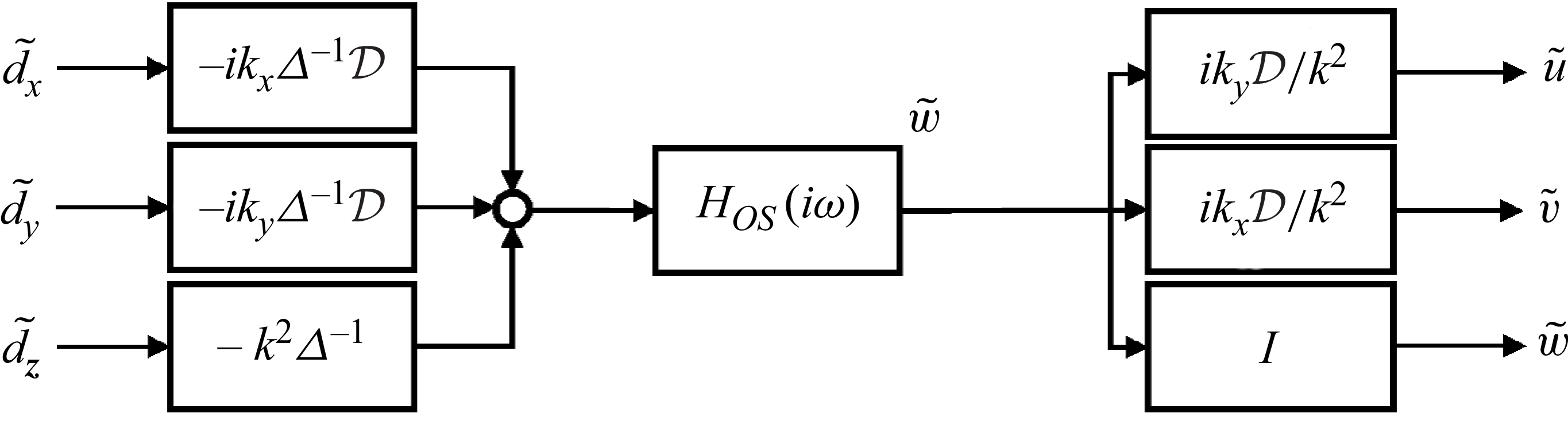
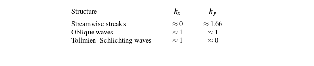
 kx
kx ky
ky
 kx≈1
kx≈1 ky≈±1
ky≈±1 kx
kx ky
ky kx≈1
kx≈1 ky≈1
ky≈1
 log10(‖H‖∞)
 R=2000
 Rτ=2000
 dx~,dy~,dz~
 u~,v~,w~
 log10(‖Hus‖∞)
 R
R s
s d~x,d~y,d~z
 log10(‖Hvs‖∞)
 R
R s
s d~x,d~y,d~z
 log10(‖Hws‖∞)
 R
R s
s d~x,d~y,d~z
 log10(‖HOS‖∞)
 log10(‖HSq−u‖∞)
 log10(‖Hu‖∞)
 R=2000
 dx~,dy~,dz~
 log10(‖HOS‖∞)
 log10(‖HSq−v‖∞)
 log10(‖Hv‖∞)
 R=2000
 dx~,dy~,dz~
 u
u kx=0,ky=1.66
 u
u kx=1,ky=1
 w
w kx=1,ky=0
 log10(‖HOS‖∞)
 log10(‖HSq−u‖∞)
 log10(‖Hu‖∞)
 Re=2000
 x,y,z
x,y,z
 log10(‖HOS‖∞)
 log10(‖HSq−v‖∞)
 log10(‖Hv‖∞)
 Re=2000
 x,y,z
x,y,z
 log10(‖HOS‖∞)
 log10(‖HSq−u‖∞)
 log10(‖Hu‖∞)
 Reτ=2000
 x,y,z
x,y,z
 log10(‖HOS‖∞)
 log10(‖HSq−v‖∞)
 log10(‖Hv‖∞)
 Reτ=2000
 x,y,z
x,y,z
 Open access

