


1. Introduction
Many advances have been made on the theoretical modelling of tidal turbine performance in confined channels. The work of Garrett & Cummins (Reference Garrett and Cummins2007) demonstrated the importance of considering the impact of blockage (flow confinement) on the upper limit of energy extraction for a homogeneously arrayed turbine fence that completely spans the width of the channel under the assumption of an undeforming free surface. This upper limit increases from the Betz limit typically assumed for unconstrained wind turbines in proportion to the square of the relative confinement. Corrections have been applied to tidal turbines to account for the deformation of the free surface (Whelan, Graham & Peiró Reference Whelan, Graham and Peiró2009). Nishino & Willden (Reference Nishino and Willden2012) extended the model by considering a long turbine fence that only partially spans the width of a channel, allowing for incomplete channel use that may be necessitated in practical turbine arrangements, for example due to bathymetric variations or shipping lanes. Here, two scales of flow confinement are considered: a local blockage (ratio of turbine frontal area to local flow passage area) dependent on tip-to-tip spacing between adjacent turbines, and a global blockage effect due to the channel geometry constraints. This model, working on the basis of scale separation between turbine and array scale flow events, located a new energy extraction limit for a closely packed tidal turbine fence in an infinitely wide channel of  $79.8\,\%$ of the kinetic energy flux of the undisturbed approach stream, achieved at a local blockage ${\sim }0.4$. Additionally, the model has been applied to multiple rows of tidal turbines (Draper & Nishino Reference Draper and Nishino2014), where it was found that a single row of turbines outperforms a staggered arrangement, and to shallow channels with non-negligible bed friction, which was found to change both the power extraction potential and the optimum fence arrangement (Creed et al. Reference Creed, Draper, Nishino and Borthwick2017). The scale-separation effect has been demonstrated experimentally using porous discs (Cooke et al. Reference Cooke, Willden, Byrne, Stallard and Olczak2015), and power uplift through the local blockage effect has been shown in large laboratory turbine experiments (McNaughton et al. Reference McNaughton, Cao, Nambiar, Davey, Vogel and Willden2022).
These flow confinement models, however, assume a fixed flow rate through the channel. Garrett & Cummins (Reference Garrett and Cummins2005) developed a channel dynamics model that accounted for the sinusoidally varying channel head as well as the response of the channel flow rate to the resistance presented by the turbines. The tidal turbine farm is modelled as a single modifiable drag (or bed-friction) coefficient in a one-dimensional channel, for which it is found that the maximum power results from a balance between increasing the drag coefficient to increase power production and the associated reduction in channel flow rate that reduces power production. A later extension by Vennell (Reference Vennell2010) allowed for the response of the channel flow rate to the resistance presented by the turbines spanning the entire channel width by taking into account blockage effects predicted by Garrett & Cummins (Reference Garrett and Cummins2007). Additionally, the models have been applied to other problems such as multiple channels (Cummins Reference Cummins2013) and bays connected to oceans (Blanchfield et al. Reference Blanchfield, Garrett, Wild and Rowe2008).
One of the key purposes of these models is to help to determine the tidal stream resource of a tidal channel site. The models provide a well-defined upper bound on the resource, and have been used widely to assess tidal power potential (Sutherland, Foreman & Garrett Reference Sutherland, Foreman and Garrett2007; Karsten et al. Reference Karsten, McMillan, Lickley and Haynes2008; O'Hara & Gallego Reference O'Hara and Gallego2017). However, the models either assume that the turbines occupy the full channel width or rely on numerical approximations. Vennell (Reference Vennell2013) additionally analysed the efficiency of a tidal farm based on an actual site, and found that exceeding the Betz limit needs additional careful consideration of structural load and blockage constraints. Refinements to the upper bound have been considered, with Adcock et al. (Reference Adcock, Draper, Houlsby, Borthwick and Serhadlioğlu2013) locating a new upper-bound estimate for an actual site by numerically considering wake mixing losses, enabling the calculation of the power usefully available for extraction as opposed to the total power removed from the flow.
Whilst these models have significantly improved on the Betz limit for estimating tidal power efficiency, they still fall short of representing realistic turbine physics. In particular, although the Nishino & Willden (Reference Nishino and Willden2012) model does consider finite length fences, and is therefore appropriate for the realistically achievable low global blockages, it is restricted to a constant flow rate through the channel such that the turbine resistance has no influence on the channel dynamics. To address this issue, Gupta & Young (Reference Gupta and Young2017) proposed a quasi-steady theoretical model that combines the short fence extension to the two-scale theory (Nishino & Willden Reference Nishino and Willden2013) with both a free-surface deformation correction and the coupling of added drag with the upstream flow rate. Their flow rate model is based on a simplified static channel model detailed in Bryden & Couch (Reference Bryden and Couch2007). A numerical framework was developed in the work of Bonar et al. (Reference Bonar, Chen, Schnabl, Venugopal, Borthwick and Adcock2019), where the two-scale model was embedded and coupled to realistic rough and oscillatory channel flows, for which the potential power capture was found to be greater as compared to the stand-alone steady-state two-scale model.
This paper presents a simplified analytic model that embeds the multi-scale partial fence model of Nishino & Willden (Reference Nishino and Willden2012) in the channel dynamics model of Garrett & Cummins (Reference Garrett and Cummins2005), drawing on the work of Willden, Nishino & Schluntz (Reference Willden, Nishino and Schluntz2014). The model allows for the analytic consideration of both rough bottom channels and oscillatory flow in a time-dependent framework, extending the work of Gupta & Young (Reference Gupta and Young2017). The model also accounts for the increase in performance due to local and global blockage effects, extending the works of Garrett & Cummins (Reference Garrett and Cummins2005) and Vennell (Reference Vennell2010) to a fence partially spanning the channel width. As the work of Draper & Nishino (Reference Draper and Nishino2014) has shown, for a fixed number of turbines, a single co-planar side-by-side row of turbines outperforms multi-row array arrangements, be they streamwise aligned or staggered; the model presented in this paper is restricted to a single fence of turbines partially spanning the width of a head-driven channel.
2. Finite-fence channel dynamics model
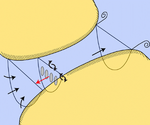
The flow problem is outlined by the sketch in figure 1, in which the flow is driven through the channel by a sinusoidally varying head difference between the channel ends. A turbine fence is positioned such that it partially occupies the width of the channel. The turbine fence consists of a large number  $n$ of closely spaced turbines, each of diameter $d$, that are arrayed with a tip-to-tip separation $s$ in a plane normal to the channel flow direction.
Schematic of a head-driven channel between two large basins in which a tidal turbine fence occupying part of the width of the channel is arrayed normal to the flow direction. An additional close-up view of a section of the fence shows the turbine scale flow problem. Remixing between core and bypass flows is shown for both turbine and fence scales.

The channel is simplified to be of rectangular cross-section with length  $l$, width $w$ and height $h$. The flow is driven by the elevation difference across the channel ends, $\zeta _i(t)-\zeta _e(t)$, which is assumed to vary sinusoidally in time with amplitude $a$ and frequency $\omega$. This forcing could be extended to account for higher-order interactions, for example the difference of sinusoidal tides at the ends of the channel. The resulting flow velocity through the channel is then $U_C(t)=Q(t)/(wh)$, where $Q(t)$ is the flow rate, and both $U_C$ and $Q$ are functions of time alone due to the geometric simplification of constant channel cross-section, and an assumption that the driving tidal wave is far longer than the channel length (as per Garrett & Cummins Reference Garrett and Cummins2005).
The flow through the turbine fence is modelled following the partial fence model of Nishino & Willden (Reference Nishino and Willden2012) in which two scales of flow are considered: device scale flow and array scale flow. At the array scale, the resistance of the turbine fence causes flow diversion, resulting in an approach velocity  $U_A$ to the array that is lower than the stream velocity $U_C$. Similarly, at device scale, the resistance of each individual turbine causes flow to divert around each device such that the flow velocity through each device, $U_D$, is less than the array approach velocity $U_A$. Device scale mixing of device core and bypass flows occurs at dimensions scaling on the device diameter. This completes ahead of array scale mixing of array core and bypass flows, which occurs on dimensions scaling on the fence length. Through kinematic and dynamic coupling of the device, and array scales of the finite fence problem, the Nishino & Willden (Reference Nishino and Willden2012) partial fence model provides a solution to the steady flow through the fence, and thus the power generated by the turbine fence, which may be parametrised conveniently by either turbine fence thrust or induction factor.
The Nishino & Willden (Reference Nishino and Willden2012) partial fence model is a steady flow model and hence assumes implicitly that the upstream mass flux is unaffected by the resistance within the channel, which can be strictly true only at vanishingly small global blockage. By coupling the channel dynamics problem with an assumed quasi-steady partial fence model, the impact of fence resistance on channel flow rate can be incorporated so that the more relevant problem of the performance of a partial fence placed within a head-driven finite global blockage channel can be considered.
2.1. Channel dynamics model
The one-dimensional channel dynamics model of Garrett & Cummins (Reference Garrett and Cummins2005), which can be derived from the one-dimensional Euler equation, may be recast in non-dimensional form (the non-dimensional formulation was first presented in Willden et al. (Reference Willden, Nishino and Schluntz2014) – see Appendix A for a complete derivation) as
 \begin{equation} \frac{{\rm d} Q^\prime}{{\rm d} t^\prime} - \cos t^\prime ={-} \frac12\, Q^\prime\,| Q^\prime |\,\frac{1}{{{Fr}}_\omega^2} \left( B_A C_{TA} + C_f\,\frac{l}{h} \right),\end{equation}
in which the flow is driven through the (here presumed) rectangular cross-section channel by a sinusoidally varying head difference between the ends of the channel. Here,  $Q^\prime =Q/Q_0$ is the non-dimensional flow rate, in which $Q_0={(ga/\omega )}{(wh/l)}$ is the peak volume flow rate in the undisturbed channel (assuming negligible inflow and exit kinetic energy fluxes, and the absence of bed friction). Time $t$ is non-dimensionalised according to $t^\prime =\omega t$. This non-dimensionalisation has been applied previously by Muchala & Willden (Reference Muchala and Willden2017) to investigate the impact of support structure drag on tidal turbine performance. In this model, however, the addition of the $B_A C_{TA}$ group indicates the extension to the internal coupling of the Nishino & Willden (Reference Nishino and Willden2012) model.
The channel entry and exit are assumed smooth so that kinetic fluxes in and out of the channel may be neglected. The model equation (2.1) is an energy balance equation in which all terms are energy losses except for the driving head term  $\cos t^\prime$, which supplies energy to the channel. The unsteady term represents the energy required to accelerate the flow through the channel, whilst the right-hand side represents the energy lost to overcome opposing (resistive) forces.
The resistance to the flow has two contributions: from bed friction, included through the friction coefficient  $C_f$, and due to turbine array thrust, included through the array thrust coefficient
 \begin{equation} C_{TA}={\frac{T_A}{\frac{1}{2} \rho U_C^2 w_A h}},\end{equation}
in which  $T_A$ is the array thrust, $w_A=n{({d+s})}$ is the width of the turbine fence (array) and $\rho$ is the fluid density. The proportion of the channel width occupied by the turbine fence is described by the array blockage ratio
 \begin{equation} B_A=\frac{w_A}{w}.\end{equation}
 The flow characteristics in the empty channel are governed by the non-dimensional groups  ${{Fr}}_\omega$ and $l/h$, and the bed friction $C_f$. Here, ${{Fr}}_\omega = \omega l / \sqrt {g a}$ takes the form of a Froude number and can be shown to be proportional to the square root of the ratio of cycle-averaged head supplied to the kinetic energy in the unresisted channel (see Appendix A). This channel-based Froude number describes the flow rate through the channel: for a fixed-geometry channel, increasing the amplitude of the tidal wave $a$ (and thus decreasing ${{Fr}}_\omega$) leads to an increase in flow rate through the channel, as expected. The product $C_f (l/h)$ provides the overall bed resistance, so increasing the depth of flow (and thus decreasing $l/h$) diminishes the importance of bed friction leading to an increase in the channel flow rate.
Specifying the product  $C_f(l/h)/{{Fr}}^2_\omega$ enables solution of the channel flow problem in the absence of turbines. In the case of a turbine fence installation, we define the channel characteristics through specification of $C_f(l/h)$ and ${{Fr}}_\omega$ separately. The problem is then closed fully by specification of the proportion of the channel width occupied by turbines, $B_A$, and the array thrust coefficient $C_{TA}$, which is provided by kinematic and dynamic coupling to the partial fence model as outlined below. Although the resistive terms in the model equation (2.1) could be presented through two terms and hence two non-dimensional groups, as in Garrett & Cummins (Reference Garrett and Cummins2005), we choose here to use three, namely $C_f(l/h)$, ${{Fr}}_\omega$ and $B_A C_{TA}$, so as to separate properly channel characteristics from turbine characteristics.
Solution of the model equation (2.1) is achieved by time marching. Following several transient cycles, periodic solutions, of period  $2 {\rm \pi}/ \omega$, are obtained over which the time average farm thrust and power may be determined. The periodicity of the solution allows for alternative approaches to solving the model equation, particularly in the frequency domain. These could be considered for cases where rapid solutions are required, or where the phase spectrum is of direct interest. We also note that additional physical mechanisms may potentially increase the time-averaged power above the model predictions, such as dynamic effects following the change in tide direction (Bonar et al. Reference Bonar, Chen, Schnabl, Venugopal, Borthwick and Adcock2019).
2.2. Partial fence model
Specification of the turbine fence thrust as a function of channel flow rate is sufficient to close the problem. Here, we use the partial fence model of Nishino & Willden (Reference Nishino and Willden2012). The turbine fence is taken to lie in a plane normal to the flow direction, and the fence does not fully occupy the width of the channel as required from practical bathymetric and shipping considerations; see figure 1. Hence the array approach flow is divided into an array core stream of velocity  $U_A$, and an array bypass stream. The array core stream may itself be divided into $n$ stream tubes, with each approaching a single device. Each device stream tube may again be divided into a device core stream, with flow speed through the device $U_D=U_A(1-a_L)$, and a device bypass stream. Downstream of the array, we assume a separation of scales between device and array scale mixing. Device scale mixing, between the device core and bypass flows, scales on the device diameter $d$ and occurs ahead of the start of array scale mixing, between the array core and bypass flows, which scales on the length of the array $w_A$. The model assumes implicitly that the fence is sufficiently long (large enough $n$) for this separation to be valid, and that the channel is sufficiently long – multiples of $w_A$ – for array scale mixing to be completed within the channel. The numerical simulations of Nishino & Willden (Reference Nishino and Willden2013) suggest that the restriction on $n$ to achieve scale separation is not particularly onerous, with $n \ge 8$ achieving good agreement between theory and computation.
Each of the inner (device scale) problem and the outer (array scale) problem may be solved by application of the Garrett & Cummins (Reference Garrett and Cummins2007) model of device performance in a blocked flow passage. Their model extends the conservation of linear momentum theory, applied conventionally to unbounded wind turbines in which the outer flow can expand freely, to the case of a device in a finite cross-section flow passage in which the flow can no longer expand in an unconstrained manner. Such a geometric constraint results in the acceleration of the device bypass flow. It is assumed that downstream of the device, the core flow expands and the bypass flow contracts until a point of pressure equilibrium between the two streams is reached, following which the core and bypass flows remix to recover a uniform stream. Unlike the unbounded wind turbine theory, this blocked theory results in a solution in which a favourable pressure gradient is developed between the far upstream and downstream conditions. As in the Garrett & Cummins (Reference Garrett and Cummins2007) blocked device model, we here neglect changes in the free surface elevation and assume that the flow is bounded by a rigid lid. At the channel scale, however, following Garrett & Cummins (Reference Garrett and Cummins2005), we assume a channel depth that varies in time according to the driving tidal wave. Relaxation of the rigid-lid assumption at the device and array scales has a significant impact on only the model predictions for large Froude number ( ${Fr}=U_C/\sqrt {gh}$) channels (Vogel, Houlsby & Willden Reference Vogel, Houlsby and Willden2016) or high global blockage ratios. As Froude numbers for realistic tidal channels are comparatively low ( $0.1\leq {Fr}\leq 0.2$; Vogel et al. Reference Vogel, Houlsby and Willden2016), and the results presented herein show peak performance points at modest global blockage ratios (see § 3), the rigid-lid assumption made in the partial fence model will introduce only small errors for practical turbine array deployment scenarios.
Starting with the inner device scale problem, we use the device scale thrust coefficient  $C_{TL}$ to non-dimensionalise the device scale thrust $T_D$ through
 \begin{equation} C_{TL}={\frac{T_D}{\frac{1}{2} \rho U_A^2 {\rm \pi}d^2/4}} .\end{equation}
Applying the Garrett & Cummins (Reference Garrett and Cummins2007) model to the device scale problem enables this thrust coefficient to be evaluated through
 \begin{equation} C_{TL}={({1-\gamma_L})} {\left[ \frac{ {({ 1+\gamma_L })} - 2 B_L {({1-a_L})} }{ {({ 1 - B_L {({1-a_L})}/\gamma_L })}^2 } \right]} ,\end{equation}
in which  $\gamma _L$ is the ratio of the device scale wake velocity (at the device scale pressure equilibrium location) to the device approach velocity $U_A$, and $B_L$ is the local blockage ratio defined as
 \begin{equation} B_L=\frac{{\rm \pi} d^2 / 4}{{({d+s})} h },\end{equation}
in which the denominator is the cross-sectional area of the device scale flow passage. The ratio of device wake to approach velocity,  $\gamma _L$, is related through mass conservation to the device induction factor $a_L$ through
 \begin{equation} 1-a_L = { \frac{1+\gamma_L}{ {({1+B_L})} + {\sqrt{ {({ 1-B_L})}^2+B_L {({ 1-1/\gamma_L })}^2 }} }}.\end{equation}
Once the local blockage has been specified, (2.5) and (2.7) may be solved for  $C_{TL}$ as a function of $a_L$ alone. For each $0<\gamma _L<1$, (2.7) provides a unique solution $0< a_L<1$, which then solves for a unique $C_{TL}$ in (2.5).
Following Nishino & Willden (Reference Nishino and Willden2012), who first developed this two-scale model, we now apply the Garrett & Cummins (Reference Garrett and Cummins2007) model to the array scale problem, resulting in a similar form of equations that relate the array thrust coefficient  $C_{TA}$ to the array induction factor $a_A$, which itself relates the array approach flow velocity to the channel flow velocity through $U_A=U_C (1-a_A)$. Once the array blockage $B_A$ has been specified, the array thrust $C_{TA}$ is parametrised by $a_A$ as
 \begin{equation} C_{TA}={({1-\gamma_A})} {\left[ \frac{ {({ 1+\gamma_A })} - 2 B_A {({1-a_A})} }{ {({ 1 - B_A {({1-a_A})}/\gamma_A })}^2 } \right]} ,\end{equation}
in which  $\gamma _A$ is the ratio of array wake velocity (at the array scale pressure recovery location) to the upstream channel velocity $U_C$, related to the array induction $a_A$ by
 \begin{equation} 1-a_A = { \frac{1+\gamma_A}{{({1+B_A})} + {\sqrt{ {({ 1-B_A})}^2+B_A {({ 1-1/\gamma_A })}^2 }} }} .\end{equation}
 The device and array problems are coupled kinematically through the array approach velocity  $U_A$, and dynamically through specifying the array thrust to be $n$ times the device thrust, i.e. $T_A=nT_D$, or non-dimensionally,
 \begin{equation} C_{TA}={({1-a_A})}^2 B_L C_{TL} .\end{equation}
 The kinematic and dynamic coupling closes the partial fence problem leading to a solution for array thrust as a function of device induction factor. Each device is assumed to be a perfect energy extractor so that it delivers power  $P_D=T_D U_D$. Once device thrust, and device and array velocities, have been determined, the device local power coefficient $C_{PL}$ and array global power coefficient $C_{PG}$ may be determined trivially from
 \begin{gather} C_{PL} = \frac{P_D}{\frac{1}{2} \rho U_A^3 {\rm \pi}d^2/4 }, \end{gather}
 \begin{gather}C_{PG} = \frac{n P_D}{\frac{1}{2} \rho U_C^3 n {\rm \pi}d^2/4 } = {({ 1-a_A })}^3 C_{PL} . \end{gather}
2.3. Coupled channel partial fence dynamics model
For any given turbine layout, specified through the combination of local blockage  $B_L$, which represents the spacing between turbines, and global blockage $B_G=B_L B_A$ (the ratio of total disc to channel cross-sectional areas), which represents the total number of turbines, the dynamic channel flow problem can be solved as a function of the applied fence thrust $B_A C_{TA}$. The partial fence model provides this non-dimensional group in (2.1) as a function of the array induction factor.
To couple the partial fence model to the channel flow model, we make the assumption that the fence operates at a constant array (or indeed device) induction factor across the entire tidal cycle; that is, we assume that the turbines in the fence operate solely with local knowledge so as to reduce the speed of the approach flow through the turbines by a fixed proportion (the induction factor) – as do wind turbines operating below rated flow speeds. The partial fence model may be solved conveniently in advance of the channel flow problem to provide the fence performance parametrised across the range of array induction factors  $0\leq a_A\leq 1$.
The  ${Fr}_\omega$ and $C_f (l/h)$ groups are set based on the driving tidal wave, and channel geometry and bed friction estimates. Equation (2.1) is then integrated forwards in time until the peak amplitude of the channel flow rate, $\hat {Q}/Q_0$, converges across consecutive cycles. Figure 2 shows an example output $Q/Q_0$ for the peak performance point over two tidal cycles. Across the parameter space, the solution always converges to a periodic waveform, but not necessarily to a single-frequency cosine.
Example solutions to the channel flow rate over two tidal cycles. (a) The solid black line shows the undisturbed flow rate, the dashed line shows the flow rate assuming peak power production with homogeneous resistance in the Garrett & Cummins (Reference Garrett and Cummins2005) model and the solid red line shows the coupled fence–channel model flow rate for a specified fence geometry. (b) For a specified arrangement of turbines, the relationship between the peak flow rate reduction and the channel thrust and power coefficients. The peak power point locates the optimal thrust and necessary flow reduction for the specified arrangement.

The solution presents in terms of a fence performance, which we assess through the cycle-averaged channel-based power coefficient  $C_{PC}$ across the range of array induction factors $a_A$, with each induction factor corresponding to an applied global thrust coefficient $C_{TG}$ defined by
 \begin{equation} C_{TG} = \frac{C_{TA}}{B_L}, \end{equation}
which acts to reduce the amplitude of the flow rate by a factor  $\hat {Q}/Q_0$. The thrust and power coefficients normalised by the peak channel flow rate (consistent with Garrett & Cummins Reference Garrett and Cummins2005) are defined by
 \begin{gather} C_{TC} = \frac{n\,T_{D{,max}}}{\rho g a A_C}, \end{gather}
 \begin{gather}C_{PC} = \frac{n\,\overline{P_D}}{\rho g a Q_0} , \end{gather}
where the overbar denotes a time average over a complete period of the driving tidal wave, and  $T_{D,max}$ is the peak thrust over a tidal period.
As the channel thrust is increased, the flow rate through the channel is reduced (figure 2b). There is a consequent variation in the channel power, which at first increases until a peak performance is reached, before reducing as the channel flow rate is reduced too aggressively. This paper focuses on these optimal extraction points, which are unique for each set of turbine arrangements  $(B_L,B_G)$. Finally, we here define $C_{TD}$ to be the peak single disc thrust
 \begin{equation} C_{TD}=\frac{T_{D,{max}}}{\rho g a A_T} = \frac{C_{TC}}{B_G}, \end{equation}
as a metric to assess peak turbine loads. We assume that the channel and turbine peak resistances  $C_{TC}$ and $C_{TD}$ are constant from cycle to cycle.
The partial fence formulation is the precursor step that provides one of the inputs to the channel dynamics model, and the two models may be conveniently solved sequentially. In discussion of model results, for each  $B_G$ and $B_L$, we concentrate on the fence thrust that results in the maximum $C_{PC}$ as being the solution of interest to the channel–fence problem. To then map the performance over a range of $B_L$ and $B_G$, this process may be repeated for $B_G\leq B_L\leq 1$, $0\leq B_G \leq B_L$. In the absence of additional bed friction, the assumptions underpinning the limiting case as $B_L,B_G \to 1$ converge to the Garrett & Cummins (Reference Garrett and Cummins2005) channel model. In all cases where $C_f=0$, the homogeneous array ( $B_L,B_G \to 1$) flow rate reduction therefore approaches near $\hat {Q}/Q_0=2^{-1/2}$, and peak power approaches $C_{PC}=0.24$ (see, for example, figures 3(a) and 3(c), and the Garrett & Cummins (Reference Garrett and Cummins2005) homogeneous fence solution).
Contours of fence performance for  ${Fr}_\omega =0.635$, $C_f=0$, $l/h$ undefined. All presented solutions correspond to the array thrust setting that achieves maximum $C_{PC}$ at the indicated combination of blockage ratios. The black circle represents the maximum return point, and the red dashed line indicates the locus of $\hat {Q}/Q_0=0.95$. The dashed lines provide geometric limits on blockages for ratios of channel height $h$ to turbine diameter $d$. (a) The channel power coefficient, with the solid black line indicating the locus of maximum $C_{PC}$ with global blockage; (b) the return parameter; (c) the normalised peak flow rate; (d) the peak return, peak power coefficient and corresponding channel thrust across contours of normalised peak flow rate; (e) the disc thrust coefficient; (f) the basin efficiency.

3. Finite fence performance in a head-driven channel
To contextualise the model results, we first consider typical tidal channel dimensions presented in table 1 (taken from Vennell & Adcock Reference Vennell and Adcock2014), from which realistic ranges of the non-dimensional groups can be determined readily. As a reference case, we first consider a channel with a  ${Fr}_\omega$ value between that of the two example channels listed in table 1. We then vary ${Fr}_\omega$ and consider the impact of bed friction assuming a typical bed-friction coefficient $C_f=0.002$ across channel $l/h$ ratios spanning the typical geometric ranges observed.
Example channel dimensions based on a hypothetical small channel and the Pentland Firth.

3.1. Zero bed friction reference case
An example solution for the head-driven array model is shown in figure 3 to demonstrate the impact of blockage on the fence performance in a channel with coupled upstream flow. This reference case is within the range of practical interest; we take lunar frequency  $\omega = 1.4\times 10^{-4}$ rad s $^{-1}$, equivalent to the dominant lunar $M_2$ frequency, and assume tidal amplitude $a=0.5$ m, tidal turbine diameter $d=20$ m, and channel length $l=10$ km, resulting in a channel Froude number ${Fr}_\omega = 0.635$. For now, we assume that the channel bed friction $C_f$ is negligible, but compare against cases with non-zero bed friction in § 3.3.
The channel power coefficient  $C_{PC}$, contoured in figure 3(a), increases with increasing global blockage. For any given global blockage (or specified flow reduction factor $\hat {Q}/Q_0$), there exists a corresponding $B_L$ to maximise power generation, much as in the steady flow partial fence model (Nishino & Willden Reference Nishino and Willden2012). The physics of this increase in extractable power by local and global blockage mechanisms is discussed in detail in Dehtyriov et al. (Reference Dehtyriov, Schnabl, Vogel, Draper, Adcock and Willden2021). We additionally define the return parameter
 \begin{equation} R = \frac{C_{PC}}{B_G}\propto \frac{\textrm{total power extracted}}{\textrm{total frontal turbine area}}, \end{equation}
which may be interpreted usefully as income (power generated) per cost (turbine area). The maximum return, and the corresponding optimal turbine layout ( $B_L$ and $B_G$), can be determined from the model. Figure 3(b) shows the contours of the return parameter for the reference flow case, with the optimum indicated. For large channels where the turbine fence is expected to occupy a small proportion of the channel cross-section ( $B_G\to 0$), there remains an optimal spacing $B_L$ to maximise return. Increasing $B_G$ then increases the peak return at a new optimal $B_L$, with the largest return ratio in this case realised for $B_G\approx 0.18$, $B_L\approx 0.49$. Further increases in $B_G$ then allow higher levels of achievable channel power $C_{PC}$ at the cost of a lower return, i.e. there are diminishing benefits from adding more turbines.
Furthermore, there may exist maximum permissible flow rate reductions, as shown by the contours in figure 3(c), due to environmental constraints for which a typical limit is  $\hat {Q}/Q_0=0.95$ (The Carbon Trust 2011). For the reference case, the maximum return falls just within this assumed environmental constraint; however, careful consideration of the environmental impact is necessary for layout design where the optimal return requires larger attenuation of flow rate. For a quantified understanding, figure 3(d) plots the maximum return and channel power coefficients, together with the channel thrust coefficient at which these occur, along contours of the maximum allowable flow reduction. As the constraint is tightened, channel power and thrust fall monotonically (tending to zero as $\hat {Q}/Q_0\to 1$), but the optimal return is here realised for $\hat {Q}/Q_0=0.95$, and movement away from this optimum decreases the return. Therefore, all else being equal, tightening of the constraint (i.e. reducing flow rate impact) requires the turbine layout to be changed, with reductions in both global blockage (fewer turbines) and local blockage (more spaced out) in order to maximise return and power.
At this optimal return point, the local blockage is relatively high, and the optimal induction factor to maximise the channel power coefficient increases when compared to unblocked and blocked flow models at the same global blockage (Garrett & Cummins Reference Garrett and Cummins2007). Similar to the two-scale and blocked flow models, this leads to a larger peak operating disc thrust coefficient shown in figure 3(e), which needs to be further accounted for in the design of the turbine structure. The root-mean-square thrust can be estimated by dividing the peak thrust by  $\sqrt {8/3}$, but, depending on the global blockage, it is likely that power capping control strategies will still be required by real turbines to limit the maximum thrust whilst operating at the optimal flow reduction factor as suggested by Vogel, Willden & Houlsby (Reference Vogel, Willden and Houlsby2019). For instance, figure 4 shows how a controlled reduction in the thrust at the optimal design point for maximising return would impact the return. An example $20\,\%$ de-rating from the peak thrust point would decrease the return by only $5\,\%$. Furthermore, such thrust capping may also be necessary only at near peak flow speeds.
The impact of varying the peak disc thrust coefficient  $C_{TD}$ on the return parameter at the optimal design ( $B_L,B_G$) point for the reference flow case shown in figure 3. The impact on return of a $20\,\%$ de-rating of the thrust is also shown.

Additionally, an increase in extractable power due to non-zero local blockage results in a decrease in the basin efficiency  $\eta$, the ratio of power extracted by the turbines to the total power removed from the flow (figure 3f) – with the latter necessarily exceeding the former due to the energy lost in wake remixing processes. A minimum allowable basin efficiency could be considered as an additional constraint for optimisation of the return. Here, it is useful to note that a Betz-optimum unblocked wind turbine operates with basin efficiency $2/3$, so for the model parameters set in this reference case, the efficiency of extraction (basin efficiency) does not fall far below the unblocked optimum ( $\eta =0.59$ for maximum return).
Finally, we note that the maximum local blockage is constrained by the depth of the channel. In this case, the optimal return is realised for  $(h/d)_{{max}} \approx 1.5$. For the assumed turbine diameter $d=20$ m, the channel depth is therefore bounded by $h\leq 30$ m to achieve this optimal blockage ratio in a fence configuration. For deeper channels, alternative non-single-row fence arrangements of turbines are hence necessary to optimise return.
Of further interest is how variations in the channel parameters affect the optimal turbine configuration. In §§ 3.2 and 3.3, we hence consider variations in the non-dimensional groups governing the channel characteristics, namely the channel Froude number  ${Fr}_\omega =\omega l/\sqrt {a g}$, and the channel friction parameter $C_f (l/h)$.
3.2. Effect of variation in channel Froude number
The channel-based Froude number can be interpreted physically as proportional to the square root of the ratio of cycle-averaged driving head to kinetic head (see Appendix A). Therefore, for a fixed driving head, the kinetic head decreases with increasing Froude number, and we might expect a lower return. Figures 5 and 6 illustrate the impact of the channel Froude number on both the fence performance and the environmental impact, respectively. Here, we consider two simple changes to the reference channel flow case. In figures 5(a,c,e) and 6(a,c,e), we assume that the tidal range has risen to  $a=0.8$ m such that ${Fr}_\omega =0.5018$ (for the same channel dimensions and tidal frequency), and in figures 5(b,d,f) and 6(b,d,f) we assume that the tidal range has fallen to $a=0.2$ m such that ${Fr}_\omega =1.004$.
Contours of fence performance comparing (a,c,e)  ${Fr}_\omega =0.5018$, and (b,d,f) ${Fr}_\omega =1.004$, all for $C_f=0$ and $l/h$ undefined. All presented solutions correspond to the array thrust setting that achieves maximum $C_{PC}$ at the indicated combination of blockage ratios. The black circle represents the maximum return point, and the red dashed line indicates a locus of $\hat {Q}/Q_0=0.95$. The dashed lines provide geometric limits on blockages for ratios of channel height $h$ to turbine diameter $d$. (a,b) The channel power coefficient, with the solid black line indicating the locus of maximum $C_{PC}$ with global blockage; (c,d) the return parameter; (e,f) the disc thrust coefficient.

Contours related to channel environmental constraints for (a,c,e)  ${Fr}_\omega =0.5018$, and (b,d,f) ${Fr}_\omega =1.004$, with $C_f=0$ and $l/h$ undefined. All presented solutions correspond to the array thrust setting that achieves maximum $C_{PC}$ at the indicated combination of blockage ratios. The black circle represents the maximum return point, and the red dashed line indicates the locus of $\hat {Q}/Q_0=0.95$. The dashed lines provide geometric limits on ratios of channel height $h$ to turbine diameter $d$. (a,b) The normalised flow rate; (c,d) the peak return, peak channel power coefficient and corresponding channel thrust coefficient across contours of normalised flow rate; (e,f) the basin efficiency.

For a fixed global blockage or relative flow rate, there remains an optimal local blockage to maximise the channel power coefficient. However, an increase in channel Froude number for fixed  $B_G$ causes the channel power coefficient to decrease (figures 5a and 5b). For example, in this case for $B_G=0.2$, $C_{PC}$ falls $\sim 64\,\%$ through the increase in ${Fr}_\omega$ considered. Interestingly, for either fixed $B_G$ or $\hat {Q}/Q_0$, the optimal spacing $B_L$ for maximising $C_{PC}$ between the two cases does not change. For a fixed number of turbines or fixed environmental constraints, therefore, the channel dynamics impacts only the resultant power output and not the optimal configuration.
By contrast, both the magnitude and location of the maximum return vary significantly with variation in  ${Fr}_\omega$ (figures 5c and 5d). The magnitude of the optimal return increases with decreasing channel Froude number, and is realised at both lower local blockage and global blockage. This is particularly important when considering constraints on the flow reduction, with high ${Fr}_\omega$ channels necessitating a larger move away from the optimum under the same constraint (here plotted for $\hat {Q}/Q_0=0.95$). Similar to the reference flow case, as well as the two-scale and blocked flow models, an increase in the return can be correlated broadly to an increase in the disc thrust coefficient (figures 5e and 5f), with peak $C_{TD}$ of the low ${Fr}_\omega$ case more than three times larger than the high ${Fr}_\omega$ case. Turbines will therefore need to be designed carefully for the specific channel dynamics, and both channel and turbine fence configuration selection are critical for optimal return at a given site.
Figure 6 details the environmental impact of turbines operating in channels of varying  ${Fr}_\omega$. The decreases in $C_{PC}$ with increasing ${Fr}_\omega$ observed in figure 5 correspond to smaller environmental impacts, so the gradients with respect to the global blockage ratio of both the relative flow rate (figures 6a and 6b) and basin efficiency (figures 6e and 6f) are likewise smaller. For high ${Fr}_\omega$ channels, the larger $B_G$ and $B_L$ necessary to maximise return and increase channel power $C_{PC}$ are therefore more attainable due to reduced environmental impact. However, for a given flow rate constraint, the maximum return moves further outside of the constraint envelope as ${Fr}_\omega$ increases. This is quantified in figures 6(c) and 6(d), where for the large ${Fr}_\omega$ case, the maximum return continues to rise with further relaxation of the constraints to $\hat {Q}/Q_0=0.85$, whilst for the low ${Fr}_\omega$ case, peak return is achieved at minimal environmental impact ( $\hat {Q}/Q_0\approx 0.98$). Note that although the lower ${Fr}_\omega$ case achieves its maximum return at reduced environmental impact, the power delivered, $C_{PC}$, is itself lower than in the higher ${Fr}_\omega$ case.
A final consideration for optimising channels with high  ${Fr}_\omega$ is that as the optimal blockage ratio increases, the maximum allowable channel depth for a single-row turbine fence configuration falls. For turbines operating in high-Froude-number channels with large depths, interlaced co-planar multi-row arrangements of turbines are a more likely design consideration for optimal energy extraction.
3.3. Effect of channel bed friction
We now turn our attention to the effect of  $C_f (l/h)$ on both the environmental constraints and array performance. To allow for a clear comparison, the bed-friction coefficient is assumed to be $C_f=0.002$, and we present the results for the reference case channel Froude number ${Fr}_\omega =0.635$. As $C_f (l/h)$ appears combined as a non-dimensional group in (2.1), any change in $l/h$ for a fixed bed friction and fixed channel Froude number is equivalent to holding $l/h$ constant and varying $C_f$ by the same amount. It is also useful to interpret increasing $l/h$ with ${Fr}_\omega$ and $C_f$ fixed as a reduction in channel depth, which should increase the significance of bed friction in the dynamical balance equation. Bed friction and turbine resistance compete with each other to resist the flow, hence for a fixed global blockage (and non-zero bed friction), increases in $l/h$ increase the bed resistance, leading to reductions in the performance of the tidal fence.
Figure 7 illustrates this decrease in channel power with increasing  $C_f (l/h)$. For instance, for $B_G=0.2$, $C_{PC}$ falls by close to $50\,\%$ with an increase in $l/h$ from $50$ to $500$. As with changes in ${Fr}_\omega$, the $C_{PC}$ locus does not vary with changes in $C_f (l/h)$, suggesting that this locus is universal. A curve fit shows that
 \begin{equation} B_L=\frac{9B_G+4}{3B_G+10} \end{equation}
is a good approximation to estimating the turbine spacing required to maximise power depending on the achievable level of global blockage. We also note that in all cases, the maximum return lies on this locus, but may occasionally lie outside of the acceptable environmental constraint envelope. As  $B_G\to 0$, the optimum local spacing is $B_L\to 0.4$, which recovers the local blockage for maximum power found in the partial fence model without channel flow interaction (Nishino & Willden Reference Nishino and Willden2012).
Contours of the channel power coefficient  $C_{PC}$ for ${Fr}_\omega =0.635$ and $C_f=0.002$, comparing differences in the impact of bed friction by varying $l/h$. All presented solutions correspond to the array thrust setting that achieves maximum $C_{PC}$ at the indicated combination of blockage ratios. The black circle represents the maximum return point, and the red dashed line indicates the locus of $\hat {Q}/Q_0=0.95$. The dashed lines provide geometric limits on blockages for ratios of channel height $h$ to turbine diameter $d$: (a) $l/h=50$, (b) $l/h=100$, (c) $l/h=250$ and (d) $l/h=500$.

The return is shown in figure 8, where we observe that compared to variations in  ${Fr}_\omega$, the blockage ratios required to achieve peak return do not vary nearly as strongly. Although the optimal return decreases monotonically with increasing $l/h$, the location of the optimal return does not, due to nonlinearity of the governing equation, occurring first at decreasing $B_G$ up to $l/h=250$ before at increasing $B_G$ for $l/h=500$. The magnitude of the optimal return is impacted significantly by frictional losses. Additionally, as the integrated bed friction increases, the gradient of the return decreases, and near maximum returns can be realised across a large range of $B_L$ and $B_G$. Approximately optimal returns can be achieved across a broad range of blockages whose bed friction is significant. By contrast, the low ${Fr}_\omega$ zero bed friction channel (see figure 5c) has a steep return gradient, and careful consideration of blockage is necessary to optimise return.
Contours of the return parameter  $R$ for ${Fr}_\omega =0.635$ and $C_f=0.002$, comparing differences in the impact of bed friction by varying $l/h$. All presented solutions correspond to the array thrust setting that achieves maximum $C_{PC}$ at the indicated combination of blockage ratios. The black circle represents the maximum return point, and the red dashed line indicates the locus of $\hat {Q}/Q_0=0.95$. The dashed lines provide geometric limits on blockages for ratios of channel height $h$ to turbine diameter $d$: (a) $l/h=50$, (b) $l/h=100$, (c) $l/h=250$ and (d) $l/h=500$.

The nominal flow rate  $Q_0$, which for $C_f (l/h)>0$ is defined to be the channel flow rate without turbines but with bed friction, naturally decreases significantly with increasing bed friction; however, the normalised flow rate $\hat {Q}/Q_0$ shown in figure 9 is not impacted significantly. This stands in contrast to variations in ${Fr}_\omega$, and implies that an increase in the bed friction does not significantly change the environmental constraints on permissible blockage ratios. For high bed-friction channels, design for large blockage ratios to maximise $C_{PC}$ will be highly constrained by flow rate considerations, principally due to the flow rate reduction caused by the bed friction itself. These observations are consistent with Vennell (Reference Vennell2013) and Vennell et al. (Reference Vennell, Funke, Draper, Stevens and Divett2015), who observed diminishing returns for additional turbines in channels with high relative bed friction.
Contours of the normalised flow rate  $\hat {Q}/Q_0$ for ${Fr}_\omega =0.635$ and $C_f=0.002$, comparing differences in the impact of bed friction by varying $l/h$. All presented solutions correspond to the array thrust setting that achieves maximum $C_{PC}$ at the indicated combination of blockage ratios. The black circle represents the maximum return point. The dashed lines provide geometric limits on blockages for ratios of channel height $h$ to turbine diameter $d$: (a) $l/h=50$, (b) $l/h=100$, (c) $l/h=250$ and (d) $l/h=500$.

3.4. Designing for maximum return
Horizontal slices through the return contours at the global blockages for maximum return and for globally unblocked channels are shown in figure 10. For a given set of non-dimensional channel groups, there is always a local blockage  $B_L$ that maximises return, and homogeneous spacing that does not exploit the local blockage effect decreases the return in all cases. As the channel Froude number decreases, the optimal global blockage for maximum return falls (figure 10a), and the local blockage effect becomes the primary mechanism for increases in the return. For globally unblocked channels, the local blockage for peak return is identical to the maximum power found in the partial fence model without channel flow interaction (Nishino & Willden Reference Nishino and Willden2012), and is lower than optimally blocked channels at the same channel Froude number. The maximum return must, however, be de-rated for increases in the channel bed friction (figure 10b), and for particularly high bed-friction channels, a relatively low maximum return is realised at high global blockage, making such channels difficult to optimise and exploit.
Slices (at constant  $B_G$) across contour maps of the return at the required global blockage ratio for maximum return (solid lines) and for globally unblocked channels (dashed lines) for which each curve shows a distinct peak with local blockage. (a) Plots show how variations in the channel Froude number impact the arrangement for maximising return. The optimal global blockage ratios for peak return are $B_G=0.07$ for ${Fr}_\omega =0.502$, $B_G=0.17$ for ${Fr}_\omega =0.635$ and $B_G=0.50$ for ${Fr}_\omega =1.004$. (b) Plots show how variations in the bed friction impact the optimal return arrangement, here for ${Fr}_\omega =0.635$ and $C_f=0.002$. The optimal global blockage ratios for peak return are $B_G=0.11$ for $l/h=50$, $B_G=0.07$ for $l/h=100$ and $B_G=0.21$ for $l/h=500$.

The interplay between these two non-dimensional groups and the maximum return is illustrated in figure 11, where the convergence of the zero global blockage and global blockage for peak return for low  ${Fr}_\omega$ is illustrated. The universality of the optimal $C_{PC}$ locus, and the fact that the maximum return must always lie on this curve, imply that figure 11(b) and (3.2) can be used to specify the number ( $B_G$) and spacing ( $B_L$) of turbines to optimise return for low bed-friction channels at a given ${Fr}_\omega$. The required local and global blockages are illustrated in figure 11(b) as a function of ${Fr}_\omega$. This figure gives a simple look-up for $B_G^*$ and $B_L^*$ as a function of ${Fr}_\omega$ for $C_f(l/h)=0$, which should be very useful for an engineer.
Impact of channel scale non-dimensional groups, the channel Froude number  ${Fr}_\omega$ and the channel bed friction $C_f (l/h)$ on the maximum return point. In all plots, the solid line represents the solution for non-zero global blockage; where appropriate, the dashed line represents zero global blockage. For the case of zero bed friction $C_f=0$, $l/h$ undefined, (a) shows the optimal return for non-zero global blockage (solid line) with the corresponding optimal global blockage (black) and local blockage (red) presented in (b). Here presented for the ${Fr}_\omega =0.635$, $C_f=0.002$ case, (c) shows the optimal return across varying $l/h$ ratios for non-zero global blockage (solid line) with the corresponding optimal global blockage presented in (d).

For channels with non-negligible bed friction (in this case for  $l/d\geq 50$ with $C_f=0.002$), the optimal return can be approximated by linearly de-rating the return from the zero friction case (figure 11c). The dependency of the return on the optimal blockage is, however, non-monotonic (figure 11d), and the turbine layout can be fine-tuned for optimal return by altering $B_G$. However, recall that the gradients of return with blockage are small for non-zero friction cases, so the optimal returns for globally unblocked and blocked channels lie close together for a wide range of $C_f (l/h)$; hence although an optimum global blockage exists, the return remains rather insensitive to it.
We summarise by including a simple dimensional design example for a new tidal array. Suppose that we wish to install turbines with diameter  $d=20$ m in a tidal channel that is $l=8$ km long, $h=30$ m deep and $w=4$ km wide, with driving head amplitude $a=0.5$ m. For an initial estimate, assume an idealised channel with no bed friction. First, find the channel-based Froude number ${Fr}_\omega =\omega l /\sqrt {ga}\approx 0.5$, where we have assumed that the tidal forcing frequency $\omega =1.4\times 10^{-4}$ rad s $^{-1}$ is equal to the dominant lunar $M_2$ frequency. Reading from figure 11(b), the optimal blockage ratios are then $B_G^*\approx 0.08$ and $B_L^*\approx 0.46$. The number of turbines for optimal deployment is then $n=w h B_G/({\rm \pi} d^2/4)\approx 30$. The local blockage $B_L=({\rm \pi} d^2/4) / (h(d+s))$ can then be used to calculate the required tip-to-tip spacing $s$ between each turbine such that $s={\rm \pi} d^2/(4 h B_L) - d\approx 2.8$ m. For this example channel, therefore, a fence of $30$ turbines of diameter $d=20$ m spaced $s=2.8$ m apart for a total fence width $w_A\sim n(d+s) = 684$ m, representing approximately $17\,\%$ the entire width of the channel, is the optimal configuration. The expected return can be read from figure 11(a) at $R^*\approx 0.7$, for a channel power coefficient of $C_{PC}=R^* B_G^* = 0.056$. To estimate the power output, first find the peak undisturbed flow rate $Q_0=(ga/\omega )(wh/l)\approx 526\,000$ m $^3$ s $^{-1}$. The optimal time-averaged turbine array power output for the channel is then $n\overline {P_D}=\rho g a Q_0 C_{PC} \approx 144$ MW, with each individual turbine generating $\overline {P_D}=144/30=4.8$ MW. For detailed solutions that take flow rate and thrust constraints into account, as well as layout optimisation for sites with non-negligible bed friction, a solution of the governing equation as outlined in § 2 is recommended.
4. Conclusions
A theoretical model has been proposed to quantify the efficiency of an array of turbines that partially span the width of a tidal channel in which the flow is driven by a sinusoidally oscillating head. The framework for this analysis is the two-scale finite fence approach (Nishino & Willden Reference Nishino and Willden2012) embedded within and coupled to the one-dimensional channel dynamics model of Garrett & Cummins (Reference Garrett and Cummins2005). The model hence accounts for both the beneficial constructive interference between turbines in fences that partially span the channel width as well as the coupling between turbine resistance and flow rate, and is an extension of previous models by considering both rough bottom channels and time-dependent oscillatory flow. The model makes no additional assumptions beyond those used in the two models from which it is derived, and the solutions to the non-dimensional equation governing the model are presented. We do note, however, the importance of scale separation assumptions for the combined analytic model. We assume that the device scale mixing takes place much faster relative to the array scale mixing, but that the flow rate through the channel is constant along the length of the channel at any given point in time, and hence that the driving tidal wave is longer than the channel length, which must be considerably larger than the array mixing length scale.
Three non-dimensional groups are shown to fully characterise the flow problem: the channel Froude number group  ${Fr}_\omega =\omega l/\sqrt {g a}$, representing the relative (for a given channel length) oscillatory tidal elevation difference between the two ends of the channel (proportional to the square root of the cycle-averaged potential to kinetic head in the channel); the channel bed-friction group $C_f(l/h)$; and the turbine characteristics group $B_A C_{TA}$. This paper explores the impact of these three groups on both the channel scale flow dynamics and turbine performance characteristics. We introduce the return parameter $R$, the maximum yield per turbine area, proportional to a ratio of the total power extracted to the total frontal area of the turbines, as an optimisation metric for the arrangement of turbines in a channel. For a given set of channel parameters, which specify the channel Froude number and bed-friction non-dimensional groups, there is an optimal number ( $B_G$) and arrangement ( $B_L$) of turbines to maximise return. By then further considering environmental constraints on the limiting values of acceptable reductions in relative flow rate, basin efficiency and thrust coefficient, we quantify the optimisation envelope for tidal turbine layouts.
We find that blockage plays a major role in the performance of a tidal farm operating in a head-driven flow, with flow reduction in the channel, return parameter and turbine performance strongly influenced by the different scales of blockage. For even relatively unblocked tidal farms, and especially for optimally arranged tidal farms, modelling the channel flow dynamics and resistance is crucial for farm yield estimation. To gain the full benefit of blockage, turbines and their layouts must therefore be carefully designed for their intended blockage environment.
In general, the channel Froude number  ${Fr}_\omega$ heavily constrains the maximum possible return, and both channel power and the optimal return decrease as ${Fr}_\omega$ is increased. Increasing ${Fr}_\omega$, proportional to the square root of cycle-averaged potential to kinetic head, requires high blockage arrangements to extract at optimal power. Increases in the channel bed friction act to decrease the achievable channel power coefficient and to decrease the peak return. Further, increasing bed friction renders sensitivity of flow rate reduction and return optima on local and global blockage ratios less significant. In all cases, the optimal channel power coefficient lies along a universal curve approximated by $B_L=(9B_G+4)/(3B_G+10)$, with the maximum return moving along this curve as the channel Froude number and channel bed friction are varied.
Both environmental and engineering constraints heavily restrict the operational envelope of the tidal fence. In general, with increases in Froude number, the channel environmental constraint becomes more restrictive and the device thrust constraint becomes less restrictive. For thrust coefficients that are larger than achievable by conventional rotors, power capping control strategies are critically important, particularly at peak flow speeds.
This model has great practical potential in aiding tidal turbine developers with detailed knowledge of the channel and frictional characteristics of a candidate site, resulting in a design envelope including both environmental/peak load constraints and the maximum yield point for optimisation in a head-driven tidal channel. The model is also readily applicable to power-limit estimates for resource assessment, and can further be combined with real turbine characteristics to more accurately predict turbine, as opposed to optimal disc, performance.
Acknowledgements
For the purpose of Open Access, the authors have applied a CC BY public copyright licence to any author accepted manuscript (AAM) version arising from this submission.
Funding
This research was funded in part by D.D.'s EPSRC studentship (grant no. EP/S023801/1), C.R.V.'s UKRI Future Leaders Fellowship (grant no. MR/V02504X/1) and R.H.J.W.'s EPSRC Advanced Fellowship (grant no. EP/R007322/1), and by the EPSRC Supergen ORE Hub (grant no. EP/S000747/1).
Declaration of interests
The authors report no conflict of interest.
Appendix A. Non-dimensionalised channel dynamics governing equation
We start with the Garrett & Cummins (Reference Garrett and Cummins2005) model equation, which comes directly from the streamwise integration of the one-dimensional Euler equation
 \begin{equation} c\,\frac{{\rm d}Q}{{\rm d}t}-ag\cos{\omega t} ={-}\int_0^l F\,{{\rm d} x} , \end{equation}
in which we have assumed smooth inflow and outflow so that the kinetic energy fluxes may be neglected. We assume that the channel cross-section is constant such that  $c=\int _0^l A^{-1}\, {{\rm d} x}=l/A_C$.
Here,  $F$ is the total resistive force per unit mass, which may be distributed arbitrarily along the channel length. The force of the turbines is given by
 \begin{equation} F_T = \tfrac{1}{2}\rho U_C^2 A_C C_{TC} = \tfrac{1}{2}\rho U_C^2 A_C C_{TA} B_A , \end{equation}
and the bed shear stress is given by
 \begin{equation} \tau_b = \tfrac{1}{2} \rho U_C^2 C_f, \end{equation}
which, integrated over the bed surface, gives the resistive force due to bed friction:
 \begin{equation} F_b = \tau_b A_b = \tau_b A_C\,\frac{l}{h} = \frac{1}{2}\,\rho U_C^2 A_C\, \frac{l}{h}\,C_f . \end{equation}
The total force per unit mass  $F$ (where $\rho A_C l$ is the mass of fluid in the channel) is therefore
 \begin{equation} F = \frac{1}{\rho A_C l}\left(\frac{1}{2}\,\rho U_C^2 A_C C_{TA} B_A + \frac{1}{2}\,\rho U_C^2 A_C\,\frac{l}{h}\,C_f\right) , \end{equation}
and substituting this into (A1) gives
 \begin{equation} \frac{{\rm d}Q}{{\rm d}t} = \frac{ag}{c}\cos{\omega t} -\frac{1}{\rho A_C c}\left(\frac{1}{2}\,\rho U_C^2 A_C C_{TA} B_A + \frac{1}{2}\,\rho U_C^2 A_C\, \frac{l}{h}\,C_f\right) , \end{equation}
which results in the channel equation including arbitrary resistance from turbines and bed shear.
By non-dimensionalising with  $t'=t\omega$, $Q'=Q/Q_0$, where $Q_0 = {ga} / ({\omega }) (wh/l) = ga / \omega c$, this simplifies to
 \begin{equation} \frac{{\rm d}Q'}{{\rm d}t'} = \cos(t') - \frac{U_C^2}{2ga}\left(C_{TA} B_A + C_f\,\frac{l}{h}\right) , \end{equation}
and as by definition  $Q=U_C A_C$ so $U_C = Q/A_C = Q' ({ga} / {\omega c A_C})$, we can write
 \begin{equation} \frac{{\rm d}Q'}{{\rm d}t'} = \cos(t') - Q'^2\,\frac{ga}{2\omega^2 l^2}\left(C_{TA} B_A + C_f\,\frac{l}{h}\right) . \end{equation}
Defining a non-dimensional channel Froude number as  ${Fr}_\omega = \omega l /{\sqrt {g a}}$, this can be rewritten as the non-dimensional model equation
 \begin{equation} \frac{{\rm d}Q'}{{\rm d}t'} = \cos(t') - \frac{1}{2}\, Q'^2\,\frac{1}{{Fr}_\omega^2}\left(C_{TA} B_A + C_f\, \frac{l}{h}\right) , \end{equation}
which is the form of the non-dimensional equation first presented in Willden et al. (Reference Willden, Nishino and Schluntz2014), solved for in this paper.
Equation (A1) carries units of energy per unit mass, so the cycle-averaged energy supplied to the channel by the driving head is given by
 \begin{equation} \bar{E}_\zeta = \frac{1}{T} \int_0^T | a g \cos{\omega t} |\, \rho A_C l \,{\rm d}t = \frac{{2\rho l^2 \omega}}{{\rm \pi}}\,Q_0 , \end{equation}
where  $T=2{\rm \pi} /\omega$ is the cycle period. Similarly, in the absence of flow resistance so that $Q = Q_0 \sin {\omega t} = A_C U_C$, the cycle-averaged channel kinetic energy is given by
 \begin{equation} \bar{E}_k = \frac{1}{T} \int_0^T \frac{1}{2}\,\rho A_C l U_C^2 \, {\rm d}t = \frac{{\rho l}}{{4 A_C}}\,Q_0^2, \end{equation}
so the channel-based Froude number
 \begin{equation} {Fr}_\omega = \sqrt\frac{\rm \pi}{8} {\left(\frac{\bar{E}_\zeta}{\bar{E}_k }\right)}^{1/2} \end{equation}
may be interpreted usefully as being proportional to the square root of the ratio of the cycle-averaged driving head to kinetic head in the channel.


 Open access