


1. Introduction
The skin-friction coefficient is the dimensionless wall shear stress exerted on the surface over which a viscous fluid flows. This coefficient typically decreases with increasing Reynolds number in wall-bounded turbulence, and its specific mathematical relation with Reynolds number is described by the skin-friction law (Schlichting & Gersten Reference Schlichting and Gersten2016). On the one hand, as canonical wall-bounded turbulence, compressible turbulent internal flows over channels (Yao & Hussain Reference Yao and Hussain2020; Cheng, Shyy & Fu Reference Cheng, Shyy and Fu2023; Gerolymos & Vallet Reference Gerolymos and Vallet2024) and pipes (Modesti & Pirozzoli Reference Modesti and Pirozzoli2019; Song, Zhang & Xia Reference Song, Zhang and Xia2023; Babbar & Ghosh Reference Babbar and Ghosh2025), and compressible turbulent external flows such as boundary layers (Huang, Duan & Choudhari Reference Huang, Duan and Choudhari2022; Yu et al. Reference Yu, Zhou, Dong, Yuan and Xu2024; Passiatore & Di Renzo Reference Passiatore and Di Renzo2025), have significance in both nature and engineering applications. On the other hand, because the Reynolds number in wall-bounded turbulence is typically defined based on the entire mean velocity profile, the skin-friction law quantifies how that full profile determines the skin-friction coefficient. Therefore, uncovering the skin-friction law for compressible wall-bounded turbulence has substantial practical importance and significant academic value. For instance, the skin-friction law for compressible turbulent boundary layers can serve as a reference for evaluating the accuracy of numerical simulation data (Pirozzoli & Bernardini Reference Pirozzoli and Bernardini2011; Zhang et al. Reference Zhang, Wan, Dong, Liu, Sun and Lu2023). Because the skin-friction law links the skin-friction coefficient to the entire velocity profile, Ying, Li & Fu (Reference Ying, Li and Fu2025) used the recently established skin-friction law (Zhao & Fu Reference Zhao and Fu2025) as a constraint to determine the weak parameter, thereby proposing a general theoretical framework for predicting mean profiles in compressible turbulent boundary layers. Moreover, Segall et al. (Reference Segall, Keenoy, Kokinakos, Langhorn, Hameed, Shekhtman and Parziale2025) utilised the established skin-friction law (Zhao & Fu Reference Zhao and Fu2025) to evaluate the skin-friction coefficient in experimental measurements, subsequently using the experimental data from hypersonic turbulent boundary layers to support Morkovin’s hypothesis for the first time. Given its broad practical value, the skin-friction law has garnered considerable attention and has been extensively studied over the past several decades (van Driest Reference van Driest1951; Spalding & Chi Reference Spalding and Chi1963; Dean Reference Dean1978; Smits, Matheson & Joubert Reference Smits, Matheson and Joubert1983; Nagib, Chauhan & Monkewitz Reference Nagib, Chauhan and Monkewitz2007; Zanoun et al. Reference Zanoun, Durst, Bayoumy and Al-Salaymeh2007, Reference Zanoun, Nagib and Durst2009; Li et al. Reference Li, Fan, Modesti and Cheng2019; Dixit et al. Reference Dixit, Gupta, Choudhary and Prabhakaran2024; Xia, Song & Zhu Reference Xia, Song and Zhu2025; Zhao & Fu Reference Zhao and Fu2025).
The skin-friction law for incompressible turbulent channel and pipe flows, which are typical internal flows, has been thoroughly established and extensively validated. In these flows, the skin-friction coefficient and Reynolds number are typically defined using the bulk velocity and the width of the channel or pipe. Based on the logarithmic law for velocity, Prandtl proposed a classical relation between friction and Reynolds number for incompressible turbulent pipe flows in 1933 (Durand Reference Durand1935; Schlichting & Gersten Reference Schlichting and Gersten2016). This relation can be expressed implicitly as
 \begin{equation} \sqrt {\frac {2}{C_{\!f}}}\propto \ln\! \left (\textit{Re}_b\,\sqrt {\cfrac {C_{\!f}}{2}}\right )\!, \end{equation}
with skin-friction coefficient $C_{\!f}$
and bulk Reynolds number
$C_{\!f}$
and bulk Reynolds number $\textit{Re}_b$
. Later, Dean (Reference Dean1978) introduced a widely used empirical relation for incompressible turbulent channel flows, expressed as
$\textit{Re}_b$
. Later, Dean (Reference Dean1978) introduced a widely used empirical relation for incompressible turbulent channel flows, expressed as $C_{\!f} = 0.073\,\textit{Re}_b^{-1/4}$
. Zanoun et al. (Reference Zanoun, Durst, Bayoumy and Al-Salaymeh2007, Reference Zanoun, Nagib and Durst2009) theoretically derived the Prandtl relation for incompressible turbulent channel and pipe flows based on logarithmic law representations of the entire mean velocity profile. Considering that
$C_{\!f} = 0.073\,\textit{Re}_b^{-1/4}$
. Zanoun et al. (Reference Zanoun, Durst, Bayoumy and Al-Salaymeh2007, Reference Zanoun, Nagib and Durst2009) theoretically derived the Prandtl relation for incompressible turbulent channel and pipe flows based on logarithmic law representations of the entire mean velocity profile. Considering that $\textit{Re}_b$
and the friction Reynolds number
$\textit{Re}_b$
and the friction Reynolds number $\textit{Re}_\tau$
in incompressible turbulent channel and pipe flows are related by the identity
$\textit{Re}_\tau$
in incompressible turbulent channel and pipe flows are related by the identity $\textit{Re}_\tau =\textit{Re}_b\,\sqrt {C_{\!f}/2}$
(Zanoun, Nagib & Durst Reference Zanoun, Nagib and Durst2009), the Prandtl relation can also be expressed in terms of
$\textit{Re}_\tau =\textit{Re}_b\,\sqrt {C_{\!f}/2}$
(Zanoun, Nagib & Durst Reference Zanoun, Nagib and Durst2009), the Prandtl relation can also be expressed in terms of $\textit{Re}_\tau$
as
$\textit{Re}_\tau$
as
 \begin{equation} \sqrt {\frac {2}{C_{\!f}}}\propto \ln \textit{Re}_\tau . \end{equation}
The direct numerical simulations (DNS) data, along with experimental data from Schultz & Flack (Reference Schultz and Flack2013), were utilised by Bernardini, Pirozzoli & Orlandi (Reference Bernardini, Pirozzoli and Orlandi2014) to confirm that the power-law fit of Dean (Reference Dean1978) rapidly loses accuracy at high Reynolds numbers in turbulent channel flows, while the Prandtl relation clearly demonstrates superior performance. It is also validated by Abe & Antonia (Reference Abe and Antonia2016) that a substantial amount of DNS and experimental data provide strong support for the Prandtl relation in incompressible turbulent channel and pipe flows. However, the slopes and intercepts of the Prandtl relation, obtained through a least squares fit to the data, differ between turbulent channel and pipe flows, likely due to geometric variations between these two flows (Abe & Antonia Reference Abe and Antonia2016). Recently, Pirozzoli et al. (Reference Pirozzoli, Romero, Fatica, Verzicco and Orlandi2021) showed overall agreement of all DNS and experimental data with the Prandtl relation in incompressible pipe flows.
For the incompressible turbulent boundary layer, which represents a typical external flow, the skin-friction coefficient and Reynolds number are typically defined using the free-stream velocity and boundary layer thickness to establish the skin-friction law. Specifically, the momentum-thickness Reynolds number $\textit{Re}_\theta$
is commonly used. Many formulas have been developed to predict
$\textit{Re}_\theta$
is commonly used. Many formulas have been developed to predict $C_{\!f}$
for incompressible turbulent boundary layers over a flat plate, and some of these are listed in Nagib et al. (Reference Nagib, Chauhan and Monkewitz2007). Here, three incompressible friction formulas frequently used in recent studies on turbulent boundary layers (Huang et al. Reference Huang, Duan and Choudhari2022; Zhang et al. Reference Zhang, Wan, Dong, Liu, Sun and Lu2023; Zhao & Fu Reference Zhao and Fu2025) are introduced. The relation between
$C_{\!f}$
for incompressible turbulent boundary layers over a flat plate, and some of these are listed in Nagib et al. (Reference Nagib, Chauhan and Monkewitz2007). Here, three incompressible friction formulas frequently used in recent studies on turbulent boundary layers (Huang et al. Reference Huang, Duan and Choudhari2022; Zhang et al. Reference Zhang, Wan, Dong, Liu, Sun and Lu2023; Zhao & Fu Reference Zhao and Fu2025) are introduced. The relation between $C_{\!f}$
and
$C_{\!f}$
and $\textit{Re}_\theta$
can be fitted as a simple power law (Smits et al. Reference Smits, Matheson and Joubert1983), and is expressed as
$\textit{Re}_\theta$
can be fitted as a simple power law (Smits et al. Reference Smits, Matheson and Joubert1983), and is expressed as $C_{\!f}=0.024\,\textit{Re}_\theta ^{-1/4}$
. The Kármán–Schoenherr relation, regarded as one of the most accurate fits to the incompressible experimental data, is expressed as
$C_{\!f}=0.024\,\textit{Re}_\theta ^{-1/4}$
. The Kármán–Schoenherr relation, regarded as one of the most accurate fits to the incompressible experimental data, is expressed as $1/C_{\!f}=\log _{10}(2\,\textit{Re}_\theta )[17.075\log _{10}(2\,\textit{Re}_\theta )+14.832]$
(Roy & Blottner Reference Roy and Blottner2006). The Coles–Fernholz relation formulates a logarithmic relation between
$1/C_{\!f}=\log _{10}(2\,\textit{Re}_\theta )[17.075\log _{10}(2\,\textit{Re}_\theta )+14.832]$
(Roy & Blottner Reference Roy and Blottner2006). The Coles–Fernholz relation formulates a logarithmic relation between $C_{\!f}$
and
$C_{\!f}$
and $\textit{Re}_\theta$
, expressed as
$\textit{Re}_\theta$
, expressed as $(2/C_{\!f})^{1/2}=2.604\ln \textit{Re}_\theta +4.127$
(Nagib et al. Reference Nagib, Chauhan and Monkewitz2007).
$(2/C_{\!f})^{1/2}=2.604\ln \textit{Re}_\theta +4.127$
(Nagib et al. Reference Nagib, Chauhan and Monkewitz2007).
The skin-friction relations discussed above pertain to incompressible cases and are not directly applicable to compressible wall-bounded turbulence due to the influence of Mach number. Consequently, significant efforts are focused on mapping the laws of compressible wall-bounded turbulence to their incompressible counterparts by considering variations in mean properties, as suggested by the Morkovin hypothesis (Bradshaw Reference Bradshaw1977; Cheng et al. Reference Cheng, Chen, Zhu, Shyy and Fu2024). A notable example of successful mapping is the velocity transformation that unifies the mean velocity profiles of compressible and incompressible wall-bounded turbulence. Several velocity transformations (Zhang et al. Reference Zhang, Bi, Hussain, Li and She2012; Trettel & Larsson Reference Trettel and Larsson2016; Volpiani et al. Reference Volpiani, Iyer, Pirozzoli and Larsson2020; Griffin, Fu & Moin Reference Griffin, Fu and Moin2021; Hasan et al. Reference Hasan, Larsson, Pirozzoli and Pecnik2023; Zhu et al. Reference Zhu, Song, Yang and Xia2024) were proposed following the pioneering work of van Driest (Reference van Driest1951). Among these approaches, the Griffin–Fu–Moin (GFM) transformation (Griffin et al. Reference Griffin, Fu and Moin2021), which requires no parameter tuning, effectively collapses the streamwise velocity profile in the inner layer of compressible wall-bounded turbulence, including fully developed channel and pipe flows, as well as the turbulent boundary layer, into that of incompressible cases.
Furthermore, considerable progress has been made in mapping the skin-friction law of compressible turbulent boundary layers over a flat plate to the incompressible relation, thereby establishing the skin-friction law for compressible turbulent boundary layers that represent external flows. According to Spalding & Chi (Reference Spalding and Chi1964), the scaling law for $C_{\!f}$
in compressible turbulent boundary layers can be mapped to the incompressible relation by multiplying
$C_{\!f}$
in compressible turbulent boundary layers can be mapped to the incompressible relation by multiplying $C_{\!f}$
and
$C_{\!f}$
and $\textit{Re}_\theta$
by appropriate transformation factors. However, the two commonly used skin-friction transformations, namely the van Driest II (van Driest Reference van Driest1951) and Spalding–Chi (Spalding & Chi Reference Spalding and Chi1964) transformations, fail to accurately predict
$\textit{Re}_\theta$
by appropriate transformation factors. However, the two commonly used skin-friction transformations, namely the van Driest II (van Driest Reference van Driest1951) and Spalding–Chi (Spalding & Chi Reference Spalding and Chi1964) transformations, fail to accurately predict $C_{\!f}$
for compressible turbulent boundary layers with a highly cooled wall (Hopkins & Inouye Reference Hopkins and Inouye1971; Bradshaw Reference Bradshaw1977; Huang et al. Reference Huang, Duan and Choudhari2022). Recently, the momentum-thickness Reynolds number was redefined by Zhao & Fu (Reference Zhao and Fu2025) using the GFM velocity transformation to address the limitations of the van Driest II and Spalding–Chi transformations, which do not completely absorb the effects of Mach number and heat transfer in the velocity profile. Subsequently, a novel skin-friction transformation is proposed, based on this redefined Reynolds number, to map the skin-friction law of compressible turbulent boundary layers with and without heat transfer at the wall to the incompressible relation between
$C_{\!f}$
for compressible turbulent boundary layers with a highly cooled wall (Hopkins & Inouye Reference Hopkins and Inouye1971; Bradshaw Reference Bradshaw1977; Huang et al. Reference Huang, Duan and Choudhari2022). Recently, the momentum-thickness Reynolds number was redefined by Zhao & Fu (Reference Zhao and Fu2025) using the GFM velocity transformation to address the limitations of the van Driest II and Spalding–Chi transformations, which do not completely absorb the effects of Mach number and heat transfer in the velocity profile. Subsequently, a novel skin-friction transformation is proposed, based on this redefined Reynolds number, to map the skin-friction law of compressible turbulent boundary layers with and without heat transfer at the wall to the incompressible relation between $C_{\!f}$
and
$C_{\!f}$
and $\textit{Re}_\theta$
(Zhao & Fu Reference Zhao and Fu2025).
$\textit{Re}_\theta$
(Zhao & Fu Reference Zhao and Fu2025).
However, there is currently no effective transformation that can map the skin-friction laws of compressible turbulent internal flows over channels and pipes to the classical Prandtl relation (1.1) or (1.2). Li et al. (Reference Li, Fan, Modesti and Cheng2019) utilised DNS data to demonstrate that the $C_{\!f}$
value of compressible turbulent channel flows deviates from the predictions of the Prandtl relation for incompressible turbulent channel flows. This deviation increases with increasing Mach number at a given
$C_{\!f}$
value of compressible turbulent channel flows deviates from the predictions of the Prandtl relation for incompressible turbulent channel flows. This deviation increases with increasing Mach number at a given $\textit{Re}_\tau$
used to formulate the Prandtl relation. They then attempted to map the compressible skin-friction law to the Prandtl relation by transforming the
$\textit{Re}_\tau$
used to formulate the Prandtl relation. They then attempted to map the compressible skin-friction law to the Prandtl relation by transforming the $\textit{Re}_\tau$
to the semi-local friction Reynolds number
$\textit{Re}_\tau$
to the semi-local friction Reynolds number $\textit{Re}_\tau ^*$
. Unfortunately, the compressible
$\textit{Re}_\tau ^*$
. Unfortunately, the compressible $C_{\!f}$
and
$C_{\!f}$
and $\textit{Re}_\tau ^*$
also do not conform to the Prandtl relation (Li et al. Reference Li, Fan, Modesti and Cheng2019). Additionally, the DNS data from Yao & Hussain (Reference Yao and Hussain2020) also indicated that the
$\textit{Re}_\tau ^*$
also do not conform to the Prandtl relation (Li et al. Reference Li, Fan, Modesti and Cheng2019). Additionally, the DNS data from Yao & Hussain (Reference Yao and Hussain2020) also indicated that the $C_{\!f}$
and
$C_{\!f}$
and $\textit{Re}_\tau ^*$
of compressible turbulent channel flows deviate from the Prandtl relation, with these deviations increasing as the Mach number rises. More recently, based on DNS data, Xia et al. (Reference Xia, Song and Zhu2025) proposed an empirical relation between
$\textit{Re}_\tau ^*$
of compressible turbulent channel flows deviate from the Prandtl relation, with these deviations increasing as the Mach number rises. More recently, based on DNS data, Xia et al. (Reference Xia, Song and Zhu2025) proposed an empirical relation between $C_{\!f}$
,
$C_{\!f}$
, $\textit{Re}_\tau ^*$
and Mach number for compressible turbulent channel flows. This empirical relation quantitatively proves that the effect of Mach number is the cause of the deviation of the compressible skin-friction law from the Prandtl relation. Overall, a skin-friction transformation for compressible turbulent channel and pipe flows requires further research and needs to be established urgently. Since the skin-friction relations for incompressible channel/pipe flows and turbulent boundary layers are established based on distinct characteristic velocities and lengths, the developed skin-friction transformation for boundary layers cannot be used to generalise the Prandtl relation. This motivates us to extend the approach for developing skin-friction transformations for turbulent boundary layers (Zhao & Fu Reference Zhao and Fu2025) and to propose a skin-friction transformation applicable to channel and pipe flows in this study. In this way, the skin-friction law for compressible turbulent channel and pipe flows can be established.
$\textit{Re}_\tau ^*$
and Mach number for compressible turbulent channel flows. This empirical relation quantitatively proves that the effect of Mach number is the cause of the deviation of the compressible skin-friction law from the Prandtl relation. Overall, a skin-friction transformation for compressible turbulent channel and pipe flows requires further research and needs to be established urgently. Since the skin-friction relations for incompressible channel/pipe flows and turbulent boundary layers are established based on distinct characteristic velocities and lengths, the developed skin-friction transformation for boundary layers cannot be used to generalise the Prandtl relation. This motivates us to extend the approach for developing skin-friction transformations for turbulent boundary layers (Zhao & Fu Reference Zhao and Fu2025) and to propose a skin-friction transformation applicable to channel and pipe flows in this study. In this way, the skin-friction law for compressible turbulent channel and pipe flows can be established.
In this work, we propose a skin-friction transformation that maps the skin-friction law for compressible turbulent channel and pipe flows to the Prandtl relation for incompressible cases. The remainder of this paper is organised as follows. The datasets used in this work are introduced in § 2. The classical Prandtl relation for incompressible turbulent channel and pipe flows is derived in detail in § 3. This relation is then generalised to compressible turbulent channel and pipe flows in § 4. The validation of the generalised skin-friction law is provided in § 5. The conclusions are presented in § 6.
2. Datasets
An overview of the datasets used in the present work is provided. First, published DNS data on incompressible turbulent channel and pipe flows are utilised to assess the performance of the Prandtl relation for incompressible flows. The incompressible turbulent channel flows were simulated by Bernardini et al. (Reference Bernardini, Pirozzoli and Orlandi2014), with detailed parameters listed in table 1. These channel flows span a wide range of Reynolds numbers, with $\textit{Re}_\tau$
ranging from
$\textit{Re}_\tau$
ranging from $183$
to
$183$
to $4079$
. The incompressible turbulent pipe flows were simulated by Pirozzoli et al. (Reference Pirozzoli, Romero, Fatica, Verzicco and Orlandi2021), and their parameters are provided in table 2, covering
$4079$
. The incompressible turbulent pipe flows were simulated by Pirozzoli et al. (Reference Pirozzoli, Romero, Fatica, Verzicco and Orlandi2021), and their parameters are provided in table 2, covering $\textit{Re}_\tau$
from
$\textit{Re}_\tau$
from $180$
to
$180$
to $6015$
.
$6015$
.
Table 1. The parameters for incompressible turbulent channel flows of Bernardini et al. (Reference Bernardini, Pirozzoli and Orlandi2014). Here, $\textit{Re}_\tau$
is the friction Reynolds number,
$\textit{Re}_\tau$
is the friction Reynolds number, $\textit{Re}_b$
is the bulk Reynolds number, and
$\textit{Re}_b$
is the bulk Reynolds number, and $C_{\!f}$
is the skin-friction coefficient.
$C_{\!f}$
is the skin-friction coefficient.

Table 2. The parameters for incompressible turbulent pipe flows of Pirozzoli et al. (Reference Pirozzoli, Romero, Fatica, Verzicco and Orlandi2021). The representations of the parameters are presented in table 1.

Second, to validate the skin-friction law for compressible turbulent channel flows, we performed DNS using the open-source code STREAmS (Bernardini et al. Reference Bernardini, Modesti, Salvadore and Pirozzoli2021, Reference Bernardini, Modesti, Salvadore, Sathyanarayana, Della Posta and Pirozzoli2023). The parameters are listed in table 3. The accuracy of these simulated cases has been thoroughly validated in our previous work (Zhao, Fu & Lu Reference Zhao, Fu and Lu2025). Moreover, we have gathered as much published DNS data as possible on compressible turbulent channel flows from Modesti & Pirozzoli (Reference Modesti and Pirozzoli2016), Trettel & Larsson (Reference Trettel and Larsson2016), Yao & Hussain (Reference Yao and Hussain2020), Cheng et al. (Reference Cheng, Shyy and Fu2023), Bai, Cheng & Fu (Reference Bai, Cheng and Fu2024) and Zhu et al. (Reference Zhu, Song, Zhang, Yang, Ji and Xia2025). Detailed parameters for the collected DNS data can be found in table 4. Data on compressible turbulent channel flows span wide parameter ranges, with $\textit{Ma}_b$
varying from
$\textit{Ma}_b$
varying from $0.2$
to
$0.2$
to $4.0$
, and
$4.0$
, and $\textit{Re}_\tau$
ranging from
$\textit{Re}_\tau$
ranging from $200$
to
$200$
to $2000$
.
$2000$
.
Table 3. The parameters for present compressible turbulent channel flows. Here, $\textit{Ma}_b$
is the bulk Mach number,
$\textit{Ma}_b$
is the bulk Mach number, $\textit{Re}_\tau ^*$
is the semi-local friction Reynolds number,
$\textit{Re}_\tau ^*$
is the semi-local friction Reynolds number, $T_c/T_w$
is the ratio of the central temperature to the wall temperature, and
$T_c/T_w$
is the ratio of the central temperature to the wall temperature, and $B_q$
is the dimensionless measure of the wall heat transfer rate. Also,
$B_q$
is the dimensionless measure of the wall heat transfer rate. Also, $\textit{Re}_{b^*}$
and
$\textit{Re}_{b^*}$
and $C_{\!f^*}$
are the redefined bulk Reynolds number and skin-friction coefficient, respectively, based on the bulk transformed velocity
$C_{\!f^*}$
are the redefined bulk Reynolds number and skin-friction coefficient, respectively, based on the bulk transformed velocity $u_{b^*}$
.
$u_{b^*}$
.

Table 4. The parameters for compressible turbulent channel flows from references. The ninth channel flow of Yao & Hussain (Reference Yao and Hussain2020) is incompressible. The representations of the parameters are presented in table 3.

Table 5. The parameters for compressible turbulent pipe flows of Modesti & Pirozzoli (Reference Modesti and Pirozzoli2019). The representations of the parameters are presented in table 3.

Third, the DNS data published by Modesti & Pirozzoli (Reference Modesti and Pirozzoli2019) have been gathered to validate the skin-friction law for compressible turbulent pipe flows, as listed in table 5. Compared with data on compressible channel flows, data on compressible pipe flows are relatively scarce. Nevertheless, the available pipe flow data are sufficient to examine Mach number effects (Modesti & Pirozzoli Reference Modesti and Pirozzoli2019), with $\textit{Ma}_b$
ranging from
$\textit{Ma}_b$
ranging from $1.5$
to
$1.5$
to $3.0$
, and
$3.0$
, and $\textit{Re}_\tau$
spanning
$\textit{Re}_\tau$
spanning $200$
to
$200$
to $1000$
.
$1000$
.
The ratio of the central temperature to the wall temperature, $T_c/T_w$
, and the dimensionless measure of the wall heat transfer rate for wall turbulence (Trettel & Larsson Reference Trettel and Larsson2016),
$T_c/T_w$
, and the dimensionless measure of the wall heat transfer rate for wall turbulence (Trettel & Larsson Reference Trettel and Larsson2016), $B_q=q_w/(\rho _wc_pu_\tau T_w)$
, are presented in the tables of compressible data. Here,
$B_q=q_w/(\rho _wc_pu_\tau T_w)$
, are presented in the tables of compressible data. Here, $q_w$
represents the wall heat transfer,
$q_w$
represents the wall heat transfer, $\rho _w$
is the density at the wall,
$\rho _w$
is the density at the wall, $c_p$
denotes the specific heat capacity at constant pressure, and
$c_p$
denotes the specific heat capacity at constant pressure, and $u_\tau$
is the friction velocity. It is evident that for both compressible channel and pipe flows in the present datasets,
$u_\tau$
is the friction velocity. It is evident that for both compressible channel and pipe flows in the present datasets, $T_c/T_w$
is greater than
$T_c/T_w$
is greater than $1$
, indicating variations in mean thermodynamic properties due to the effect of Mach number. The negative
$1$
, indicating variations in mean thermodynamic properties due to the effect of Mach number. The negative $B_q$
indicates a wall cooling effect. This effect arises because the channel and pipe walls are necessarily cooler in order to evacuate the viscous heating from the internal domain (Tang et al. Reference Tang, Zhao, Wan and Liu2020). Moreover, at a given
$B_q$
indicates a wall cooling effect. This effect arises because the channel and pipe walls are necessarily cooler in order to evacuate the viscous heating from the internal domain (Tang et al. Reference Tang, Zhao, Wan and Liu2020). Moreover, at a given $\textit{Re}_\tau ^*$
, the ratio
$\textit{Re}_\tau ^*$
, the ratio $T_c/T_w$
and negative
$T_c/T_w$
and negative $B_q$
increase as
$B_q$
increase as $\textit{Ma}_b$
increases. In other words, for the present datasets, flows with higher
$\textit{Ma}_b$
increases. In other words, for the present datasets, flows with higher $\textit{Ma}_b$
exhibit greater variations in mean thermodynamic properties and more pronounced wall cooling effects.
$\textit{Ma}_b$
exhibit greater variations in mean thermodynamic properties and more pronounced wall cooling effects.
3. Prandtl relation for incompressible turbulent channel and pipe flows
In this section, we provide a detailed derivation of the classical Prandtl relation for incompressible turbulent channel and pipe flows. Furthermore, we assess the performance of the incompressible Prandtl relation in compressible channel and pipe flows.
3.1. Channel flows
The skin-friction coefficient $C_{\!f}$
, in turbulent channel flows, can be defined as
$C_{\!f}$
, in turbulent channel flows, can be defined as
 \begin{equation} C_{\!f} = \frac {2\tau _w}{\rho _bu_b^2}. \end{equation}
Here, $\tau _w= \bar {\mu }\text{d}\bar {u}/\text{d}y|_w$
is the wall shear stress,
$\tau _w= \bar {\mu }\text{d}\bar {u}/\text{d}y|_w$
is the wall shear stress, $\rho _b = 1/h\int _0^h\bar {\rho }\text{d}y$
is the bulk density,
$\rho _b = 1/h\int _0^h\bar {\rho }\text{d}y$
is the bulk density, $\mu$
is the viscosity,
$\mu$
is the viscosity, $h$
is the half-width of the channel, and
$h$
is the half-width of the channel, and $y$
is the wall-normal coordinate. Hereafter, an overbar denotes the Reynolds average, and the subscript
$y$
is the wall-normal coordinate. Hereafter, an overbar denotes the Reynolds average, and the subscript $w$
indicates quantities at the wall. The bulk streamwise velocity
$w$
indicates quantities at the wall. The bulk streamwise velocity $u_b$
in channel flows is defined as
$u_b$
in channel flows is defined as
 \begin{equation} u_{b}=\frac {1}{\rho _bh}\int _0^{h}\bar {\rho } \bar {u}\,\text{d}y=\frac{u_{\tau}}{\rho_{b}h^{+}}\int _0^{h^+}\bar {\rho } \bar {u}^+\,\text{d}y^+. \end{equation}
In this paper, the superscript $+$
denotes non-dimensionalisation using
$+$
denotes non-dimensionalisation using $u_\tau$
,
$u_\tau$
, $\delta _v$
and
$\delta _v$
and $\mu _w$
. The viscous length scale
$\mu _w$
. The viscous length scale $\delta _v$
is defined as
$\delta _v$
is defined as $\delta _v=\mu _w/(u_\tau \rho _w)$
, where the friction velocity is given by
$\delta _v=\mu _w/(u_\tau \rho _w)$
, where the friction velocity is given by $u_\tau =\sqrt {\tau _w/\rho _w}$
. According to the Prandtl relation (Zanoun et al. Reference Zanoun, Nagib and Durst2009; Schlichting & Gersten Reference Schlichting and Gersten2016),
$u_\tau =\sqrt {\tau _w/\rho _w}$
. According to the Prandtl relation (Zanoun et al. Reference Zanoun, Nagib and Durst2009; Schlichting & Gersten Reference Schlichting and Gersten2016), $C_{\!f}$
scales with the bulk Reynolds number, defined as
$C_{\!f}$
scales with the bulk Reynolds number, defined as
 \begin{equation} \textit{Re}_b = \frac {\rho _bu_bh}{\mu _w}. \end{equation}
It is important to note that density and viscosity remain constant in incompressible turbulent channel flows, specifically $\bar {\rho }(y)=\rho _b$
and
$\bar {\rho }(y)=\rho _b$
and $\bar {\mu }(y)=\mu _w$
. Thus the bulk velocity can be expressed as
$\bar {\mu }(y)=\mu _w$
. Thus the bulk velocity can be expressed as $u_b=1/h\int _0^h\bar {u}\text{d}y$
for incompressible turbulent channel flows.
$u_b=1/h\int _0^h\bar {u}\text{d}y$
for incompressible turbulent channel flows.
The Prandtl relation can be derived from the logarithmic law representations of the entire mean velocity profile $\bar {u}(y)$
(Zanoun et al. Reference Zanoun, Nagib and Durst2009; Schlichting & Gersten Reference Schlichting and Gersten2016). According to the results of incompressible turbulent channel flows (Bernardini et al. Reference Bernardini, Pirozzoli and Orlandi2014; Lee & Moser Reference Lee and Moser2015; Abe & Antonia Reference Abe and Antonia2016), the total width of the viscous sublayer and buffer layer is approximately of the order of
$\bar {u}(y)$
(Zanoun et al. Reference Zanoun, Nagib and Durst2009; Schlichting & Gersten Reference Schlichting and Gersten2016). According to the results of incompressible turbulent channel flows (Bernardini et al. Reference Bernardini, Pirozzoli and Orlandi2014; Lee & Moser Reference Lee and Moser2015; Abe & Antonia Reference Abe and Antonia2016), the total width of the viscous sublayer and buffer layer is approximately of the order of $O(10\delta _v)$
. The width of the logarithmic-law layer is typically at least of the order of
$O(10\delta _v)$
. The width of the logarithmic-law layer is typically at least of the order of $O(100\delta _v)$
, and can reach up to
$O(100\delta _v)$
, and can reach up to $O(1000\delta _v)$
at high Reynolds numbers, significantly exceeding the total width of the viscous sublayer and buffer layer. To this end, the logarithmic law of
$O(1000\delta _v)$
at high Reynolds numbers, significantly exceeding the total width of the viscous sublayer and buffer layer. To this end, the logarithmic law of $\bar {u}$
, expressed as
$\bar {u}$
, expressed as
 \begin{equation} y^+=\frac {\exp (\kappa \bar {u}^+)}{E}, \end{equation}
can be reasonably used to represent the entire mean velocity profile for approximating the bulk velocity (Zanoun et al. Reference Zanoun, Nagib and Durst2009). Here, $\kappa$
is the von Kármán constant, and
$\kappa$
is the von Kármán constant, and $E$
is another constant. Indeed,
$E$
is another constant. Indeed, $E$
is determined by
$E$
is determined by $\kappa$
and the intercept
$\kappa$
and the intercept $A$
of the logarithmic law for the velocity profile, specifically given by
$A$
of the logarithmic law for the velocity profile, specifically given by $E=\exp {(\kappa A)}$
. By substituting (3.4) into (3.2),
$E=\exp {(\kappa A)}$
. By substituting (3.4) into (3.2), $u_b$
of incompressible turbulent channel flows can be estimated as
$u_b$
of incompressible turbulent channel flows can be estimated as
 \begin{equation} u_b =\frac {u_\tau }{\textit{Eh}^+}\int _0^{u_c^+}\bar {u}^+\,{\rm d}\exp (\kappa \bar {u}^+) =\frac {u_\tau }{\textit{Eh}^+}\frac {\kappa u_c^+\exp (\kappa u_c^+)-\exp (\kappa u_c^+)+1}{\kappa }. \end{equation}
Hereafter, the subscript $c$
denotes quantities measured at the centre of the channel or pipe. Given that
$c$
denotes quantities measured at the centre of the channel or pipe. Given that $\kappa u_c^+$
is typically of the order of
$\kappa u_c^+$
is typically of the order of $O(10)$
for incompressible turbulent channel flows, the ratio of the term
$O(10)$
for incompressible turbulent channel flows, the ratio of the term $\exp (\kappa u_c^+)-1$
to the term
$\exp (\kappa u_c^+)-1$
to the term $\kappa u_c^+\exp (\kappa u_c^+)$
is approximately
$\kappa u_c^+\exp (\kappa u_c^+)$
is approximately $O(10^{-1})$
. This ratio can also be validated by the DNS data for incompressible turbulent channel flow, as presented in table 1. The ratio of the term
$O(10^{-1})$
. This ratio can also be validated by the DNS data for incompressible turbulent channel flow, as presented in table 1. The ratio of the term $\exp (\kappa u_c^+)-1$
to the term
$\exp (\kappa u_c^+)-1$
to the term $\kappa u_c^+\exp (\kappa u_c^+)$
is
$\kappa u_c^+\exp (\kappa u_c^+)$
is $0.13$
for the case with
$0.13$
for the case with $\textit{Re}_\tau =183$
, and
$\textit{Re}_\tau =183$
, and $0.09$
for the case with
$0.09$
for the case with $\textit{Re}_\tau =4079$
, both of which are consistent with the order of
$\textit{Re}_\tau =4079$
, both of which are consistent with the order of $O(10^{-1})$
. Therefore, the term
$O(10^{-1})$
. Therefore, the term $\exp (\kappa u_c^+)-1$
in (3.5) can be reasonably neglected, allowing for a further estimation of
$\exp (\kappa u_c^+)-1$
in (3.5) can be reasonably neglected, allowing for a further estimation of $u_b$
as
$u_b$
as
 \begin{equation} u_b\approx \frac {u_\tau u_c^+\exp (\kappa u_c^+)}{\textit{Eh}^+}. \end{equation}
By substituting (3.6) into (3.3), $\textit{Re}_b$
for incompressible turbulent channel flows can be determined by
$\textit{Re}_b$
for incompressible turbulent channel flows can be determined by
 \begin{equation} \textit{Re}_b=\frac {u_c^+\exp (\kappa u_c^+)}{E}. \end{equation}
Furthermore, based on (3.4), we have $h^+=\exp (\kappa u_c^+)/E$
. Thus the estimation of
$h^+=\exp (\kappa u_c^+)/E$
. Thus the estimation of $u_b$
in (3.6) suggests that
$u_b$
in (3.6) suggests that $u_b\approx u_c$
, indicating that the central velocity of incompressible channel flows can be approximated as the bulk velocity. It should be reiterated that
$u_b\approx u_c$
, indicating that the central velocity of incompressible channel flows can be approximated as the bulk velocity. It should be reiterated that $u_b\approx u_c$
is derived from the assumption of logarithmic-law representations of the entire velocity profile and the neglect of the small-value term in (3.5). Since the ratio of
$u_b\approx u_c$
is derived from the assumption of logarithmic-law representations of the entire velocity profile and the neglect of the small-value term in (3.5). Since the ratio of $\exp (\kappa u_c^+)-1$
to
$\exp (\kappa u_c^+)-1$
to $\kappa u_c^+\exp (\kappa u_c^+)$
in (3.5) is of the order of
$\kappa u_c^+\exp (\kappa u_c^+)$
in (3.5) is of the order of $O(10^{-1})$
, the relative error
$O(10^{-1})$
, the relative error $|u_c-u_b|/u_c$
is theoretically of the same order,
$|u_c-u_b|/u_c$
is theoretically of the same order, $O(10^{-1})$
. Indeed, the order of the relative error for the approximation
$O(10^{-1})$
. Indeed, the order of the relative error for the approximation $u_b\approx u_c$
can be supported by the DNS data. Based on the data presented in table 1, the ratio
$u_b\approx u_c$
can be supported by the DNS data. Based on the data presented in table 1, the ratio $|u_c-u_b|/u_c$
is
$|u_c-u_b|/u_c$
is $0.16$
for the case with
$0.16$
for the case with $\textit{Re}_\tau =183$
, and
$\textit{Re}_\tau =183$
, and $0.10$
for the case with
$0.10$
for the case with $\textit{Re}_\tau =4079$
, confirming that the relative error of the approximation
$\textit{Re}_\tau =4079$
, confirming that the relative error of the approximation $u_c\approx u_b$
is of the order of
$u_c\approx u_b$
is of the order of $O(10^{-1})$
. Using the definition of
$O(10^{-1})$
. Using the definition of $C_{\!f}$
in (3.1) and the approximation
$C_{\!f}$
in (3.1) and the approximation $u_c\approx u_b$
, one can obtain
$u_c\approx u_b$
, one can obtain
 \begin{equation} u_c^+\approx \sqrt {\frac {2}{C_{\!f}}} \end{equation}
for incompressible turbulent channel flows. Based on (3.7) and (3.8), $\sqrt {2/C_{\!f}}$
grows logarithmically with
$\sqrt {2/C_{\!f}}$
grows logarithmically with $\ln (\textit{Re}_b\,\sqrt {C_{\!f}/2})$
, thus the classical Prandtl relation for skin-friction law in incompressible turbulent channel flows can be derived as shown in (1.1). Moreover, given that
$\ln (\textit{Re}_b\,\sqrt {C_{\!f}/2})$
, thus the classical Prandtl relation for skin-friction law in incompressible turbulent channel flows can be derived as shown in (1.1). Moreover, given that $\textit{Re}_\tau$
is defined as
$\textit{Re}_\tau$
is defined as $\textit{Re}_\tau =\rho _wu_\tau h/\mu _w$
, and that the mean density remains constant in incompressible turbulent channel flows, we have
$\textit{Re}_\tau =\rho _wu_\tau h/\mu _w$
, and that the mean density remains constant in incompressible turbulent channel flows, we have $\textit{Re}_\tau =\textit{Re}_b\,\sqrt {C_{\!f}/2}$
, allowing the Prandtl relation to be equivalently expressed as (1.2).
$\textit{Re}_\tau =\textit{Re}_b\,\sqrt {C_{\!f}/2}$
, allowing the Prandtl relation to be equivalently expressed as (1.2).
By performing a least squares fit to the data to determine the constants $\kappa _{\!f}$
and
$\kappa _{\!f}$
and $C$
, the Prandtl relation can be quantified as
$C$
, the Prandtl relation can be quantified as
 \begin{equation} \sqrt {\frac {2}{C_{\!f}}} = \frac {1}{\kappa _{\!f}}\ln \left (\textit{Re}_b\,\sqrt {\frac {C_{\!f}}{2}}\right )+C, \end{equation}
or equivalently,
 \begin{equation} \sqrt {\frac {2}{C_{\!f}}} = \frac {1}{\kappa _{\!f}}\ln \textit{Re}_\tau +C. \end{equation}
It is important to note that the logarithmic-law coefficient of Prandtl relation $\kappa _{\!f}$
obtained by fitting
$\kappa _{\!f}$
obtained by fitting $\sqrt {2/C_{\!f}}$
versus
$\sqrt {2/C_{\!f}}$
versus $\ln \textit{Re}_\tau$
differs slightly from the
$\ln \textit{Re}_\tau$
differs slightly from the $\kappa$
appearing in the velocity logarithmic law. Indeed, this slight difference results from the approximations involved in deriving the Prandtl relation. For instance, the derivation of the Prandtl relation relies on the approximation that the entire mean velocity profile is represented by the logarithmic law. This approximation means that the Prandtl relation is not entirely equivalent to the logarithmic law of velocity, as the definition of
$\kappa$
appearing in the velocity logarithmic law. Indeed, this slight difference results from the approximations involved in deriving the Prandtl relation. For instance, the derivation of the Prandtl relation relies on the approximation that the entire mean velocity profile is represented by the logarithmic law. This approximation means that the Prandtl relation is not entirely equivalent to the logarithmic law of velocity, as the definition of $C_{\!f}$
in the Prandtl relation is based on the entire velocity profile, including the viscous sublayer and the buffer layer. Therefore, the value of
$C_{\!f}$
in the Prandtl relation is based on the entire velocity profile, including the viscous sublayer and the buffer layer. Therefore, the value of $\kappa _{\!f}$
obtained by fitting
$\kappa _{\!f}$
obtained by fitting $\sqrt {2/C_{\!f}}$
versus
$\sqrt {2/C_{\!f}}$
versus $\ln \textit{Re}_\tau$
differs slightly from the value of
$\ln \textit{Re}_\tau$
differs slightly from the value of $\kappa$
obtained from the velocity profile. Through a least squares fit to the data, Abe & Antonia (Reference Abe and Antonia2016) obtained
$\kappa$
obtained from the velocity profile. Through a least squares fit to the data, Abe & Antonia (Reference Abe and Antonia2016) obtained $\kappa _{\!f}=0.394$
and
$\kappa _{\!f}=0.394$
and $C=2.41$
, resulting in a strong prediction of both experimental and DNS data for incompressible turbulent channel flows using the Prandtl relation.
$C=2.41$
, resulting in a strong prediction of both experimental and DNS data for incompressible turbulent channel flows using the Prandtl relation.
Figure 1( $a$
) shows
$a$
) shows $\sqrt {2/C_{\!f}}$
versus
$\sqrt {2/C_{\!f}}$
versus $\textit{Re}_\tau$
for compressible turbulent channel flows, using a logarithmic scale for
$\textit{Re}_\tau$
for compressible turbulent channel flows, using a logarithmic scale for $\textit{Re}_\tau$
. The incompressible data listed in table 1 are also presented in figure 1. It is evident that
$\textit{Re}_\tau$
. The incompressible data listed in table 1 are also presented in figure 1. It is evident that $\sqrt {2/C_{\!f}}$
and
$\sqrt {2/C_{\!f}}$
and $\textit{Re}_\tau$
for incompressible cases agree well with the Prandtl relation. However,
$\textit{Re}_\tau$
for incompressible cases agree well with the Prandtl relation. However, $\sqrt {2/C_{\!f}}$
values for compressible turbulent channel flows are lower than those predicted by the Prandtl relation, and these deviations increase with rising
$\sqrt {2/C_{\!f}}$
values for compressible turbulent channel flows are lower than those predicted by the Prandtl relation, and these deviations increase with rising $\textit{Ma}_b$
at the same
$\textit{Ma}_b$
at the same $\textit{Re}_\tau$
. This observation aligns with the findings of Li et al. (Reference Li, Fan, Modesti and Cheng2019) and Yao & Hussain (Reference Yao and Hussain2020). The squared Pearson correlation coefficient
$\textit{Re}_\tau$
. This observation aligns with the findings of Li et al. (Reference Li, Fan, Modesti and Cheng2019) and Yao & Hussain (Reference Yao and Hussain2020). The squared Pearson correlation coefficient $R^2$
between
$R^2$
between $\sqrt {2/C_{\!f}}$
and
$\sqrt {2/C_{\!f}}$
and $\ln \textit{Re}_\tau$
for compressible turbulent channel flows is
$\ln \textit{Re}_\tau$
for compressible turbulent channel flows is $0.85$
, indicating that these two variables are not strongly linearly correlated. Here, the
$0.85$
, indicating that these two variables are not strongly linearly correlated. Here, the $R^2$
value for a pair of variables
$R^2$
value for a pair of variables $(X,Y)$
can be calculated using the formula
$(X,Y)$
can be calculated using the formula $R^2=\text{cov}^2(X,Y)/\sigma _X^2\sigma _Y^2$
, where
$R^2=\text{cov}^2(X,Y)/\sigma _X^2\sigma _Y^2$
, where $\text{cov}$
denotes the covariance, and
$\text{cov}$
denotes the covariance, and $\sigma _X$
and
$\sigma _X$
and $\sigma _Y$
represent the standard deviations of
$\sigma _Y$
represent the standard deviations of $X$
and
$X$
and $Y$
, respectively.
$Y$
, respectively.

Figure 1. Plots of $\sqrt {2/C_{f}}$
versus (
$\sqrt {2/C_{f}}$
versus ( $a$
)
$a$
) $\textit{Re}_{\tau }$
and (
$\textit{Re}_{\tau }$
and ( $b$
)
$b$
) $\textit{Re}_{\tau }^*$
in compressible turbulent channel flows. Here,
$\textit{Re}_{\tau }^*$
in compressible turbulent channel flows. Here, $\kappa _{\!f}$
and
$\kappa _{\!f}$
and $C$
in the Prandtl relation are obtained from Abe & Antonia (Reference Abe and Antonia2016). The squared Pearson correlation coefficients
$C$
in the Prandtl relation are obtained from Abe & Antonia (Reference Abe and Antonia2016). The squared Pearson correlation coefficients $R^2$
are provided in each plot. Only compressible data are used to calculate
$R^2$
are provided in each plot. Only compressible data are used to calculate $R^2$
.
$R^2$
.
Furthermore, Li et al. (Reference Li, Fan, Modesti and Cheng2019) and Yao & Hussain (Reference Yao and Hussain2020) empirically attempted to replace $\textit{Re}_\tau$
with
$\textit{Re}_\tau$
with $\textit{Re}_\tau ^*$
to enable the compressible
$\textit{Re}_\tau ^*$
to enable the compressible $C_{\!f}$
and
$C_{\!f}$
and $\textit{Re}_\tau ^*$
to conform to the Prandtl relation. Here, the semi-local friction Reynolds number
$\textit{Re}_\tau ^*$
to conform to the Prandtl relation. Here, the semi-local friction Reynolds number $\textit{Re}_\tau ^*$
is defined as
$\textit{Re}_\tau ^*$
is defined as $\textit{Re}_\tau ^*=h/\delta _v^*(h)=\textit{Re}_\tau\, \sqrt {\rho _c/\rho _w}/(\mu _c/\mu _w)$
, where
$\textit{Re}_\tau ^*=h/\delta _v^*(h)=\textit{Re}_\tau\, \sqrt {\rho _c/\rho _w}/(\mu _c/\mu _w)$
, where $\delta _v^*(h)=\mu _c/\sqrt {\tau _w\rho _c}$
. Evidently,
$\delta _v^*(h)=\mu _c/\sqrt {\tau _w\rho _c}$
. Evidently, $\textit{Re}_\tau ^*=\textit{Re}_\tau$
for incompressible cases. As shown in figure 1(
$\textit{Re}_\tau ^*=\textit{Re}_\tau$
for incompressible cases. As shown in figure 1( $b$
), the values of
$b$
), the values of $\sqrt {2/C_{\!f}}$
for compressible cases are higher than those predicted by the Prandtl relation at a given
$\sqrt {2/C_{\!f}}$
for compressible cases are higher than those predicted by the Prandtl relation at a given $\textit{Re}_\tau ^*$
, and these deviations increase with rising
$\textit{Re}_\tau ^*$
, and these deviations increase with rising $\textit{Ma}_b$
. The deviations of compressible
$\textit{Ma}_b$
. The deviations of compressible $C_{\!f}$
at a given
$C_{\!f}$
at a given $\textit{Re}_\tau ^*$
are also confirmed by Li et al. (Reference Li, Fan, Modesti and Cheng2019) and Yao & Hussain (Reference Yao and Hussain2020). The value of
$\textit{Re}_\tau ^*$
are also confirmed by Li et al. (Reference Li, Fan, Modesti and Cheng2019) and Yao & Hussain (Reference Yao and Hussain2020). The value of $R^2$
between
$R^2$
between $\sqrt {2/C_{\!f}}$
and
$\sqrt {2/C_{\!f}}$
and $\ln \textit{Re}_\tau ^*$
is
$\ln \textit{Re}_\tau ^*$
is $0.89$
, thus these two variables for compressible turbulent channel are also not strongly linearly correlated. The observations above, which align with those from Li et al. (Reference Li, Fan, Modesti and Cheng2019) and Yao & Hussain (Reference Yao and Hussain2020), indicate that the effects of Mach number on the skin-friction law of compressible turbulent channel flows cannot be fully accounted for by solely using
$0.89$
, thus these two variables for compressible turbulent channel are also not strongly linearly correlated. The observations above, which align with those from Li et al. (Reference Li, Fan, Modesti and Cheng2019) and Yao & Hussain (Reference Yao and Hussain2020), indicate that the effects of Mach number on the skin-friction law of compressible turbulent channel flows cannot be fully accounted for by solely using $\textit{Re}_\tau ^*$
.
$\textit{Re}_\tau ^*$
.
The error of $C_{\!f}$
from DNS data, compared to the Prandtl relation, is provided in figure 2. Evidently, the errors increase with increasing
$C_{\!f}$
from DNS data, compared to the Prandtl relation, is provided in figure 2. Evidently, the errors increase with increasing $\textit{Ma}_b$
at the same
$\textit{Ma}_b$
at the same $\textit{Re}_\tau$
or
$\textit{Re}_\tau$
or $\textit{Re}_\tau ^*$
. The maximum error is
$\textit{Re}_\tau ^*$
. The maximum error is $11.12\,\%$
when using
$11.12\,\%$
when using $\textit{Re}_\tau$
, and
$\textit{Re}_\tau$
, and $14.40\,\%$
when using
$14.40\,\%$
when using $\textit{Re}_\tau ^*$
. These results quantitatively verify that
$\textit{Re}_\tau ^*$
. These results quantitatively verify that $C_{\!f}$
and
$C_{\!f}$
and $\textit{Re}_\tau$
, as well as
$\textit{Re}_\tau$
, as well as $C_{\!f}$
and
$C_{\!f}$
and $\textit{Re}_\tau ^*$
, for compressible turbulent channel flows, do not adequately satisfy the Prandtl relation. To this end, a transformation needs to be developed to map the skin-friction law of compressible turbulent channel flows to the classical Prandtl relation.
$\textit{Re}_\tau ^*$
, for compressible turbulent channel flows, do not adequately satisfy the Prandtl relation. To this end, a transformation needs to be developed to map the skin-friction law of compressible turbulent channel flows to the classical Prandtl relation.

Figure 2. The error of the skin-friction coefficient, defined as $|(\sqrt {2/C_{\!f}})_{DNS}-(\sqrt {2/C_{\!f}})_{Pr}|/(\sqrt {2/C_{\!f}})_{Pr}$
, versus (
$|(\sqrt {2/C_{\!f}})_{DNS}-(\sqrt {2/C_{\!f}})_{Pr}|/(\sqrt {2/C_{\!f}})_{Pr}$
, versus ( $a$
)
$a$
) $\textit{Re}_{\tau }$
and (
$\textit{Re}_{\tau }$
and ( $b$
)
$b$
) $\textit{Re}_{\tau }^*$
in compressible turbulent channel flows. Here,
$\textit{Re}_{\tau }^*$
in compressible turbulent channel flows. Here, $(\sqrt {2/C_{\!f}})_{Pr}$
represents the value calculated using the Prandtl relation with
$(\sqrt {2/C_{\!f}})_{Pr}$
represents the value calculated using the Prandtl relation with $\kappa _{\!f}=0.394$
and
$\kappa _{\!f}=0.394$
and $C=2.41$
.
$C=2.41$
.
3.2. Pipe flows
We can also define $C_{\!f}$
and
$C_{\!f}$
and $\textit{Re}_b$
in turbulent pipe flows by replacing the half-width of the channel
$\textit{Re}_b$
in turbulent pipe flows by replacing the half-width of the channel $h$
in (3.1) and (3.3) with the radius of the pipe
$h$
in (3.1) and (3.3) with the radius of the pipe $R$
. For instance, the bulk Reynolds number for turbulent pipe flows can be expressed as
$R$
. For instance, the bulk Reynolds number for turbulent pipe flows can be expressed as $\textit{Re}_b=\rho _bu_bR/\mu _w$
. Due to geometric differences, the form of the bulk average in pipe flows differs from that in channel flows. For example, the bulk velocity
$\textit{Re}_b=\rho _bu_bR/\mu _w$
. Due to geometric differences, the form of the bulk average in pipe flows differs from that in channel flows. For example, the bulk velocity $u_b$
in pipe flows can be expressed as
$u_b$
in pipe flows can be expressed as
 \begin{equation} u_b=\frac {1}{\pi{\kern-1.5pt}R^2\rho _b}\iint _S\bar {\rho }\bar {u}r\,\text{d}r\,\text{d}\theta =\frac {2}{ R^2\rho _b}\int _0^R\bar {\rho }\bar {u}r\text{d}r, \end{equation}
where the cross-section of the pipe, $S$
, is described using the cylindrical coordinates
$S$
, is described using the cylindrical coordinates $(r,\theta )$
. Using the wall-normal coordinate
$(r,\theta )$
. Using the wall-normal coordinate $y=R-r$
,
$y=R-r$
, $u_b$
in pipe flows can be further expressed as
$u_b$
in pipe flows can be further expressed as
 \begin{equation} u_b=\frac {2}{ R\rho _b}\int _0^R\bar {\rho }\bar {u}\left (1-\frac {y}{R}\right )\text{d}y. \end{equation}
Considering the differences in the form of the bulk average, the Prandtl relation for pipe flows is derived in detail. Similar to the derivation in channel flows, the logarithmic law of velocity (3.4) can also be used to represent the entire velocity profile for approximating $u_b$
in incompressible turbulent pipe flows (Zanoun et al. Reference Zanoun, Durst, Bayoumy and Al-Salaymeh2007; Schlichting & Gersten Reference Schlichting and Gersten2016). Thus
$u_b$
in incompressible turbulent pipe flows (Zanoun et al. Reference Zanoun, Durst, Bayoumy and Al-Salaymeh2007; Schlichting & Gersten Reference Schlichting and Gersten2016). Thus $u_b$
in incompressible cases can be estimated as
$u_b$
in incompressible cases can be estimated as
 \begin{align} \begin{split} u_b &=\frac {2u_\tau }{ \textit{ER}^+}\int _0^{u_c^+}\bar {u}^+\left [1-\frac {\exp {(\kappa \bar {u}^+)}}{\textit{ER}^+}\right ]{\rm d}\exp (\kappa \bar {u}^+)\\[5pt] &=\frac {2u_\tau }{\textit{ER}^+}\left [\frac {\kappa u_c^+\exp (\kappa u_c^+)-\exp (\kappa u_c^+)+1}{\kappa }-\frac {2\kappa u_c^+\exp (2\kappa u_c^+)-\exp (2\kappa u_c^+)+1}{4\kappa \textit{ER}^+}\right ]\!. \end{split} \end{align}
According to the fact that $\kappa u_c^+$
is typically of the order of
$\kappa u_c^+$
is typically of the order of $O(10)$
for incompressible turbulent pipe flows (Wu & Moin Reference Wu and Moin2008; Pirozzoli et al. Reference Pirozzoli, Romero, Fatica, Verzicco and Orlandi2021), the ratios of
$O(10)$
for incompressible turbulent pipe flows (Wu & Moin Reference Wu and Moin2008; Pirozzoli et al. Reference Pirozzoli, Romero, Fatica, Verzicco and Orlandi2021), the ratios of $\exp (\kappa u_c^+)-1$
to
$\exp (\kappa u_c^+)-1$
to $\kappa u_c^+\exp (\kappa u_c^+)$
and
$\kappa u_c^+\exp (\kappa u_c^+)$
and $\exp (2\kappa u_c^+)-1$
to
$\exp (2\kappa u_c^+)-1$
to $2\kappa u_c^+\exp (2\kappa u_c^+)$
are approximately
$2\kappa u_c^+\exp (2\kappa u_c^+)$
are approximately $O(10^{-1})$
. The DNS data for incompressible turbulent pipe flows, as presented in table 2, can be used to verify the estimations of these two ratios. The ratios of
$O(10^{-1})$
. The DNS data for incompressible turbulent pipe flows, as presented in table 2, can be used to verify the estimations of these two ratios. The ratios of $\exp (\kappa u_c^+)-1$
to
$\exp (\kappa u_c^+)-1$
to $\kappa u_c^+\exp (\kappa u_c^+)$
and
$\kappa u_c^+\exp (\kappa u_c^+)$
and $\exp (2\kappa u_c^+)-1$
to
$\exp (2\kappa u_c^+)-1$
to $2\kappa u_c^+\exp (2\kappa u_c^+)$
are
$2\kappa u_c^+\exp (2\kappa u_c^+)$
are $0.13$
and
$0.13$
and $0.06$
, respectively, for the case with
$0.06$
, respectively, for the case with $\textit{Re}_\tau =180$
. For the case with
$\textit{Re}_\tau =180$
. For the case with $\textit{Re}_\tau =6015$
, these two ratios are
$\textit{Re}_\tau =6015$
, these two ratios are $0.09$
and
$0.09$
and $0.04$
. The data confirm that the estimations of these two ratios, of the order of
$0.04$
. The data confirm that the estimations of these two ratios, of the order of $O(10^{-1})$
, are reasonable. Therefore,
$O(10^{-1})$
, are reasonable. Therefore, $\exp (\kappa u_c^+)-1$
and
$\exp (\kappa u_c^+)-1$
and $\exp (2\kappa u_c^+)-1$
in (3.13) can be neglected. Combined with logarithmic law
$\exp (2\kappa u_c^+)-1$
in (3.13) can be neglected. Combined with logarithmic law $R^+=\exp (\kappa u_c^+)/E$
, neglecting these enables a further estimation of
$R^+=\exp (\kappa u_c^+)/E$
, neglecting these enables a further estimation of $u_b$
for incompressible turbulent pipe flows as
$u_b$
for incompressible turbulent pipe flows as
 \begin{equation} u_b\approx \frac {u_\tau u_c^+\exp (\kappa u_c^+)}{\textit{ER}^+}. \end{equation}
By substituting (3.14) into the definition of $\textit{Re}_b$
, the value of
$\textit{Re}_b$
, the value of $\textit{Re}_b$
for incompressible turbulent pipe flows can also be determined using (3.7).
$\textit{Re}_b$
for incompressible turbulent pipe flows can also be determined using (3.7).
Similar to channel flows, the estimation of $u_b$
in (3.14) indicates that the central velocity of incompressible pipe flows can be approximated as the bulk velocity, namely
$u_b$
in (3.14) indicates that the central velocity of incompressible pipe flows can be approximated as the bulk velocity, namely $u_c\approx u_b$
. According to the derivation from (3.13)–(3.14), the relative error of this approximation is theoretically of the order of
$u_c\approx u_b$
. According to the derivation from (3.13)–(3.14), the relative error of this approximation is theoretically of the order of $O(10^{-1})$
. Based on the data shown in table 2, the ratio
$O(10^{-1})$
. Based on the data shown in table 2, the ratio $|u_c-u_b|/u_c$
is
$|u_c-u_b|/u_c$
is $0.24$
for the case with
$0.24$
for the case with $\textit{Re}_\tau =180$
, and
$\textit{Re}_\tau =180$
, and $0.16$
for the case with
$0.16$
for the case with $\textit{Re}_\tau =6015$
, supporting the theoretical estimation that the relative error of the approximation
$\textit{Re}_\tau =6015$
, supporting the theoretical estimation that the relative error of the approximation $u_c\approx u_b$
is of the order of
$u_c\approx u_b$
is of the order of $O(10^{-1})$
. Thus the approximation in (3.8) is valid for incompressible turbulent pipe flows. Based on (3.7) and (3.8), the Prandtl relation expressed in (1.1) and (1.2) also applies to incompressible turbulent pipe flows. Moreover, as demonstrated by Abe & Antonia (Reference Abe and Antonia2016),
$O(10^{-1})$
. Thus the approximation in (3.8) is valid for incompressible turbulent pipe flows. Based on (3.7) and (3.8), the Prandtl relation expressed in (1.1) and (1.2) also applies to incompressible turbulent pipe flows. Moreover, as demonstrated by Abe & Antonia (Reference Abe and Antonia2016), $\kappa _{\!f}=0.407$
and
$\kappa _{\!f}=0.407$
and $C=2.0$
show good agreement between the Prandtl relation and experimental and DNS data in incompressible pipe flows. The values of
$C=2.0$
show good agreement between the Prandtl relation and experimental and DNS data in incompressible pipe flows. The values of $\kappa _{\!f}$
and
$\kappa _{\!f}$
and $C$
in pipe flows and channel flows are clearly different, attributed to geometric variations (Abe & Antonia Reference Abe and Antonia2016).
$C$
in pipe flows and channel flows are clearly different, attributed to geometric variations (Abe & Antonia Reference Abe and Antonia2016).
Figure 3( $a$
) presents
$a$
) presents $\sqrt {2/C_{\!f}}$
versus
$\sqrt {2/C_{\!f}}$
versus $\textit{Re}_\tau$
for compressible turbulent pipe flows, utilising a logarithmic scale for
$\textit{Re}_\tau$
for compressible turbulent pipe flows, utilising a logarithmic scale for $\textit{Re}_\tau$
. The incompressible data listed in table 2 are also plotted in figure 3(
$\textit{Re}_\tau$
. The incompressible data listed in table 2 are also plotted in figure 3( $a$
) and demonstrate an elegant agreement with the Prandtl relation. Although the
$a$
) and demonstrate an elegant agreement with the Prandtl relation. Although the $R^2$
value between
$R^2$
value between $\sqrt {2/C_{\!f}}$
and
$\sqrt {2/C_{\!f}}$
and $\ln \textit{Re}_\tau$
is as high as
$\ln \textit{Re}_\tau$
is as high as $0.95$
, the
$0.95$
, the $\sqrt {2/C_{\!f}}$
value for compressible data is lower than that predicted by the Prandtl relation at
$\sqrt {2/C_{\!f}}$
value for compressible data is lower than that predicted by the Prandtl relation at $\textit{Re}_\tau \gtrsim 500$
, with deviations increasing as
$\textit{Re}_\tau \gtrsim 500$
, with deviations increasing as $\textit{Ma}_b$
rises at
$\textit{Ma}_b$
rises at $\textit{Re}_\tau \approx 500$
. By replacing
$\textit{Re}_\tau \approx 500$
. By replacing $\textit{Re}_\tau$
with
$\textit{Re}_\tau$
with $\textit{Re}_\tau ^*$
,
$\textit{Re}_\tau ^*$
, $\sqrt {2/C_{\!f}}$
versus
$\sqrt {2/C_{\!f}}$
versus $\textit{Re}_\tau ^*$
for compressible data is shown in figure 3(
$\textit{Re}_\tau ^*$
for compressible data is shown in figure 3( $b$
). The
$b$
). The $R^2$
value
$R^2$
value $0.87$
indicates that
$0.87$
indicates that $\sqrt {2/C_{\!f}}$
and
$\sqrt {2/C_{\!f}}$
and $\ln \textit{Re}_\tau ^*$
are not strongly linearly correlated. The value of
$\ln \textit{Re}_\tau ^*$
are not strongly linearly correlated. The value of $\sqrt {2/C_{\!f}}$
for compressible data is higher than that predicted by the Prandtl relation at low
$\sqrt {2/C_{\!f}}$
for compressible data is higher than that predicted by the Prandtl relation at low $\textit{Re}_\tau ^*\approx 150$
, and deviations increase with increasing
$\textit{Re}_\tau ^*\approx 150$
, and deviations increase with increasing $\textit{Ma}_b$
. The error of
$\textit{Ma}_b$
. The error of $C_{\!f}$
from DNS data, compared to the Prandtl relation, is provided in figure 4. The maximum error is
$C_{\!f}$
from DNS data, compared to the Prandtl relation, is provided in figure 4. The maximum error is $7.40\,\%$
when using
$7.40\,\%$
when using $\textit{Re}_\tau$
, and
$\textit{Re}_\tau$
, and $12.40\,\%$
when using
$12.40\,\%$
when using $\textit{Re}_\tau ^*$
. Moreover, the errors increase with increasing
$\textit{Re}_\tau ^*$
. Moreover, the errors increase with increasing $\textit{Ma}_b$
at the same
$\textit{Ma}_b$
at the same $\textit{Re}_\tau$
or
$\textit{Re}_\tau$
or $\textit{Re}_\tau ^*$
. All the observations above quantitatively confirm that
$\textit{Re}_\tau ^*$
. All the observations above quantitatively confirm that $C_{\!f}$
and
$C_{\!f}$
and $\textit{Re}_\tau$
, as well as
$\textit{Re}_\tau$
, as well as $C_{\!f}$
and
$C_{\!f}$
and $\textit{Re}_\tau ^*$
, for compressible turbulent pipe flows, do not adequately satisfy the Prandtl relation. Therefore, similar to the compressible turbulent channel flow, the compressible turbulent pipe flow also requires a transformation that unifies its skin-friction law with the classical Prandtl relation.
$\textit{Re}_\tau ^*$
, for compressible turbulent pipe flows, do not adequately satisfy the Prandtl relation. Therefore, similar to the compressible turbulent channel flow, the compressible turbulent pipe flow also requires a transformation that unifies its skin-friction law with the classical Prandtl relation.

Figure 3. Plots of $\sqrt {2/C_{f}}$
versus (
$\sqrt {2/C_{f}}$
versus ( $a$
)
$a$
) $\textit{Re}_{\tau }$
and (
$\textit{Re}_{\tau }$
and ( $b$
)
$b$
) $\textit{Re}_{\tau }^*$
in compressible turbulent pipe flows. Here,
$\textit{Re}_{\tau }^*$
in compressible turbulent pipe flows. Here, $\kappa _{\!f}$
and
$\kappa _{\!f}$
and $C$
in the Prandtl relation are reported by Abe & Antonia (Reference Abe and Antonia2016);
$C$
in the Prandtl relation are reported by Abe & Antonia (Reference Abe and Antonia2016); $R^2$
is calculated using compressible data.
$R^2$
is calculated using compressible data.

Figure 4. The error of the skin-friction coefficient, defined as $|(\sqrt {2/C_{\!f}})_{DNS}-(\sqrt {2/C_{\!f}})_{Pr}|/(\sqrt {2/C_{\!f}})_{Pr}$
, versus (
$|(\sqrt {2/C_{\!f}})_{DNS}-(\sqrt {2/C_{\!f}})_{Pr}|/(\sqrt {2/C_{\!f}})_{Pr}$
, versus ( $a$
)
$a$
) $\textit{Re}_{\tau }$
and (
$\textit{Re}_{\tau }$
and ( $b$
)
$b$
) $\textit{Re}_{\tau }^*$
in compressible turbulent pipe flows. Here,
$\textit{Re}_{\tau }^*$
in compressible turbulent pipe flows. Here, $(\sqrt {2/C_{\!f}})_{Pr}$
represents the value calculated using the Prandtl relation with
$(\sqrt {2/C_{\!f}})_{Pr}$
represents the value calculated using the Prandtl relation with $\kappa _{\!f}=0.407$
and
$\kappa _{\!f}=0.407$
and $C=2.0$
.
$C=2.0$
.
4. Generalisation of the Prandtl relation to compressible flows
The classical Prandtl relation, as derived in § 3, is not applicable to compressible channel and pipe flows due to the variation of thermodynamic properties in compressible cases and the deviation of $u^{+}(y^+)$
from the incompressible velocity profiles. Indeed, the derivation of the classical Prandtl relation for incompressible flows rests on two assumptions: that the thermodynamic properties remain constant, and that
$u^{+}(y^+)$
from the incompressible velocity profiles. Indeed, the derivation of the classical Prandtl relation for incompressible flows rests on two assumptions: that the thermodynamic properties remain constant, and that $u^{+}(y^+)$
exhibits a nearly uniform logarithmic law. However, these two assumptions do not hold in compressible cases. On the one hand, the thermodynamic properties in compressible turbulent channel and pipe flows vary along the wall-normal direction, as confirmed by the ratio
$u^{+}(y^+)$
exhibits a nearly uniform logarithmic law. However, these two assumptions do not hold in compressible cases. On the one hand, the thermodynamic properties in compressible turbulent channel and pipe flows vary along the wall-normal direction, as confirmed by the ratio $T_w/T_c$
in the tables of compressible data. On the other hand,
$T_w/T_c$
in the tables of compressible data. On the other hand, $\bar {u}^+(y^+)$
in compressible cases deviates from the incompressible velocity profile due to the effect of the Mach number. To this end, based on the recently developed velocity transformation, we will propose a skin-friction transformation that accounts for variations in thermodynamic properties and maps the skin-friction law of compressible channel and pipe flows to the classical Prandtl relation. This will effectively generalise the Prandtl relation to compressible flows.
$\bar {u}^+(y^+)$
in compressible cases deviates from the incompressible velocity profile due to the effect of the Mach number. To this end, based on the recently developed velocity transformation, we will propose a skin-friction transformation that accounts for variations in thermodynamic properties and maps the skin-friction law of compressible channel and pipe flows to the classical Prandtl relation. This will effectively generalise the Prandtl relation to compressible flows.
4.1. Channel flows
To account for the effect of Mach number in the velocity profile of compressible turbulent channel flows, we redefine the bulk velocity as
 \begin{equation} u_{b^*}=\frac{u_{\tau}}{\rho_{b}h^{*}}\int _0^{h^*}\bar {\rho } \bar {U}_{\!I}\,\text{d}y^*, \end{equation}
which utilises the bulk average of the transformed velocity $\bar {U}_{\!I}(y^*)$
under the semi-local wall-normal coordinate
$\bar {U}_{\!I}(y^*)$
under the semi-local wall-normal coordinate $y^*$
. Here,
$y^*$
. Here, $y^*$
is defined as
$y^*$
is defined as $y^*=y/\delta _v^*(y)$
, with
$y^*=y/\delta _v^*(y)$
, with $\delta _v^*(y)=\bar {\mu }/\sqrt {\tau _w\bar {\rho }}$
, and
$\delta _v^*(y)=\bar {\mu }/\sqrt {\tau _w\bar {\rho }}$
, and $h^*=h/\delta _v^*(h)$
. The transformed velocity
$h^*=h/\delta _v^*(h)$
. The transformed velocity $\bar {U}_{\!I}$
can be derived from the constant-stress-layer GFM velocity transformation (Griffin et al. Reference Griffin, Fu and Moin2021) and is expressed as
$\bar {U}_{\!I}$
can be derived from the constant-stress-layer GFM velocity transformation (Griffin et al. Reference Griffin, Fu and Moin2021) and is expressed as
 \begin{equation} \bar {U}_{\!I}=\int _0^{y^*}\dfrac {\dfrac {1}{\bar {\mu }^+}\dfrac {\text{d}\bar {u}^+}{\text{d}y^*}}{1+\dfrac {1}{\bar {\mu }^+}\dfrac {\text{d}\bar {u}^+}{\text{d}y^*}-\bar {\mu }^+\dfrac {\text{d}\bar {u}^+}{\text{d}y^+}}\,\text{d}y^*. \end{equation}
By comparing (4.1) with (3.2), it is clear that the redefined $u_{b^*}$
mathematically represents the bulk transformed velocity under the semi-local coordinate. Moreover, according to the results of Griffin et al. (Reference Griffin, Fu and Moin2021) and Bai, Griffin & Fu (Reference Bai, Griffin and Fu2022), the profiles of transformed
$u_{b^*}$
mathematically represents the bulk transformed velocity under the semi-local coordinate. Moreover, according to the results of Griffin et al. (Reference Griffin, Fu and Moin2021) and Bai, Griffin & Fu (Reference Bai, Griffin and Fu2022), the profiles of transformed $\bar {U}_{\!I}(y^*)$
in the inner layer of canonical compressible wall-bounded turbulence, including fully developed channel and pipe flows, as well as the turbulent boundary layer, successfully collapse into the incompressible velocity profiles and are independent of the Mach number. To this end, the redefined
$\bar {U}_{\!I}(y^*)$
in the inner layer of canonical compressible wall-bounded turbulence, including fully developed channel and pipe flows, as well as the turbulent boundary layer, successfully collapse into the incompressible velocity profiles and are independent of the Mach number. To this end, the redefined $u_{b^*}$
physically represents a bulk velocity that is unaffected by the Mach number effect present in the velocity profiles of compressible turbulent channel flows.
$u_{b^*}$
physically represents a bulk velocity that is unaffected by the Mach number effect present in the velocity profiles of compressible turbulent channel flows.
The effects of thermodynamic property variations in compressible turbulent channel flows on the skin-friction relation can be absorbed by a transformation for the redefined skin-friction coefficient $C_{\!f^*}$
and the redefined bulk Reynolds number
$C_{\!f^*}$
and the redefined bulk Reynolds number $\textit{Re}_{b^*}$
. Here,
$\textit{Re}_{b^*}$
. Here, $C_{\!f^*}$
and
$C_{\!f^*}$
and $\textit{Re}_{b^*}$
are defined based on
$\textit{Re}_{b^*}$
are defined based on $u_{b^*}$
and are expressed as
$u_{b^*}$
and are expressed as
 \begin{equation} C_{\!f^*}=\frac {2\tau _w}{\rho _bu_{b^*}^2} \end{equation}
and
 \begin{equation} \textit{Re}_{b^*} = \frac {\rho _bu_{b^*}h}{\mu _w}, \end{equation}
respectively. Moreover, the thermodynamic properties remain constant for incompressible channel flows, resulting in $y^*=y^+$
,
$y^*=y^+$
, $\bar {\rho }(y)=\rho _b$
,
$\bar {\rho }(y)=\rho _b$
, $\bar {U}_{\!I}=\bar {u}^+$
and
$\bar {U}_{\!I}=\bar {u}^+$
and $h^*=h^+$
. Hence
$h^*=h^+$
. Hence $u_{b^*}$
in (4.1) reduces to the incompressible bulk velocity, expressed as
$u_{b^*}$
in (4.1) reduces to the incompressible bulk velocity, expressed as $u_b=1/h\int _0^h\bar {u}\,\text{d}y$
, when the flow is incompressible. This ensures the reduction of the redefined
$u_b=1/h\int _0^h\bar {u}\,\text{d}y$
, when the flow is incompressible. This ensures the reduction of the redefined $C_{\!f^*}$
and
$C_{\!f^*}$
and $\textit{Re}_{b^*}$
based on
$\textit{Re}_{b^*}$
based on $u_{b^*}$
to the incompressible
$u_{b^*}$
to the incompressible $C_{\!f}$
and
$C_{\!f}$
and $\textit{Re}_b$
, respectively, when the flow is incompressible and thermodynamic properties remain constant.
$\textit{Re}_b$
, respectively, when the flow is incompressible and thermodynamic properties remain constant.
Subsequently, we approximate $u_{b^*}$
using asymptotic analysis to develop the skin-friction transformation and establish the skin-friction law for compressible turbulent channel flows. Given that the transformed
$u_{b^*}$
using asymptotic analysis to develop the skin-friction transformation and establish the skin-friction law for compressible turbulent channel flows. Given that the transformed $\bar {U}_{\!I}(y^*)$
collapses into the incompressible velocity profiles, the logarithmic law of
$\bar {U}_{\!I}(y^*)$
collapses into the incompressible velocity profiles, the logarithmic law of $\bar {U}_{\!I}(y^*)$
in compressible turbulent channel flows, expressed as
$\bar {U}_{\!I}(y^*)$
in compressible turbulent channel flows, expressed as
 \begin{equation} y^*=\frac {\exp (\kappa \bar {U}_{\!I})}{E}, \end{equation}
can also be utilised to represent the entire mean velocity profile for approximating $u_{b^*}$
, similar to the incompressible cases. By substituting (4.5) into (4.1),
$u_{b^*}$
, similar to the incompressible cases. By substituting (4.5) into (4.1), $u_{b^*}$
can be determined by
$u_{b^*}$
can be determined by
 \begin{equation} u_{b^*}=\frac {u_\tau U_{\!I,c}}{\textit{Eh}^*}\int _0^1\frac {\bar {\rho }}{\rho _b} Z\,{\rm d}\exp (\kappa U_{\!I,c}Z), \end{equation}
where $Z=\bar {U}_{\!I}/U_{\!I,c}$
, and the transformed velocity at the centre is
$Z=\bar {U}_{\!I}/U_{\!I,c}$
, and the transformed velocity at the centre is $U_{\!I,c}=\bar {U}_{\!I}(h^*)$
. The integral term in the above equation can be integrated by parts and expressed as
$U_{\!I,c}=\bar {U}_{\!I}(h^*)$
. The integral term in the above equation can be integrated by parts and expressed as
 \begin{align} \begin{split} \int _0^1\frac {\bar {\rho }}{\rho _b} Z\,\text{d}\exp (\kappa U_{\!I,c}Z)&=\left [\frac {\bar {\rho }}{\rho _b} Z\exp (\kappa U_{\!I,c}Z)\right ]_0^1-\int _0^1\left (\frac {Z}{\rho _b}\frac {\text{d}\bar {\rho }}{\text{d}Z}+\frac {\bar {\rho }}{\rho _b}\right )\exp (\kappa U_{\!I,c}Z)\,\text{d}Z\\[5pt] &=\frac {\rho _c}{\rho _b}\exp (\kappa U_{\!I,c})-\frac {1}{\kappa U_{\!I,c}}\int _0^1\left (\frac {Z}{\rho _b}\frac {\text{d}\bar {\rho }}{\text{d}Z}+\frac {\bar {\rho }}{\rho _b}\right )\text{d}\exp (\kappa U_{\!I,c}Z). \end{split} \end{align}
Here, the term $ [(\bar {\rho }/\rho _b)Z\exp (\kappa U_{\!I,c}Z) ]_0^1$
represents the difference in values of
$ [(\bar {\rho }/\rho _b)Z\exp (\kappa U_{\!I,c}Z) ]_0^1$
represents the difference in values of $ [(\bar {\rho }/\rho _b)Z\exp (\kappa U_{\!I,c}Z) ]$
at the centre (
$ [(\bar {\rho }/\rho _b)Z\exp (\kappa U_{\!I,c}Z) ]$
at the centre ( $Z=1$
) and the wall (
$Z=1$
) and the wall ( $Z=0$
). Similarly, by repeatedly applying integration by parts to (4.7), the expression for
$Z=0$
). Similarly, by repeatedly applying integration by parts to (4.7), the expression for $u_{b^*}$
in (4.6) can be further expressed as an asymptotic series of
$u_{b^*}$
in (4.6) can be further expressed as an asymptotic series of $1/(\kappa U_{\!I,c})$
as
$1/(\kappa U_{\!I,c})$
as
 \begin{align} u_{b^*}=\dfrac {u_\tau U_{\!I,c}}{\textit{Eh}^*}\left \lbrace \dfrac {\rho _c}{\rho _b}\exp (\kappa U_{\!I,c})-\dfrac {\left (\dfrac {1}{\rho _b}\left .\dfrac {\text{d}\bar {\rho }}{\text{d}Z}\right |_{Z=1}+\dfrac {\rho _c}{\rho _b}\right )\exp (\kappa U_{\!I,c})-\dfrac {\rho _w}{\rho _b}}{\kappa U_{\!I,c}}+O\left [\dfrac {1}{(\kappa U_{\!I,c})^2}\right ]\right \rbrace \!. \end{align}
Since the transformed velocity profile $\bar {U}_{\!I}(y^*)$
collapses into the incompressible velocity profile
$\bar {U}_{\!I}(y^*)$
collapses into the incompressible velocity profile $\bar {u}^+(y^+)$
, the value of
$\bar {u}^+(y^+)$
, the value of $\kappa U_{\!I,c}$
is similar to that of
$\kappa U_{\!I,c}$
is similar to that of $\kappa u_c^+$
and is typically of the order of
$\kappa u_c^+$
and is typically of the order of $O(10)$
for compressible turbulent channel flows. Consequently, the ratio of the magnitude of the first-order term related to
$O(10)$
for compressible turbulent channel flows. Consequently, the ratio of the magnitude of the first-order term related to $1/(\kappa U_{\!I,c})$
to the magnitude of the zeroth-order term is of the order of
$1/(\kappa U_{\!I,c})$
to the magnitude of the zeroth-order term is of the order of $O(10^{-1})$
. This estimation can be confirmed by the data presented in tables 3 and 4. At high Mach number
$O(10^{-1})$
. This estimation can be confirmed by the data presented in tables 3 and 4. At high Mach number $\textit{Ma}_b=3.0$
, we select the case with
$\textit{Ma}_b=3.0$
, we select the case with $\textit{Re}_\tau =448$
from Modesti & Pirozzoli (Reference Modesti and Pirozzoli2016), and the case with
$\textit{Re}_\tau =448$
from Modesti & Pirozzoli (Reference Modesti and Pirozzoli2016), and the case with $\textit{Re}_\tau =1850$
from Trettel & Larsson (Reference Trettel and Larsson2016). These two cases represent the maximum and minimum Reynolds numbers at
$\textit{Re}_\tau =1850$
from Trettel & Larsson (Reference Trettel and Larsson2016). These two cases represent the maximum and minimum Reynolds numbers at $\textit{Ma}_b=3.0$
. The ratio of the magnitude of the first-order term related to
$\textit{Ma}_b=3.0$
. The ratio of the magnitude of the first-order term related to $1/(\kappa U_{\!I,c})$
in (4.8) to the magnitude of the zeroth-order term is
$1/(\kappa U_{\!I,c})$
in (4.8) to the magnitude of the zeroth-order term is $0.12$
for both the case with
$0.12$
for both the case with $\textit{Re}_\tau =448$
and the case with
$\textit{Re}_\tau =448$
and the case with $\textit{Re}_\tau =1850$
. To this end, the higher-order terms that are smaller than the zeroth-order term in (4.8) can be reasonably neglected, allowing
$\textit{Re}_\tau =1850$
. To this end, the higher-order terms that are smaller than the zeroth-order term in (4.8) can be reasonably neglected, allowing $u_{b^*}$
for compressible turbulent channel flows to be approximated as
$u_{b^*}$
for compressible turbulent channel flows to be approximated as
 \begin{equation} u_{b^*}\approx \frac {u_\tau U_{\!I,c}\rho _c}{E\rho_{b}h^{*}}\exp (\kappa U_{\!I,c}). \end{equation}
By substituting (4.9) into (4.4), the redefined $\textit{Re}_{b^*}$
for compressible turbulent channel flows can be determined by
$\textit{Re}_{b^*}$
for compressible turbulent channel flows can be determined by
 \begin{equation} \textit{Re}_{b^*}=\frac {\mu _c\sqrt {\rho _c}}{\mu _w\sqrt {\rho _w}}\frac {U_{\!I,c}}{E}\exp (\kappa U_{\!I,c}). \end{equation}
Moreover, based on the logarithmic law expressed in (4.5), one can obtain $h^*=\exp (\kappa U_{\!I,c})/E$
. Hence the estimation of
$h^*=\exp (\kappa U_{\!I,c})/E$
. Hence the estimation of $u_{b^*}$
in (4.9) indicates that
$u_{b^*}$
in (4.9) indicates that $U_{\!I,c}\approx u_{b^*}^+\rho _b/\rho _c$
. According to the derivation from (4.8)–(4.9), the relative error of this approximation is theoretically of the order of
$U_{\!I,c}\approx u_{b^*}^+\rho _b/\rho _c$
. According to the derivation from (4.8)–(4.9), the relative error of this approximation is theoretically of the order of $O(10^{-1})$
. Indeed, at high Mach number
$O(10^{-1})$
. Indeed, at high Mach number $\textit{Ma}_b=3.0$
, the ratio
$\textit{Ma}_b=3.0$
, the ratio $|U_{\!I,c}-u_{b^*}^+\rho _b/\rho _c|/U_{\!I,c}$
is
$|U_{\!I,c}-u_{b^*}^+\rho _b/\rho _c|/U_{\!I,c}$
is $0.11$
for the case with a minimum
$0.11$
for the case with a minimum $\textit{Re}_\tau =448$
, and is
$\textit{Re}_\tau =448$
, and is $0.10$
for the case with a maximum
$0.10$
for the case with a maximum $\textit{Re}_\tau =1850$
. To this end, the data from compressible turbulent channel flows confirm that the approximation
$\textit{Re}_\tau =1850$
. To this end, the data from compressible turbulent channel flows confirm that the approximation $U_{\!I,c}\approx u_{b^*}^+\rho _b/\rho _c$
is valid. By substituting this approximation into the definition of
$U_{\!I,c}\approx u_{b^*}^+\rho _b/\rho _c$
is valid. By substituting this approximation into the definition of $C_{\!f^*}$
in (4.3), one can obtain
$C_{\!f^*}$
in (4.3), one can obtain
 \begin{equation} U_{\!I,c}\approx \sqrt {\dfrac {2}{C_{\!f^*}\dfrac {\rho _c\rho _c}{\rho _w\rho _b}}}. \end{equation}
Based on (4.10) and (4.11), the skin-friction law for compressible turbulent channel flows can be derived as
 \begin{equation} \sqrt {\frac {2}{C_{\!f,i}}}\propto \ln \left (\textit{Re}_{b,i}\,\sqrt {\frac {C_{\!f,i}}{2}}\right )\!. \end{equation}
In the above skin-friction law, a skin-friction transformation for $C_{\!f^*}$
and
$C_{\!f^*}$
and $\textit{Re}_{b^*}$
is defined as
$\textit{Re}_{b^*}$
is defined as
 \begin{equation} C_{\!f,i}=F_{C^*}C_{\!f^*},\quad \textit{Re}_{b,i}=F_{b^*}\textit{Re}_{b^*}, \end{equation}
where the transformation factors are expressed as
 \begin{equation} F_{C^*}=\frac {\rho _c\rho _c}{\rho _w\rho _b},\quad F_{b^*}=\frac {\mu _w\sqrt {\rho _w}}{\mu _c\sqrt {\rho _c}}. \end{equation}
These two transformation factors capture the effects of thermodynamic property variations in compressible turbulent channel flows on the skin-friction relation. Clearly, the transformation in (4.13) accurately maps the skin-friction law for compressible turbulent channel flow in (4.12) to the classical Prandtl relation as expressed in (1.1). Furthermore, according to the definitions of $\textit{Re}_{b^*}$
,
$\textit{Re}_{b^*}$
, $C_{\!f^*}$
and
$C_{\!f^*}$
and $\textit{Re}_{\tau }^*$
, one can derive the identity expressed as
$\textit{Re}_{\tau }^*$
, one can derive the identity expressed as
 \begin{equation} \textit{Re}_{b,i}\,\sqrt {\frac {C_{\!f,i}}{2}}=\frac {\sqrt {\tau _w\rho _c}\,h}{\mu _c}=\textit{Re}_{\tau }^*. \end{equation}
Hence the skin-friction law (4.12) for compressible turbulent channel flows can be equivalently expressed as
 \begin{equation} \sqrt {\frac {2}{C_{\!f,i}}}\propto \ln \textit{Re}_{\tau }^*, \end{equation}
which is exactly the same as the classical Prandtl relation expressed by (1.2).
For incompressible turbulent channel flows, it is evident that $F_{C^*}=1$
,
$F_{C^*}=1$
, $F_{b^*}=1$
, and that
$F_{b^*}=1$
, and that $C_{\!f^*}$
and
$C_{\!f^*}$
and $\textit{Re}_{b^*}$
reduce to the incompressible
$\textit{Re}_{b^*}$
reduce to the incompressible $C_{\!f}$
and
$C_{\!f}$
and $\textit{Re}_b$
, respectively. This ensures that the newly transformed
$\textit{Re}_b$
, respectively. This ensures that the newly transformed $C_{\!f,i}$
and
$C_{\!f,i}$
and $\textit{Re}_{b,i}$
can be accurately reduced to their incompressible counterparts when the flow is incompressible. Thus the established skin-friction law can be reduced to the incompressible relation, indicating that the present novel approach theoretically generalises the classical Prandtl relation of incompressible turbulent channel flows to compressible cases. By using
$\textit{Re}_{b,i}$
can be accurately reduced to their incompressible counterparts when the flow is incompressible. Thus the established skin-friction law can be reduced to the incompressible relation, indicating that the present novel approach theoretically generalises the classical Prandtl relation of incompressible turbulent channel flows to compressible cases. By using $\kappa _{\!f}=0.394$
and
$\kappa _{\!f}=0.394$
and $C=2.41$
obtained from a least squares fit to the incompressible data (Abe & Antonia Reference Abe and Antonia2016), the skin-friction law for compressible turbulent channel flows can be quantified as
$C=2.41$
obtained from a least squares fit to the incompressible data (Abe & Antonia Reference Abe and Antonia2016), the skin-friction law for compressible turbulent channel flows can be quantified as
 \begin{equation} \sqrt {\frac {2}{C_{\!f,i}}} = \frac {1}{\kappa _{\!f}}\ln\! \left (\textit{Re}_{b,i}\,\sqrt {\frac {C_{\!f,i}}{2}}\right )+C, \end{equation}
or equivalently,
 \begin{equation} \sqrt {\frac {2}{C_{\!f,i}}} = \frac {1}{\kappa _{\!f}}\ln \textit{Re}_\tau ^*+C. \end{equation}
4.2. Pipe flows
Similar to the approach used in channel flows, the skin-friction transformation can also be developed based on $u_{b^*}$
to map the skin-friction law of compressible turbulent pipe flows to the classical Prandtl relation. Since the form of the bulk average in pipe flows differs from that in channel flows, some necessary derivations specific to compressible pipe flows will be presented. The bulk transformed velocity
$u_{b^*}$
to map the skin-friction law of compressible turbulent pipe flows to the classical Prandtl relation. Since the form of the bulk average in pipe flows differs from that in channel flows, some necessary derivations specific to compressible pipe flows will be presented. The bulk transformed velocity $u_{b^*}$
in pipe flows should be expressed as
$u_{b^*}$
in pipe flows should be expressed as
 \begin{equation} u_{b^*}=\frac {u_\tau }{\pi R^{*2}\rho _b}\iint _{S^*}\bar {\rho }\bar {U}_{\!I}r^*\,\text{d}r^*\,\text{d}\theta =\frac {2u_\tau }{ R^{*2}\rho _b}\int _0^{R^*}\bar {\rho }\bar {U}_{\!I}r^*\,\text{d}r^*, \end{equation}
where the transformed cross-section of the pipe, $S^*$
, is described using the cylindrical transformed coordinates
$S^*$
, is described using the cylindrical transformed coordinates $(r^*,\theta )$
. Here,
$(r^*,\theta )$
. Here, $r^*$
represents the semi-local radial coordinate, defined as
$r^*$
represents the semi-local radial coordinate, defined as $r^*=R^*-y^*$
, where
$r^*=R^*-y^*$
, where $y^*=y/\delta _v^*(y)$
and
$y^*=y/\delta _v^*(y)$
and $R^*=h/\delta _v^*(R)$
. Using the semi-local wall-normal coordinate
$R^*=h/\delta _v^*(R)$
. Using the semi-local wall-normal coordinate $y^*$
,
$y^*$
, $u_{b^*}$
in pipe flows can be further expressed as
$u_{b^*}$
in pipe flows can be further expressed as
 \begin{equation} u_{b^*}=\frac {2u_\tau }{ R^*\rho _b}\int _0^{R^*}\bar {\rho }\bar {U}_{\!I}\! \left (1-\frac {y^*}{R^*}\right )\text{d}y^*. \end{equation}
Here, the transformed velocity $\bar {U}_{\!I}$
is calculated using the constant-stress-layer GFM velocity transformation, as expressed by (4.2), which has been shown to map the compressible velocity profile in pipe flows to the incompressible velocity profile (Griffin et al. Reference Griffin, Fu and Moin2021). Hence similar to channel flows, the bulk transformed velocity
$\bar {U}_{\!I}$
is calculated using the constant-stress-layer GFM velocity transformation, as expressed by (4.2), which has been shown to map the compressible velocity profile in pipe flows to the incompressible velocity profile (Griffin et al. Reference Griffin, Fu and Moin2021). Hence similar to channel flows, the bulk transformed velocity $u_{b^*}$
in pipe flows is also unaffected by the Mach number effect present in the velocity profiles. The definitions of
$u_{b^*}$
in pipe flows is also unaffected by the Mach number effect present in the velocity profiles. The definitions of $C_{\!f^*}$
and
$C_{\!f^*}$
and $\textit{Re}_{b^*}$
mirror those in (4.3) and (4.4), respectively, with
$\textit{Re}_{b^*}$
mirror those in (4.3) and (4.4), respectively, with $h$
replaced by
$h$
replaced by $R$
. For instance,
$R$
. For instance, $\textit{Re}_{b^*}$
for pipe flows is defined as
$\textit{Re}_{b^*}$
for pipe flows is defined as $\textit{Re}_{b^*}=\rho _bu_{b^*}R/\mu _w$
. Moreover, in incompressible cases where thermodynamic properties remain constant,
$\textit{Re}_{b^*}=\rho _bu_{b^*}R/\mu _w$
. Moreover, in incompressible cases where thermodynamic properties remain constant, $u_{b^*}$
as expressed in (4.20) can be reduced to the bulk velocity of incompressible turbulent pipe flows as shown in (3.12). This ensures that the redefined
$u_{b^*}$
as expressed in (4.20) can be reduced to the bulk velocity of incompressible turbulent pipe flows as shown in (3.12). This ensures that the redefined $C_{\!f^*}$
and
$C_{\!f^*}$
and $\textit{Re}_{b^*}$
in pipe flows can also be reduced to the incompressible
$\textit{Re}_{b^*}$
in pipe flows can also be reduced to the incompressible $C_{\!f}$
and
$C_{\!f}$
and $\textit{Re}_b$
, respectively, when the flow is incompressible.
$\textit{Re}_b$
, respectively, when the flow is incompressible.
Similar to channel flows, $u_{b^*}$
as expressed in (4.20) can be approximated using asymptotic analysis to establish the skin-friction law for compressible turbulent pipe flows. By using the logarithmic law of
$u_{b^*}$
as expressed in (4.20) can be approximated using asymptotic analysis to establish the skin-friction law for compressible turbulent pipe flows. By using the logarithmic law of $\bar {U}_{\!I}$
(4.5) to represent the entire velocity profile,
$\bar {U}_{\!I}$
(4.5) to represent the entire velocity profile, $u_{b^*}$
can be determined by
$u_{b^*}$
can be determined by
 \begin{align} \begin{split} u_{b^*}&=\frac {2u_\tau U_{\!I,c}}{\textit{ER}^*}\int _0^{1}\frac {\bar {\rho }}{\rho _b}Z\left [1-\frac {\exp (\kappa U_{\!I,c}Z)}{\textit{ER}^*}\right ]{\rm d}\exp (\kappa U_{\!I,c}Z)\\[5pt] &=\frac {2u_\tau U_{\!I,c}}{\textit{ER}^*}\left [\int _0^{1}\frac {\bar {\rho }}{\rho _b}Z\,{\rm d}\exp (\kappa U_{\!I,c}Z)-\frac {1}{2\textit{ER}^*}\int _0^{1}\frac {\bar {\rho }}{\rho _b}Z\,{\rm d}\exp (2\kappa U_{\!I,c}Z)\right ]\!, \end{split} \end{align}
where the transformed velocity at the centre is given by $U_{\!I,c}=\bar {U}_{\!I}(R^*)$
. By integrating by parts, the first integral term in (4.21) can be expressed as an asymptotic series of
$U_{\!I,c}=\bar {U}_{\!I}(R^*)$
. By integrating by parts, the first integral term in (4.21) can be expressed as an asymptotic series of $1/(\kappa U_{\!I,c})$
as
$1/(\kappa U_{\!I,c})$
as
 \begin{align} \begin{split} &\int _0^{1}\frac {\bar {\rho }}{\rho _b}Z\,\text{d}\exp (\kappa U_{\!I,c}Z)\\ &=\dfrac {\rho _c}{\rho _b}\exp (\kappa U_{\!I,c})-\dfrac {\left (\dfrac {1}{\rho _b}\left .\dfrac {\text{d}\bar {\rho }}{\text{d}Z}\right |_{Z=1}+\dfrac {\rho _c}{\rho _b}\right )\exp (\kappa U_{\!I,c})-\dfrac {\rho _w}{\rho _b}}{\kappa U_{\!I,c}}+O\left [\dfrac {1}{(\kappa U_{\!I,c})^2}\right ]\!. \end{split} \end{align}
Similarly, the second integral term in (4.21) can be expressed as an asymptotic series of $1/(2\kappa U_{\!I,c})$
as
$1/(2\kappa U_{\!I,c})$
as
 \begin{align} \begin{split} \int _0^{1}&\frac {\bar {\rho }}{\rho _b}Z\,\text{d}\exp (2\kappa U_{\!I,c}Z)\\ &=\dfrac {\rho _c}{\rho _b}\exp (2\kappa U_{\!I,c})-\dfrac {\left (\dfrac {1}{\rho _b}\left .\dfrac {\text{d}\bar {\rho }}{\text{d}Z}\right |_{Z=1}+\dfrac {\rho _c}{\rho _b}\right )\exp (2\kappa U_{\!I,c})-\dfrac {\rho _w}{\rho _b}}{2\kappa U_{\!I,c}}+O\left [\dfrac {1}{(2\kappa U_{\!I,c})^2}\right ]\!. \end{split} \end{align}
Given the fact that $\bar {U}_{\!I}(y^*)$
collapses into the incompressible velocity profile
$\bar {U}_{\!I}(y^*)$
collapses into the incompressible velocity profile $\bar {u}^+(y^+)$
, the value of
$\bar {u}^+(y^+)$
, the value of $\kappa U_{\!I,c}$
is similar to that of
$\kappa U_{\!I,c}$
is similar to that of $\kappa u_c^+$
and is typically of the order of
$\kappa u_c^+$
and is typically of the order of $O(10)$
for compressible turbulent pipe flows. Consequently, the ratios of the magnitudes of the first-order term to the zeroth-order term in both (4.22) and (4.23) are of the order of
$O(10)$
for compressible turbulent pipe flows. Consequently, the ratios of the magnitudes of the first-order term to the zeroth-order term in both (4.22) and (4.23) are of the order of $O(10^{-1})$
. Two representative cases in table 5, featuring
$O(10^{-1})$
. Two representative cases in table 5, featuring $\textit{Ma}_b=3.0$
with a minimum
$\textit{Ma}_b=3.0$
with a minimum $\textit{Re}_{\tau }^*=148$
, and
$\textit{Re}_{\tau }^*=148$
, and $\textit{Ma}_b=1.5$
with a maximum
$\textit{Ma}_b=1.5$
with a maximum $\textit{Re}_\tau ^*=669$
, are selected to verify the estimations of these two ratios. The ratios of the magnitudes of the first-order term to the zeroth-order term in both (4.22) and (4.23) are
$\textit{Re}_\tau ^*=669$
, are selected to verify the estimations of these two ratios. The ratios of the magnitudes of the first-order term to the zeroth-order term in both (4.22) and (4.23) are $0.12$
and
$0.12$
and $0.06$
, respectively, for the case with minimum
$0.06$
, respectively, for the case with minimum $\textit{Re}_{\tau }^*=148$
. These two ratios are
$\textit{Re}_{\tau }^*=148$
. These two ratios are $0.05$
and
$0.05$
and $0.03$
for the case with maximum
$0.03$
for the case with maximum $\textit{Re}_{\tau }^*=669$
. Clearly, these two ratios are of the order of
$\textit{Re}_{\tau }^*=669$
. Clearly, these two ratios are of the order of $O(10^{-1})$
, indicating that the higher-order terms in both (4.22) and (4.23) can be reasonably neglected in comparison to the zeroth-order terms. Combined with logarithmic law
$O(10^{-1})$
, indicating that the higher-order terms in both (4.22) and (4.23) can be reasonably neglected in comparison to the zeroth-order terms. Combined with logarithmic law $R^*=\exp (\kappa U_{\!I,c})/E$
, neglecting these leads to a further estimation of
$R^*=\exp (\kappa U_{\!I,c})/E$
, neglecting these leads to a further estimation of $u_b^*$
for compressible turbulent pipe flows, given by
$u_b^*$
for compressible turbulent pipe flows, given by
 \begin{equation} u_{b^*}\approx \frac {u_\tau U_{\!I,c}\rho _c}{E\rho _b R^*}\exp (\kappa U_{\!I,c}), \end{equation}
which is similar to the estimation of $u_{b^*}$
in compressible turbulent channel flows as expressed in (4.9).
$u_{b^*}$
in compressible turbulent channel flows as expressed in (4.9).
By substituting (4.24) into the definition of $\textit{Re}_{b^*}$
, the value of
$\textit{Re}_{b^*}$
, the value of $\textit{Re}_{b^*}$
for compressible turbulent pipe flows can also be determined by (4.10). Similar to channel flows, the estimation of
$\textit{Re}_{b^*}$
for compressible turbulent pipe flows can also be determined by (4.10). Similar to channel flows, the estimation of $u_{b^*}$
in (4.24) indicates that the approximation
$u_{b^*}$
in (4.24) indicates that the approximation $U_{\!I,c}\approx u_{b^*}^+\rho _b/\rho _c$
holds for compressible turbulent pipe flows, with the relative error of this approximation theoretically of the order of
$U_{\!I,c}\approx u_{b^*}^+\rho _b/\rho _c$
holds for compressible turbulent pipe flows, with the relative error of this approximation theoretically of the order of $O(10^{-1})$
. In fact, the ratio
$O(10^{-1})$
. In fact, the ratio $|U_{\!I,c}-u_{b^*}^+\rho _b/\rho _c|/U_{\!I,c}$
is
$|U_{\!I,c}-u_{b^*}^+\rho _b/\rho _c|/U_{\!I,c}$
is $0.18$
for the case with
$0.18$
for the case with $\textit{Ma}_b=3.0$
and a minimum
$\textit{Ma}_b=3.0$
and a minimum $\textit{Re}_{\tau }^*=148$
, as well as the case with
$\textit{Re}_{\tau }^*=148$
, as well as the case with $\textit{Ma}_b=1.5$
and a maximum
$\textit{Ma}_b=1.5$
and a maximum $\textit{Re}_\tau ^*=669$
. These two cases confirm that the ratio
$\textit{Re}_\tau ^*=669$
. These two cases confirm that the ratio $|U_{\!I,c}-u_{b^*}^+\rho _b/\rho _c|/U_{\!I,c}$
is of the order of
$|U_{\!I,c}-u_{b^*}^+\rho _b/\rho _c|/U_{\!I,c}$
is of the order of $O(10^{-1})$
. Thus the approximation
$O(10^{-1})$
. Thus the approximation $U_{\!I,c}\approx u_{b^*}^+\rho _b/\rho _c$
for compressible turbulent pipe flows is valid. By substituting this approximation into the definition of
$U_{\!I,c}\approx u_{b^*}^+\rho _b/\rho _c$
for compressible turbulent pipe flows is valid. By substituting this approximation into the definition of $C_{\!f^*}$
, it is evident that (4.11) for channel flows is also applicable to pipe flows. Since (4.10) and (4.11) are applicable to pipe flows, the newly developed transformation for channel flows, as expressed in (4.13), can also be applied to pipe flows. This means that the transformed
$C_{\!f^*}$
, it is evident that (4.11) for channel flows is also applicable to pipe flows. Since (4.10) and (4.11) are applicable to pipe flows, the newly developed transformation for channel flows, as expressed in (4.13), can also be applied to pipe flows. This means that the transformed $C_{\!f,i}$
,
$C_{\!f,i}$
, $\textit{Re}_{b,i}$
and
$\textit{Re}_{b,i}$
and $\textit{Re}_{\tau }^*$
for compressible turbulent pipe flows adhere to the skin-friction law expressed by (4.12) or (4.16). To this end, the proposed transformation in (4.13) can theoretically map the skin-friction law of compressible turbulent pipe flows to the classical Prandtl relation. By utilising
$\textit{Re}_{\tau }^*$
for compressible turbulent pipe flows adhere to the skin-friction law expressed by (4.12) or (4.16). To this end, the proposed transformation in (4.13) can theoretically map the skin-friction law of compressible turbulent pipe flows to the classical Prandtl relation. By utilising $\kappa _{\!f}=0.407$
and
$\kappa _{\!f}=0.407$
and $C=2.0$
, applicable to incompressible pipe flows as reported by Abe & Antonia (Reference Abe and Antonia2016), the quantified skin-friction law expressed by (4.17) or (4.18) can be applied to compressible turbulent pipe flows.
$C=2.0$
, applicable to incompressible pipe flows as reported by Abe & Antonia (Reference Abe and Antonia2016), the quantified skin-friction law expressed by (4.17) or (4.18) can be applied to compressible turbulent pipe flows.
5. Validation of the generalised skin-friction law
To validate the accuracy of the generalised skin-friction law expressed by (4.12) or (4.16), the values of the transformed $\sqrt {2/C_{\!f,i}}$
and
$\sqrt {2/C_{\!f,i}}$
and $\textit{Re}_\tau ^*(=\textit{Re}_{b,i}\sqrt {C_{\!f,i}/2})$
for compressible turbulent channel flows, as listed in tables 3 and 4, are plotted in figure 5(
$\textit{Re}_\tau ^*(=\textit{Re}_{b,i}\sqrt {C_{\!f,i}/2})$
for compressible turbulent channel flows, as listed in tables 3 and 4, are plotted in figure 5( $a$
), with a logarithmic scale applied to
$a$
), with a logarithmic scale applied to $\textit{Re}_\tau ^*$
. In figure 5(
$\textit{Re}_\tau ^*$
. In figure 5( $a$
),
$a$
), $R^2$
is as high as
$R^2$
is as high as $0.98$
, exceeding the
$0.98$
, exceeding the $R^2$
calculated in figure 1. This indicates that the transformed
$R^2$
calculated in figure 1. This indicates that the transformed $\sqrt {2/C_{\!f,i}}$
and
$\sqrt {2/C_{\!f,i}}$
and $\ln \textit{Re}_{\tau }^*$
for compressible turbulent channel flows are strongly linearly correlated, and strictly satisfy the compressible skin-friction law expressed by (4.12) or (4.16). Moreover,
$\ln \textit{Re}_{\tau }^*$
for compressible turbulent channel flows are strongly linearly correlated, and strictly satisfy the compressible skin-friction law expressed by (4.12) or (4.16). Moreover, $\sqrt {2/C_{\!f,i}}$
and
$\sqrt {2/C_{\!f,i}}$
and $\ln \textit{Re}_{\tau }^*$
collapse effectively into the Prandtl relation for incompressible turbulent channel flows. This verifies that the newly proposed transformation in (4.13) elegantly maps the skin-friction law of compressible turbulent channel flows to the classical Prandtl relation. Error statistics of
$\ln \textit{Re}_{\tau }^*$
collapse effectively into the Prandtl relation for incompressible turbulent channel flows. This verifies that the newly proposed transformation in (4.13) elegantly maps the skin-friction law of compressible turbulent channel flows to the classical Prandtl relation. Error statistics of $C_{\!f,i}$
from DNS data, in comparison to the Prandtl relation, are presented in figure 5(
$C_{\!f,i}$
from DNS data, in comparison to the Prandtl relation, are presented in figure 5( $b$
). Evidently, the maximum error is
$b$
). Evidently, the maximum error is $4.76\,\%$
. This quantitatively demonstrates that the Prandtl relation for the skin-friction law of incompressible turbulent channel flows can reliably predict the transformed
$4.76\,\%$
. This quantitatively demonstrates that the Prandtl relation for the skin-friction law of incompressible turbulent channel flows can reliably predict the transformed $C_{\!f,i}$
for compressible cases.
$C_{\!f,i}$
for compressible cases.

Figure 5. ( $a$
) The transformed
$a$
) The transformed $\sqrt {2/C_{\!f,i}}$
versus
$\sqrt {2/C_{\!f,i}}$
versus $\textit{Re}_{\tau }^*\ (=\textit{Re}_{b,i}\,\sqrt {C_{\!f,i}/2})$
and (
$\textit{Re}_{\tau }^*\ (=\textit{Re}_{b,i}\,\sqrt {C_{\!f,i}/2})$
and ( $b$
) the error of
$b$
) the error of $\sqrt {2/C_{\!f,i}}$
in compressible turbulent channel flows. Here,
$\sqrt {2/C_{\!f,i}}$
in compressible turbulent channel flows. Here, $R^2$
is calculated using compressible data. The definitions of error are provided in figure 2.
$R^2$
is calculated using compressible data. The definitions of error are provided in figure 2.
The performance of the generalised skin-friction law on compressible turbulent pipe flows, as listed in table 5, is shown in figure 6. It is evident that the transformed $\sqrt {2/C_{\!f,i}}$
and
$\sqrt {2/C_{\!f,i}}$
and $\ln \textit{Re}_{\tau }^*$
for compressible turbulent pipe flows are strongly linearly correlated, with
$\ln \textit{Re}_{\tau }^*$
for compressible turbulent pipe flows are strongly linearly correlated, with $R^2$
reaching as high as
$R^2$
reaching as high as $0.98$
, exceeding the
$0.98$
, exceeding the $R^2$
calculated in figure 3. This quantitatively indicates that the transformed
$R^2$
calculated in figure 3. This quantitatively indicates that the transformed $\sqrt {2/C_{\!f,i}}$
and
$\sqrt {2/C_{\!f,i}}$
and $\ln \textit{Re}_{\tau }^*$
for pipe flows strictly satisfy the compressible skin-friction law expressed by either (4.12) or (4.16). Moreover,
$\ln \textit{Re}_{\tau }^*$
for pipe flows strictly satisfy the compressible skin-friction law expressed by either (4.12) or (4.16). Moreover, $\sqrt {2/C_{\!f,i}}$
and
$\sqrt {2/C_{\!f,i}}$
and $\ln \textit{Re}_{\tau }^*$
effectively collapse into the Prandtl relation for incompressible turbulent pipe flows, verifying that the newly proposed transformation in (4.13) elegantly maps the skin-friction law of compressible turbulent pipe flows to the classical Prandtl relation. Error statistics of
$\ln \textit{Re}_{\tau }^*$
effectively collapse into the Prandtl relation for incompressible turbulent pipe flows, verifying that the newly proposed transformation in (4.13) elegantly maps the skin-friction law of compressible turbulent pipe flows to the classical Prandtl relation. Error statistics of $C_{\!f,i}$
from DNS data, compared to the Prandtl relation, are presented in figure 6(
$C_{\!f,i}$
from DNS data, compared to the Prandtl relation, are presented in figure 6( $b$
). Evidently, the maximum error is
$b$
). Evidently, the maximum error is $6.25\,\%$
, which is smaller than the errors presented in figure 4. This quantitatively demonstrates that the Prandtl relation for incompressible flows can reliably predict the transformed
$6.25\,\%$
, which is smaller than the errors presented in figure 4. This quantitatively demonstrates that the Prandtl relation for incompressible flows can reliably predict the transformed $C_{\!f,i}$
for compressible turbulent pipe flows.
$C_{\!f,i}$
for compressible turbulent pipe flows.

Figure 6. ( $a$
) The transformed
$a$
) The transformed $\sqrt {2/C_{\!f,i}}$
versus
$\sqrt {2/C_{\!f,i}}$
versus $\textit{Re}_{\tau }^*\ (=\textit{Re}_{b,i}\,\sqrt {C_{\!f,i}/2})$
and (
$\textit{Re}_{\tau }^*\ (=\textit{Re}_{b,i}\,\sqrt {C_{\!f,i}/2})$
and ( $b$
) the error of
$b$
) the error of $\sqrt {2/C_{\!f,i}}$
in compressible turbulent pipe flows. Here,
$\sqrt {2/C_{\!f,i}}$
in compressible turbulent pipe flows. Here, $R^2$
is calculated using compressible data. The definitions of error are provided in figure 4.
$R^2$
is calculated using compressible data. The definitions of error are provided in figure 4.
The transformed $C_{\!f,i}$
versus
$C_{\!f,i}$
versus $\textit{Re}_{\tau }^*$
and
$\textit{Re}_{\tau }^*$
and $\textit{Re}_{b,i}$
is directly shown for channel flows in figure 7 and for pipe flows in figure 8. For both channel and pipe flows, it is evident that compressible and incompressible data collapse elegantly into the Prandtl relation. This observation verifies that the present skin-friction transformation effectively unifies the compressible and incompressible skin-friction laws, thereby generalising the Prandtl relation for the skin-friction law of incompressible turbulent channel and pipe flows to compressible cases.
$\textit{Re}_{b,i}$
is directly shown for channel flows in figure 7 and for pipe flows in figure 8. For both channel and pipe flows, it is evident that compressible and incompressible data collapse elegantly into the Prandtl relation. This observation verifies that the present skin-friction transformation effectively unifies the compressible and incompressible skin-friction laws, thereby generalising the Prandtl relation for the skin-friction law of incompressible turbulent channel and pipe flows to compressible cases.
It is important to note that the present compressible skin-friction law is derived under the assumption that the entire streamwise velocity profile of channel and pipe flows is represented by the logarithmic law, similar to the classical Prandtl relation (Zanoun et al. Reference Zanoun, Nagib and Durst2009; Schlichting & Gersten Reference Schlichting and Gersten2016). This assumption necessitates that the logarithmic-law range of turbulent channel and pipe flows be sufficiently large. Consequently, the Reynolds number may potentially affect the validity of the proposed skin-friction law. Specifically, although the proposed skin-friction law performs well with the present datasets, it may not be valid for lower-Reynolds-number channel and pipe flows, where the width of the logarithmic-law layer is comparable to the total width of the viscous sublayer and buffer layer, and where the flow may even be laminar.

Figure 7. The transformed $C_{\!f,i}$
versus (
$C_{\!f,i}$
versus ( $a$
)
$a$
) $\textit{Re}_{\tau }^*$
and (
$\textit{Re}_{\tau }^*$
and ( $b$
) the transformed
$b$
) the transformed $\textit{Re}_{b,i}$
in compressible turbulent channel flows.
$\textit{Re}_{b,i}$
in compressible turbulent channel flows.

Figure 8. The transformed $C_{\!f,i}$
versus (
$C_{\!f,i}$
versus ( $a$
)
$a$
) $\textit{Re}_{\tau }^*$
and (
$\textit{Re}_{\tau }^*$
and ( $b$
) the transformed
$b$
) the transformed $\textit{Re}_{b,i}$
in compressible turbulent pipe flows.
$\textit{Re}_{b,i}$
in compressible turbulent pipe flows.
Moreover, although the GFM velocity transformation in (4.2) is used by the present approach to establish the skin-friction law for compressible channel and pipe flows, the approach of using a transformed velocity to define the bulk velocity is general and not inherently tied to the GFM transformation. In other words, any velocity transformation that maps the compressible velocity profile of channel and pipe flows under the semi-local wall-normal coordinate $y^*$
to an incompressible profile can be employed to calculate
$y^*$
to an incompressible profile can be employed to calculate $u_{b^*}$
and ensure that the proposed compressible skin-friction law remains valid. The generality of the present approach is verified in Appendix A using other velocity transformations.
$u_{b^*}$
and ensure that the proposed compressible skin-friction law remains valid. The generality of the present approach is verified in Appendix A using other velocity transformations.
6. Conclusions
It has been confirmed by data that the classical Prandtl relation is not applicable to compressible channel and pipe flows. To this end, a skin-friction transformation for the redefined skin-friction coefficient $C_{\!f^*}$
and Reynolds number
$C_{\!f^*}$
and Reynolds number $\textit{Re}_{b^*}$
is proposed. The proposed skin-friction transformation effectively captures the effects of thermodynamic property variations, and theoretically maps the skin-friction law of compressible turbulent channel and pipe flows to the classical Prandtl relation. Specifically, the
$\textit{Re}_{b^*}$
is proposed. The proposed skin-friction transformation effectively captures the effects of thermodynamic property variations, and theoretically maps the skin-friction law of compressible turbulent channel and pipe flows to the classical Prandtl relation. Specifically, the $C_{\!f,i}$
and
$C_{\!f,i}$
and $\textit{Re}_{b,i}$
obtained by transforming
$\textit{Re}_{b,i}$
obtained by transforming $C_{\!f^*}$
and
$C_{\!f^*}$
and $\textit{Re}_{b^*}$
adhere to the Prandtl relation, expressed as
$\textit{Re}_{b^*}$
adhere to the Prandtl relation, expressed as $\sqrt {2/C_{\!f,i}}\propto \ln (\textit{Re}_{b,i}\,\sqrt {C_{\!f,i}/2})$
. Moreover, the transformed
$\sqrt {2/C_{\!f,i}}\propto \ln (\textit{Re}_{b,i}\,\sqrt {C_{\!f,i}/2})$
. Moreover, the transformed $C_{\!f,i}$
and
$C_{\!f,i}$
and $\textit{Re}_{b,i}$
can be accurately reduced to their incompressible counterparts when the flow is incompressible. This further indicates that the present approach theoretically generalises the classical Prandtl relation for the skin-friction law of incompressible turbulent channel and pipe flows to compressible cases. Utilising datasets of compressible turbulent channel and pipe flows with a wide parameter range, it has been verified that the transformed
$\textit{Re}_{b,i}$
can be accurately reduced to their incompressible counterparts when the flow is incompressible. This further indicates that the present approach theoretically generalises the classical Prandtl relation for the skin-friction law of incompressible turbulent channel and pipe flows to compressible cases. Utilising datasets of compressible turbulent channel and pipe flows with a wide parameter range, it has been verified that the transformed $C_{\!f,i}$
and
$C_{\!f,i}$
and $\textit{Re}_{b,i}$
elegantly collapse into the classical Prandtl relation for incompressible flows. This quantitatively confirms that the newly established theory effectively unifies the compressible and incompressible skin-friction laws for turbulent channel and pipe flows.
$\textit{Re}_{b,i}$
elegantly collapse into the classical Prandtl relation for incompressible flows. This quantitatively confirms that the newly established theory effectively unifies the compressible and incompressible skin-friction laws for turbulent channel and pipe flows.
Acknowledgements
The authors are grateful to all who supplied the data shown in the tables.
Funding
This work was supported by the National Natural Science Foundation of China (nos 12388101, 12202436 and 12422210). L.F. also acknowledges funding from the Research Grants Council (RGC) of the Government of Hong Kong Special Administrative Region (HKSAR) with RGC/ECS Project (no. 26200222), RGC/GRF Project (no. 16201023), RGC/STG Project (no. STG2/E-605/23-N) and RGC/TRS Project (no. T22-607/24N).
Declaration of interests
The authors report no conflict of interest.
Data availability statement
The data that support the findings of this study are available from the corresponding author upon reasonable request.
Appendix A. Generality of the present approach
To verify the generality of the present approach, the velocity transformations proposed by Trettel & Larsson (Reference Trettel and Larsson2016) (denoted as the TL transformation) and Hasan et al. (Reference Hasan, Larsson, Pirozzoli and Pecnik2023) (denoted as the HLPP transformation), which are effective in compressible channel and pipe flows, are applied to assess the performance of the established compressible skin-friction law. The transformed velocity $\bar {U}_{\!I}$
based on the TL transformation can be expressed as
$\bar {U}_{\!I}$
based on the TL transformation can be expressed as
 \begin{equation} \bar {U}_{\!I}=\int _0^{y^*}\bar {\mu }^+\dfrac {\text{d}\bar {u}^+}{\text{d}y^+}\,\text{d}y^*. \end{equation}
The transformed velocity $\bar {U}_{\!I}$
based on the HLPP transformation is expressed as
$\bar {U}_{\!I}$
based on the HLPP transformation is expressed as
 \begin{equation} \bar {U}_{\!I}=\int _0^{y^*}\dfrac {1+\kappa y^*D^c}{1+\kappa y^*D^i}\bar {\mu }^+\dfrac {\text{d}\bar {u}^+}{\text{d}y^+}\,\text{d}y^*, \end{equation}
where $\kappa =0.41$
. The
$\kappa =0.41$
. The $D^c$
and
$D^c$
and $D^i$
in (A2) are determined by
$D^i$
in (A2) are determined by
 \begin{equation} D^c=\left [1-\exp {\left (\frac {-y^*}{A^++f(\textit{Ma}_\tau )}\right )}\right ]^2\!,\quad D^i=\left [1-\exp {\left (-\frac {y^*}{A^+}\right )}\right ]^2\!, \end{equation}
where the constant $A^+$
is set to
$A^+$
is set to $17$
,
$17$
, $f(\textit{Ma}_\tau )$
is expressed as
$f(\textit{Ma}_\tau )$
is expressed as $f(\textit{Ma}_\tau )=19.3\,\textit{Ma}_\tau$
, and
$f(\textit{Ma}_\tau )=19.3\,\textit{Ma}_\tau$
, and $\textit{Ma}_\tau$
denotes the friction Mach number (Hasan et al. Reference Hasan, Larsson, Pirozzoli and Pecnik2023). Figures 9 and 10 clearly show that
$\textit{Ma}_\tau$
denotes the friction Mach number (Hasan et al. Reference Hasan, Larsson, Pirozzoli and Pecnik2023). Figures 9 and 10 clearly show that $\sqrt {2/C_{\!f,i}}$
and
$\sqrt {2/C_{\!f,i}}$
and $\ln \textit{Re}_\tau ^*$
, based on
$\ln \textit{Re}_\tau ^*$
, based on $u_{b^*}$
calculated using TL and HLPP transformations, are strongly linearly correlated and closely adhere to the Prandtl relation for incompressile flows. This demonstrates that the present approach is general and not inherently tied to a single velocity transformation. Moreover, compared to the GFM and HLPP transformations, the TL transformation introduces slightly greater errors in the skin-friction relation. In addition, for both channel and pipe flows with
$u_{b^*}$
calculated using TL and HLPP transformations, are strongly linearly correlated and closely adhere to the Prandtl relation for incompressile flows. This demonstrates that the present approach is general and not inherently tied to a single velocity transformation. Moreover, compared to the GFM and HLPP transformations, the TL transformation introduces slightly greater errors in the skin-friction relation. In addition, for both channel and pipe flows with $\textit{Re}_{\tau }^*\leqslant 200$
, the HLPP transformation outperforms the GFM transformation. Conversely, for flows with
$\textit{Re}_{\tau }^*\leqslant 200$
, the HLPP transformation outperforms the GFM transformation. Conversely, for flows with $\textit{Re}_{\tau }^*\gt 200$
, the GFM transformation is more effective than the HLPP transformation.
$\textit{Re}_{\tau }^*\gt 200$
, the GFM transformation is more effective than the HLPP transformation.

Figure 9. ( $a,c$
) The transformed
$a,c$
) The transformed $\sqrt {2/C_{\!f,i}}$
versus
$\sqrt {2/C_{\!f,i}}$
versus $\textit{Re}_{\tau }^*\ (=\textit{Re}_{b,i}\,\sqrt {C_{\!f,i}/2})$
and (
$\textit{Re}_{\tau }^*\ (=\textit{Re}_{b,i}\,\sqrt {C_{\!f,i}/2})$
and ( $b,d$
) the error of
$b,d$
) the error of $\sqrt {2/C_{\!f,i}}$
in compressible turbulent channel flows. Here,
$\sqrt {2/C_{\!f,i}}$
in compressible turbulent channel flows. Here, $u_{b^*}$
is calculated using the TL transformation in (
$u_{b^*}$
is calculated using the TL transformation in ( $a$
,
$a$
, $b$
) and the HLPP transformation in (
$b$
) and the HLPP transformation in ( $c$
,
$c$
, $d$
).
$d$
).

Figure 10. ( $a$
) The transformed
$a$
) The transformed $\sqrt {2/C_{\!f,i}}$
versus
$\sqrt {2/C_{\!f,i}}$
versus $\textit{Re}_{\tau }^*\ (=\textit{Re}_{b,i}\,\sqrt {C_{\!f,i}/2})$
and (
$\textit{Re}_{\tau }^*\ (=\textit{Re}_{b,i}\,\sqrt {C_{\!f,i}/2})$
and ( $b$
) the error of
$b$
) the error of $\sqrt {2/C_{\!f,i}}$
in compressible turbulent pipe flows. Here,
$\sqrt {2/C_{\!f,i}}$
in compressible turbulent pipe flows. Here, $u_{b^*}$
is calculated using the TL transformation in (
$u_{b^*}$
is calculated using the TL transformation in ( $a$
,
$a$
, $b$
) and the HLPP transformation in (
$b$
) and the HLPP transformation in ( $c$
,
$c$
, $d$
).
$d$
).


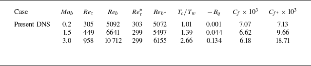


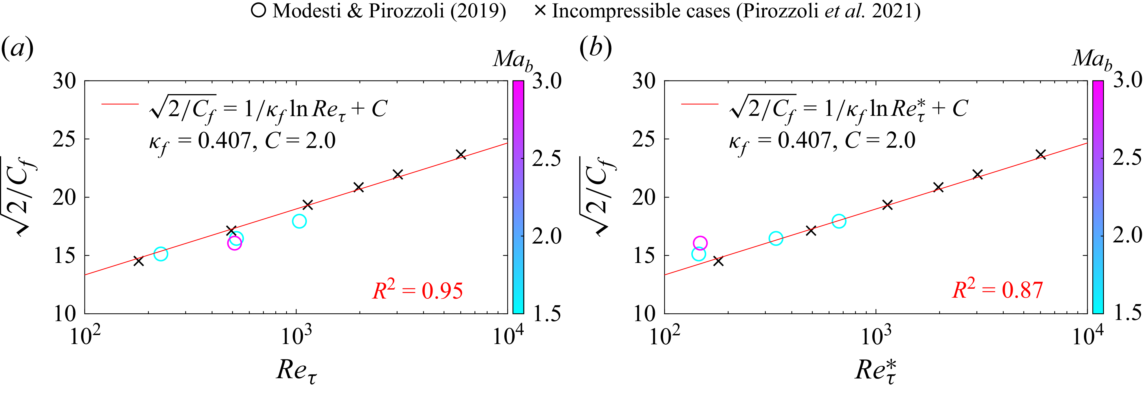


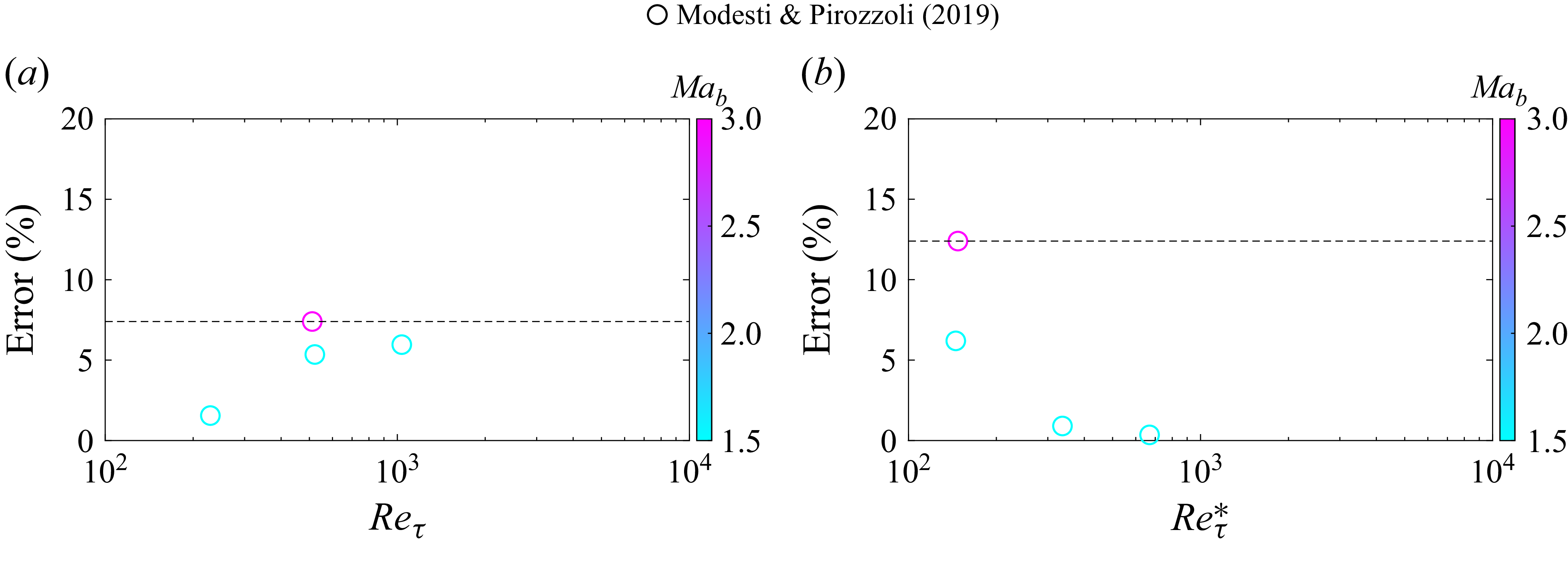


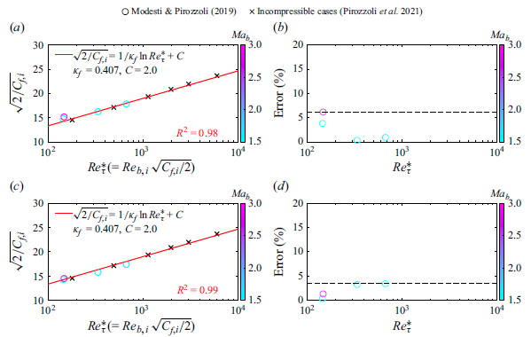


 Open access