


1. Introduction
The International Energy Agency estimated that around 30 % of the energy consumption worldwide is used for transportation (International Energy Agency 2020), with 15 % of this energy spent near the boundaries of the vehicle (Jiménez Reference Jiménez2013). Therefore, a deeper understanding of fluid mechanics and turbulence will have strong implications in fuel consumption, cost savings and reducing carbon dioxide emissions worldwide (Kim Reference Kim2011). Knowing the mechanisms that turbulence uses for transporting energy and generating friction drag is a crucial point for creating new control strategies to face the environmental challenges worldwide (Marusic et al. Reference Marusic, Chandran, Rouhi, Fu, Wine, Holloway, Chung and Smits2021). However, turbulent flows are described by the Navier–Stokes equations (Navier Reference Navier1827; Stokes Reference Stokes2009), a set of partial differential equations whose analytical solution has not been found for a general case of application. Additionally, energy is transported through different scales, from the largest to the smallest ones, until it is dissipated (Kolmogorov Reference Kolmogorov1941), and in the opposite direction (Cardesa, Vela-Martín & Jiménez Reference Cardesa, Vela-Martín and Jiménez2017), requiring costly and large simulations (Hoyas et al. Reference Hoyas, Oberlack, vila, Francisco, Stefanie and Laux2022; Osawa & Jiménez Reference Osawa and Jiménez2024) or experimental tests (Taylor Reference Taylor1938; Kline et al. Reference Kline, Reynolds, Schraub and Runstadler1967; Townsend Reference Townsend1976; Deshpande et al. Reference Deshpande, Van Den, Aron, Ricardo and Marusic2023).
The chaotic behaviour of turbulent flows does not allow extrapolating the instantaneous deterministic predictions of a certain simulation or experimental test to a real-world application. One possibility to overcome this limitation is the use of non-intrusive sensing to reconstruct the flow from external sensors. Non-intrusive techniques have been widely used for experimental tests in fluid dynamics as they do not require placing any sensor inside the rig. The most common techniques involve the use of laser and optical techniques, such as laser-Doppler velocimetry (George & Lumley Reference George and Lumley1973) or particle image velocimetry (Adrian & Westerweel Reference Adrian and Westerweel2011). However, for real-world applications, these techniques are not suitable as the sensing equipment cannot be installed in the device itself. Thus, new methodologies based, for example, on deep learning (LeCun, Bengio & Hinton Reference LeCun, Bengio and Hinton2015) are required to reconstruct the flows from wall measurements (Cuéllar et al. Reference Cuéllar, Güemes, Ianiro, Flores, Vinuesa and Discetti2024a ).
In the last decades, machine learning (ML) has been widely used as a result of the large amounts of available data (Chui et al. Reference Chui, Manyika, Miremadi, Henke, Chung, Nel and Malhotra2018) and the improvement in computational power (Al-Jarrah et al. Reference Al-Jarrah, Yoo, Muhaidat, Karagiannidis and Taha2015). Fluid dynamics is not exempt from this trend, as ML has provided novel possibilities for the analysis of flows. Here, ML models have been used to improve the results of numerical simulations (Vinuesa & Brunton Reference Vinuesa and Brunton2022) and experimental results (Vinuesa, Brunton & McKeon Reference Vinuesa, Brunton and McKeon2023): modelling turbulence (Wang, Wu & Xiao Reference Wang, Wu and Xiao2017; Beck, Flad & Munz Reference Beck, Flad and Munz2019), accelerating the simulations (Bar-Sinai et al. Reference Bar-Sinai, Hoyer, Hickey and Brenner2019; Li et al. Reference Li, Kovachki, Azizzadenesheli, Liu, Bhattacharya, Stuart and Anandkumar2020; Kochkov et al. Reference Kochkov, Smith, Alieva, Wang, Brenner and Hoyer2021; Marino et al. Reference Marino, Juanicotena, Errasti, Mayoral, Manrique de Lara, Vinuesa and Ferrer2024), creating reduced-order models (Kaiser et al. Reference Kaiser, Noack, Cordier, Spohn, Segond, Abel, Daviller, Östh, Krajnović and Niven2014; Lee & Carlberg Reference Lee and Carlberg2020), improving experimental techniques (Rabault, Kolaas & Jensen Reference Rabault, Kolaas and Jensen2017), controlling (Kim et al. Reference Kim, Kim, Song and You2024) and reconstructing flows (Yousif et al. Reference Yousif, Yu, Hoyas, Vinuesa and Lim2023). Related to the flow reconstruction, ML has also been applied to non-intrusive sensing (Lee et al. Reference Lee, Kim, Babcock and Goodman1997; Iñigo et al. Reference Iñigo, Sipp and Schmid2014; Kim & Lee Reference Kim and Lee2020). In these works, wall measurements are used to predict the flow evolution. For instance, Guastoni et al. (Reference Guastoni, Güemes, Ianiro, Discetti, Schlatter, Azizpour and Vinuesa2021) estimated the velocity at a certain wall-normal distance inside a turbulent open channel through a deep-learning model. However, in all these works ML is used as a black-box model. The accuracy of the predictions and the statistics of the reproduced flow are analysed, but the relationships between the inputs and the outputs are not explored. Therefore, a deeper analysis is required to understand the most influential regions for the prediction, if those regions form clusters, and the physical properties of those structures.
Explaining deep-learning models is crucial for understanding the physics of the predicted flow. Additive-feature-attribution methods propose a simplified linear model to understand the relationships between inputs and outputs for a general nonlinear model, capturing the nonlinear interactions between the input features (Cremades, Hoyas & Vinuesa Reference Cremades, Hoyas and Vinuesa2025). These methods are based on the Shapley values (Shapley Reference Shapley1953) and adapted to the architecture of the deep-learning models (Lundberg & Lee Reference Lundberg and Lee2017). Some researchers such as He et al. (Reference He, Tan, Rigas and Vahdati2022), McConkey, Yee & Lien (Reference McConkey, Yee and Lien2022) and Sudharsun & Warrior (Reference Sudharsun and Warrior2023) have applied the additive-feature-attribution methods to understand the effect of the flow parameters in the prediction of the eddy viscosity used in Reynolds averaged Navier–Stokes turbulence modelling (Boussinesq Reference Boussinesq1903). Others, such as Lellep et al. (Reference Lellep, Prexl, Eckhardt and Linkmann2022) or Cremades et al. (Reference Cremades2024a ) have used them to explain the evolution of turbulent flows, understanding, among other phenomena, the implications of the turbulent structures in wall-shear stress (Hoyas et al. Reference Hoyas, Benedikt, Cremades and Vinuesa2025). Applying this methodology to the non-intrusive sensing problem provides new insight into the patterns predicted by the deep-learning model. A proper understanding of them is essential for real-world applications in which the number of sensors is limited and they need to be located optimally.
This work extends the non-intrusive sensing proposed by Guastoni et al. (Reference Guastoni, Güemes, Ianiro, Discetti, Schlatter, Azizpour and Vinuesa2021). The importance of the measured wall pressure and shear stress for the prediction of the velocity fluctuations at a certain wall distance is evaluated. The impact of each input grid point on the model is calculated by applying an additive-feature-attribution method known as deep SHAP (deep Shapley additive explanations) (Lundberg & Lee Reference Lundberg and Lee2017). Then, the grid points are ranked according to their importance for the reconstruction of the flow. Finally, the domain is segmented and the physical properties of the generated coalitions are analysed.
The manuscript is structured as follows. First, the methodology of the feature attribution methods used for the analysis is presented. The workflow is illustrated, and the underlying mathematical framework for the calculations is thoroughly detailed. Then, the results of the explainable methods are discussed. The statistical distribution of each grid point’s importance and its respective wall stress is presented. The connection between the input values and their score in the prediction is unveiled and the sensitivity of the model to each input grid point is evaluated. The domain is segmented into similar-importance coalitions whose properties are calculated and discussed. Finally, the results are summarized, and the main conclusions of the work are presented.
2. Methods
The present work evaluates the importance of the wall pressure and wall-shear stress in a turbulent open-channel at a friction Reynolds number
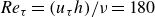 $ \textit{Re}_\tau = (u_\tau h)/\nu = 180$
to predict the velocity fluctuations at a certain wall-normal distance,
$ \textit{Re}_\tau = (u_\tau h)/\nu = 180$
to predict the velocity fluctuations at a certain wall-normal distance,
 $y^+=(u_\tau y)/\nu =15$
. The friction velocity,
$y^+=(u_\tau y)/\nu =15$
. The friction velocity,
 $u_\tau =\sqrt {\tau _w/\rho }$
, is defined based on the shear stress on the wall,
$u_\tau =\sqrt {\tau _w/\rho }$
, is defined based on the shear stress on the wall,
 $\tau _w$
, and the fluid density,
$\tau _w$
, and the fluid density,
 $\rho$
, while
$\rho$
, while
 $\nu$
is the fluid kinematic viscosity. Note that the wall-unit magnitudes are represented by the superscript
$\nu$
is the fluid kinematic viscosity. Note that the wall-unit magnitudes are represented by the superscript
 $^+$
, the averaged value of a variable
$^+$
, the averaged value of a variable
 $x$
by
$x$
by
 $\overline {x}$
, and its standard deviation by
$\overline {x}$
, and its standard deviation by
 $\sigma _x$
. Finally, the standardized values are calculated as
$\sigma _x$
. Finally, the standardized values are calculated as
 $\widetilde {\xi }=(\xi -\overline {\xi })/\sigma _\xi$
.
$\widetilde {\xi }=(\xi -\overline {\xi })/\sigma _\xi$
.
This work modifies the original deep-learning model of Guastoni et al. (Reference Guastoni, Güemes, Ianiro, Discetti, Schlatter, Azizpour and Vinuesa2021) to calculate the importance of the input grid points in the output prediction. The original model predicts the velocity fluctuations from the wall pressure and shear stress using a convolutional neural network (CNN) (LeCun et al. Reference LeCun, Boser, Denker, Henderson, Howard, Hubbard and Jackel1989), exploiting its ability to extract information and local correlation in images or volumes (Murata, Fukami & Fukagata Reference Murata, Fukami and Fukagata2020; Morimoto et al. Reference Morimoto, Fukami, Zhang, Nair and Fukagata2021). Then, to compute the SHAP values, the output of the deep-learning model needs to be reduced to a single scalar that quantifies the accuracy of the predictions. To quantify the accuracy of the CNN, an extra layer is included in the model to calculate the mean squared error (MSE) between the prediction of the original model and the ground truth of each velocity fluctuation. The SHAP values are calculated following two stages, prediction of the velocity and evaluation of the errors, which are summarized in figure 1.
Workflow of the methodology. The figure shows the model used for calculating the SHAP values. This model comprises two stages. The first stage corresponds to the prediction of the velocity fluctuation (yellow boxes) at a wall distance
 $y^+=15$
from the wall measurements (green boxes). The workflow of the velocity prediction is presented with the black arrows. Then, the SHAP values (light green boxes) are calculated using a deep-SHAP explainer. First, the zero-fluctuation fields, mean value of the input or non-informative fields are selected (blue boxes), and then, the output of the model is compared with the ground truth (green boxes) through the MSE.
$y^+=15$
from the wall measurements (green boxes). The workflow of the velocity prediction is presented with the black arrows. Then, the SHAP values (light green boxes) are calculated using a deep-SHAP explainer. First, the zero-fluctuation fields, mean value of the input or non-informative fields are selected (blue boxes), and then, the output of the model is compared with the ground truth (green boxes) through the MSE.

The CNN is trained using the wall pressure
 $p_w$
, and the wall-shear stress in the streamwise and the spanwise directions
$p_w$
, and the wall-shear stress in the streamwise and the spanwise directions
 $\tau _{wx}$
and
$\tau _{wx}$
and
 $\tau _{wz}$
. The model is then used to predict the velocity fluctuations in the streamwise,
$\tau _{wz}$
. The model is then used to predict the velocity fluctuations in the streamwise,
 $u$
, wall-normal,
$u$
, wall-normal,
 $v$
, and spanwise,
$v$
, and spanwise,
 $w$
directions for each grid point in the streamwise direction
$w$
directions for each grid point in the streamwise direction
 $x$
and spanwise direction
$x$
and spanwise direction
 $z$
of a wall-parallel plane. The input and output fields have
$z$
of a wall-parallel plane. The input and output fields have
 $192\times 192$
grid points. A
$192\times 192$
grid points. A
 $15$
grid-point periodic padding is added to the input fields to avoid boundary inaccuracies. As reported by Guastoni et al. (Reference Guastoni, Güemes, Ianiro, Discetti, Schlatter, Azizpour and Vinuesa2021), the network is trained to obtain a reconstruction error lower than 1 %.
$15$
grid-point periodic padding is added to the input fields to avoid boundary inaccuracies. As reported by Guastoni et al. (Reference Guastoni, Güemes, Ianiro, Discetti, Schlatter, Azizpour and Vinuesa2021), the network is trained to obtain a reconstruction error lower than 1 %.
Then, the deep-SHAP algorithm (Lundberg & Lee Reference Lundberg and Lee2017) is used for evaluating the importance of each wall grid point for a total of 1000 fields, corresponding to approximately 5000 viscous time units and approximately 28 eddy turnover times. Due to the complexity of the deep-learning model, sketched in figure 1, the relationships between the inputs and the outputs cannot be understood by analysing the model itself. According to Lundberg & Lee (Reference Lundberg and Lee2017), the most interpretable models are those composed of linear relationships. A clear example of this idea can be understood in the second Newton’s law where the importance of the acceleration for the calculation of the force is interpretable:
 $F=ma$
, where
$F=ma$
, where
 $F$
is the force,
$F$
is the force,
 $m$
the mass and
$m$
the mass and
 $a$
the acceleration. For this reason, a simplified or explainable equivalent model, linear model,
$a$
the acceleration. For this reason, a simplified or explainable equivalent model, linear model,
 $g$
, needs to be calculated. The additive-feature-attribution methods SHAP values are based on this explainable model, as follows, to exploit the explainability potential of the linear models:
$g$
, needs to be calculated. The additive-feature-attribution methods SHAP values are based on this explainable model, as follows, to exploit the explainability potential of the linear models:
 \begin{align} g(q) = \phi _0+\sum _{i=1}^{N}\phi _i q'_i.\end{align}
The additive-feature-attribution methods approximate the original function
 $f$
locally by calculating the marginal contribution to the output of including each input feature in the model. In other words, they reduce the original model
$f$
locally by calculating the marginal contribution to the output of including each input feature in the model. In other words, they reduce the original model
 $f$
to the approximate model
$f$
to the approximate model
 $g$
presented in (2.1). This approximate function is a linear summation of the SHAP values,
$g$
presented in (2.1). This approximate function is a linear summation of the SHAP values,
 $\phi _i$
, for the input feature
$\phi _i$
, for the input feature
 $q'_i$
, which is a Boolean value equal to
$q'_i$
, which is a Boolean value equal to
 $1$
if the feature is present and
$1$
if the feature is present and
 $0$
if it is absent, with
$0$
if it is absent, with
 $N$
being the total number of input features. The value
$N$
being the total number of input features. The value
 $\phi _0$
equals the function
$\phi _0$
equals the function
 $g$
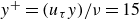
when all the features are absent, in other words, when the non-informative input is used, in the case of the turbulent flow, a field in which there is no information transfer, or in other words, there are no fluctuations. These additive-feature-attribution methods must satisfy three axioms: local accuracy, missingness and consistency (Lundberg & Lee Reference Lundberg and Lee2017). The only possible solution that satisfies all of them at the same time is the Shapley values (Shapley Reference Shapley1953):
$g$
when all the features are absent, in other words, when the non-informative input is used, in the case of the turbulent flow, a field in which there is no information transfer, or in other words, there are no fluctuations. These additive-feature-attribution methods must satisfy three axioms: local accuracy, missingness and consistency (Lundberg & Lee Reference Lundberg and Lee2017). The only possible solution that satisfies all of them at the same time is the Shapley values (Shapley Reference Shapley1953):
 \begin{align} \phi _{i} = \sum _{S\subseteq F\backslash \left \{i\right \}}\frac {\left |S\right |!\left (N-\left |S\right |-1\right )!}{N!}\big [f (S\cup i)-f(S)\big ] \text{.} \end{align}
Here the Shapley values
 $\phi _i$
of the feature
$\phi _i$
of the feature
 $i$
are calculated as a weighted average of the error in the output model of a certain subset
$i$
are calculated as a weighted average of the error in the output model of a certain subset
 $S$
, before and after adding the feature
$S$
, before and after adding the feature
 $i$
:
$i$
:
 $[f(S\cup i)-f(S)]$
. The subset is taken from the total set
$[f(S\cup i)-f(S)]$
. The subset is taken from the total set
 $F$
that does not include the feature
$F$
that does not include the feature
 $i$
. The error is averaged by weighting its value with the probability of the subset
$i$
. The error is averaged by weighting its value with the probability of the subset
 $S$
to be taken before the feature
$S$
to be taken before the feature
 $i$
:
$i$
:
 $(|S|!(N-|S|-1)!)/(N!)$
. The parameter
$(|S|!(N-|S|-1)!)/(N!)$
. The parameter
 $|S|$
represents the number of not null features in the subset
$|S|$
represents the number of not null features in the subset
 $S$
and
$S$
and
 $N$
is the total number of subsets. The computation of the Shapley value scales exponentially with the number of input features,
$N$
is the total number of subsets. The computation of the Shapley value scales exponentially with the number of input features,
 $2^N$
, making its calculation extremely expensive for deep learning models (Jia et al. Reference Jia, Dao, Wang, Hubis, Hynes, Gürel, Li, Zhang, Song and Spanos2019). In order to clarify the Shapley values calculation the reader is referred to figure 2.
$2^N$
, making its calculation extremely expensive for deep learning models (Jia et al. Reference Jia, Dao, Wang, Hubis, Hynes, Gürel, Li, Zhang, Song and Spanos2019). In order to clarify the Shapley values calculation the reader is referred to figure 2.
Visualization of the Shapley value calculations. The figure shows the calculation of the SHAP value of
 $x_2$
. A total set of features
$x_2$
. A total set of features
 $F$
composed of three features
$F$
composed of three features
 $x_1$
,
$x_1$
,
 $x_2$
and
$x_2$
and
 $x_3$
is stated. From this set, a subset
$x_3$
is stated. From this set, a subset
 $S$
not including the feature
$S$
not including the feature
 $x_2$
is defined. The probability of the coalition
$x_2$
is defined. The probability of the coalition
 $S$
to happen and the calculation of the output for
$S$
to happen and the calculation of the output for
 $S$
and
$S$
and
 $S \cup i$
is visualized.
$S \cup i$
is visualized.

To reduce the computational requirements of the Shapley values, they can be approximated by applying the knowledge of the model architecture. This work uses the deep-SHAP methodology, a combination of the Deep LIFT (learning important features) (Ribeiro, Singh & Guestrin Reference Ribeiro, Singh and Guestrin2016) and the Shapley values, for computing the importance of the input features in the output predictions. The SHAP values are calculated assuming independent features and a linear model. Although adjacent grid points in a flow are not independent for any resolution of the grid, this hypothesis had to be assumed to contain the computational cost of the SHAP-value computation. The dependency has been included in the calculation of previous works, such as Giudici & Raffinetti (Reference Giudici and Raffinetti2021), who included dependency for the calculation of Shapley values. However, the cost of the calculation grows exponentially with the number of features, becoming unfeasible for the number of grid points of a turbulent flow measurement, and requiring the use of simplified methodologies such as deep SHAP which rely on independence of features. In the case of a strong dependence between features, the violation of the assumption would result in a deviation of the importance of these features (Song, Nelson & Staum Reference Song, Nelson and Staum2016). In these circumstances, the importance of a grid point could flow to the adjacent ones (dependent grid points of the turbulent flow), producing noise in the solution. This was addressed in a previous work (Cremades et al. Reference Cremades, Hoyas and Vinuesa2024b
) where it was overcome by exploiting the periodic conditions of the domain and averaging the results, smothering the noise as the dependence affects the flow differently for every movement, exemplified in figure 3. Nevertheless, as will be observed later, the absolute value of the SHAP values used for the analysis do not present noise, therefore the previous hypothesis could be assumed as it is not producing relevant deviation in the results and including the dependency is not feasible. Deep LIFT calculates the variation in the output
 $\Delta o$
as the summation of the attributions,
$\Delta o$
as the summation of the attributions,
 $\Delta o = \sum _{i=1}^{n} C_{\Delta \xi _{i},\Delta o}$
, of the
$\Delta o = \sum _{i=1}^{n} C_{\Delta \xi _{i},\Delta o}$
, of the
 $n$
input feature
$n$
input feature
 $\xi _i$
concerning its reference value
$\xi _i$
concerning its reference value
 $\xi _{ir}$
,
$\xi _{ir}$
,
 $\Delta \xi _{i} = \xi _i-\xi _{ir}$
. The attributions of the Deep-LIFT method,
$\Delta \xi _{i} = \xi _i-\xi _{ir}$
. The attributions of the Deep-LIFT method,
 $C_{\Delta \xi _{i},\Delta o}$
, are equivalent to the SHAP values
$C_{\Delta \xi _{i},\Delta o}$
, are equivalent to the SHAP values
 $\phi _{i}$
and
$\phi _{i}$
and
 $f(\xi _{r})$
equals
$f(\xi _{r})$
equals
 $\phi _0$
. In the deep-SHAP methodology, the SHAP values of the smaller components (layers of the model) are calculated by approximating the model linearly,
$\phi _0$
. In the deep-SHAP methodology, the SHAP values of the smaller components (layers of the model) are calculated by approximating the model linearly,
 \begin{align} \phi _{i}\left (f_{j},\xi \right ) \approx m_{\xi _{i},f_{j}}\left (\xi _{i}-\mathbb{E}\left [\xi _{i}\right ]\right ), \end{align}
Noise visualization in the solution generated by dependent features. Panel (a) represents the initial SHAP values result, while panel (b) shows how the noise could be diluted by exploiting the periodic conditions and averaging the solutions. The results were taken from the prelaminar analysis of a previous work (Cremades et al. Reference Cremades, Hoyas and Vinuesa2024b ).

where
 $f_{\kern-1.5pt j}$
refers to the component
$f_{\kern-1.5pt j}$
refers to the component
 $j$
of the model
$j$
of the model
 $f$
,
$f$
,
 $m_{\xi _{i},f_{j}}$
is the coefficient or attribution of the feature
$m_{\xi _{i},f_{j}}$
is the coefficient or attribution of the feature
 $\xi _i$
in the calculation of the output of the component
$\xi _i$
in the calculation of the output of the component
 $j$
of the model
$j$
of the model
 $f$
and
$f$
and
 $\mathbb{E}[\xi _{i}]$
the expected value of the feature
$\mathbb{E}[\xi _{i}]$
the expected value of the feature
 $\xi _i$
. Then, these local SHAP values are recursively passed backward in the network using the chain rule to obtain the SHAP values of the complete model (Lundberg & Lee Reference Lundberg and Lee2017; Cremades et al. Reference Cremades, Hoyas and Vinuesa2025). The process is started taking the difference in the output from the original input and the reference input. In deep LIFT, the SHAP values of a layer are calculated as the difference of the outputs of the layer
$\xi _i$
. Then, these local SHAP values are recursively passed backward in the network using the chain rule to obtain the SHAP values of the complete model (Lundberg & Lee Reference Lundberg and Lee2017; Cremades et al. Reference Cremades, Hoyas and Vinuesa2025). The process is started taking the difference in the output from the original input and the reference input. In deep LIFT, the SHAP values of a layer are calculated as the difference of the outputs of the layer
 $j$
calculated from the input,
$j$
calculated from the input,
 $\xi$
, and the reference or expected input,
$\xi$
, and the reference or expected input,
 $\mathbb{E}[\xi ]$
:
$\mathbb{E}[\xi ]$
:
 \begin{align} \phi _i = \left (f_{\kern-1.5pt j}(\xi)-f_{\kern-1.5pt j}\left (\mathbb{E} [\xi]\right )\right )_i\text{.} \end{align}
Concerning the expression of (2.3), a coefficient
 $m_{\xi _i,f_o}=1$
is employed for the output layer,
$m_{\xi _i,f_o}=1$
is employed for the output layer,
 $o$
. Then, the information is backpropagated through the model obtaining the coefficients
$o$
. Then, the information is backpropagated through the model obtaining the coefficients
 $m_{\xi _i,f_{\kern-1.5pt j}}$
through the calculation of the internal SHAP values. This complete cycle is illustrated in figure 4 where the pink flow represents the backpropagation of the information to obtain the coefficients
$m_{\xi _i,f_{\kern-1.5pt j}}$
through the calculation of the internal SHAP values. This complete cycle is illustrated in figure 4 where the pink flow represents the backpropagation of the information to obtain the coefficients
 $m_{\xi _i,f_{\kern-1.5pt j}}$
and the black flow represents the calculation of the SHAP values at each step.
$m_{\xi _i,f_{\kern-1.5pt j}}$
and the black flow represents the calculation of the SHAP values at each step.
Sketch of the deep-SHAP algorithm. First the information is backpropagated to calculate the coefficients
 $m_{\xi _i,f_{\kern-1.5pt j}}$
(pink flow). Then, these coefficients are used for the calculation of the SHAP values in all the internal elements of the network (black flow).
$m_{\xi _i,f_{\kern-1.5pt j}}$
(pink flow). Then, these coefficients are used for the calculation of the SHAP values in all the internal elements of the network (black flow).

3. Results
An importance field, i.e. the SHAP values for all the input grid points, is calculated by correlating each input wall stress (streamwise shear stress, spanwise shear stress and pressure) with its importance in the calculation of the velocity fluctuation in one direction (streamwise, wall-normal, spanwise) at a wall-normal distance
 $y^+=15$
. The SHAP values are calculated by comparing the input fields with a non-informative reference, the mean value of the wall-shear stress and pressure
$y^+=15$
. The SHAP values are calculated by comparing the input fields with a non-informative reference, the mean value of the wall-shear stress and pressure
 $i$
. The larger the magnitude of the SHAP values used for this purpose, the more sensitive the model output is to any change in the input feature. Figure 5 shows the instantaneous normalized SHAP values,
$i$
. The larger the magnitude of the SHAP values used for this purpose, the more sensitive the model output is to any change in the input feature. Figure 5 shows the instantaneous normalized SHAP values,
 \begin{align} \hat {\phi }_{u,p}\left (x_{\textit{ij}},z_{\textit{ij}}\right )=\frac {3 N_x N_z\left \vert \phi _{u,p}\left (x_{\textit{ij}},z_{\textit{ij}}\right )\right \vert }{\sum _{i=1}^{N_x}\sum _{j=1}^{N_z}\sum _{p=1}^{3}\left |\phi _{u,p}\left (x_{\textit{ij}},z_{\textit{ij}}\right )\right |}\text{,} \end{align}
where the subindexes
 $u$
,
$u$
,
 $p$
,
$p$
,
 $i$
and
$i$
and
 $j$
indicate the velocity component (output of the model), wall stress (input of the model), streamwise position index and spanwise position index, respectively. Here
$j$
indicate the velocity component (output of the model), wall stress (input of the model), streamwise position index and spanwise position index, respectively. Here
 $N_x$
is the maximum number of grid points in the streamwise direction and
$N_x$
is the maximum number of grid points in the streamwise direction and
 $N_z$
the maximum number of grid points in the spanwise direction. Therefore, these images visualize whether and how the importance scores correlate with the input.
$N_z$
the maximum number of grid points in the spanwise direction. Therefore, these images visualize whether and how the importance scores correlate with the input.
Instantaneous visualization of the wall measurements of the open channel (streamwise wall-shear stress
 $\tau _{wx}$
, spanwise wall-shear stress
$\tau _{wx}$
, spanwise wall-shear stress
 $\tau _{wz}$
and wall-normal pressure
$\tau _{wz}$
and wall-normal pressure
 $p_w$
) and their corresponding SHAP values for the predictions of the velocity fluctuations (
$p_w$
) and their corresponding SHAP values for the predictions of the velocity fluctuations (
 $u$
,
$u$
,
 $v$
and
$v$
and
 $w$
). Linear colourmaps have been used in the figure.
$w$
). Linear colourmaps have been used in the figure.

Figure 5 shows the instantaneous standarized wall pressure and shear stress,
 \begin{align} \widetilde {p}_{w}=\frac {p_{w}-\overline {p_{w}}}{\sigma _{p_{w}}},\quad \widetilde {\tau }_{wx}=\frac {\tau _{wx}-\overline {\tau _{wx}}}{\sigma _{\tau _{wx}}}\quad\text{ and }\quad \widetilde {\tau }_{wz}=\frac {\tau _{wz}-\overline {\tau _{wz}}}{\sigma _{\tau _{wz}}}\text{,} \end{align}
as well as the corresponding SHAP values for predicting the velocity fluctuations at
 $y^+=15$
. The SHAP values detect the high-importance regions of the model, which represent a trajectory of the turbulent flow. Therefore, we can infer that the SHAP values detect the regions of the flow that are most influential for the reconstruction of the fluctuations of the velocity. High-interest regions are those with a high absolute SHAP value. The figure demonstrates that the important regions for the predictions are localized in small clusters of the flow, while most of the grid points exhibit low importance. The visual resemblance between the inputs and their SHAP values might be inferred from the figure. In fact, SHAP values related to the streamwise shear stress at the wall tend to create elongated structures, which are observed more clearly in the prediction of the streamwise velocity due to the strong correlation between both variables (Cuéllar et al. Reference Cremades, Hoyas and Vinuesa2024b
). Similarities between the input and the SHAP values are also observed for the spanwise shear stress and pressure, albeit the high-importance clusters are less elongated than the corresponding streamwise shear stress SHAP clusters. In addition, the figure demonstrates that the model is highly sensitive to the pressure variations as the maximum normalized SHAP value for the pressure is higher than for the shear stress in the prediction of a specific component of the velocity fluctuation.
$y^+=15$
. The SHAP values detect the high-importance regions of the model, which represent a trajectory of the turbulent flow. Therefore, we can infer that the SHAP values detect the regions of the flow that are most influential for the reconstruction of the fluctuations of the velocity. High-interest regions are those with a high absolute SHAP value. The figure demonstrates that the important regions for the predictions are localized in small clusters of the flow, while most of the grid points exhibit low importance. The visual resemblance between the inputs and their SHAP values might be inferred from the figure. In fact, SHAP values related to the streamwise shear stress at the wall tend to create elongated structures, which are observed more clearly in the prediction of the streamwise velocity due to the strong correlation between both variables (Cuéllar et al. Reference Cremades, Hoyas and Vinuesa2024b
). Similarities between the input and the SHAP values are also observed for the spanwise shear stress and pressure, albeit the high-importance clusters are less elongated than the corresponding streamwise shear stress SHAP clusters. In addition, the figure demonstrates that the model is highly sensitive to the pressure variations as the maximum normalized SHAP value for the pressure is higher than for the shear stress in the prediction of a specific component of the velocity fluctuation.
From a statistical point of view, figure 6(a) shows the joint histogram distribution between standardized streamwise wall-shear stress and its importance scores
 $\phi _{u,\tau _{wx}}$
to predict the streamwise velocity fluctuation
$\phi _{u,\tau _{wx}}$
to predict the streamwise velocity fluctuation
 $u$
. Note that the figure accounts for the correlation of every grid point for a total time
$u$
. Note that the figure accounts for the correlation of every grid point for a total time
 $\Delta t^+\approx 5000$
. The figure shows that a wide range of points are located near the mean value of the input,
$\Delta t^+\approx 5000$
. The figure shows that a wide range of points are located near the mean value of the input,
 $\widetilde {\tau }_{wx}=0$
. However, these grid points are related to low-importance scores. The higher importance is located from one to two standard deviations, while the domain areas containing peak values of the streamwise wall shear stress are less likely and do not present a high-importance content. This fact provides an important idea: the SHAP values do not directly correlate with wall shear stress values, similarly as observed by Cremades et al. (Reference Cremades2024a
) for the evaluation of the intense Reynolds stress structures (Lozano-Durán et al. Reference Lozano-Durán, Flores and Jiménez2012; Jiménez Reference Jiménez2018).
$\widetilde {\tau }_{wx}=0$
. However, these grid points are related to low-importance scores. The higher importance is located from one to two standard deviations, while the domain areas containing peak values of the streamwise wall shear stress are less likely and do not present a high-importance content. This fact provides an important idea: the SHAP values do not directly correlate with wall shear stress values, similarly as observed by Cremades et al. (Reference Cremades2024a
) for the evaluation of the intense Reynolds stress structures (Lozano-Durán et al. Reference Lozano-Durán, Flores and Jiménez2012; Jiménez Reference Jiménez2018).
Distribution of the SHAP values for the input feature values.Panel (a) shows the distribution of the
 $\tau _{wx}$
input SHAP values for the
$\tau _{wx}$
input SHAP values for the
 $u$
prediction collected over
$u$
prediction collected over
 $\Delta t^+\approx 5000$
. The red line indicates the threshold of the 99th percentile. Panel (b) presents the 99th percentile for all the combination input–output.
$\Delta t^+\approx 5000$
. The red line indicates the threshold of the 99th percentile. Panel (b) presents the 99th percentile for all the combination input–output.

In addition, to easily compare all input–output pairs a threshold line is created. This line (red line in figure 6
a) represents the 99th percentile of the SHAP value. The domain below the line contains 99 % of the input scores for the respective field value. The 99th percentile line is used for comparing the different pairs of input–output combinations, figure 6(b). Regarding the input variables, pressure is the most sensitive parameter for predicting velocity fluctuations in models where both wall pressure and wall-shear stress are available. Although wall-shear stress has been identified as the most influential factor for reconstructing streamwise velocity at this wall-normal distance (Cuéllar et al. Reference Cuéllar, Ianiro and Discetti2024b
), once the model has access to both wall-shear stress and pressure, sudden changes in pressure tend to cause larger errors in the deep-learning model than equivalent changes in wall-shear stress. This is because the three input fields (wall pressure and the two components of wall-shear stress) are used together to reconstruct the flow at a given distance from the wall. Altering the pressure significantly disrupts the learned interaction patterns among these inputs, leading to a greater impact on the model performance. This demonstrates that the estimator is more sensitive to missing or corrupted pressure information. The high correlation between the velocity-fluctuation prediction and the wall pressure detected by the SHAP values is consistent with the results of Ghaemi & Scarano (Reference Ghaemi and Scarano2013), due to the peak of self-similar scaling of coherence presented by Baars, Dacome & Lee (Reference Baars, Dacome and Lee2024) for
 $y^+\approx 15$
and streamwise wavelength
$y^+\approx 15$
and streamwise wavelength
 $\lambda _x\approx 210$
. The high-importance structures, the maximum of the SHAP values, affecting all the velocity components, are located in a range of wall pressure between 1.5 and 2.8 standard deviations.
$\lambda _x\approx 210$
. The high-importance structures, the maximum of the SHAP values, affecting all the velocity components, are located in a range of wall pressure between 1.5 and 2.8 standard deviations.
Regarding the shear stress, both the streamwise and spanwise exhibit similar maximum values for the prediction of the streamwise velocity. Although this idea is non-intuitive, as the streamwise shear could be expected to produce higher effects on the streamwise velocity than the spanwise, the model is trained to predict the velocity based on the combined effect of the wall-pressure and the wall-shear stress. This fact results in higher errors when the correlation between the input variables is broken; for this reason, the pressure becomes the most influential and reduces the effect of the streamwise wall-shear stress. Moreover, the higher SHAP-values for the spanwise and wall-normal velocity are obtained for the negative pressure values. This idea is in agreement with the work of Jeong et al. (Reference Jeong, Hussain, Schoppa and Kim1997), who reported that the negative pressure regions are located below the near-wall coherent structures. In addition, although both shear stresses present similar maximum values, the range in which the high-importance regions are located is much higher for the spanwise than for the streamwise wall-shear stress. The former presents a symmetric distribution of high-importance regions, from 1.15 to 3.5 standard deviations, in both positive and negative values. Concerning the streamwise wall-shear stress, the distribution of high-importance regions is asymmetric, exhibiting a smaller range for the negative velocity, from 1 to 2 standard deviations, than for the positive, from 1 to 4 standard deviations. The asymmetric distribution has previously been pointed out by Lenaers et al. (Reference Lenaers, Li, Brethouwer, Schlatter and Örlü2012), and although the probability of positive wall-shear stress is higher (Vinuesa, Örlü & Schlatter Reference Vinuesa, Örlü and Schlatter2017; Chin et al. Reference Chin, Vinuesa, Örlü, Cardesa, Noorani, Chong and Schlatter2020), the importance associated with the negative values of the shear stress is similar to that of the positive. This idea is connected to the ejection-like structures, i.e. the structures with low streamwise velocity near the wall, that are transporting the energy from the wall to the high-mean velocity regions of the flow. Additionally, note that the higher values of the positive streamwise shear stress that are related to energetic quasistreamwise vortices (Guerrero, Lambert & Chin Reference Guerrero, Lambert and Chin2020) exhibit low SHAP values, which is consistent with the work of Cremades et al. (Reference Cuéllar, Ianiro and Discetti2024b ), which demonstrated the lower importance of the vortices compared with the Q events. The ideas are connected to the near-wall self-sustaining cycle, as the ejection-like regions appear simultaneously to the quasistreamwise vortices which amplify the low-velocity streaks through the lift-up effect (Waleffe Reference Waleffe1997; Schoppa & Hussain Reference Schoppa and Hussain2000; Jiménez & Pinelli Reference Jiménez and Pinelli1999).
Completely different effects are observed in the case of the spanwise velocity. As could be expected, the spanwise velocity is more affected by the spanwise shear, which forces the motion transversely to the main forcing of the channel, than by the streamwise shear, which is expected to force the motion in the same direction as the pressure gradient. Finally, similar trends are observed for the wall-normal velocity, which is mainly affected by the variations on the pressure and then in the spanwise shear stress. Consequently, the spanwise shear stress is more important for the wall-normal and spanwise velocities than for the streamwise velocity.
The distribution of figure 6(b) shows that for all the input–output pairs, the higher importance is not obtained for the most intense input regions. The spatial agreement between the 20 % most important and the 20 % most intense input regions remains below 60 % of their total surface. In addition, the most important regions neither match the intense output locations (intense velocity regions), being the coincidence lower than 45 %. Therefore, those regions affecting the predictions the most have been demonstrated to be strongly related to the model instead of the intense input and output regions. However, a new question is raised: How much does each percentile of importance condition the estimation?
To answer the previous question, a certain fraction containing the highest nth percentile of grid points is removed from the input field and set to their mean value. In other words, the grid points from the input fields are gradually removed according to their importance, evaluating the accuracy of the predictions progressively. The accuracy is evaluated by measuring the MSE of the predicted velocity fluctuations. The evaluation of the MSE as a function of the percentage of top-grid points removed is presented in figure 7. The normalized MSE (
 $\text{MSE}^*$
) of the figure is calculated as follows:
$\text{MSE}^*$
) of the figure is calculated as follows:
 \begin{align} \text{MSE}^*= \frac {1}{3}\left (\frac {\text{MSE}_u}{u^2_{\textit{max}}}+\frac {\text{MSE}_v}{v^2_{\textit{max}}}+\frac {\text{MSE}_w}{w^2_{\textit{max}}}\right )\!. \end{align}
The MSE of velocity fluctuations as a function of the fraction of grid points removed from the input (a) and fraction of grid points of the prediction containing 50 % of the total MSE score for the streamwise velocity fluctuation (b). The fraction of grid-point removal relative to their total number is presented by
 ${n}_{\textit{rm}v}/{n}_{\textit{tot}}$
, and the fraction of grid-point removal for half of the error is
${n}_{\textit{rm}v}/{n}_{\textit{tot}}$
, and the fraction of grid-point removal for half of the error is
 ${n}_{\textit{rm}v}/{n}_{\textit{tot}}|_{50\%{error}}$
.
${n}_{\textit{rm}v}/{n}_{\textit{tot}}|_{50\%{error}}$
.

The results of figure 7(a) correspond to different inputs being modified separately. As expected after the analysis presented in figure 6, the most influential input field is the wall pressure, while wall shear stress in both streamwise and spanwise directions is less important. The results for the pressure show that a fast increase in the error is produced when the initial percentiles of important grid points are removed. A maximum error of the normalized MSE of 50 % of the maximum value of the original squared velocity is obtained when approximately 30 % of the grid points are removed. After this point, the input field becomes non-informative, and therefore the error starts to decrease, until the error generated by removing pressure data is lower than the error of removing wall-shear-stress data. This fact links to the work of Cuéllar et al. (Reference Cuéllar, Güemes, Ianiro, Flores, Vinuesa and Discetti2024a
), who reported that the flow can be reproduced from the wall-shear stress with a lower error, since the corresponding correlation is stronger. However, the peak of self-similar scaling of coherence between wall pressure and streamwise velocity is located for
 $y^+\approx 15$
, explaining the high error when the pressure channel is modified (Baars et al. Reference Baars, Dacome and Lee2024). The decrease is not observed in the case of the wall shear stress due to the high influence of the pressure in the predictions. This effect is produced by the strong correlation between the pressure and shear stress fluctuations. When the pressure fluctuation is affected, its variation results in an increase of error of the model, which is unable to detect the combined patterns of both magnitudes. Figure 6 showed that the maximum importance was obtained for intense values of the standardized wall-pressure and wall-shear stress between
$y^+\approx 15$
, explaining the high error when the pressure channel is modified (Baars et al. Reference Baars, Dacome and Lee2024). The decrease is not observed in the case of the wall shear stress due to the high influence of the pressure in the predictions. This effect is produced by the strong correlation between the pressure and shear stress fluctuations. When the pressure fluctuation is affected, its variation results in an increase of error of the model, which is unable to detect the combined patterns of both magnitudes. Figure 6 showed that the maximum importance was obtained for intense values of the standardized wall-pressure and wall-shear stress between
 $1.5$
and
$1.5$
and
 $2.5$
. As it can be observed in figures 8 and 7, a non-negligible fraction of the intense-shear stress regions,
$2.5$
. As it can be observed in figures 8 and 7, a non-negligible fraction of the intense-shear stress regions,
 $\vert \widetilde {\tau }_{wx}\vert \geqslant 1.5$
and
$\vert \widetilde {\tau }_{wx}\vert \geqslant 1.5$
and
 $\vert \widetilde {\tau }_{wz}\vert \geqslant 1.5$
, correlate with intense wall-pressure regions,
$\vert \widetilde {\tau }_{wz}\vert \geqslant 1.5$
, correlate with intense wall-pressure regions,
 $\vert \widetilde {p}_{w}\vert \geqslant 1.5$
. For this reason, although the streamwise velocity fluctuation at a wall-normal distance
$\vert \widetilde {p}_{w}\vert \geqslant 1.5$
. For this reason, although the streamwise velocity fluctuation at a wall-normal distance
 $y^+=15$
correlates mostly with the streamwise shear stress, modifying the pressure associated with this region modifies the pattern detected by the deep-learning model, increasing the error. However, when the percentage of removed grid points is increased, the pressure field becomes non-informative and the model only relies on the values of the shear stress. The normalized error produced by the streamwise and spanwise shear stress reaches a plateau when approximately 20 % of grid points have been removed and then it remains around 7.5 %. This plateau is produced due to the high influence of the pressure in the prediction of the flow, as when the shear stress becomes non-informative, the model relies on the pressure.
$y^+=15$
correlates mostly with the streamwise shear stress, modifying the pressure associated with this region modifies the pattern detected by the deep-learning model, increasing the error. However, when the percentage of removed grid points is increased, the pressure field becomes non-informative and the model only relies on the values of the shear stress. The normalized error produced by the streamwise and spanwise shear stress reaches a plateau when approximately 20 % of grid points have been removed and then it remains around 7.5 %. This plateau is produced due to the high influence of the pressure in the prediction of the flow, as when the shear stress becomes non-informative, the model relies on the pressure.
Joint probability density function (PDF) of the wall-pressure and wall-shear stress in the streamwise direction (a) and the spanwise direction (b). The black contours highlight the regions of high importance.

The high impact of the top-ranked grid points is presented in figure 9. In the figure, the original wall pressure field is presented (figure 9
a). This field is modified by removing the top 1 % grid points black contours in (figure 9
b) and setting them to their reference value. The bottom images show the original and modified prediction. The figure evidences how a small percentage of grid points, 1 %, modify a much larger region (figure 9
d), which overflows the predictions, generating a velocity value much higher than the original. The analysis of the modified regions of the flow matches the effect of the receptive field. The CNN presented in Guastoni et al. (Reference Guastoni, Güemes, Ianiro, Discetti, Schlatter, Azizpour and Vinuesa2021) has a receptive field of
 $15\times 15$
, meaning that each input value can affect the 15 adjacent values, as can be observed in figure 9(d).
$15\times 15$
, meaning that each input value can affect the 15 adjacent values, as can be observed in figure 9(d).
Then, in figure 7(b), the fraction of grid points of the output contributing to half of the error value is visualized against the fraction of grid points removed from the input. The results show that initially when the first decile of input grid points is removed, half of the total error is concentrated in a small area, below 10 % of the total output. However, as the fraction of the removed input grid points is increased, the error is propagated up to 15 % of the output field in the case of the shear stress and 20 % in the case of the pressure. From this point in advance, half of the error remains concentrated in around 20 % of the output domain. Figure 10 shows the prediction of the model when the whole pressure field is removed from the predictions. The results clearly demonstrate that small modifications of the pressure produce high errors, while skipping the whole field makes the model rely on the wall-shear stress, consequently improving the predictions.
Comparison between original (a,c) and modified (b,d) wall pressure with top 1 % absolute SHAP values removed from the predictions of the streamwise velocity. Panels (a) and (b) show the wall pressure field and panels (c) and (d) the predicted streamwise velocity. The black dots in (b) indicate the input grid points replaced by the non-informative background value, while the modified streamwise velocity prediction is capped at the original prediction maximum values to indicate the changes in prediction.

Comparison between original (a,c) and modified (b,d) wall pressure removed from the predictions of the streamwise velocity. Panels (a) and (b) show the wall pressure field and panels (c) and (d) image the predicted streamwise velocity. The modified streamwise velocity prediction is capped at the original prediction maximum values to indicate the changes in prediction.

To understand the input structures that are conditioning the prediction of the model, the domain is segmented in deciles. Then, the grid points corresponding to each decile segmentation are joined into structures, filtering those with an area in viscous units smaller than
 $S^+ = 30^2$
(Lozano-Durán et al. Reference Lozano-Durán, Flores and Jiménez2012). The probability of the filtered structures belonging to each importance decile is calculated over 1000 snapshots,
$S^+ = 30^2$
(Lozano-Durán et al. Reference Lozano-Durán, Flores and Jiménez2012). The probability of the filtered structures belonging to each importance decile is calculated over 1000 snapshots,
 $\Delta t^+\approx 5000$
, as described in figure 11(a). The figure evidences that only the structures of the first (red) and the last deciles (blue) are significant, the rest are too small to pass the filter as they are scattered around and are not big enough to form clusters. Finally, the averaged physical properties of the formed clusters are analysed against their impact on the prediction to understand the common properties of the high and low-importance regions.
$\Delta t^+\approx 5000$
, as described in figure 11(a). The figure evidences that only the structures of the first (red) and the last deciles (blue) are significant, the rest are too small to pass the filter as they are scattered around and are not big enough to form clusters. Finally, the averaged physical properties of the formed clusters are analysed against their impact on the prediction to understand the common properties of the high and low-importance regions.
Probability of the most important clusters for predicting the streamwise velocity from the wall pressure. Probability of the structures belonging to each percentile of importance (a), and joint probability of their averaged physical properties and importance: pressure (b), streamwise velocity (c), aspect ratio (d), streamwise length (e) and spanwise width (f).

The analysis of the wall pressure averaged over the area of the most important and the least important deciles of structures are presented in figure 11(b). As previously discussed, pressure is the input variable with a higher impact on the predictions at a wall distance
 $y^+=15$
. The figure shows symmetrical distributions for the high-impact structures (red), which are distributed from one to two standard deviations from the mean pressure, showing equivalent impact in the solution for positive and negative fluctuations of the pressure. On the other hand, a low-importance region is detected for averaged pressures. Then, the values of the averaged streamwise velocity predicted over this region are analysed. The results evidenced that the high-importance regions on the wall are mostly located below low streamwise velocity areas (L), low-velocity streaks, or ejection-like regions in contrast to the high-velocity or sweep-like regions (H). On the other hand, the lower-importance regions are slightly skewed to positive-velocity values. This idea is consistent with the results of Cremades et al. (Reference Cremades2024a
), in which the ejection-like regions were demonstrated to be the most influential for the reconstruction of the future flow at low friction Reynolds numbers. In addition, note the small values of the deviation from the mean of the averaged velocities along the structure area. This fact shows that the high-importance regions contain high and low-velocity areas and also connect with the results of Cremades et al. (Reference Cremades2024a
) which evidenced that the most important areas are not those with the highest Reynolds stress. Concerning the shape and size of the structures, the high-intensity structures are slightly elongated in the streamwise direction. This elongation is a result of the anisotropy of the turbulence in the channel. The flow forces the structures to move in the streamwise direction creating elongated patterns. In addition, the size of the structures, in both streamwise and spanwise directions, is evaluated to provide an objective criterion for placing the sensors. Most of the important structures measure around
$y^+=15$
. The figure shows symmetrical distributions for the high-impact structures (red), which are distributed from one to two standard deviations from the mean pressure, showing equivalent impact in the solution for positive and negative fluctuations of the pressure. On the other hand, a low-importance region is detected for averaged pressures. Then, the values of the averaged streamwise velocity predicted over this region are analysed. The results evidenced that the high-importance regions on the wall are mostly located below low streamwise velocity areas (L), low-velocity streaks, or ejection-like regions in contrast to the high-velocity or sweep-like regions (H). On the other hand, the lower-importance regions are slightly skewed to positive-velocity values. This idea is consistent with the results of Cremades et al. (Reference Cremades2024a
), in which the ejection-like regions were demonstrated to be the most influential for the reconstruction of the future flow at low friction Reynolds numbers. In addition, note the small values of the deviation from the mean of the averaged velocities along the structure area. This fact shows that the high-importance regions contain high and low-velocity areas and also connect with the results of Cremades et al. (Reference Cremades2024a
) which evidenced that the most important areas are not those with the highest Reynolds stress. Concerning the shape and size of the structures, the high-intensity structures are slightly elongated in the streamwise direction. This elongation is a result of the anisotropy of the turbulence in the channel. The flow forces the structures to move in the streamwise direction creating elongated patterns. In addition, the size of the structures, in both streamwise and spanwise directions, is evaluated to provide an objective criterion for placing the sensors. Most of the important structures measure around
 $80\times 40$
wall units that match the extreme pressure structures reported by Johansson, Alfredsson & Kim (Reference Johansson, Alfredsson and Kim1991), which exhibited roughly
$80\times 40$
wall units that match the extreme pressure structures reported by Johansson, Alfredsson & Kim (Reference Johansson, Alfredsson and Kim1991), which exhibited roughly
 $100$
viscous units streamwise and
$100$
viscous units streamwise and
 $50$
spanwise. In the case of the study, the grid point separation is
$50$
spanwise. In the case of the study, the grid point separation is
 $\Delta x^+\approx 12$
for the streamwise direction and
$\Delta x^+\approx 12$
for the streamwise direction and
 $\Delta z^+\approx 6$
for the spanwise, which corresponds to approximately six measurements in each direction of the cluster. Note that this is a crucial factor for industrial applications, as undersampling needs to be avoided. For instance, Håkansson et al. (Reference Håkansson, Kvick, Lundell, Prahl Wittberg and Söderberg2013) required 20 % of a particle streak size to measure to avoid altering its width (Zhang et al. Reference Zhang, Tropea, Zhou, Cai, Huang, Dong, Gao and Cai2024). Liu et al. (Reference Liu, Landreth, Adrian and Hanratty1991) reported a spacing for experimental particle image velocimetry of
$\Delta z^+\approx 6$
for the spanwise, which corresponds to approximately six measurements in each direction of the cluster. Note that this is a crucial factor for industrial applications, as undersampling needs to be avoided. For instance, Håkansson et al. (Reference Håkansson, Kvick, Lundell, Prahl Wittberg and Söderberg2013) required 20 % of a particle streak size to measure to avoid altering its width (Zhang et al. Reference Zhang, Tropea, Zhou, Cai, Huang, Dong, Gao and Cai2024). Liu et al. (Reference Liu, Landreth, Adrian and Hanratty1991) reported a spacing for experimental particle image velocimetry of
 $7.5$
and
$7.5$
and
 $6$
wall units for the streamwise and spanwise directions, respectively. According to Zhe, Modi & Farmer (Reference Zhe, Modi and Farmer2005), the shear sensors have a resolution of the order of 100
$6$
wall units for the streamwise and spanwise directions, respectively. According to Zhe, Modi & Farmer (Reference Zhe, Modi and Farmer2005), the shear sensors have a resolution of the order of 100
 $\unicode{x03BC} \textrm {m}$
, which corresponds to approximately
$\unicode{x03BC} \textrm {m}$
, which corresponds to approximately
 $1.7$
viscous units for the conditions of the wind-tunnel experiments of (Ganapathisubramani et al. Reference Ganapathisubramani, Longmire, Marusic and Pothos2005). However, these sizes present a challenge for applications in commercial flights because in these conditions the averaged unitary viscous length corresponds to approximately 5
$1.7$
viscous units for the conditions of the wind-tunnel experiments of (Ganapathisubramani et al. Reference Ganapathisubramani, Longmire, Marusic and Pothos2005). However, these sizes present a challenge for applications in commercial flights because in these conditions the averaged unitary viscous length corresponds to approximately 5
 $\unicode{x03BC} \textrm {m}$
. Therefore, for the friction Reynolds number corresponding to a commercial aircraft flight, as the most important structures exhibit a size between
$\unicode{x03BC} \textrm {m}$
. Therefore, for the friction Reynolds number corresponding to a commercial aircraft flight, as the most important structures exhibit a size between
 $20$
and
$20$
and
 $120$
wall units, the equivalent size for a commercial aircraft will be in the range from
$120$
wall units, the equivalent size for a commercial aircraft will be in the range from
 $100$
to
$100$
to
 $600$
$600$
 $\unicode{x03BC} \textrm {m}$
, meaning that with the previous sensor size only one to six points inside the cluster could be measured. For this reason, and according with the experience reported by Håkansson et al. (Reference Håkansson, Kvick, Lundell, Prahl Wittberg and Söderberg2013), the rule of measuring at least every
$\unicode{x03BC} \textrm {m}$
, meaning that with the previous sensor size only one to six points inside the cluster could be measured. For this reason, and according with the experience reported by Håkansson et al. (Reference Håkansson, Kvick, Lundell, Prahl Wittberg and Söderberg2013), the rule of measuring at least every
 $20$
% of the structure size might not be satisfied for some structures with the current technology. Misleading measurements might be taken in the case of a commercial flight, and thus, further research needs to be conducted in order to quantify the sensitivity of the reconstruction of the flow when coarser grids are used over the wall. In addition, the impossibility of directly measuring the fluid flow from the wall measurements highlights the importance of improving the prediction from coarser measurements, evaluating the sensitivity of a real-application model to misleading or absent information, especially concerning the wall pressure, and evaluating if models are more robust when they are trained using only shear stress.
$20$
% of the structure size might not be satisfied for some structures with the current technology. Misleading measurements might be taken in the case of a commercial flight, and thus, further research needs to be conducted in order to quantify the sensitivity of the reconstruction of the flow when coarser grids are used over the wall. In addition, the impossibility of directly measuring the fluid flow from the wall measurements highlights the importance of improving the prediction from coarser measurements, evaluating the sensitivity of a real-application model to misleading or absent information, especially concerning the wall pressure, and evaluating if models are more robust when they are trained using only shear stress.
The physical properties of the structures resulting from predicting each velocity fluctuation from each wall measurement are presented in figures 12 and 13. Figure 12 shows the physical properties of the low- and high-importance structures for predicting wall-normal and spanwise velocity from wall-pressure measurements. The high-importance structures exhibit a symmetrical distribution of the averaged wall pressure, similar to the streamwise fluctuation of the velocity, figure 11. Two high-importance regions are detected, and as in the case of the streamwise velocity, the high-importance regions are obtained at one to two standard deviations from the averaged value of the pressure for the prediction of the wall-normal and the spanwise velocity fluctuations. In addition, the wall-normal velocity of the high-importance regions is centred, showing a major similarity with the streamwise streaks (Kline et al. Reference Kline, Reynolds, Schraub and Runstadler1967) than with the Reynolds-stress structures (Lozano-Durán et al. Reference Lozano-Durán, Flores and Jiménez2012). This idea is corroborated by the spanwise velocity, being the high-importance structures located for positive and negative values of the spanwise fluctuations. Furthermore, the maximum presence of streaks is located at a wall-normal distance of
 $y^+\approx 15$
, reinforcing the idea of high-importance streaks.
$y^+\approx 15$
, reinforcing the idea of high-importance streaks.
Probability of the importance clusters for predicting the wall-normal and spanwise velocity from the wall pressure. Joint probability of the importance for predicting the wall-normal velocity from the pressure and the averaged pressure (a) and averaged wall-normal velocity (b) of the structures. Joint probability of the importance for predicting the spanwise velocity from the pressure and the averaged pressure (c) and averaged spanwise velocity (d).

Figure 13 shows the physical properties of the streamwise shear-stress structures for the prediction of the streamwise, wall-normal and spanwise velocity. The figures give evidence that the high-influence structures are mostly related to low and high values of the shear stress. The distribution is skewed for the three velocity fluctuation components. For the streamwise velocity prediction, most of the structures are obtained for low values of the streamwise shear stress, while in the case of the wall-normal velocity, the highest probability is obtained for high values of the shear stress. The distribution of the spanwise fluctuation obtains high probabilities for both low and high values of the shear stress. The clusters of importance of the streamwise shear stress are related to positive and negative streamwise and spanwise velocity fluctuations, reinforcing the idea of high-importance streaks, but they exhibit a clear correlation with negative wall-normal fluctuations. This idea links the shear stress with the intense Reynolds-stress events (Lozano-Durán et al. Reference Lozano-Durán, Flores and Jiménez2012) and points to the sweep-like structures, regions with positive streamwise fluctuations and negative wall-normal fluctuations, as the most relevant regions for the wall friction (streamwise shear stress). These results are in agreement with Osawa & Jiménez (Reference Osawa and Jiménez2024), who stated that the sweep-like structures are the most influential for the flow evolution.
Probability of the importance clusters for predicting the streamwise, wall-normal and spanwise velocity from the streamwise shear stress. Joint probability of the importance of the streamwise shear stress for the prediction of the streamwise velocity and the averaged streamwise shear stress (a) and averaged streamwise velocity (b); of the importance of the streamwise shear stress for the prediction of the wall-normal velocity and the averaged streamwise shear stress (c) and averaged wall-normal velocity (d); and of the importance of the streamwise shear stress for the prediction of the spanwise velocity and the averaged streamwise shear stress (e) and averaged spanwise velocity (f).

In addition, spanwise wall-shear stress high-intensity regions are essential for the prediction of the velocity fluctuations. These regions are mostly related to the positive streamwise velocity and negative wall-normal velocity, reinforcing again the idea of the sweep-like structures influencing the shear stress. In addition, as happened with the streamwise wall-shear stress, the spanwise wall-shear stress clusters are associated with high absolute values of the spanwise velocity, suggesting that parts of these regions are associated with the streamwise streaks.
The wall normal distance
 $y^+\approx 15$
was selected as it is the location at which the turbulent kinetic energy reaches the maximum value. In order to extend the previous analysis, the results for
$y^+\approx 15$
was selected as it is the location at which the turbulent kinetic energy reaches the maximum value. In order to extend the previous analysis, the results for
 $y^+\approx 50$
are also assessed. Figure 14 shows the 99th percentile of the PDF of all the combinations of input–output. The figure shows that the 99th percentile is related to a higher deviation of the pressure and shear stress. However, the high-importance regions are obtained for a lower deviation than for
$y^+\approx 50$
are also assessed. Figure 14 shows the 99th percentile of the PDF of all the combinations of input–output. The figure shows that the 99th percentile is related to a higher deviation of the pressure and shear stress. However, the high-importance regions are obtained for a lower deviation than for
 $y^+\approx 15$
. This idea is consistent with the peak of turbulent kinetic energy in
$y^+\approx 15$
. This idea is consistent with the peak of turbulent kinetic energy in
 $y^+\approx 15$
, which results in the high importance of the energetic regions or streaks. In addition, regarding the importance distribution, for
$y^+\approx 15$
, which results in the high importance of the energetic regions or streaks. In addition, regarding the importance distribution, for
 $y^+\approx 50$
the streamwise stress has gained importance and approaches the pressure while the spanwise shear stress produces the lowest impact. This idea implies that for
$y^+\approx 50$
the streamwise stress has gained importance and approaches the pressure while the spanwise shear stress produces the lowest impact. This idea implies that for
 $y^+\approx 50$
, the errors and inaccuracies in both pressure and streamwise shear stress sensors result in high errors when reconstructing the flow.
$y^+\approx 50$
, the errors and inaccuracies in both pressure and streamwise shear stress sensors result in high errors when reconstructing the flow.
The 99th percentile of the PDF for all the combinations input–output for
 ${{Re}}_\tau =180$
and
${{Re}}_\tau =180$
and
 $y^+\approx 50$
.
$y^+\approx 50$
.

In addition, to extend the conclusions to a larger friction Reynolds number, both locations are also explored for
 ${{Re}}_\tau = 550$
, see figure 15. The results for
${{Re}}_\tau = 550$
, see figure 15. The results for
 $y^+\approx 15$
give evidence that both Reynolds numbers present similar distributions of importance, with the distinction that in the case for
$y^+\approx 15$
give evidence that both Reynolds numbers present similar distributions of importance, with the distinction that in the case for
 ${{Re}}_\tau = 550$
the high importance regions present a higher SHAP value with respect to the expected mean value. Although the case for
${{Re}}_\tau = 550$
the high importance regions present a higher SHAP value with respect to the expected mean value. Although the case for
 ${{Re}}_\tau = 550$
and
${{Re}}_\tau = 550$
and
 $y^+\approx 50$
almost match the distributions for
$y^+\approx 50$
almost match the distributions for
 ${{Re}}_\tau = 180$
, at this wall-normal distance, the differences are higher. This fact can be observed in the prediction of the streamwise velocity, where the streamwise shear stress conditions the predictions more than the pressure, differently to the case at
${{Re}}_\tau = 180$
, at this wall-normal distance, the differences are higher. This fact can be observed in the prediction of the streamwise velocity, where the streamwise shear stress conditions the predictions more than the pressure, differently to the case at
 ${{Re}}_\tau = 180$
.
${{Re}}_\tau = 180$
.
The 99th percentile of the PDF for all the combinations input–output:
 ${{Re}}_\tau =550$
and
${{Re}}_\tau =550$
and
 $y^+\approx 15$
(a);
$y^+\approx 15$
(a);
 ${{Re}}_\tau =550$
and
${{Re}}_\tau =550$
and
 $y^+\approx 50$
(b).
$y^+\approx 50$
(b).

4. Conclusion
The present work has provided an explainable framework of the previous model to interpret and understand the complex relationships between the inputs and the outputs generated in a deep-learning-based flow estimation.
Firstly, the relationships between the input field values and their respective importance scores were presented. The results gave evidence that the pressure was the most influential input, as it is the one with the largest SHAP values for all the velocity fluctuations. This idea means that the present estimator is more sensitive to the pressure, and thus, missing or corrupted wall-pressure measurements become critical for the prediction of the velocity fluctuations. The predictions are shown to be more reliable when the whole pressure field is missing than when part of it is modified. This idea has multiple implications. Firstly, when the pressure patterns of the wall are sensed, their use for predicting the flow could be inefficient and could lead to wrong predictions, being preferable not to include them in the predictions. The inefficiency of pressure measurements cannot be extended to all possible experimental configurations, as it has only been demonstrated for cases in which the pressure patterns are known. In the experimental configuration in which the sensors are too sparse for capturing the patterns, a similar analysis should be performed. Additionally, the sensitivity to the pressure patterns also has implications for control applications, in which we have demonstrated that modifying the pressure at the wall will have a large effect on the flow. Then, streamwise and spanwise wall-shear stresses exhibit similar scores for the streamwise velocity, while in the case of the spanwise and wall-normal velocity, the influence of the streamwise wall-shear stress is lower.
In addition, the correlation between the high-importance regions and the regions of highest wall-shear-stress and wall-pressure magnitude has been shown to be low. The analysis also included the correlation between the high-importance and high-velocity fluctuation regions and between the high wall-shear-stress and the high-velocity fluctuations regions, showing similar trends, showing the ability of the additive-feature-attribution methods to identify the relationships generated by the model instead of quantifying the intensity of the input variables. Indeed, the analysis showed that the regions with the top 20 % importance are the ones with the highest impact on the error of the output and the rest do not significantly affect the predictions. The effect of the wall pressure on the predictions is shown as the field becomes non-informative and the error decreases when approximately half of the input grid points are removed.
Finally, the grid points were clustered by dividing the domain into structures of similar importance. Then, the clusters were filtered using a minimum area of
 $(30)^2$
viscous units, showing that only the top and bottom 10 % of the points based on their importance can form structures large enough to pass the filter. These clusters are strongly related to their average pressure along their area, and they exhibit high importance for an averaged pressure one to two standard deviations from the mean.
$(30)^2$
viscous units, showing that only the top and bottom 10 % of the points based on their importance can form structures large enough to pass the filter. These clusters are strongly related to their average pressure along their area, and they exhibit high importance for an averaged pressure one to two standard deviations from the mean.
In addition, the analysis has been extended to a larger wall-normal distance
 $y^+\approx 50$
and a higher Reynolds number
$y^+\approx 50$
and a higher Reynolds number
 ${{Re}}_\tau =550$
. The SHAP values exhibit different distributions of importance depending on the wall-normal distance. For
${{Re}}_\tau =550$
. The SHAP values exhibit different distributions of importance depending on the wall-normal distance. For
 $y^+\approx 50$
the pressure becomes less important than the streamwise shear stress for the prediction of the streamwise velocity fluctuations, showing that for
$y^+\approx 50$
the pressure becomes less important than the streamwise shear stress for the prediction of the streamwise velocity fluctuations, showing that for
 $y^+\approx 50$
the measurements of the pressure and the streamwise shear stress become critical. Concerning the higher Reynolds number
$y^+\approx 50$
the measurements of the pressure and the streamwise shear stress become critical. Concerning the higher Reynolds number
 ${{Re}}_\tau =550$
the results at both wall-normal distances are similar to the case at
${{Re}}_\tau =550$
the results at both wall-normal distances are similar to the case at
 ${{Re}}_\tau =180$
, demonstrating that SHAP values are able to detect universal patterns of importance, which has deep implications in the training of control algorithms.
${{Re}}_\tau =180$
, demonstrating that SHAP values are able to detect universal patterns of importance, which has deep implications in the training of control algorithms.
Therefore, the present analysis has provided insights into the important regions for predicting the flow through non-intrusive sensing. The results show that the wall pressure is the most influential magnitude. The higher SHAP values associated with the pressure indicate a higher sensitivity of the model to incorrect or inaccurate pressure data. Therefore, the accuracy of the pressure sensors should be prioritized to increase the accuracy of the flow reconstruction. Then, only those regions with a pressure between one and two standard deviations from the mean are significant. These high-importance wall regions for the reconstruction of the flow exhibit a typical size of approximately
 $80\times 40$
wall units, including, inside the importance clusters, six grid points in each direction as average for the present analysis. The expected size of the high-importance regions is a requirement in order to obtain enough resolution to define the important clusters in an experimental case. The size of the clusters was compared with the typical equivalence for a commercial flight, showing that with the standard size of wall-stress sensors, the resolution will not be enough to satisfy the criteria required for measuring all the structures of the flow, and further research must be conducted exploring the reproduction of high-resolution flows from coarser grids.
$80\times 40$
wall units, including, inside the importance clusters, six grid points in each direction as average for the present analysis. The expected size of the high-importance regions is a requirement in order to obtain enough resolution to define the important clusters in an experimental case. The size of the clusters was compared with the typical equivalence for a commercial flight, showing that with the standard size of wall-stress sensors, the resolution will not be enough to satisfy the criteria required for measuring all the structures of the flow, and further research must be conducted exploring the reproduction of high-resolution flows from coarser grids.
Acknowledgements
The authors acknowledge the National Academic Infrastructure for Supercomputing in Sweden (NAISS) at Berzelius (NSC) for providing computational resources used for part of the deep-learning model training. NAISS is partially funded by the Swedish Research Council through Grant Agreement No. 2022-06725.
Funding
R.V. acknowledges financial support from the European Research Council (ERC) under Grant Agreement No. 2021-CoG-101043998 (DEEPCONTROL). The views and opinions expressed are those of the authors only and do not necessarily reflect those of the European Union or the European Research Council; neither the European Union nor the granting authority can be held responsible for them.
S.H. was supported by Grant PID2021-128676OB-I00, funded by MCIN/AEI/10.13039/501100011033 and by the European Regional Development Fund (ERDF), ‘A way of making Europe’, European Union.
A.I. and S.D. were supported by the project EXCALIBUR (Grant PID2022-138314NB-I00), funded by MCIU/AEI/10.13039/501100011033 and by the European Regional Development Fund (ERDF), ‘A way of making Europe’, European Union.
Declaration of interests
The authors report no conflict of interest.
Data availability statement
The data and code that support the findings of this study are openly available at https://doi.org/10.1017/jfm.2026.11118.
Author contributions
A.C. – methodology, writing (original draft), visualization, validation, formal analysis, investigation, data curation. R.F. – software, investigation, visualization, validation, formal analysis, data curation. S.H. – writing( review and editing). A.I. – writing (review and editing), data curation, conceptualization, methodology. S.D. – writing (review and editing), data curation, conceptualization, methodology. R.V. – supervision, writing (review and editing), project administration, funding acquisition, conceptualization, methodology, resources.


 Open access