2. Inviscid, axisymmetric, evanescent inertial waves of small amplitude

Consider axisymmetric motion in a rotating fluid confined to an annulus. We use cylindrical polar coordinates, ($r,\theta ,z$), with $R_1$ and $R_2$ the inner and outer radii of the annulus (see figure 1). The angular momentum density is $\varGamma = ru_\theta$ and the Stokes stream-function $\varPsi$ is defined by

(2.1)\begin{equation} (u_r,0,u_z)= \boldsymbol{\nabla} \times [(\varPsi(r,z)/r)\hat{\boldsymbol{e}}_\theta ]. \end{equation}

The inner boundary is assumed to oscillate with the radial displacement

(2.2)\begin{equation} \eta(z,t) = \hat{\eta}\cos(k_z z ) \cos \varpi t, \end{equation}

and this excites standing waves or evanescent disturbances through the boundary condition

(2.3)\begin{equation} u_r(z,t) = \frac{\partial \eta}{\partial t}. \end{equation}

In the linear approximation, (2.3) is applied at $r=R_1$, rather than at $r = R_1 + \eta$.

Figure 1.

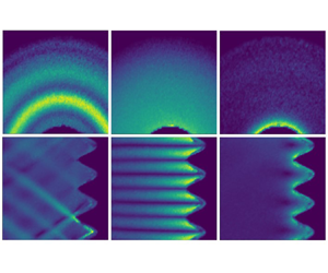
(a) Sketch of the experimental apparatus, showing all principal parts of the experiment. A wave generator with sinusoidal topography is used to excite inertial waves with angular frequency $\varpi$. (b) Amplitude of the velocity in vertical (left column) and horizontal (right column) planes for three oscillation frequencies: $\varpi /2\varOmega \approx 0.72$ (top), $\varpi /2\varOmega \approx 1$ (middle) and $\varpi /2\varOmega \approx 1.5$ (bottom). We have normalized each panel by its maximum amplitude of velocity.

The inviscid vorticity equation in the rotating frame is (Davidson Reference Davidson2013)

(2.4)\begin{equation} \frac{\partial \boldsymbol{\omega}}{\partial t} = 2( \boldsymbol{\varOmega}\boldsymbol{\cdot}\boldsymbol{\nabla})\boldsymbol{u}, \end{equation}

where $\boldsymbol {\omega }$ denotes the vorticity, and the application of the operator $\boldsymbol {\nabla } \times (\partial /\partial t)$ to (2.4) yields the well-known wave-like equation for inertial waves,

(2.5)\begin{equation} \frac{\partial^2}{\partial t^2}\nabla^2\boldsymbol{u} + (2\boldsymbol{\varOmega}\boldsymbol{\cdot}\boldsymbol{\nabla})^2\boldsymbol{u} = 0, \end{equation}

with dispersion relation $\varpi /2\varOmega =k_z/|\boldsymbol {k}|$. For axisymmetric flows the $\theta$ component of $\nabla ^2 \boldsymbol {u}$ is

(2.6)\begin{equation} (\nabla^2\boldsymbol{u})_\theta = \frac{1}{r}\nabla^2_* \varGamma, \end{equation}

and so the azimuthal component of our wave equation can be written in the form

(2.7)\begin{equation} \frac{\partial^2}{\partial t^2}\nabla^2_* \varGamma +(2\varOmega)^2\frac{\partial^2 \varGamma}{\partial z^2} = 0, \end{equation}

where

(2.8)\begin{equation} \nabla^2_* = r\frac{\partial}{\partial r}\frac{1}{r}\frac{\partial}{\partial r}+\frac{\partial^2}{\partial z^2} \end{equation}

is the Stokes operator. It is readily confirmed that $\varPsi$ is governed by exactly the same equation.

Consider first the evanescent case of $\varpi > 2\varOmega$. Given the boundary condition (2.3), we look for disturbances of the form

(2.9)\begin{equation} \varGamma = r\hat{u}_\theta(r)\cos(k_z z)\exp(\kern0.06em j\varpi t), \end{equation}

and (2.7) then yields

(2.10)\begin{equation} r^2\hat{u}^{\prime \prime}_\theta(r)+r\hat{u}^\prime_\theta(r) - \hat{u}_\theta -(r\gamma)^2\hat{u}_\theta = 0, \end{equation}

where

(2.11)\begin{equation} \gamma = k_z\sqrt{1-(2\varOmega/\varpi)^2}. \end{equation}

This can be rewritten as

(2.12)\begin{equation} s^2\hat{u}^{\prime \prime}_\theta(s)+s\hat{u}^\prime_\theta(s) - (s^2+1) \hat{u}_\theta = 0,\quad s = \gamma r, \end{equation}

which has the general solution

(2.13)\begin{equation} \hat{u}_\theta= AK_1(s)+BI_1(s), \end{equation}

where $K_1$ and $I_1$ are the usual exponential-like modified Bessel functions and $A$ and $B$ are constants. Moreover, $u_r$ can be found from $u_\theta$ using the azimuthal component of the Euler equation:

(2.14)\begin{equation} \frac{\partial \varGamma}{\partial t} ={-} 2 \varOmega r u_r. \end{equation}

It remains to combine (2.14) with (2.3) to give the boundary condition at $R_1$,

(2.15a,b)\begin{equation} u_\theta ={-}2\varOmega\eta,\quad r=R_1, \end{equation}

which, along with the boundary condition $u_r = u_\theta = 0$ at $R_2$ , allows us to determine the two unknown coefficients in (2.13). In particular, $u_\theta = 0$ at $R_2$ demands

(2.16)\begin{equation} u_\theta = A\left[K_1(\gamma r)-\frac{K_1(\gamma R_2)}{I_1(\gamma R_2)}I_1(\gamma r) \right] \cos(k_z z)\cos(\varpi t), \end{equation}

while (2.15a,b) yields

(2.17)\begin{equation} A ={-}2\varOmega\hat{\eta} \frac{I_1(\gamma R_2)}{I_1(\gamma R_2)K_1(\gamma R_1)-I_1(\gamma R_1)K_1(\gamma R_2)}. \end{equation}

Finally, (2.14) gives us

(2.18)\begin{equation} u_r = A \frac{\varpi}{2\varOmega} \left[K_1(\gamma r)-\frac{K_1(\gamma R_2)}{I_1(\gamma R_2)}I_1(\gamma r)\right]\cos(k_z z)\sin(\varpi t), \end{equation}

which we integrate to give

(2.19)\begin{equation} \varPsi ={-}A \frac{\varpi r}{2\varOmega k_z}\left[K_1(\gamma r)-\frac{K_1(\gamma R_2)}{I_1(\gamma R_2)}I_1(\gamma r)\right]\sin(k_z z)\sin(\varpi t). \end{equation}

These expressions all relate to evanescent disturbances. The equivalent results for inertial waves can be obtained by returning to (2.7) and (2.10) and taking $\varpi <2\varOmega$. Introducing

(2.20)\begin{equation} \beta = k_z\sqrt{(2\varOmega/\varpi)^2-1}, \end{equation}

and following the same steps as above, we find

(2.21)\begin{gather} u_\theta = A^*\left[Y_1(\beta r) - \frac{Y_1(\beta R_2)}{J_1(\beta R_2)}J_1(\beta r)\right] \cos(k_z z)\cos(\varpi t), \end{gather}

(2.22)\begin{gather}u_r = A^*\frac{\varpi}{2\varOmega}\left[Y_1(\beta r) - \frac{Y_1(\beta R_2)}{J_1(\beta R_2)}J_1(\beta r)\right] \cos(k_z z)\sin(\varpi t), \end{gather}

where $Y_1$ and $J_1$ are the usual oscillatory Bessel functions and

(2.23)\begin{equation} A^*={-}2\varOmega\hat{\eta}\frac{J_1(\beta R_2)}{J_1(\beta R_2) Y_1(\beta R_1)-J_1(\beta R_1)Y_1(\beta R_2)}. \end{equation}

Finally, it is of interest to consider what happens as we approach the cross-over frequency $\varpi = 2\varOmega$ from above and below. It is readily confirmed that, if we let $\varpi \rightarrow 2\varOmega$ in either (2.16) or (2.21), we find

(2.24)\begin{equation} u_\theta \sim{-}2\varOmega\hat{\eta}\frac{R_1}{r}\frac{R_2^2-r^2}{R^2_2-R^2_1}\cos(k_z z)\cos(2\varOmega t). \end{equation}

Evidently, there is a smooth transition from inertial waves to evanescent disturbances at $\varpi = 2\varOmega$. Moreover, at the cross-over frequency, the radial variation in velocity is neither oscillatory nor exponential, but a simple power law. For example, the angular momentum density, $\varGamma$, falls monotonically from a maximum at the inner boundary to zero at the outer boundary, according to $\varGamma \sim (R^2_2 -r^2)\cos (k_z z)\cos (2\varOmega t)$.

3. The experimental set-up

Let us now turn to the experiment. Figure 1(a) shows the experimental set-up. A closed cylindrical tank of radius $R_2 = 14$ cm and height $H = 28.5$ cm is completely filled with water and mounted on a turntable rotating at an angular velocity of $\varOmega = 3.14$ rad s$^{-1}$. To excite wave motion, we use a wave generator in the form of a cylindrically-shaped shaft of mean radius $R_1 = 3.99$ cm, and with a sinusoidal surface of vertical wavelength $\lambda = 2.86$ cm and radial amplitude $\eta _0 = 0.79$ cm. The wave generator is oscillated up and down the rotation axis with a frequency of $4.52\ \text {rad}\ \text {s}^{-1} < \varpi < 9.42$ rad s$^{-1}$ and amplitude $z_0 = 0.5$ mm by a servo motor and a cam. The choice of a small displacement amplitude is motivated by our interest in studying the laminar flow response without inducing any instabilities, which should be a safe assumption at our Rossby numbers $Ro=\varpi \hat {\eta }/(\varOmega R_1) < 0.02$.

As a consequence of this oscillation, the inner boundary is perturbed radially according to

(3.1)\begin{equation} \eta(z,t)={-}\eta_0 \sin[ k_z(z-\delta z(t))],\quad \delta z = z_0 \cos(\varpi t), \end{equation}

where $k_z = 2{\rm \pi} /\lambda$. For $k_z z_0 \ll 1$, the inner boundary condition can be linearized to give

(3.2)\begin{equation} \eta(z,t)={-}\eta_0 \sin(k_z z) + (k_z z_0 \eta_0)\cos(k_z z) \cos (\varpi t), \end{equation}

the time-dependant part of which we rewrite as

(3.3)\begin{equation} \eta(z,t) = \hat{\eta} \cos(k_z z) \cos(\varpi t),\quad \hat{\eta} = k_z z_0 \eta_0. \end{equation}

For quantitative flow visualization we use Particle Image Velocimetry (PIV) in horizontal and vertical planes. We seed the fluid with hollow glass spheres of diameter $15\ \mathrm {\mu }\text {m}$ and density $1050$ kg m$^{-3}$. The particles are illuminated by a 1 watt continuous green laser and a line generator lens, which can provide a horizontal and vertical laser light sheet. We position the horizontal laser light sheet at mid-height and the vertical laser light sheet along a meridional plane of the cylinder. Note that we align the horizontal laser light sheet with the plane of maximum velocity of the excited waves. A MicroVec camera equipped with a Nikon$^\text {TM}$ $50$ mm lens is used to record images of $2592\times 2048$ pixels at 30 frames per second. We use the PIV package DPIVsoft2010 (Meunier & Leweke Reference Meunier and Leweke2003) to calculate velocity fields with $320\times 232$ vectors over an area equivalent of $14.5\times 11.5$ cm.

Our experimental protocol is as follows: we set the turntable into rotation at $3.14$ rad s$^{-1}$ and wait until the fluid is co-rotating with the container. We then start the motion of the wave generator at angular frequency $\varpi$ and wait for the initial transient motion to be dissipated. Finally, we start our PIV measurements and sample a time series of 1200 images, typically ${\sim }40$ oscillations of the wave generator.

In figure 1, we provide a qualitative impression of the flow excited by the wave generator at three different frequencies, to illustrate the three different regimes. For $\varpi < 2\varOmega$, we see inertial waves with a characteristic ray pattern orthogonal to the wavevector $\boldsymbol {k}$, which in turn satisfies the dispersion relation $\varpi /2\varOmega = k_z/|\boldsymbol {k}| = \cos \varphi$. As the excitation frequency approaches the limit $\varpi \rightarrow 2\varOmega$, the group velocity $\boldsymbol {c}_g$ becomes horizontal, and so the characteristic surfaces along which the energy travels are also horizontal, with a wavevector parallel to the rotation axis, $\varphi = 0$. Note that the same disturbance pattern is obtained if we approach $\varpi = 2\varOmega$ from above, so we could equally regard the horizontal striations in this image as indicative of evanescent waves. Finally, for $\varpi > 2\varOmega$ the energy does not propagate into the bulk but remains confined to the vicinity of the wave generator, except, of course, as we approach the limit $\varpi \rightarrow 2\varOmega$.

4. Evanescent disturbances and standing waves near the cross-over frequency

To compare the inviscid predictions with our experimental results, we first consider the radial profile of kinetic energy density in the equatorial plane. We construct radial profiles of the kinetic energy by averaging the kinetic energy density over the azimuth in each PIV frame. The average is calculated over thin concentric rings of radial thickness $1$ mm, resulting in a radial profile of the kinetic energy density with 90 data points. Each data point represents the azimuthal average of at least 300 individual points close to the wave generator and up to 800 points in the outer regions. Finally, we average the time-resolved radial profiles over approximately 40 cycles of the wave generator motion. The resulting radial profiles are displayed in figure 2.

Figure 2.

Kinetic energy density as a function of the radial distance for different driving frequencies. The value above each line represents the ratio $\varpi /2\varOmega$. Each curve on the left is offset by $0.4$, while those in the middle and right are offset by $0.6$, to achieve better visibility. Crossed points depict the measurements. The dashed lines represent the inviscid solution, while solid lines represent the solution with a viscous correction, as discussed in §§ 5 and 6.

The inviscid analysis described in § 2 predicts exponentially decaying evanescent waves for $\varpi > 2 \varOmega$. Consistent with this, the experimental data for excitation frequencies significantly above $2\varOmega$ (figure 2a) shows that the kinetic energy is mostly confined to the vicinity of the wave generator, from where it decays exponentially with the radius. However, even at $\varpi /2\varOmega \sim 1.5$, the energy of the evanescent waves still penetrates into the bulk up to around 10 % of the fluid gap. All in all, the predicted inviscid solution for $\boldsymbol {u}$ is in good agreement with the radial structure of the measured kinetic energy, as displayed in figure 2(a).

We now turn to excitation frequencies which are close to, but above, the critical value of $\varpi = 2\varOmega$ (figure 2b). Again, there is a close link between theory and measurements, with the radial profiles of the kinetic energy becoming flatter as we approach the cross-over frequency, which means that the motion progressively spreads away from the wave generator. This observation, while consistent with our inviscid analysis, contrasts with the early study of Morgan (Reference Morgan1951). Morgan investigated theoretically the problem of an oscillating disk in a cylindrical geometry and found that, as the excitation frequency gets close to the critical value of $2\varOmega$, the fluid motion is mostly confined to the vicinity of the disk. He speculates about a resonant behaviour resulting in ‘violent motion’ when the system is excited at exactly the critical frequency. Baines (Reference Baines1967), on the other hand, concludes that no steady-state solution exists in this limit. In contrast to these statements, we observe a smooth transition from evanescent waves with radially decaying velocity to a standing-wave profile as $\varpi$ passes through the cross-over frequency of $2\varOmega$ (figure 2c). We therefore conclude that, at least for the type of forcing used in our experiment, there is no unusual behaviour at $\varpi = 2\varOmega$. Rather, there is a smooth transition, exactly as predicted by the inviscid analysis. Interestingly, figure 2(c) shows a significant discrepancy between the inviscid analysis and the measurements when $\varpi < 2\varOmega$, particularly at $\varpi /2\varOmega = 0.991$. We shall see shortly that this is due to a standing-wave resonance whose amplitude is controlled by viscosity.

Also shown in figure 2(a–c) are the viscous corrections to the inviscid theory. These corrections are negligible in the evanescent regime, but important below the cross-over frequency. We shall discuss these corrections, as well as the discrepancy between the inviscid theory and observations for $\varpi < 2\varOmega$, in § 6.

5. Corrections due to viscous action in the bulk

When viscosity is finite, (2.14) generalizes to

(5.1)\begin{equation} \left(\frac{\partial}{\partial t}-\nu \nabla^2_* \right)\varGamma ={-} 2 \varOmega r u_r, \end{equation}

while the azimuthal component of

(5.2)\begin{equation} \frac{\partial \boldsymbol{\omega}}{\partial t} = 2( \boldsymbol{\varOmega}\boldsymbol{\cdot}\boldsymbol{\nabla})\boldsymbol{u} + \nu \nabla^2 \boldsymbol{\omega} \end{equation}

combines with

(5.3)\begin{equation} (\nabla^2\boldsymbol{\omega})_\theta = \frac{1}{r}\nabla^2_* (r\omega_\theta), \end{equation}

to yield

(5.4)\begin{equation} \left(\frac{\partial}{\partial t}-\nu\nabla^2_* \right) r \omega_\theta = 2\varOmega \frac{\partial \varGamma}{\partial z}. \end{equation}

It is convenient to introduce the Stokes streamfunction, $\varPsi$, defined by (2.1). This gives us

(5.5a,b)\begin{equation} u_r ={-}\frac{1}{r}\frac{\partial \varPsi}{\partial z},\quad r\omega_\theta ={-}\nabla^2_*\varPsi, \end{equation}

and so (5.1) and (5.4) become

(5.6)\begin{gather} \left(\frac{\partial}{\partial t} - \nu \nabla^2_*\right) \varGamma = 2\varOmega \frac{\partial \varPsi}{\partial z}, \end{gather}

(5.7)\begin{gather}\left(\frac{\partial}{\partial t} - \nu \nabla^2_*\right) \nabla^2_* \varPsi ={-}2\varOmega \frac{\partial \varGamma}{\partial z}. \end{gather}

These, in turn, yield

(5.8)\begin{equation} \left(\frac{\partial}{\partial t} - \nu \nabla^2_*\right)^2\nabla^2_*\varGamma + (2\varOmega)^2\frac{\partial^2 \varGamma}{\partial z^2}=0, \end{equation}

which is the viscous generalization of (2.7), as well as

(5.9)\begin{equation} \left(\frac{\partial}{\partial t} - \nu \nabla^2_*\right)^2\nabla^2_*\varPsi + (2\varOmega)^2\frac{\partial^2 \varPsi}{\partial z^2}=0. \end{equation}

As with the inviscid analysis, we can work with either $\varGamma$ or $\varPsi$, but for the viscous case it is easier to work with $\varPsi$. The boundary condition (2.3) can be rewritten in terms of $\varPsi$ as

(5.10)\begin{equation} u_r(z,t)=\frac{\partial \eta}{\partial t} ={-} \frac{1}{r}\frac{\partial \varPsi}{\partial z}, \end{equation}

which combines with (2.2) to give

(5.11)\begin{equation} \varPsi(R_1,z,t)= \hat{\eta} \frac{\varpi R_1}{k_z}\sin(k_z z)\sin(\varpi t). \end{equation}

We therefore look for standing waves or evanescent disturbances of the form

(5.12)\begin{equation} \varPsi = \hat{\varPsi}(r)\sin(k_z z) \exp(\kern0.06em {j} \varpi t),\end{equation}

where $\hat {\varPsi }$ is complex. The expression (5.12) combines with (5.9) to give

(5.13)\begin{equation} \left[1+j\left(\frac{\nu k_z^2}{\varpi}\right)(\hat{\nabla}^2_*-1)\right]^2 (\hat{\nabla}^2_*-1)\hat{\varPsi} + \left(\frac{2\varOmega}{\varpi}\right)^2 \hat{\varPsi} = 0, \end{equation}

where the dimensionless operator is

(5.14)\begin{equation} \hat{\nabla}_*^2 = \frac{1}{k_{z}^2}r\frac{\partial}{\partial r}\frac{1}{r}\frac{\partial}{\partial r}. \end{equation}

At this point we can look for either evanescent disturbances or standing inertial waves. Let us consider evanescent disturbances. For $\varpi > 2\varOmega$, (5.13) admits solutions of the form

(5.15)\begin{equation} \hat{\varPsi} = CrK_1(\kappa k_z r) + DrI_1(\kappa k_z r), \end{equation}

provided

(5.16)\begin{equation} \left[1+{j}\left(\frac{\nu k_z^2}{\varpi}\right)(\kappa^2-1)\right]^2(\kappa^2-1)+ \left(\frac{2\varOmega}{\varpi}\right)^2 = 0. \end{equation}

Note that, when $\nu = 0$, (5.16) reduces to

(5.17)\begin{equation} \kappa = \kappa_0 = \sqrt{1-(2\varOmega/ \varpi)^2} = \gamma/k_z, \end{equation}

and so we recover the inviscid solution. For small $\nu k^2_z / \varpi$, which is the case in our experiment, (5.16) has the solution

(5.18)\begin{equation} \kappa^2 = \left[1-\left(\frac{2\varOmega}{\varpi}\right)^2\right] - 2{j}\left(\frac{\nu k^2_z}{\varpi}\right)\left(\frac{2\varOmega}{\varpi}\right)^4 + O ((\nu k_z^2/\varpi)^2). \end{equation}

We can use this estimate of $\kappa$, along with (5.15), to estimate the effects of viscosity on evanescent disturbances. The equivalent results for inertial waves may be found in exactly the same way.

6. A comparison of the measurements with the viscously corrected theory

We can use the analysis above to estimate the effects of viscosity on the propagation of both inertial waves and evanescent disturbances. We shall do this while ignoring the viscous boundary layer on the wave generator, of which an estimate of the thickness and local Reynolds number are $\delta \sim \sqrt {\nu /\varOmega } \approx 0.6$ mm and $Re = u \delta /\nu = (\varpi \hat {\eta })\delta /\nu \approx 1.8$. That is to say, we shall assume, and then check retrospectively, that viscosity does not strongly influence the generation of inertial waves or evanescent disturbances, only their subsequent behaviour in the bulk. To that end, we use (5.18) to evaluate $\kappa$, substitute this into (5.15), and then use the inviscid estimates for the coefficients $C$ and $D$ taken from (2.19). A similar procedure can be followed for inertial waves. A comparison of these viscous corrections with the experimental data is shown in figure 2, where the viscously-corrected predictions are the solid lines.

In our experiment we have $\nu k_z^2 / \varpi \approx 0.008$ and so we might expect the viscous corrections to be modest for $\varpi = 2\varOmega$. Moreover, the inviscid and viscously corrected theory seem to capture equally well the experimental data in the evanescent regime, $\varpi > 2\varOmega$. This suggests that the evanescent disturbances are not strongly influenced by viscosity, at least not in our experiment. However, the superiority of the viscously corrected solutions over the inviscid predictions is particularly clear when $\varpi$ is somewhat less than $2\varOmega$ (figure 2c). Here the inviscid solution is less successful at capturing the radial structure of the flow, and this is especially true when we are close to a resonance of the standing waves, as is the case for $\varpi /2\varOmega = 0.991$.

To show that this discrepancy between the inviscid theory and the observations arises from a resonance, we investigate the dependence of the total kinetic energy on $\varpi /2\varOmega$. We consider the total mean kinetic energy over the entire PIV image averaged over 40 oscillation periods and plot it against its analytical counterpart for various excitation frequencies. The results are presented in figure 3(a), where the dashed line represents the inviscid theory and the solid line the viscously corrected prediction. Evidently, there is a quantitative agreement between the viscous theory and experiments, but a large discrepancy with the inviscid theory at around $\varpi /2\varOmega \approx 0.99$. This frequency corresponds to the denominator in (2.17) falling to zero, and so represents a geometrical resonance in the standing wave pattern. Clearly, this resonance is smoothed out by viscosity.

Figure 3.

(a) The kinetic energy calculated from the velocity amplitude over the PIV area as a function of $\varpi /2\varOmega$. The solid line represents the viscous prediction, the coloured dots the measurements, and the dashed line the inviscid solution. (b) The peak in energy at $\varpi / 2\varOmega \approx 0.99$ corresponds to a geometric resonance between emitted and reflected waves at critical angle $\varphi _1$.

Physically, this resonant frequency corresponds to inertial waves reflected from the outer wall interfering constructively with outgoing waves, according to the expression

(6.1)\begin{equation} \frac{\varpi}{2\varOmega} = \frac{R_2-R_1}{\sqrt{(R_2-R_1)^2 + (\lambda/2)^2}}. \end{equation}

This is illustrated in figure 3(b). Further resonances are expected with the frequencies

(6.2)\begin{equation} \frac{\varpi_n}{2\varOmega} = \frac{R_2-R_1}{\sqrt{(R_2-R_1)^2 + (n\lambda/2)^2}}. \end{equation}