


1. Introduction
The incompressible flow inside a square cavity, driven by the tangential motion of one of its sides, has long served as a model problem in fluid mechanics (Shankar & Deshpande Reference Shankar and Deshpande2000; Kuhlmann & Romanò Reference Kuhlmann and Romanò2019) for the study of wall-bounded vortex dynamics, centrifugal and shear flow instabilities, or laminar–turbulent transition within enclosed containers, to name but a few complex flow phenomena of interest. Because of its compelling simplicity, the so-called lid-driven square cavity (LDSC) flow problem, has readily become a classic benchmark for the validation of numerical codes that solve the Navier–Stokes equations (Ghia, Ghia & Shin Reference Ghia, Ghia and Shin1982; Schreiber & Keller Reference Schreiber and Keller1983; Vanka Reference Vanka1986; Gresho & Chan Reference Gresho and Chan1990; Hou et al. Reference Hou, Zou, Chen, Doolen and Cogley1995; Botella & Peyret Reference Botella and Peyret1998; Auteri et al. Reference Auteri, Quartapelle and Vigevano2002b ; Sahin & Owens Reference Sahin and Owens2003a ; Gupta & Kalita Reference Gupta and Kalita2005; Bruneau & Saad Reference Bruneau and Saad2006; Marchi, Suero & Araki Reference Marchi, Suero and Araki2009; Khorasanizade & Sousa Reference Khorasanizade and Sousa2014; Romanò & Kuhlmann Reference Romanò and Kuhlmann2017).
Although the first instability of the LDSC base flow in an infinite-span domain is three-dimensional (3-D) in nature (Koseff & Street Reference Koseff and Street1984; Aidun, Triantafillopoulos & Benson Reference Aidun, Triantafillopoulos and Benson1991; Benson & Aidun Reference Benson and Aidun1992; Albensoeder, Kuhlmann & Rath Reference Albensoeder, Kuhlmann and Rath2001; Theofilis, Duck & Owen Reference Theofilis, Duck and Owen2004; Non, Pierre & Gervais Reference Non, Pierre and Gervais2006), which corresponds to a disruption of the translational spanwise invariance that results in an infinite array of steady Taylor–Görtler vortices of wavenumber $\kappa _{3D}\simeq 15.4\,L^{-1}$
beyond
$\kappa _{3D}\simeq 15.4\,L^{-1}$
beyond $ \textit{Re}_{3D}= \textit{LU}/\nu \simeq 785$
, the purely two-dimensional (2-D) bifurcation scenario constitutes a much more convenient set-up for benchmarking hydrodynamic stability codes. Here,
$ \textit{Re}_{3D}= \textit{LU}/\nu \simeq 785$
, the purely two-dimensional (2-D) bifurcation scenario constitutes a much more convenient set-up for benchmarking hydrodynamic stability codes. Here, $L$
is the streamwise size of the lid,
$L$
is the streamwise size of the lid, $U$
its sliding velocity and
$U$
its sliding velocity and $\nu$
the kinematic viscosity of the fluid.
$\nu$
the kinematic viscosity of the fluid.
Regularisation of the sliding lid boundary condition to avoid the singularity at the corners has the 2-D LDSC first destabilise in a supercritical Hopf bifurcation at $\textit{Re}_H= 10\,267\pm 12$
with non-dimensional angular frequency
$\textit{Re}_H= 10\,267\pm 12$
with non-dimensional angular frequency $\omega _H\simeq 2.080\,L/U$
(Shen Reference Shen1991; Fortin et al. Reference Fortin, Jardak, Gervais and Pierre1997; Abouhamza & Pierre Reference Abouhamza and Pierre2003). The type and nature of the bifurcation remains the same for LDSC with corner singularities, but the instability is promoted to
$\omega _H\simeq 2.080\,L/U$
(Shen Reference Shen1991; Fortin et al. Reference Fortin, Jardak, Gervais and Pierre1997; Abouhamza & Pierre Reference Abouhamza and Pierre2003). The type and nature of the bifurcation remains the same for LDSC with corner singularities, but the instability is promoted to $\textit{Re}_H\simeq 8020$
and the angular frequency higher at
$\textit{Re}_H\simeq 8020$
and the angular frequency higher at $\omega _H\simeq 2.83\,L/U$
(Poliashenko & Aidun Reference Poliashenko and Aidun1995; Fortin et al. Reference Fortin, Jardak, Gervais and Pierre1997; Cazemier, Verstappen & Veldman Reference Cazemier, Verstappen and Veldman1998; Tiesinga, Wubs & Veldman Reference Tiesinga, Wubs and Veldman2002; Abouhamza & Pierre Reference Abouhamza and Pierre2003; Peng, Shiau & Hwang Reference Peng, Shiau and Hwang2003; Sahin & Owens Reference Sahin and Owens2003b
; Bruneau & Saad Reference Bruneau and Saad2006; Boppana & Gajjar Reference Boppana and Gajjar2010; Kalita & Gogoi Reference Kalita and Gogoi2016; Nuriev, Egorov & Zaitseva Reference Nuriev, Egorov and Zaitseva2016; Murdock, Ickes & Yang Reference Murdock, Ickes and Yang2017).
$\omega _H\simeq 2.83\,L/U$
(Poliashenko & Aidun Reference Poliashenko and Aidun1995; Fortin et al. Reference Fortin, Jardak, Gervais and Pierre1997; Cazemier, Verstappen & Veldman Reference Cazemier, Verstappen and Veldman1998; Tiesinga, Wubs & Veldman Reference Tiesinga, Wubs and Veldman2002; Abouhamza & Pierre Reference Abouhamza and Pierre2003; Peng, Shiau & Hwang Reference Peng, Shiau and Hwang2003; Sahin & Owens Reference Sahin and Owens2003b
; Bruneau & Saad Reference Bruneau and Saad2006; Boppana & Gajjar Reference Boppana and Gajjar2010; Kalita & Gogoi Reference Kalita and Gogoi2016; Nuriev, Egorov & Zaitseva Reference Nuriev, Egorov and Zaitseva2016; Murdock, Ickes & Yang Reference Murdock, Ickes and Yang2017).
The periodic solution resulting from the Hopf bifurcation undergoes a Neimark–Sacker bifurcation at $\textit{Re}_{N\!S}\simeq 9150$
with modulational frequency
$\textit{Re}_{N\!S}\simeq 9150$
with modulational frequency $\omega _{N\!S}\simeq 1.7\,L/U$
(Tiesinga et al. Reference Tiesinga, Wubs and Veldman2002), in fair agreement with the characteristic properties of quasiperiodic solutions reported in the literature at slightly higher Reynolds numbers (Poliashenko & Aidun Reference Poliashenko and Aidun1995; Cazemier et al. Reference Cazemier, Verstappen and Veldman1998; Auteri et al. Reference Auteri, Parolini and Quartapelle2002a
). An analysis of the steady state beyond the original Hopf instability reveals a sequence of further supercritical Hopf bifurcations whose properties anticipate the upcoming Neimark–Sacker bifurcation (Tiesinga et al. Reference Tiesinga, Wubs and Veldman2002). The chaotic dynamics that follows shortly after the emergence of quasi-periodicity have been shown to result from a classic Ruelle–Takens scenario (Ruelle & Takens Reference Ruelle and Takens1971; Newhouse, Ruelle & Takens Reference Newhouse, Ruelle and Takens1978).
$\omega _{N\!S}\simeq 1.7\,L/U$
(Tiesinga et al. Reference Tiesinga, Wubs and Veldman2002), in fair agreement with the characteristic properties of quasiperiodic solutions reported in the literature at slightly higher Reynolds numbers (Poliashenko & Aidun Reference Poliashenko and Aidun1995; Cazemier et al. Reference Cazemier, Verstappen and Veldman1998; Auteri et al. Reference Auteri, Parolini and Quartapelle2002a
). An analysis of the steady state beyond the original Hopf instability reveals a sequence of further supercritical Hopf bifurcations whose properties anticipate the upcoming Neimark–Sacker bifurcation (Tiesinga et al. Reference Tiesinga, Wubs and Veldman2002). The chaotic dynamics that follows shortly after the emergence of quasi-periodicity have been shown to result from a classic Ruelle–Takens scenario (Ruelle & Takens Reference Ruelle and Takens1971; Newhouse, Ruelle & Takens Reference Newhouse, Ruelle and Takens1978).
This is a rather dull bifurcation sequence that does not provide all necessary ingredients to test hydrodynamic stability codes to their fullest. In particular, it lacks fold bifurcations, which are required to validate steady and periodic state continuation codes, or global bifurcations involving homoclinic or heteroclinic orbits. Furthermore, the first bifurcation occurs at a rather large value of the Reynolds number, which poses a further complication by requiring particularly fine space and time discretisations, and the ensuing need of intensive computational resources. Finally, the problem lacks any kind of symmetries, such that no allowance is made for the appearance of the rich bifurcation scenarios that typically arise in their presence.
All three shortcomings can be overcome by simply setting a second or all four walls of the square cavity in motion. This increases the parameter count to two and four, respectively, and, by setting all lid velocities to the same value or to two different values in pairs, symmetries might be introduced that greatly enrich the dynamics of the problem. In the case of all four walls moving at the same velocity, with facing walls sliding in opposite directions, transitional dynamics are brought to much lower $ \textit{Re}$
and become particularly complex. The model is, from a mathematical standpoint, as simple as the classic LDSC flow problem, but provides a much broader benchmark for testing numerical schemes intended for the continuation of solution branches and the analysis of all sorts of bifurcations, both local and global, in the presence or absence of symmetries.
$ \textit{Re}$
and become particularly complex. The model is, from a mathematical standpoint, as simple as the classic LDSC flow problem, but provides a much broader benchmark for testing numerical schemes intended for the continuation of solution branches and the analysis of all sorts of bifurcations, both local and global, in the presence or absence of symmetries.
The 4-lid-driven symmetric square cavity (4LDSSC) flow undergoes a symmetry-breaking steady bifurcation at $ \textit{Re}_{P_1}\simeq 129$
that results in two branches of mutually symmetric solutions (Wahba 2009; Perumal & Dass Reference Perumal and Dass2011). The mirror symmetry about both diagonals is broken, but an invariance to rotations of angle
$ \textit{Re}_{P_1}\simeq 129$
that results in two branches of mutually symmetric solutions (Wahba 2009; Perumal & Dass Reference Perumal and Dass2011). The mirror symmetry about both diagonals is broken, but an invariance to rotations of angle $\pi$
about the cavity centre persists. While the already unstable branch of symmetric solutions undergoes a second pitchfork bifurcation at
$\pi$
about the cavity centre persists. While the already unstable branch of symmetric solutions undergoes a second pitchfork bifurcation at $ \textit{Re}_{P_2}\simeq 359$
(Cadou, Guevel & Girault Reference Cadou, Guevel and Girault2012; Zhuo et al. Reference Zhuo, Zhong, Guo and Cao2013), both a Hopf (Wahba Reference Wahba2011; Zhuo et al. Reference Zhuo, Zhong, Guo and Cao2013, Reference Zhuo, Zhong, Guo and Cao2015) and a steady bifurcation (Cadou et al. Reference Cadou, Guevel and Girault2012), for which the symmetry-breaking or preserving nature was not specified, have been inconsistently reported for the branch of asymmetric solutions at values of the Reynolds number of
$ \textit{Re}_{P_2}\simeq 359$
(Cadou, Guevel & Girault Reference Cadou, Guevel and Girault2012; Zhuo et al. Reference Zhuo, Zhong, Guo and Cao2013), both a Hopf (Wahba Reference Wahba2011; Zhuo et al. Reference Zhuo, Zhong, Guo and Cao2013, Reference Zhuo, Zhong, Guo and Cao2015) and a steady bifurcation (Cadou et al. Reference Cadou, Guevel and Girault2012), for which the symmetry-breaking or preserving nature was not specified, have been inconsistently reported for the branch of asymmetric solutions at values of the Reynolds number of $ \textit{Re}\simeq 720$
and
$ \textit{Re}\simeq 720$
and $ \textit{Re}\simeq 867$
, respectively. A long period limit cycle has been observed to attract the dynamics beyond the alleged Hopf bifurcation, whose super (Wahba Reference Wahba2011) or subcriticality (Zhuo et al. Reference Zhuo, Zhong, Guo and Cao2013, Reference Zhuo, Zhong, Guo and Cao2015) has not been established. The periodic state, which preserves the
$ \textit{Re}\simeq 867$
, respectively. A long period limit cycle has been observed to attract the dynamics beyond the alleged Hopf bifurcation, whose super (Wahba Reference Wahba2011) or subcriticality (Zhuo et al. Reference Zhuo, Zhong, Guo and Cao2013, Reference Zhuo, Zhong, Guo and Cao2015) has not been established. The periodic state, which preserves the $\pi$
-rotational invariance, evolves in the vicinity of one of the asymmetric steady states for half a period and of its symmetry-conjugate counterpart for the other half, periodically switching from one to the other.
$\pi$
-rotational invariance, evolves in the vicinity of one of the asymmetric steady states for half a period and of its symmetry-conjugate counterpart for the other half, periodically switching from one to the other.
A leap forward in clarifying the bifurcation diagram of the 4LDSSC flow was undertaken by Chen et al. (Reference Chen, Tsai and Luo2013) employing pseudo-arclength continuation and Arnoldi stability analysis of steady states. The first and second pitchfork bifurcations were confirmed at $ \textit{Re}_{P_1}=130.29$
and
$ \textit{Re}_{P_1}=130.29$
and $ \textit{Re}_{P_2}=355.45$
, and the two corresponding branches of asymmetric states found to coalesce in a saddle-node bifurcation at
$ \textit{Re}_{P_2}=355.45$
, and the two corresponding branches of asymmetric states found to coalesce in a saddle-node bifurcation at $ \textit{Re}_{S\!N}=877$
, which might possibly be the secondary steady bifurcation reported by Cadou et al. (Reference Cadou, Guevel and Girault2012). The symmetric steady state, which becomes unstable at the first pitchfork as a pair of stable conjugate-symmetric asymmetric state branches is issued, was found to remain unstable beyond the second pitchfork. At this point, a second pair of unstable asymmetric state branches is created. In contrast to expectation, the stable pair of asymmetric solutions was not seen to undergo a secondary Hopf bifurcation and reached instead the saddle-node bifurcation with their stability intact.
$ \textit{Re}_{S\!N}=877$
, which might possibly be the secondary steady bifurcation reported by Cadou et al. (Reference Cadou, Guevel and Girault2012). The symmetric steady state, which becomes unstable at the first pitchfork as a pair of stable conjugate-symmetric asymmetric state branches is issued, was found to remain unstable beyond the second pitchfork. At this point, a second pair of unstable asymmetric state branches is created. In contrast to expectation, the stable pair of asymmetric solutions was not seen to undergo a secondary Hopf bifurcation and reached instead the saddle-node bifurcation with their stability intact.
Regardless of the occurrence or otherwise of a Hopf bifurcation, no stable steady state remains beyond the saddle-node bifurcation. The aforementioned periodic orbit is left as the only stable solution for a moderate $ \textit{Re}$
range before eventually triggering the onset of chaotic dynamics. It is one of the main aims of this paper to elucidate the origin of this periodic solution, seemingly disconnected from the base symmetric state, in terms of global bifurcations involving the various known solutions, and to clarify how the two disjoint symmetrical regions of phase space, each with its own symmetry-related objects, become dynamically connected. In this respect, the 2-D 4LDSSC problem serves as one of the simplest flow set-ups to illustrate a mechanism whereby statistical symmetry is eventually recovered after a temporary loss. This mechanism may be at play in more complex, experimentally realisable, 3-D flows belonging to the class of problems in fluid mechanics that feature mirror symmetries. Specifically, those that undergo an intermediate regime of stable symmetry-breaking solution branches between the symmetric base state that acts as the global attractor at low
$ \textit{Re}$
range before eventually triggering the onset of chaotic dynamics. It is one of the main aims of this paper to elucidate the origin of this periodic solution, seemingly disconnected from the base symmetric state, in terms of global bifurcations involving the various known solutions, and to clarify how the two disjoint symmetrical regions of phase space, each with its own symmetry-related objects, become dynamically connected. In this respect, the 2-D 4LDSSC problem serves as one of the simplest flow set-ups to illustrate a mechanism whereby statistical symmetry is eventually recovered after a temporary loss. This mechanism may be at play in more complex, experimentally realisable, 3-D flows belonging to the class of problems in fluid mechanics that feature mirror symmetries. Specifically, those that undergo an intermediate regime of stable symmetry-breaking solution branches between the symmetric base state that acts as the global attractor at low $ \textit{Re}$
and the statistically symmetric turbulent (or chaotic) state observed at high
$ \textit{Re}$
and the statistically symmetric turbulent (or chaotic) state observed at high $ \textit{Re}$
. See, for example, the spiral and turbulent spiral regimes in the Taylor–Couette system, separating the stability regions of the circular Couette flow and featureless turbulence (Coles Reference Coles1965; Andereck, Liu & Swinney Reference Andereck, Liu and Swinney1986; Meseguer et al. Reference Meseguer, Mellibovsky, Avila and Marques2009; Wang et al. Reference Wang, Mellibovsky, Ayats, Deguchi and Meseguer2023).
$ \textit{Re}$
. See, for example, the spiral and turbulent spiral regimes in the Taylor–Couette system, separating the stability regions of the circular Couette flow and featureless turbulence (Coles Reference Coles1965; Andereck, Liu & Swinney Reference Andereck, Liu and Swinney1986; Meseguer et al. Reference Meseguer, Mellibovsky, Avila and Marques2009; Wang et al. Reference Wang, Mellibovsky, Ayats, Deguchi and Meseguer2023).
3-D 4LDSSC bounded in the spanwise direction by stationary walls has been shown to preserve, for low aspect ratios, the problem symmetry to higher $ \textit{Re}$
as compared with 2-D simulations (Li & Maa Reference Li and Maa2017). The stabilising effect of the walls is reduced as the aspect ratio is increased and the critical
$ \textit{Re}$
as compared with 2-D simulations (Li & Maa Reference Li and Maa2017). The stabilising effect of the walls is reduced as the aspect ratio is increased and the critical $ \textit{Re}_{P_1}$
for the symmetry breaking bifurcation diminishes, but remains high at 319 for an aspect ratio of 3. The flow patterns at midspan are, however, topologically close to those of the 2-D cavity in both the pre- and post-critical regimes. It is nevertheless unclear whether the infinite-span case will remain 2-D across much of the bifurcation scenario reported in the literature. Be it as it might, the low-
$ \textit{Re}_{P_1}$
for the symmetry breaking bifurcation diminishes, but remains high at 319 for an aspect ratio of 3. The flow patterns at midspan are, however, topologically close to those of the 2-D cavity in both the pre- and post-critical regimes. It is nevertheless unclear whether the infinite-span case will remain 2-D across much of the bifurcation scenario reported in the literature. Be it as it might, the low- $ \textit{Re}$
flow dynamics in 2-D cavities is relevant to the understanding of the onset of 2-D turbulence (Molenaar, Clercx & van Heijst Reference Molenaar, Clercx and van Heijst2005), an active research field on account of its sharing key features with the large-scale motions observed in geophysical flows (Boffetta & Ecke Reference Boffetta and Ecke2012). Wall-bounded 2-D vortices do indeed occur in near-shore zones, such as at the head of rip currents (Smith & Largier Reference Smith and Largier1995) or in tidal channels (Wells & van Heijst Reference Wells and van Heijst2003). In particular, the flow set-up we have adopted serves as a simple model for the onset of chaos, a necessary step towards 2-D turbulence, when the base flow consists of two strong opposing jets (issued in our case from the two corners where the lids run into each other) that meet at the centre of a narrowly confined domain. Furthermore, the relevance of analysing bifurcation sequences of unstable solutions in symmetry-restricted domains reaches much further than its mere use for code validation or as a model for the onset of 2-D turbulence. The strange saddle that is embedded in chaotic motion, and therefore organises turbulent dynamics, consists of collections of unstable solutions and their connecting manifolds (Procaccia Reference Procaccia1988). Restricting the analysis to certain symmetries or severely truncated domains, however unrealistic this may appear from a merely experimental point of view, allows for a detailed analysis that is otherwise unattainable and provides access to the basic ingredients that might be at play in the real problem (Hof et al. Reference Hof, van Doorne, Westerweel, Nieuwstadt, Faisst, Eckhardt, Wedin, Kerswell and Waleffe2004; de Lozar et al. Reference de Lozar, Mellibovsky, Avila and Hof2012; Ritter, Mellibovsky & Avila Reference Ritter, Mellibovsky and Avila2016). In the case of systems that feature translational invariance along an extended spatial coordinate, one such possible symmetry-restriction consists in constraining the dynamics to be 2-D (Jimenez Reference Jimenez1990; Mellibovsky & Meseguer Reference Mellibovsky and Meseguer2015).
$ \textit{Re}$
flow dynamics in 2-D cavities is relevant to the understanding of the onset of 2-D turbulence (Molenaar, Clercx & van Heijst Reference Molenaar, Clercx and van Heijst2005), an active research field on account of its sharing key features with the large-scale motions observed in geophysical flows (Boffetta & Ecke Reference Boffetta and Ecke2012). Wall-bounded 2-D vortices do indeed occur in near-shore zones, such as at the head of rip currents (Smith & Largier Reference Smith and Largier1995) or in tidal channels (Wells & van Heijst Reference Wells and van Heijst2003). In particular, the flow set-up we have adopted serves as a simple model for the onset of chaos, a necessary step towards 2-D turbulence, when the base flow consists of two strong opposing jets (issued in our case from the two corners where the lids run into each other) that meet at the centre of a narrowly confined domain. Furthermore, the relevance of analysing bifurcation sequences of unstable solutions in symmetry-restricted domains reaches much further than its mere use for code validation or as a model for the onset of 2-D turbulence. The strange saddle that is embedded in chaotic motion, and therefore organises turbulent dynamics, consists of collections of unstable solutions and their connecting manifolds (Procaccia Reference Procaccia1988). Restricting the analysis to certain symmetries or severely truncated domains, however unrealistic this may appear from a merely experimental point of view, allows for a detailed analysis that is otherwise unattainable and provides access to the basic ingredients that might be at play in the real problem (Hof et al. Reference Hof, van Doorne, Westerweel, Nieuwstadt, Faisst, Eckhardt, Wedin, Kerswell and Waleffe2004; de Lozar et al. Reference de Lozar, Mellibovsky, Avila and Hof2012; Ritter, Mellibovsky & Avila Reference Ritter, Mellibovsky and Avila2016). In the case of systems that feature translational invariance along an extended spatial coordinate, one such possible symmetry-restriction consists in constraining the dynamics to be 2-D (Jimenez Reference Jimenez1990; Mellibovsky & Meseguer Reference Mellibovsky and Meseguer2015).
A notorious complication of simulating the flow inside lid-driven cavities is the infamous singularity at the corners where the sliding lid meets the adjoining stationary walls. Although some studies have devised strategies to soundly address the singularity (Gupta, Manohar & Noble Reference Gupta, Manohar and Noble1981; Botella & Peyret Reference Botella and Peyret2001; Auteri et al. Reference Auteri, Quartapelle and Vigevano2002b
), low-order space discretisations have the advantage of confining its effects to the immediate vicinity of the corners, such that the issue is more often than not disregarded as irrelevant on account of its being of little consequence to the global flow dynamics. High-order discretisations, such as those typically resulting from the use of spectral methods, are however extremely sensitive to the singularity and cannot overlook its decided impact on the bulk flow. A standard fourth-order polynomic regularisation has occasionally been applied to the lid velocity distribution to avoid the singularity (Shen Reference Shen1991; Botella Reference Botella1997) but, although the flow allegedly preserves the qualitative dynamics of the original singular cavity, the quantitative effects are non-negligible. A rather simple means of simulating quasi-singular cavity flows and reduce the quantitative impact to a minimum resorts to the enforcement of a high-order regularisation that achieves a constant velocity over a wider extent of the lid while still removing the singularities at the corners (Batoul, Khallouf & Labrosse Reference Batoul, Khallouf and Labrosse1994). Meseguer et al. (Reference Meseguer, Alonso, Batiste, An and Mellibovsky2024) tackled the 4LDSSC problem with a spectral discretisation and high-order regularisation to unfold the full diagram as regards to steady states and their local bifurcations. In addition to generally confirming the scenario presented by Chen et al. (Reference Chen, Tsai and Luo2013) for the non-regularised case, their detailed analysis further produced hitherto unknown bifurcations and steady solution branches that, unlike all previously known bifurcations and states, also break the $\pi$
rotational symmetry.
$\pi$
rotational symmetry.
Back to the $\pi$
rotationally invariant scenario, and piecing together the states and bifurcations reported in the literature for the 4LDSSC, there seems to be strong evidence advocating for the hypothesis that a degenerate double-zero bifurcation with Z
$\pi$
rotationally invariant scenario, and piecing together the states and bifurcations reported in the literature for the 4LDSSC, there seems to be strong evidence advocating for the hypothesis that a degenerate double-zero bifurcation with Z $_2$
symmetry might be in place. The normal form for this codimension-four bifurcation was first derived by Knobloch (Reference Knobloch1986) and then unfolded by Dangelmayr, Neveling & Armbruster (Reference Dangelmayr, Neveling and Armbruster1986), following earlier work on a partial unfolding of a closely related codimension-three bifurcation by Dangelmayr, Armbruster & Neveling (Reference Dangelmayr, Armbruster and Neveling1985). The associated phase portraits have all the ingredients to explain the observations of the 4LDSSC problem in terms of a one-dimensional (1-D) path across the four-dimensional parameter space in the vicinity of the codimension-four point. In this work, we address the fluid flow problem from a dynamical systems perspective and explore the possible occurrence of a degenerate symmetric double zero bifurcation. Specifically, we are interested in the origin of the long-period space–time-symmetric periodic orbit that is responsible for the onset of chaos at higher
$_2$
symmetry might be in place. The normal form for this codimension-four bifurcation was first derived by Knobloch (Reference Knobloch1986) and then unfolded by Dangelmayr, Neveling & Armbruster (Reference Dangelmayr, Neveling and Armbruster1986), following earlier work on a partial unfolding of a closely related codimension-three bifurcation by Dangelmayr, Armbruster & Neveling (Reference Dangelmayr, Armbruster and Neveling1985). The associated phase portraits have all the ingredients to explain the observations of the 4LDSSC problem in terms of a one-dimensional (1-D) path across the four-dimensional parameter space in the vicinity of the codimension-four point. In this work, we address the fluid flow problem from a dynamical systems perspective and explore the possible occurrence of a degenerate symmetric double zero bifurcation. Specifically, we are interested in the origin of the long-period space–time-symmetric periodic orbit that is responsible for the onset of chaos at higher $ \textit{Re}$
. In addition to this orbit, all steady solution branches and connecting steady bifurcations discussed here were already known. In this paper, we contribute the missing pieces: two Hopf bifurcations, the two resulting short-period cycles (one space–time symmetric and an asymmetric but mutually symmetric pair) and, foremost, three global bifurcations (two heteroclinic and one homoclinic bifurcation), each involving one of the periodic orbits and the same pair of saddle asymmetric steady states.
$ \textit{Re}$
. In addition to this orbit, all steady solution branches and connecting steady bifurcations discussed here were already known. In this paper, we contribute the missing pieces: two Hopf bifurcations, the two resulting short-period cycles (one space–time symmetric and an asymmetric but mutually symmetric pair) and, foremost, three global bifurcations (two heteroclinic and one homoclinic bifurcation), each involving one of the periodic orbits and the same pair of saddle asymmetric steady states.
The paper is structured as follows. The 4LDSSC flow problem is formulated in § 2 along with a brief outline of the methods employed in its analysis. Section 3 presents an overview of the bifurcation diagram. The full catalogue of solutions is exhibited and every state duly characterised in § 4 (and Appendix A), followed by a brief description of all observed phase map topologies in § 5. Section 6 undertakes the minute dissection of all local and global bifurcations, which are then explained in the context of a codimension-four bifurcation in § 7. Finally, concluding remarks are presented and prospective lines of research explored in § 8.
2. Methods
Consider the incompressible flow within a 2-D square enclosure driven by the tangential motion of its four bounding sides at constant and equal velocity, with facing walls sliding in opposite directions (see figure 1). The flow dynamics is governed by the incompressible Navier–Stokes equations, which, after suitable non-dimensionalisation with lid size $L$
and velocity
$L$
and velocity $U$
as length and velocity scales, result in
$U$
as length and velocity scales, result in
 \begin{align} \partial _t{\boldsymbol{u}} + (\boldsymbol{u} \boldsymbol{\cdot }\boldsymbol{\nabla }) \boldsymbol{u} & = -\boldsymbol{\nabla }p + \dfrac {1}{Re}\Delta \boldsymbol{u}, \nonumber \\[3pt]\boldsymbol{\nabla }\boldsymbol{\cdot }\boldsymbol{u} & = 0, \end{align}
where $\boldsymbol{u}=\boldsymbol{u}(\boldsymbol{x};t)=(u,v)$
and
$\boldsymbol{u}=\boldsymbol{u}(\boldsymbol{x};t)=(u,v)$
and $p=p(\boldsymbol{x};t)$
are the velocity and pressure fields, and
$p=p(\boldsymbol{x};t)$
are the velocity and pressure fields, and $t$
and
$t$
and $\boldsymbol{x}=(x,y)\in [-0.5,0.5]\times [-0.5,0.5]$
the time and space coordinates. The sole governing parameter is the Reynolds number
$\boldsymbol{x}=(x,y)\in [-0.5,0.5]\times [-0.5,0.5]$
the time and space coordinates. The sole governing parameter is the Reynolds number $ \textit{Re}= \textit{UL}/\nu$
, with
$ \textit{Re}= \textit{UL}/\nu$
, with $\nu$
the kinematic viscosity of the fluid. No-slip boundary conditions are enforced on all four walls by setting a constant tangential unit velocity.
$\nu$
the kinematic viscosity of the fluid. No-slip boundary conditions are enforced on all four walls by setting a constant tangential unit velocity.
 \begin{align} \boldsymbol{u}(x,\pm 0.5;t) = (\pm 1,0), \qquad \boldsymbol{u}(\pm 0.5,y;t)=(0,\pm 1). \end{align}
Sketch of the 4LDSSC of side $L$
and lid velocity
$L$
and lid velocity $U$
. The mirror symmetry lines (
$U$
. The mirror symmetry lines ( $\mathit{M}_{\backslash }$
and
$\mathit{M}_{\backslash }$
and $\mathit{M}_{\textit{/}}$
) and the
$\mathit{M}_{\textit{/}}$
) and the $\pi$
-rotation invariance (
$\pi$
-rotation invariance ( $\mathit{R}_{\pi }$
) of the problem are indicated with dashed lines. Points T, L and B, half-way between the origin and the top, left and bottom walls, respectively, indicate the probe locations used in the analysis of solutions.
$\mathit{R}_{\pi }$
) of the problem are indicated with dashed lines. Points T, L and B, half-way between the origin and the top, left and bottom walls, respectively, indicate the probe locations used in the analysis of solutions.

Time evolution has been performed using the Lattice–Boltzmann method (LBM) (Chen & Doolen 1998). We have adopted the 9-bit LBGK-D2Q9 lattice Boltzmann model of Qian, D’Humières & Lallemand (Reference Qian, D’Humières and Lallemand1992) and discretised the domain with $N=513$
points in both spatial directions. Compressibility effects have been kept moderate by setting the lid velocity to
$N=513$
points in both spatial directions. Compressibility effects have been kept moderate by setting the lid velocity to $U=0.1$
in LBM units. The code used was thoroughly tested and validated by An, Bergada & Mellibovsky (Reference An, Bergada and Mellibovsky2019, Reference An, Bergada, Mellibovsky and Sang2020a
,
Reference An, Bergada, Mellibovsky, Sang and Xib
,Reference An, Mellibovsky, Bergada and Sang
c
) on both square and triangular cavities. No regularisation has been applied to contain the effects of the discontinuous velocity at the corners. A few test cases run with double resolution (
$U=0.1$
in LBM units. The code used was thoroughly tested and validated by An, Bergada & Mellibovsky (Reference An, Bergada and Mellibovsky2019, Reference An, Bergada, Mellibovsky and Sang2020a
,
Reference An, Bergada, Mellibovsky, Sang and Xib
,Reference An, Mellibovsky, Bergada and Sang
c
) on both square and triangular cavities. No regularisation has been applied to contain the effects of the discontinuous velocity at the corners. A few test cases run with double resolution ( $N=1025$
) at
$N=1025$
) at $ \textit{Re} = 500$
and
$ \textit{Re} = 500$
and $744$
establish that the error in the velocity fields of steady states remains below
$744$
establish that the error in the velocity fields of steady states remains below $\varepsilon _{\boldsymbol{u}} \equiv \lVert \boldsymbol{u}_{513}-\boldsymbol{u}_{1025} \rVert / \lVert \boldsymbol{u}_{1025} \rVert \lt 1\,\%$
, as measured with the norm defined by (2.8), and that the period of periodic solutions is accurate to within
$\varepsilon _{\boldsymbol{u}} \equiv \lVert \boldsymbol{u}_{513}-\boldsymbol{u}_{1025} \rVert / \lVert \boldsymbol{u}_{1025} \rVert \lt 1\,\%$
, as measured with the norm defined by (2.8), and that the period of periodic solutions is accurate to within $\varepsilon _T \equiv \lvert T_{513}-T_{1025} \rvert /T_{1025} \lt 0.5\,\%$
. Some additional runs with the higher resolution at varying
$\varepsilon _T \equiv \lvert T_{513}-T_{1025} \rvert /T_{1025} \lt 0.5\,\%$
. Some additional runs with the higher resolution at varying $ \textit{Re}$
approaching the heteroclinic bifurcation (
$ \textit{Re}$
approaching the heteroclinic bifurcation ( $\mathit{Het}_{\textit{S'}}$
) that generates the globally attracting space–time-symmetric orbit (
$\mathit{Het}_{\textit{S'}}$
) that generates the globally attracting space–time-symmetric orbit ( $\mathit{C}_{\textit{S}^\prime}$
) bound the error in its occurrence to within
$\mathit{C}_{\textit{S}^\prime}$
) bound the error in its occurrence to within $\varepsilon _{Re} \equiv \lvert Re_{{\mathit{Het}_{\textit{S'}}}}^{513}-Re_{{\mathit{Het}_{\textit{S'}}}}^{1025} \rvert /Re_{{\mathit{Het}_{\textit{S'}}}}^{1025} \lt 0.1\,\%$
. To gauge the effects of disregarding corner singularities, we have re-run the steady states and periodic orbits at the same
$\varepsilon _{Re} \equiv \lvert Re_{{\mathit{Het}_{\textit{S'}}}}^{513}-Re_{{\mathit{Het}_{\textit{S'}}}}^{1025} \rvert /Re_{{\mathit{Het}_{\textit{S'}}}}^{1025} \lt 0.1\,\%$
. To gauge the effects of disregarding corner singularities, we have re-run the steady states and periodic orbits at the same $ \textit{Re}=500$
and
$ \textit{Re}=500$
and $744$
with a double hyperbolic tangent regularisation of the wall velocity following
$744$
with a double hyperbolic tangent regularisation of the wall velocity following $w(z)=\pm [\tanh (k(0.5+z)+\tanh (k(0.5-z))-1) ]^2$
, where
$w(z)=\pm [\tanh (k(0.5+z)+\tanh (k(0.5-z))-1) ]^2$
, where $k$
is the regularisation parameter, and
$k$
is the regularisation parameter, and $w\in \{u,v\}$
,
$w\in \{u,v\}$
, $z\in \{x,y\}$
and the
$z\in \{x,y\}$
and the $\pm$
sign are taken as required for each of the lids. The discrepancies with respect to the non-regularised case – solution norm for equilibria and period for orbits – decrease monotonically and smoothly as
$\pm$
sign are taken as required for each of the lids. The discrepancies with respect to the non-regularised case – solution norm for equilibria and period for orbits – decrease monotonically and smoothly as $k$
is increased. The same holds true for the heteroclinic critical point at which the globally attracting periodic orbit appears, further supporting that the non-regularised cavity considered here is but the limiting case of the regularised cavity as
$k$
is increased. The same holds true for the heteroclinic critical point at which the globally attracting periodic orbit appears, further supporting that the non-regularised cavity considered here is but the limiting case of the regularised cavity as $k\to \infty$
.
$k\to \infty$
.
The symmetry group of the problem at hand is the fourth-order dihedral group (D $_2$
, the symmetries of a non-square rhombus or rectangle). In addition to the identity operation, the other three elements of the group are
$_2$
, the symmetries of a non-square rhombus or rectangle). In addition to the identity operation, the other three elements of the group are
 \begin{align} {\mathit{M}_{\backslash }} & : [u,v](x,y) = [-v,-u](-y,-x), \\[-28pt] \nonumber \end{align}
 \begin{align} {\mathit{M}_{\textit{/}}} & : [u,v](x,y) = [v,u](y,x), \\[-28pt] \nonumber \end{align}
 \begin{align} {\mathit{R}_{\pi }} & : [u,v](x,y) = [-u,-v](-x,-y). \\[-12pt] \nonumber \end{align}
Here, M denotes mirror symmetry with respect to the northwest–southeast ( $\mathit{M}_{\backslash }$
) or southwest–northeast (
$\mathit{M}_{\backslash }$
) or southwest–northeast ( $\mathit{M}_{\textit{/}}$
) diagonals; R corresponds to rotations about the cavity centre of angle 0 (
$\mathit{M}_{\textit{/}}$
) diagonals; R corresponds to rotations about the cavity centre of angle 0 ( ${\mathit{R}_{0}} = {\mathit{I}}$
, the identity) or
${\mathit{R}_{0}} = {\mathit{I}}$
, the identity) or $\pi$
(
$\pi$
( $\mathit{R}_{\pi }$
). Each element is self-inverse and commutes with any other element (the group is Abelian). Composing any two of the non-identity elements produces the third.
$\mathit{R}_{\pi }$
). Each element is self-inverse and commutes with any other element (the group is Abelian). Composing any two of the non-identity elements produces the third.
Point probes at $\boldsymbol{x}_{\textit{T}}=(0,0.25)$
,
$\boldsymbol{x}_{\textit{T}}=(0,0.25)$
, $\boldsymbol{x}_{\textit{L}}=(-0.25,0)$
and
$\boldsymbol{x}_{\textit{L}}=(-0.25,0)$
and $\boldsymbol{x}_{\textit{B}}=(0,-0.25)$
, located half-way between the origin and the top, left and bottom walls, respectively, and labelled T, L and B in figure 1, can be exploited to characterise solutions in terms of their symmetries. Symmetry
$\boldsymbol{x}_{\textit{B}}=(0,-0.25)$
, located half-way between the origin and the top, left and bottom walls, respectively, and labelled T, L and B in figure 1, can be exploited to characterise solutions in terms of their symmetries. Symmetry $\mathit{M}_{\backslash }$
cancels exactly the pseudo-velocities
$\mathit{M}_{\backslash }$
cancels exactly the pseudo-velocities
 \begin{align} {u_{\backslash }} = \frac {u_{\textit{T}}+v_{\textit{L}}}{2} \qquad \textrm {and} \qquad v_{\backslash } = \frac {v_{\textit{T}}+u_{\textit{L}}}{2}. \end{align}
Similarly, the pseudo-velocities
 \begin{align} {u_{\textit{/}}} = \frac {u_{\textit{L}}-v_{\textit{B}}}{2} \qquad \textrm {and} \qquad {v_{\textit{/}}} = \frac {v_{\textit{L}}-u_{\textit{B}}}{2} \end{align}
vanish for solutions that are invariant under symmetry $\mathit{M}_{\textit{/}}$
. Finally, for
$\mathit{M}_{\textit{/}}$
. Finally, for $\mathit{R}_{\pi }$
-preserving solutions, we have
$\mathit{R}_{\pi }$
-preserving solutions, we have ${u_{\pi }} = (u_{\textit{T}}+u_{\textit{B}})/2$
,
${u_{\pi }} = (u_{\textit{T}}+u_{\textit{B}})/2$
, ${v_{\pi }} = (v_{\textit{T}}+v_{\textit{B}})/2$
cancel exactly.
${v_{\pi }} = (v_{\textit{T}}+v_{\textit{B}})/2$
cancel exactly.
All the solutions found and reported in the present study preserve the $\mathit{R}_{\pi }$
symmetry such that only a Z
$\mathit{R}_{\pi }$
symmetry such that only a Z $_2$
reflection symmetry, corresponding to either
$_2$
reflection symmetry, corresponding to either $\mathit{M}_{\backslash }$
or
$\mathit{M}_{\backslash }$
or $\mathit{M}_{\textit{/}}$
, needs be considered in the determination of the normal form whose unfolding produces the bifurcation scenario under scrutiny. Most solutions are stable to perturbations breaking the
$\mathit{M}_{\textit{/}}$
, needs be considered in the determination of the normal form whose unfolding produces the bifurcation scenario under scrutiny. Most solutions are stable to perturbations breaking the $\mathit{R}_{\pi }$
symmetry and can, therefore, be computed in the full phase space. Solutions unstable to
$\mathit{R}_{\pi }$
symmetry and can, therefore, be computed in the full phase space. Solutions unstable to $\mathit{R}_{\pi }$
symmetry breaking perturbations have required
$\mathit{R}_{\pi }$
symmetry breaking perturbations have required $\mathit{R}_{\pi }$
symmetry restricted simulations for their computation. Finally, simulations simultaneously enforcing any two of
$\mathit{R}_{\pi }$
symmetry restricted simulations for their computation. Finally, simulations simultaneously enforcing any two of $\mathit{R}_{\pi }$
,
$\mathit{R}_{\pi }$
, $\mathit{M}_{\backslash }$
and
$\mathit{M}_{\backslash }$
and $\mathit{M}_{\textit{/}}$
have also been deployed to converge the symmetric base state at values of
$\mathit{M}_{\textit{/}}$
have also been deployed to converge the symmetric base state at values of $ \textit{Re}$
for which instabilities breaking all three symmetries have already developed. There are several ways in which symmetries might be enforced. The most efficient procedure consists in working with a half-domain (bounded by two adjacent lids and a diagonal) to enforce any one of the symmetries, or a quarter-domain (one lid and two semi-diagonals issued from the corners and meeting at the centre of the cavity) to enforce all three symmetries simultaneously. The boundary conditions on the lids remain the same, while those for the diagonals are worked out from the symmetries that the distribution functions must fulfil along them. A second option, less efficient but computationally simpler, is to run on the full domain and symmetrise the flow field after every time step (or every few time steps) as required by the symmetry or symmetries being prescribed. We have used both approaches interchangeably with identical results.
$ \textit{Re}$
for which instabilities breaking all three symmetries have already developed. There are several ways in which symmetries might be enforced. The most efficient procedure consists in working with a half-domain (bounded by two adjacent lids and a diagonal) to enforce any one of the symmetries, or a quarter-domain (one lid and two semi-diagonals issued from the corners and meeting at the centre of the cavity) to enforce all three symmetries simultaneously. The boundary conditions on the lids remain the same, while those for the diagonals are worked out from the symmetries that the distribution functions must fulfil along them. A second option, less efficient but computationally simpler, is to run on the full domain and symmetrise the flow field after every time step (or every few time steps) as required by the symmetry or symmetries being prescribed. We have used both approaches interchangeably with identical results.
Throughout this paper, either of the pseudo velocities $u_{\backslash }$
or
$u_{\backslash }$
or $v_{\backslash }$
have been used to detect
$v_{\backslash }$
have been used to detect $\mathit{M}_{\backslash }$
symmetry breaking and the dynamics of the solutions have been represented through phase map on the
$\mathit{M}_{\backslash }$
symmetry breaking and the dynamics of the solutions have been represented through phase map on the $({u_{\backslash }}, v_{\backslash })$
-plane. 2-D phase map projections can be misleading in gauging the proximity of solutions in phase space. To quantify the distance between solutions and detect close approaches of phase space trajectories to steady states, it is convenient to endow the phase space with a suitable norm
$({u_{\backslash }}, v_{\backslash })$
-plane. 2-D phase map projections can be misleading in gauging the proximity of solutions in phase space. To quantify the distance between solutions and detect close approaches of phase space trajectories to steady states, it is convenient to endow the phase space with a suitable norm
 \begin{align} \lVert \boldsymbol{u} \rVert = \int _{-0.5}^{0.5}{\int _{-0.5}^{0.5}{\sqrt {u^2+v^2}\,\text{d}x}\,\text{d}y} \end{align}
and then define the metric as $d(\boldsymbol{v},\boldsymbol{u}) = \lVert \boldsymbol{v}-\boldsymbol{u} \rVert$
, where
$d(\boldsymbol{v},\boldsymbol{u}) = \lVert \boldsymbol{v}-\boldsymbol{u} \rVert$
, where $\boldsymbol{v}$
and
$\boldsymbol{v}$
and $\boldsymbol{u}$
are two velocity fields. Finally, the instantaneous distance of a phase space trajectory, characterised by the flow field evolution
$\boldsymbol{u}$
are two velocity fields. Finally, the instantaneous distance of a phase space trajectory, characterised by the flow field evolution $\boldsymbol{v}(x,y;t)$
, to a certain equilibrium state E with flow field
$\boldsymbol{v}(x,y;t)$
, to a certain equilibrium state E with flow field $\boldsymbol{u}(x,y)$
is given by
$\boldsymbol{u}(x,y)$
is given by
 \begin{align} d_{\textit{E}}(t) = d\!\left (\boldsymbol{v}(x,y;t),\boldsymbol{u}(x,y)\right ). \end{align}
This is the scalar quantity we monitor to detect the closest approach of a periodic orbit to a steady solution, whose meaning is thus rendered precise.
3. Overview of the bifurcation diagram
Even if only solutions preserving the $\mathit{R}_{\pi }$
symmetry are considered, the 4LDSSC problem features as many as two equilibria (E) and three limit cycles (C) inter-related by nine bifurcations. Figure 2 shows the bifurcation diagram containing all solution branches and bifurcation points that are accessible through
$\mathit{R}_{\pi }$
symmetry are considered, the 4LDSSC problem features as many as two equilibria (E) and three limit cycles (C) inter-related by nine bifurcations. Figure 2 shows the bifurcation diagram containing all solution branches and bifurcation points that are accessible through $\mathit{R}_{\pi }$
-restricted time integration in terms of
$\mathit{R}_{\pi }$
-restricted time integration in terms of $u_{\backslash }$
as a function of
$u_{\backslash }$
as a function of $ \textit{Re}$
. Instabilities breaking the
$ \textit{Re}$
. Instabilities breaking the $\mathit{R}_{\pi }$
invariance are not considered in the description that follows. The base, fully symmetric solution
$\mathit{R}_{\pi }$
invariance are not considered in the description that follows. The base, fully symmetric solution $\mathit{E}_{\textit{S}}$
(red) issues a pair of stable, asymmetric but
$\mathit{E}_{\textit{S}}$
(red) issues a pair of stable, asymmetric but $\mathit{M}_{\backslash }$
-conjugate-symmetric
$\mathit{M}_{\backslash }$
-conjugate-symmetric $\mathit{E}_{\textit{A}}$
solution branches (blue) at a supercritical pitchfork bifurcation
$\mathit{E}_{\textit{A}}$
solution branches (blue) at a supercritical pitchfork bifurcation $\mathit{P}_{\textit{1S}}$
(leftmost red square). The stability lost in this first pitchfork is later recovered in a subcritical pitchfork bifurcation
$\mathit{P}_{\textit{1S}}$
(leftmost red square). The stability lost in this first pitchfork is later recovered in a subcritical pitchfork bifurcation $\mathit{P}_{\textit{2S}}$
(rightmost red square) whence a second pair of
$\mathit{P}_{\textit{2S}}$
(rightmost red square) whence a second pair of $\mathit{E}_{\textit{A}}$
solution branches, this time unstable saddles, emerge. The nodal and saddle pairs of
$\mathit{E}_{\textit{A}}$
solution branches, this time unstable saddles, emerge. The nodal and saddle pairs of $\mathit{E}_{\textit{A}}$
branches meet in two symmetry-conjugate saddle-node bifurcations (
$\mathit{E}_{\textit{A}}$
branches meet in two symmetry-conjugate saddle-node bifurcations ( $\mathit{SN}_{\textit{A}}$
, not shown) at higher
$\mathit{SN}_{\textit{A}}$
, not shown) at higher $ \textit{Re}$
that are not accessible with mere time-integration. While these solution branches and bifurcations had been previously reported in the literature (Chen et al. Reference Chen, Tsai and Luo2013), the remainder of the bifurcation diagram is new; with one notable exception, the long-period space–time symmetric periodic orbit, which was already known. Back to the
$ \textit{Re}$
that are not accessible with mere time-integration. While these solution branches and bifurcations had been previously reported in the literature (Chen et al. Reference Chen, Tsai and Luo2013), the remainder of the bifurcation diagram is new; with one notable exception, the long-period space–time symmetric periodic orbit, which was already known. Back to the $\mathit{E}_{\textit{S}}$
branch, the solution loses again stability, this time irreversibly, in an
$\mathit{E}_{\textit{S}}$
branch, the solution loses again stability, this time irreversibly, in an $\mathit{R}_{\pi }$
-breaking supercritical Hopf bifurcation (
$\mathit{R}_{\pi }$
-breaking supercritical Hopf bifurcation ( $\mathit{H}_{\textit{S}}$
, red diamond). From the Hopf bifurcation, a stable branch of space–time-symmetric periodic orbits
$\mathit{H}_{\textit{S}}$
, red diamond). From the Hopf bifurcation, a stable branch of space–time-symmetric periodic orbits $\mathit{C}_{\textit{S}}$
(pink) emerges, which disappear eventually in a heteroclinic bifurcation (
$\mathit{C}_{\textit{S}}$
(pink) emerges, which disappear eventually in a heteroclinic bifurcation ( $\mathit{Het}_{\textit{S}}$
, pink stars) involving a symmetric collision with the two saddle
$\mathit{Het}_{\textit{S}}$
, pink stars) involving a symmetric collision with the two saddle $\mathit{E}_{\textit{A}}$
solutions. Meanwhile, the nodal
$\mathit{E}_{\textit{A}}$
solutions. Meanwhile, the nodal $\mathit{E}_{\textit{A}}$
solutions remain stable and become focuses as
$\mathit{E}_{\textit{A}}$
solutions remain stable and become focuses as $ \textit{Re}$
is increased until the advent of two
$ \textit{Re}$
is increased until the advent of two $\mathit{M}_{\backslash }$
-symmetry-conjugate supercritical Hopf bifurcations (
$\mathit{M}_{\backslash }$
-symmetry-conjugate supercritical Hopf bifurcations ( $\mathit{H}_{\textit{A}}$
, blue diamonds). From this point on, the unstable focuses are no longer traceable with time evolution. The two stable,
$\mathit{H}_{\textit{A}}$
, blue diamonds). From this point on, the unstable focuses are no longer traceable with time evolution. The two stable, $\mathit{M}_{\backslash }$
-asymmetric but mutually symmetric cycles
$\mathit{M}_{\backslash }$
-asymmetric but mutually symmetric cycles $\mathit{C}_{\textit{A}}$
(cyan) grow in amplitude over a short
$\mathit{C}_{\textit{A}}$
(cyan) grow in amplitude over a short $ \textit{Re}$
range (see the magnification in figure 2
b) and become unstable in
$ \textit{Re}$
range (see the magnification in figure 2
b) and become unstable in $\mathit{M}_{\backslash }$
-conjugate-symmetric cyclic folds (
$\mathit{M}_{\backslash }$
-conjugate-symmetric cyclic folds ( $\mathit{FC}_{\textit{A}}$
, cyan triangles), reversing their progress towards decreasing
$\mathit{FC}_{\textit{A}}$
, cyan triangles), reversing their progress towards decreasing $ \textit{Re}$
. Once unstable, the
$ \textit{Re}$
. Once unstable, the $\mathit{C}_{\textit{A}}$
cycles grow large and collide with the saddle
$\mathit{C}_{\textit{A}}$
cycles grow large and collide with the saddle $\mathit{E}_{\textit{A}}$
solutions in mutually symmetric homoclinc bifurcations (
$\mathit{E}_{\textit{A}}$
solutions in mutually symmetric homoclinc bifurcations ( $\mathit{Hom}_{\textit{A}}$
, cyan stars). At sufficiently high
$\mathit{Hom}_{\textit{A}}$
, cyan stars). At sufficiently high $ \textit{Re}$
, a seemingly unconnected space–time-symmetric periodic orbit
$ \textit{Re}$
, a seemingly unconnected space–time-symmetric periodic orbit $\mathit{C}_{\textit{S}^\prime}$
(orange) of large amplitude and long period exists. As
$\mathit{C}_{\textit{S}^\prime}$
(orange) of large amplitude and long period exists. As $ \textit{Re}$
is decreased, however, the cycle disappears in a boundary crisis, again involving the saddle branches of
$ \textit{Re}$
is decreased, however, the cycle disappears in a boundary crisis, again involving the saddle branches of $\mathit{E}_{\textit{A}}$
, in the guise of yet another heteroclinic bifurcation (
$\mathit{E}_{\textit{A}}$
, in the guise of yet another heteroclinic bifurcation ( $\mathit{Het}_{\textit{S'}}$
, orange stars). Here,
$\mathit{Het}_{\textit{S'}}$
, orange stars). Here, $\mathit{C}_{\textit{S}^\prime}$
, which is the aforementioned exception, was known (Wahba Reference Wahba2011), but its origin at
$\mathit{C}_{\textit{S}^\prime}$
, which is the aforementioned exception, was known (Wahba Reference Wahba2011), but its origin at $\mathit{Het}_{\textit{S'}}$
had not been established.
$\mathit{Het}_{\textit{S'}}$
had not been established.
Bifurcation diagram for the $\mathit{R}_{\pi }$
symmetry-restricted 4LDSSC flow problem. (a) Full diagram. Solution branches are labelled (in colour) on the top half of the diagram and bifurcations (in black) on the lower half to avoid cluttering. (b) Magnification of the boxed region (grey rectangle) of panel (a). Shown are solution branches for the symmetric
$\mathit{R}_{\pi }$
symmetry-restricted 4LDSSC flow problem. (a) Full diagram. Solution branches are labelled (in colour) on the top half of the diagram and bifurcations (in black) on the lower half to avoid cluttering. (b) Magnification of the boxed region (grey rectangle) of panel (a). Shown are solution branches for the symmetric $\mathit{E}_{\textit{S}}$
(red) and asymmetric
$\mathit{E}_{\textit{S}}$
(red) and asymmetric $\mathit{E}_{\textit{A}}$
(blue) steady states, as well as for the space–time symmetric
$\mathit{E}_{\textit{A}}$
(blue) steady states, as well as for the space–time symmetric $\mathit{C}_{\textit{S}}$
(pink) and
$\mathit{C}_{\textit{S}}$
(pink) and $\mathit{C}_{\textit{S}^\prime}$
(orange), and asymmetric
$\mathit{C}_{\textit{S}^\prime}$
(orange), and asymmetric $\mathit{C}_{\textit{A}}$
(cyan) periodic orbits. Superscripts, when present, refer to stability properties of the solution along a specific sub-branch. Line styles are assigned according to the number of unstable eigenmodes (within the
$\mathit{C}_{\textit{A}}$
(cyan) periodic orbits. Superscripts, when present, refer to stability properties of the solution along a specific sub-branch. Line styles are assigned according to the number of unstable eigenmodes (within the $\mathit{R}_{\pi }$
-restricted subspace): solid for none (node or focus, superscripts n or f), dashed for one (saddle, superscript s), dotted for two (unstable focus, superscript uf). Note that the sub-branch
$\mathit{R}_{\pi }$
-restricted subspace): solid for none (node or focus, superscripts n or f), dashed for one (saddle, superscript s), dotted for two (unstable focus, superscript uf). Note that the sub-branch $\mathit{E}_{\textit{A}}^{\textit{uf}}$
cannot be computed with time-evolution and has been extrapolated from
$\mathit{E}_{\textit{A}}^{\textit{uf}}$
cannot be computed with time-evolution and has been extrapolated from $\mathit{E}_{\textit{A}}^{\textit{f}}$
to guide the eye. Pitchfork (P, squares), Hopf (H, diamonds), fold of cycles (FC, triangles) and homo/heteroclinic bifurcations (Hom/Het, stars) are indicated and labelled. The subscript indicates the bifurcating solution and a numeral is used when more than one bifurcation of the same type has been identified along a branch. The solutions shown in figures 3, 4 and 5 correspond to
$\mathit{E}_{\textit{A}}^{\textit{f}}$
to guide the eye. Pitchfork (P, squares), Hopf (H, diamonds), fold of cycles (FC, triangles) and homo/heteroclinic bifurcations (Hom/Het, stars) are indicated and labelled. The subscript indicates the bifurcating solution and a numeral is used when more than one bifurcation of the same type has been identified along a branch. The solutions shown in figures 3, 4 and 5 correspond to $ \textit{Re}=500$
(grey dashed line) and those in figures 6, 7, 8 and 9 to
$ \textit{Re}=500$
(grey dashed line) and those in figures 6, 7, 8 and 9 to $ \textit{Re}=744$
(grey dash-dotted line).
$ \textit{Re}=744$
(grey dash-dotted line).

All above-mentioned bifurcations are listed in table 1, indicating the type, bifurcating solution, critical value of the Reynolds number and imaginary part of the bifurcating eigenvalue, along with additional observations as required. We will argue later that, provided the $\mathit{R}_{\pi }$
rotational symmetry is preserved (either naturally or enforced), the full dynamics of the 4LDSSC problem is encoded in the 2-D normal form of a degeneration of the double zero bifurcation subject to Z
$\mathit{R}_{\pi }$
rotational symmetry is preserved (either naturally or enforced), the full dynamics of the 4LDSSC problem is encoded in the 2-D normal form of a degeneration of the double zero bifurcation subject to Z $_2$
symmetry. Accordingly, only two modes are at stake, and the type and stability of the solutions are dictated by the real or complex nature of the eigenmodes as well as the sign of the real part of the respective eigenvalues
$_2$
symmetry. Accordingly, only two modes are at stake, and the type and stability of the solutions are dictated by the real or complex nature of the eigenmodes as well as the sign of the real part of the respective eigenvalues $\lambda$
in the case of equilibria or the modulus of the only relevant multiplier
$\lambda$
in the case of equilibria or the modulus of the only relevant multiplier $\mu$
in the case of cycles. We will use superscripts to classify steady states as stable node (n: two negative real eigenvalues), stable focus (f: a complex pair of eigenvalues with negative real part), saddle (s: a negative and a positive real eigenvalues), unstable node (un: two positive real eigenvalues) or unstable focus (uf: a complex pair with positive real part). Similarly, limit cycles will be denoted as nodal (n: dominant multiplier within the unit circle) or saddle (s: dominant multiplier outside of the unit circle). The superscripts will be omitted when referring to the full solution branch, regardless of stability. It must be borne in mind that this stability classification concerns only the
$\mu$
in the case of cycles. We will use superscripts to classify steady states as stable node (n: two negative real eigenvalues), stable focus (f: a complex pair of eigenvalues with negative real part), saddle (s: a negative and a positive real eigenvalues), unstable node (un: two positive real eigenvalues) or unstable focus (uf: a complex pair with positive real part). Similarly, limit cycles will be denoted as nodal (n: dominant multiplier within the unit circle) or saddle (s: dominant multiplier outside of the unit circle). The superscripts will be omitted when referring to the full solution branch, regardless of stability. It must be borne in mind that this stability classification concerns only the $\mathit{R}_{\pi }$
invariant subspace. For instance, we will refer to
$\mathit{R}_{\pi }$
invariant subspace. For instance, we will refer to $\mathit{C}_{\textit{S}}$
as a stable/nodal cycle, although it is actually linearly unstable to a
$\mathit{C}_{\textit{S}}$
as a stable/nodal cycle, although it is actually linearly unstable to a $\mathit{R}_{\pi }$
-breaking mode.
$\mathit{R}_{\pi }$
-breaking mode.
List of R $_\pi$
-invariant bifurcations of the 4LDSSC problem. Given are the name and type of the bifurcation, the solution concerned, the critical
$_\pi$
-invariant bifurcations of the 4LDSSC problem. Given are the name and type of the bifurcation, the solution concerned, the critical $ \textit{Re}$
and the imaginary part of the bifurcating eigenmode. Additionally, the symmetry broken for symmetry-breaking bifurcations or the saddle solution responsible for the boundary crisis in the case of global bifurcations are provided in the Observations column. The errors have been estimated from the variance of fitting parameters as twice the standard deviation (95 % confidence interval). Note that they do not express the uncertainty associated with the numerical discretisation of the problem.
$ \textit{Re}$
and the imaginary part of the bifurcating eigenmode. Additionally, the symmetry broken for symmetry-breaking bifurcations or the saddle solution responsible for the boundary crisis in the case of global bifurcations are provided in the Observations column. The errors have been estimated from the variance of fitting parameters as twice the standard deviation (95 % confidence interval). Note that they do not express the uncertainty associated with the numerical discretisation of the problem.

The symmetries of the problem imply that all $\mathit{R}_{\pi }$
-preserving solutions breaking the
$\mathit{R}_{\pi }$
-preserving solutions breaking the $\mathit{M}_{\backslash }$
invariance must, of necessity, break also
$\mathit{M}_{\backslash }$
invariance must, of necessity, break also $\mathit{M}_{\textit{/}}$
. Further, solutions breaking the mirror symmetry appear in pairs, mutually related by reflection about either of the diagonals, and so do the bifurcations they undergo. All flow fields and bifurcation analyses of non-mirror-symmetric solutions will be presented throughout the paper for the
$\mathit{M}_{\textit{/}}$
. Further, solutions breaking the mirror symmetry appear in pairs, mutually related by reflection about either of the diagonals, and so do the bifurcations they undergo. All flow fields and bifurcation analyses of non-mirror-symmetric solutions will be presented throughout the paper for the ${u_{\backslash }}\lt 0$
version of the pair, the other being accessible through mirror reflection.
${u_{\backslash }}\lt 0$
version of the pair, the other being accessible through mirror reflection.
4. Invariant solutions
In this section, we discuss all invariant solutions of the problem mainly in terms of symmetries and flow physics as regards the topology and dynamics of large-scale vortical structures within the cavity. For an extended discussion on jet dynamics and wall boundary layers, we refer the reader to Appendix A, where all exact solutions are revisited with the focus set on kinetic energy fields and wall shear stress distributions.
Steady states at $ \textit{Re}=500$
: (a) symmetric
$ \textit{Re}=500$
: (a) symmetric $\mathit{E}_{\textit{S}}^{\textit{uf}}$
, (b) asymmetric focus
$\mathit{E}_{\textit{S}}^{\textit{uf}}$
, (b) asymmetric focus $\mathit{E}_{\textit{A}}^{\textit{f}}$
and (c) asymmetric saddle
$\mathit{E}_{\textit{A}}^{\textit{f}}$
and (c) asymmetric saddle ${\mathit{E}}_{\textit{A}}^{\textit{s}}$
. Shown are vorticity
${\mathit{E}}_{\textit{A}}^{\textit{s}}$
. Shown are vorticity $\omega _z=\partial _x \ {v}-\partial _y{u}\in [-2.5,2.5]$
colourmaps (blue for negative, yellow for positive) and streamfunction
$\omega _z=\partial _x \ {v}-\partial _y{u}\in [-2.5,2.5]$
colourmaps (blue for negative, yellow for positive) and streamfunction $\psi$
contours (black for positive, white for negative; the zero contour in red), equispaced in steps
$\psi$
contours (black for positive, white for negative; the zero contour in red), equispaced in steps $\Delta \psi =0.01$
. The frame denotes solution (colour) and stability within the
$\Delta \psi =0.01$
. The frame denotes solution (colour) and stability within the $\mathit{R}_{\pi }$
symmetry subspace (linestyle: solid for zero-dimensional unstable manifold, dashed for 1-D, dotted for 2-D).
$\mathit{R}_{\pi }$
symmetry subspace (linestyle: solid for zero-dimensional unstable manifold, dashed for 1-D, dotted for 2-D).

The base solution is a steady state that has all the symmetries of the problem and exists for all values of the Reynolds number. Figure 3(a) depicts vorticity ( $\omega _z$
) colourmaps and streamfunction (
$\omega _z$
) colourmaps and streamfunction ( $\psi$
) contours for the symmetric steady state
$\psi$
) contours for the symmetric steady state $\mathit{E}_{\textit{S}}$
at
$\mathit{E}_{\textit{S}}$
at $ \textit{Re}=500$
. The
$ \textit{Re}=500$
. The $\mathit{R}_{\pi }$
symmetry is clear from the
$\mathit{R}_{\pi }$
symmetry is clear from the $\pi$
-rotational invariance of both
$\pi$
-rotational invariance of both $\psi$
and
$\psi$
and $\omega _z$
, while the
$\omega _z$
, while the $\mathit{M}_{\backslash }$
and
$\mathit{M}_{\backslash }$
and $\mathit{M}_{\textit{/}}$
symmetries are evinced by the sign inversion of
$\mathit{M}_{\textit{/}}$
symmetries are evinced by the sign inversion of $\psi$
and
$\psi$
and $\omega _z$
upon reflection with respect to either of the cavity diagonals. As a result of the aforementioned symmetries, the flow is exactly quiescent in the centre of the cavity, whence four straight streamlines are issued symmetrically along the diagonals towards the four corners. These streamlines divide the cavity into four triangular recirculation cells that do not exchange fluid. The cells adjacent to the top and bottom (left and right) walls rotate clockwise (counter clockwise) dragged by their sliding motion. Symmetric ejections of vorticity can be observed from the top-right and bottom-left corners along the diagonal, which are due to the confluence of contiguous lids running into each other. The two jets (see Appendix A) meet at the centre of the cavity along the diagonal and collide head-on preserving all symmetries. The
$\omega _z$
upon reflection with respect to either of the cavity diagonals. As a result of the aforementioned symmetries, the flow is exactly quiescent in the centre of the cavity, whence four straight streamlines are issued symmetrically along the diagonals towards the four corners. These streamlines divide the cavity into four triangular recirculation cells that do not exchange fluid. The cells adjacent to the top and bottom (left and right) walls rotate clockwise (counter clockwise) dragged by their sliding motion. Symmetric ejections of vorticity can be observed from the top-right and bottom-left corners along the diagonal, which are due to the confluence of contiguous lids running into each other. The two jets (see Appendix A) meet at the centre of the cavity along the diagonal and collide head-on preserving all symmetries. The $\mathit{E}_{\textit{S}}$
solution depicted at
$\mathit{E}_{\textit{S}}$
solution depicted at $ \textit{Re}=500$
is unstable, but the instability being associated with a mode that breaks the
$ \textit{Re}=500$
is unstable, but the instability being associated with a mode that breaks the $\mathit{M}_{\backslash }$
and
$\mathit{M}_{\backslash }$
and $\mathit{M}_{\textit{/}}$
invariance, enforcing either of the symmetries, along with
$\mathit{M}_{\textit{/}}$
invariance, enforcing either of the symmetries, along with $\mathit{R}_{\pi }$
, allows computation of the state with just a time stepping code. Actually, enforcing the
$\mathit{R}_{\pi }$
, allows computation of the state with just a time stepping code. Actually, enforcing the $\mathit{R}_{\pi }$
symmetry is also necessary to stabilise
$\mathit{R}_{\pi }$
symmetry is also necessary to stabilise $\mathit{E}_{\textit{S}}^{\textit{uf}}$
beyond
$\mathit{E}_{\textit{S}}^{\textit{uf}}$
beyond $ \textit{Re}\gtrsim Re_{{\mathit{P}_{\textit{2S}}}}$
due to an
$ \textit{Re}\gtrsim Re_{{\mathit{P}_{\textit{2S}}}}$
due to an $\mathit{R}_{\pi }$
-breaking pitchfork bifurcation occurring very shortly after
$\mathit{R}_{\pi }$
-breaking pitchfork bifurcation occurring very shortly after $\mathit{P}_{\textit{2S}}$
(see Meseguer et al. Reference Meseguer, Alonso, Batiste, An and Mellibovsky2024).
$\mathit{P}_{\textit{2S}}$
(see Meseguer et al. Reference Meseguer, Alonso, Batiste, An and Mellibovsky2024).
Phase map projection, on the $({u_{\backslash }},v_{\backslash })$
plane, at
$({u_{\backslash }},v_{\backslash })$
plane, at $ \textit{Re}=500$
. Steady states are represented with circles, the pattern (filled, half-filled or empty) denoting the dimensionality of the unstable manifold (null, one or two) within the
$ \textit{Re}=500$
. Steady states are represented with circles, the pattern (filled, half-filled or empty) denoting the dimensionality of the unstable manifold (null, one or two) within the $\mathit{R}_{\pi }$
subspace. Colour lines closing in loops represent limit cycles (solid for stable, dashed for unstable). Grey lines are connecting manifolds approximated by time evolution. Arrow heads indicate time direction. Labelled bullets indicate snapshots in figure 5. The region within the box has been enlarged in the inset.
$\mathit{R}_{\pi }$
subspace. Colour lines closing in loops represent limit cycles (solid for stable, dashed for unstable). Grey lines are connecting manifolds approximated by time evolution. Arrow heads indicate time direction. Labelled bullets indicate snapshots in figure 5. The region within the box has been enlarged in the inset.

Figure 4 shows a phase map representation, on the $({u_{\backslash }},v_{\backslash })$
plane, of the 4LDSSC problem at
$({u_{\backslash }},v_{\backslash })$
plane, of the 4LDSSC problem at $ \textit{Re}=500$
. The symmetric solution
$ \textit{Re}=500$
. The symmetric solution $\mathit{E}_{\textit{S}}^{\textit{uf}}$
of figure 3(a) appears in this depiction as a point at the origin (red empty circle). The
$\mathit{E}_{\textit{S}}^{\textit{uf}}$
of figure 3(a) appears in this depiction as a point at the origin (red empty circle). The $\mathit{R}_{\pi }$
-restricted time evolution starting from its immediate vicinity spirals away (grey lines), revealing its nature as an unstable focus, i.e. having a complex-conjugate pair of unstable modes, hence the superscript.
$\mathit{R}_{\pi }$
-restricted time evolution starting from its immediate vicinity spirals away (grey lines), revealing its nature as an unstable focus, i.e. having a complex-conjugate pair of unstable modes, hence the superscript.
At sufficiently low values of the Reynolds number ( $ \textit{Re}\lt Re_{{\mathit{P}_{\textit{1S}}}}$
),
$ \textit{Re}\lt Re_{{\mathit{P}_{\textit{1S}}}}$
), $\mathit{E}_{\textit{S}}^{\textit{n}}$
is stable and, being the only stable state, acts as a global attractor. In this regime, the solution may be converged in the full square domain without enforcing any of its symmetries. The stability is lost in a supercritical pitchfork bifurcation
$\mathit{E}_{\textit{S}}^{\textit{n}}$
is stable and, being the only stable state, acts as a global attractor. In this regime, the solution may be converged in the full square domain without enforcing any of its symmetries. The stability is lost in a supercritical pitchfork bifurcation $\mathit{P}_{\textit{1S}}$
at
$\mathit{P}_{\textit{1S}}$
at $ \textit{Re}_{{\mathit{P}_{\textit{1S}}}}\simeq 133.0$
, whence a pair of symmetry-conjugate branches of stable nodal asymmetric states
$ \textit{Re}_{{\mathit{P}_{\textit{1S}}}}\simeq 133.0$
, whence a pair of symmetry-conjugate branches of stable nodal asymmetric states $\mathit{E}_{\textit{A}}^{\textit{n}}$
are issued that eventually evolve into stable focuses
$\mathit{E}_{\textit{A}}^{\textit{n}}$
are issued that eventually evolve into stable focuses $\mathit{E}_{\textit{A}}^{\textit{f}}$
in a node-focus transition. At the transition, the leading eigenvalue of
$\mathit{E}_{\textit{A}}^{\textit{f}}$
in a node-focus transition. At the transition, the leading eigenvalue of $\mathit{E}_{\textit{A}}^{\textit{n}}$
, which is real and stable, collides with a second real eigenvalue and together form a complex pair. As a result, trajectories cease to approach the solution monotonically and start spiralling instead. The stable node
$\mathit{E}_{\textit{A}}^{\textit{n}}$
, which is real and stable, collides with a second real eigenvalue and together form a complex pair. As a result, trajectories cease to approach the solution monotonically and start spiralling instead. The stable node $\mathit{E}_{\textit{A}}^{\textit{n}}$
becomes a stable focus
$\mathit{E}_{\textit{A}}^{\textit{n}}$
becomes a stable focus $\mathit{E}_{\textit{A}}^{\textit{f}}$
, with no change in its stability, and no new solutions are created either. The transition is not a bifurcation and is therefore not shown in figure 2(a), where
$\mathit{E}_{\textit{A}}^{\textit{f}}$
, with no change in its stability, and no new solutions are created either. The transition is not a bifurcation and is therefore not shown in figure 2(a), where $\mathit{E}_{\textit{A}}^{\textit{n}}$
and
$\mathit{E}_{\textit{A}}^{\textit{n}}$
and $\mathit{E}_{\textit{A}}^{\textit{f}}$
are two consecutive portions of the stable
$\mathit{E}_{\textit{A}}^{\textit{f}}$
are two consecutive portions of the stable $\mathit{E}_{\textit{A}}$
sub-branch (solid blue). Here,
$\mathit{E}_{\textit{A}}$
sub-branch (solid blue). Here, $\mathit{E}_{\textit{A}}^{\textit{f}}$
, shown in figure 3(b) at
$\mathit{E}_{\textit{A}}^{\textit{f}}$
, shown in figure 3(b) at $ \textit{Re}=500$
, preserves the
$ \textit{Re}=500$
, preserves the $\mathit{R}_{\pi }$
invariance, but breaks both the
$\mathit{R}_{\pi }$
invariance, but breaks both the $\mathit{M}_{\backslash }$
and
$\mathit{M}_{\backslash }$
and $\mathit{M}_{\textit{/}}$
symmetries. As already pointed out, there exist two E
$\mathit{M}_{\textit{/}}$
symmetries. As already pointed out, there exist two E $_{\textit{A}}^{\textit{n/f}}$
states which are symmetry conjugates of one another. The state conjugate to that shown in figure 3(b) may be obtained from it by applying either of the broken reflection symmetries to
$_{\textit{A}}^{\textit{n/f}}$
states which are symmetry conjugates of one another. The state conjugate to that shown in figure 3(b) may be obtained from it by applying either of the broken reflection symmetries to $\mathit{E}_{\textit{A}}$
:
$\mathit{E}_{\textit{A}}$
: ${\mathit{M}_{\backslash }}{\mathit{E}_{\textit{A}}} = {\mathit{M}_{\textit{/}}}{\mathit{E}_{\textit{A}}}$
. It may also be obtained from time evolution in the full square domain, without applying any symmetry restriction, but starting from an appropriate choice of initial condition. For
${\mathit{M}_{\backslash }}{\mathit{E}_{\textit{A}}} = {\mathit{M}_{\textit{/}}}{\mathit{E}_{\textit{A}}}$
. It may also be obtained from time evolution in the full square domain, without applying any symmetry restriction, but starting from an appropriate choice of initial condition. For $\mathit{E}_{\textit{A}}^{\textit{f}}$
, the jets, shy of colliding at the cavity centre, deviate from the diagonal to one side and the other (see Appendix A). As a result, the jets avoid mutual collision, but impinge on opposite walls instead – opposite from the vertex whence the jets are issued and opposite from one another to avoid crossing. Two of the isolated recirculation regions bounded by opposing walls that were characteristic of
$\mathit{E}_{\textit{A}}^{\textit{f}}$
, the jets, shy of colliding at the cavity centre, deviate from the diagonal to one side and the other (see Appendix A). As a result, the jets avoid mutual collision, but impinge on opposite walls instead – opposite from the vertex whence the jets are issued and opposite from one another to avoid crossing. Two of the isolated recirculation regions bounded by opposing walls that were characteristic of $\mathit{E}_{\textit{S}}$
have merged across the cavity centre into one large vortex, while the other two remain separate and have shrunk on account of their having been pushed towards their respective walls. In the phase map projection of figure 4, the two symmetry-conjugate
$\mathit{E}_{\textit{S}}$
have merged across the cavity centre into one large vortex, while the other two remain separate and have shrunk on account of their having been pushed towards their respective walls. In the phase map projection of figure 4, the two symmetry-conjugate $\mathit{E}_{\textit{A}}^{\textit{f}}$
states (filled blue circles) are related by a
$\mathit{E}_{\textit{A}}^{\textit{f}}$
states (filled blue circles) are related by a $180^\circ$
rotation about the origin. They are stable focuses, as indicated by the inward spiralling behaviour of their stable manifold (grey oriented lines).
$180^\circ$
rotation about the origin. They are stable focuses, as indicated by the inward spiralling behaviour of their stable manifold (grey oriented lines).
Space–time symmetric periodic orbit $\mathit{C}_{\textit{S}}$
at
$\mathit{C}_{\textit{S}}$
at $ \textit{Re}=500$
. Snapshots of the solution at (a)
$ \textit{Re}=500$
. Snapshots of the solution at (a) $t_0$
, (b)
$t_0$
, (b) $t_1=t_0+3.32$
(closest approach to
$t_1=t_0+3.32$
(closest approach to ${\mathit{M}_{\backslash }}{\mathit{E}}_{\textit{A}}^{\textit{s}}$
), (c)
${\mathit{M}_{\backslash }}{\mathit{E}}_{\textit{A}}^{\textit{s}}$
), (c) $t_2=t_0+T/2$
, (d)
$t_2=t_0+T/2$
, (d) $t_3=t_1+T/2$
(closest approach to
$t_3=t_1+T/2$
(closest approach to ${\mathit{E}}_{\textit{A}}^{\textit{s}}$
), corresponding to the labelled bullets in figure 4. The period of the solution is
${\mathit{E}}_{\textit{A}}^{\textit{s}}$
), corresponding to the labelled bullets in figure 4. The period of the solution is $T=15.321$
. Styles as for figure 3.
$T=15.321$
. Styles as for figure 3.

In addition to $\mathit{E}_{\textit{A}}^{\textit{f}}$
and
$\mathit{E}_{\textit{A}}^{\textit{f}}$
and ${\mathit{M}_{\backslash }}{\mathit{E}_{\textit{A}}^{\textit{f}}}$
,
${\mathit{M}_{\backslash }}{\mathit{E}_{\textit{A}}^{\textit{f}}}$
, $\mathit{R}_{\pi }$
-restricted time evolution at
$\mathit{R}_{\pi }$
-restricted time evolution at $ \textit{Re}=500$
occasionally converges on a third instance of stable invariant solution in the form of a space–time symmetric cycle
$ \textit{Re}=500$
occasionally converges on a third instance of stable invariant solution in the form of a space–time symmetric cycle $\mathit{C}_{\textit{S}}$
, four snapshots of which are shown in figure 5 (see supplementary movie 1 available at https://doi.org/10.1017/jfm.2026.11516). Unlike
$\mathit{C}_{\textit{S}}$
, four snapshots of which are shown in figure 5 (see supplementary movie 1 available at https://doi.org/10.1017/jfm.2026.11516). Unlike $\mathit{E}_{\textit{S}}$
and
$\mathit{E}_{\textit{S}}$
and $\mathit{E}_{\textit{A}}$
, which were already known (Chen et al. Reference Chen, Tsai and Luo2013), the cycle
$\mathit{E}_{\textit{A}}$
, which were already known (Chen et al. Reference Chen, Tsai and Luo2013), the cycle $\mathit{C}_{\textit{S}}$
is reported here for the first time. The cycle can be traced back in
$\mathit{C}_{\textit{S}}$
is reported here for the first time. The cycle can be traced back in $ \textit{Re}$
to a Hopf bifurcation
$ \textit{Re}$
to a Hopf bifurcation $\mathit{H}_{\textit{S}}$
of
$\mathit{H}_{\textit{S}}$
of $\mathit{E}_{\textit{S}}$
that breaks both the
$\mathit{E}_{\textit{S}}$
that breaks both the $\mathit{M}_{\backslash }$
and
$\mathit{M}_{\backslash }$
and $\mathit{M}_{\textit{/}}$
symmetries at
$\mathit{M}_{\textit{/}}$
symmetries at $ \textit{Re}_{{\mathit{H}_{\textit{S}}}}\simeq 453.7$
, and also forward until its annihilation in a heteroclinic bifurcation
$ \textit{Re}_{{\mathit{H}_{\textit{S}}}}\simeq 453.7$
, and also forward until its annihilation in a heteroclinic bifurcation $\mathit{Het}_{\textit{S}}$
at
$\mathit{Het}_{\textit{S}}$
at $ \textit{Re}_{{\mathit{Het}_{\textit{S}}}}\simeq 551.7$
involving
$ \textit{Re}_{{\mathit{Het}_{\textit{S}}}}\simeq 551.7$
involving $\mathit{E}_{\textit{A}}$
states. In addition to the time invariance
$\mathit{E}_{\textit{A}}$
states. In addition to the time invariance $\textit{TP}$
of periodic orbits to evolution over a full period
$\textit{TP}$
of periodic orbits to evolution over a full period $T$
,
$T$
,
 \begin{align} \textit{TP} : [u,v](x,y;t) = [u,v](x,y;t+T), \end{align} $\mathit{C}_{\textit{S}}$
possesses also a space–time symmetry ST that makes it also invariant under evolution over a half-period
$\mathit{C}_{\textit{S}}$
possesses also a space–time symmetry ST that makes it also invariant under evolution over a half-period $T/2$
followed by reflection with respect to any of the two diagonals:
$T/2$
followed by reflection with respect to any of the two diagonals:
 \begin{align} \textit{ST} : [u,v](x,y;t) = [v,u](y,x;t+T/2) = [-v,-u](-y,-x;t+T/2). \end{align}
The ST symmetry is apparent from comparing pairs of snapshots exactly $T/2$
apart. Figure 5(c) at time
$T/2$
apart. Figure 5(c) at time $t_0+T/2$
and figure 5(d) at
$t_0+T/2$
and figure 5(d) at $t_1+T/2$
are the
$t_1+T/2$
are the $\mathit{M}_{\backslash }$
(and
$\mathit{M}_{\backslash }$
(and $\mathit{M}_{\textit{/}}$
) mirror images of figure 5(a) at
$\mathit{M}_{\textit{/}}$
) mirror images of figure 5(a) at $t_0$
and figure 5(b) at
$t_0$
and figure 5(b) at $t_1=t_0+3.32$
, respectively. As for
$t_1=t_0+3.32$
, respectively. As for $\mathit{E}_{\textit{A}}$
, the instantaneous flow topology of
$\mathit{E}_{\textit{A}}$
, the instantaneous flow topology of $\mathit{C}_{\textit{S}}$
consists of two impermeable
$\mathit{C}_{\textit{S}}$
consists of two impermeable $\mathit{R}_{\pi }$
-related vortices attached to two facing walls and a large region connecting the other two walls across the centre of the cavity. The dynamics, however, generate a dislocation every half-period at the very centre of the cavity that merges the extant two separate vortices into a new large connected region and, by so doing, splits the old domain-crossing region into two separate vortices. Unlike
$\mathit{R}_{\pi }$
-related vortices attached to two facing walls and a large region connecting the other two walls across the centre of the cavity. The dynamics, however, generate a dislocation every half-period at the very centre of the cavity that merges the extant two separate vortices into a new large connected region and, by so doing, splits the old domain-crossing region into two separate vortices. Unlike $\mathit{E}_{\textit{A}}$
, which avoided the collision of the jets at the cavity centre permanently,
$\mathit{E}_{\textit{A}}$
, which avoided the collision of the jets at the cavity centre permanently, $\mathit{C}_{\textit{S}}$
accomplishes the same end dynamically by having the jets oscillate about the diagonal in phase opposition (see Appendix A). One bends up and the other down in an alternated fashion – or, equivalently, both clockwise, then anticlockwise. In the phase map projection of figure 4, the stable (stable in the
$\mathit{C}_{\textit{S}}$
accomplishes the same end dynamically by having the jets oscillate about the diagonal in phase opposition (see Appendix A). One bends up and the other down in an alternated fashion – or, equivalently, both clockwise, then anticlockwise. In the phase map projection of figure 4, the stable (stable in the $\mathit{R}_{\pi }$
invariant subspace, that is, hence the superscript n) cycle
$\mathit{R}_{\pi }$
invariant subspace, that is, hence the superscript n) cycle $\mathit{C}_{\textit{S}}^{\textit{n}}$
shows as a
$\mathit{C}_{\textit{S}}^{\textit{n}}$
shows as a $\pi$
-rotational symmetric closed loop (solid pink line) around
$\pi$
-rotational symmetric closed loop (solid pink line) around $\mathit{E}_{\textit{S}}^{\textit{uf}}$
, from which it has bifurcated. Indeed, the unstable manifold of the latter state drives the dynamics directly to the former. Incidentally, figures 5(a) and 5(c) are the mutually symmetric closest approaches to the vicinity of
$\mathit{E}_{\textit{S}}^{\textit{uf}}$
, from which it has bifurcated. Indeed, the unstable manifold of the latter state drives the dynamics directly to the former. Incidentally, figures 5(a) and 5(c) are the mutually symmetric closest approaches to the vicinity of $E_{\textit{S}}$
, occurring shortly after the back and forth vortex rearrangements, while figures 5(b) and 5(d) are closest visits to the two mutually symmetric branches of an unstable asymmetric steady state that we shall discuss presently.
$E_{\textit{S}}$
, occurring shortly after the back and forth vortex rearrangements, while figures 5(b) and 5(d) are closest visits to the two mutually symmetric branches of an unstable asymmetric steady state that we shall discuss presently.
The coexistence of more than one local attractor at $ \textit{Re}=500$
suggests that a phase space threshold must be in place that separates the respective basins of attraction. A useful tool to study the basin boundary with nothing but a time stepping code is the edge tracking algorithm (Itano & Toh Reference Itano and Toh2001; An et al. Reference An, Bergada and Mellibovsky2019). In our case, the shoot-and-refine process has been applied to initial conditions generated by linear interpolation between the flow fields of
$ \textit{Re}=500$
suggests that a phase space threshold must be in place that separates the respective basins of attraction. A useful tool to study the basin boundary with nothing but a time stepping code is the edge tracking algorithm (Itano & Toh Reference Itano and Toh2001; An et al. Reference An, Bergada and Mellibovsky2019). In our case, the shoot-and-refine process has been applied to initial conditions generated by linear interpolation between the flow fields of $\mathit{E}_{\textit{A}}^{\textit{f}}$
and those of an arbitrary snapshot of
$\mathit{E}_{\textit{A}}^{\textit{f}}$
and those of an arbitrary snapshot of $\mathit{C}_{\textit{S}}$
. Successive refinement iterations have the transient dynamics approach, for increasingly longer lapses, a saddle steady state
$\mathit{C}_{\textit{S}}$
. Successive refinement iterations have the transient dynamics approach, for increasingly longer lapses, a saddle steady state ${\mathit{E}}_{\textit{A}}^{\textit{s}}$
, whose flow field is shown in figure 3(c). While the topology of the solution coincides with that of
${\mathit{E}}_{\textit{A}}^{\textit{s}}$
, whose flow field is shown in figure 3(c). While the topology of the solution coincides with that of $\mathit{E}_{\textit{A}}^{\textit{f}}$
, the actual flow field is half-way between those of
$\mathit{E}_{\textit{A}}^{\textit{f}}$
, the actual flow field is half-way between those of $\mathit{E}_{\textit{S}}^{\textit{uf}}$
and
$\mathit{E}_{\textit{S}}^{\textit{uf}}$
and $\mathit{E}_{\textit{A}}^{\textit{f}}$
. As all
$\mathit{E}_{\textit{A}}^{\textit{f}}$
. As all $\mathit{R}_{\pi }$
-invariant non-mirror-symmetric solutions,
$\mathit{R}_{\pi }$
-invariant non-mirror-symmetric solutions, ${\mathit{E}}_{\textit{A}}^{\textit{s}}$
comes also in symmetry-conjugate pairs, mutually related by both the
${\mathit{E}}_{\textit{A}}^{\textit{s}}$
comes also in symmetry-conjugate pairs, mutually related by both the $\mathit{M}_{\backslash }$
and
$\mathit{M}_{\backslash }$
and $\mathit{M}_{\textit{/}}$
mirror symmetries. The new branch can be traced back in
$\mathit{M}_{\textit{/}}$
mirror symmetries. The new branch can be traced back in $ \textit{Re}$
, duly switching to edge tracking between
$ \textit{Re}$
, duly switching to edge tracking between $\mathit{E}_{\textit{S}}^{\textit{n}}$
and
$\mathit{E}_{\textit{S}}^{\textit{n}}$
and $\mathit{E}_{\textit{A}}^{\textit{f}}$
below
$\mathit{E}_{\textit{A}}^{\textit{f}}$
below $\mathit{H}_{\textit{S}}$
, to a subcritical symmetry-breaking pitchfork bifurcation
$\mathit{H}_{\textit{S}}$
, to a subcritical symmetry-breaking pitchfork bifurcation $\mathit{P}_{\textit{2S}}$
of
$\mathit{P}_{\textit{2S}}$
of $\mathit{E}_{\textit{S}}$
that breaks both
$\mathit{E}_{\textit{S}}$
that breaks both $\mathit{M}_{\backslash }$
and
$\mathit{M}_{\backslash }$
and $\mathit{M}_{\textit{/}}$
at
$\mathit{M}_{\textit{/}}$
at $ \textit{Re}_{{\mathit{P}_{\textit{2S}}}}\simeq 355.1$
. Forward continuation via edge tracking beyond
$ \textit{Re}_{{\mathit{P}_{\textit{2S}}}}\simeq 355.1$
. Forward continuation via edge tracking beyond $\mathit{Het}_{\textit{S}}$
requires trading the
$\mathit{Het}_{\textit{S}}$
requires trading the $\mathit{C}_{\textit{S}}$
snapshot for
$\mathit{C}_{\textit{S}}$
snapshot for $\mathit{E}_{\textit{S}}^{\textit{uf}}$
and bisecting between trajectories going back to either
$\mathit{E}_{\textit{S}}^{\textit{uf}}$
and bisecting between trajectories going back to either $\mathit{E}_{\textit{A}}^{\textit{f}}$
or its mirror image.
$\mathit{E}_{\textit{A}}^{\textit{f}}$
or its mirror image.
According to Chen et al. (Reference Chen, Tsai and Luo2013) and Meseguer et al. (Reference Meseguer, Alonso, Batiste, An and Mellibovsky2024), the saddle branch ${\mathit{E}}_{\textit{A}}^{\textit{s}}$
coalesces at even higher
${\mathit{E}}_{\textit{A}}^{\textit{s}}$
coalesces at even higher $ \textit{Re}$
in a saddle-node bifurcation with the unstable nodal branch
$ \textit{Re}$
in a saddle-node bifurcation with the unstable nodal branch $\mathit{E}_{\textit{A}}^{\textit{uf}}$
. Signs of the approach to the saddle-node bifurcation
$\mathit{E}_{\textit{A}}^{\textit{uf}}$
. Signs of the approach to the saddle-node bifurcation $\mathit{SN}_{\textit{A}}$
are apparent from the increasing slope of the branch in figure 2(a), but the divergingly slow dynamics in the vicinity of saddle-node bifurcations and the inability of time evolution to converge the asymmetric unstable focus hinder the precise determination of its occurrence. A steady-state solver would be required to analyse
$\mathit{SN}_{\textit{A}}$
are apparent from the increasing slope of the branch in figure 2(a), but the divergingly slow dynamics in the vicinity of saddle-node bifurcations and the inability of time evolution to converge the asymmetric unstable focus hinder the precise determination of its occurrence. A steady-state solver would be required to analyse $\mathit{SN}_{\textit{A}}$
properly.
$\mathit{SN}_{\textit{A}}$
properly.
Asymmetric periodic orbit $\mathit{C}_{\textit{A}}^{\textit{n}}$
at
$\mathit{C}_{\textit{A}}^{\textit{n}}$
at $ \textit{Re}=744$
. Snapshots of the solution at (a)
$ \textit{Re}=744$
. Snapshots of the solution at (a) $t_0$
, (b)
$t_0$
, (b) $t_1=t_0+5.08$
, (c)
$t_1=t_0+5.08$
, (c) $t_2=t_0+15.63$
and (d)
$t_2=t_0+15.63$
and (d) $t_3=t_0+26.17$
(closest approach to
$t_3=t_0+26.17$
(closest approach to ${\mathit{E}}_{\textit{A}}^{\textit{s}}$
), corresponding to the labelled bullets in figure 7. The period of the solution is
${\mathit{E}}_{\textit{A}}^{\textit{s}}$
), corresponding to the labelled bullets in figure 7. The period of the solution is $T=37.432$
. Styles as for figure 3.
$T=37.432$
. Styles as for figure 3.

The stable asymmetric focus $\mathit{E}_{\textit{A}}^{\textit{f}}$
may be continued in
$\mathit{E}_{\textit{A}}^{\textit{f}}$
may be continued in $ \textit{Re}$
with the time stepper up to a supercritical Hopf bifurcation
$ \textit{Re}$
with the time stepper up to a supercritical Hopf bifurcation $\mathit{H}_{\textit{A}}$
, beyond which point it becomes an unstable focus
$\mathit{H}_{\textit{A}}$
, beyond which point it becomes an unstable focus $\mathit{E}_{\textit{A}}^{\textit{uf}}$
and is inevitably lost to time evolution codes (shown in figure 2 as the prolongation of the
$\mathit{E}_{\textit{A}}^{\textit{uf}}$
and is inevitably lost to time evolution codes (shown in figure 2 as the prolongation of the $\mathit{E}_{\textit{A}}^{\textit{f}}$
branch beyond the
$\mathit{E}_{\textit{A}}^{\textit{f}}$
branch beyond the $\mathit{H}_{\textit{A}}$
point, approximated by extrapolation). Two
$\mathit{H}_{\textit{A}}$
point, approximated by extrapolation). Two $\mathit{R}_{\pi }$
-invariant,
$\mathit{R}_{\pi }$
-invariant, $\mathit{M}_{\backslash }$
- and
$\mathit{M}_{\backslash }$
- and $\mathit{M}_{\textit{/}}$
-breaking (but symmetry-conjugate) stable limit cycles
$\mathit{M}_{\textit{/}}$
-breaking (but symmetry-conjugate) stable limit cycles $\mathit{C}_{\textit{A}}^{\textit{n}}$
and
$\mathit{C}_{\textit{A}}^{\textit{n}}$
and ${\mathit{M}_{\backslash }}{\mathit{C}_{\textit{A}}^{\textit{n}}}$
, replace
${\mathit{M}_{\backslash }}{\mathit{C}_{\textit{A}}^{\textit{n}}}$
, replace $\mathit{E}_{\textit{A}}^{\textit{f}}$
and
$\mathit{E}_{\textit{A}}^{\textit{f}}$
and ${\mathit{M}_{\backslash }}{\mathit{E}_{\textit{A}}^{\textit{f}}}$
in their role as attractors. Neither the
${\mathit{M}_{\backslash }}{\mathit{E}_{\textit{A}}^{\textit{f}}}$
in their role as attractors. Neither the $\mathit{H}_{\textit{A}}$
point nor the resulting pair of cycles has been reported elsewhere. Four snapshots of
$\mathit{H}_{\textit{A}}$
point nor the resulting pair of cycles has been reported elsewhere. Four snapshots of $\mathit{C}_{\textit{A}}^{\textit{n}}$
are shown in figure 6 (see supplementary movie 2) at
$\mathit{C}_{\textit{A}}^{\textit{n}}$
are shown in figure 6 (see supplementary movie 2) at $ \textit{Re}=744$
. The flow topology is the same as for the two
$ \textit{Re}=744$
. The flow topology is the same as for the two $\mathit{E}_{\textit{A}}$
branches, nodal and saddle, at all times, but while the flow field resembles E
$\mathit{E}_{\textit{A}}$
branches, nodal and saddle, at all times, but while the flow field resembles E $_{\textit{A}}^{\textit{n/f}}$
(i.e. the stable
$_{\textit{A}}^{\textit{n/f}}$
(i.e. the stable $\mathit{E}_{\textit{A}}$
, be it node or focus) over the best part of a period (compare figures 6
a–
6
c with figure 8
h), the solution conspicuously approaches
$\mathit{E}_{\textit{A}}$
, be it node or focus) over the best part of a period (compare figures 6
a–
6
c with figure 8
h), the solution conspicuously approaches ${\mathit{E}}_{\textit{A}}^{\textit{s}}$
once every period (see figure 6
c for the closest approach, to be compared with figure 8
i). The jets configuration is similar to that for
${\mathit{E}}_{\textit{A}}^{\textit{s}}$
once every period (see figure 6
c for the closest approach, to be compared with figure 8
i). The jets configuration is similar to that for $\mathit{E}_{\textit{A}}^{\textit{uf}}$
, but the impingement point on the walls oscillates around the equilibrium position (see Appendix A).
$\mathit{E}_{\textit{A}}^{\textit{uf}}$
, but the impingement point on the walls oscillates around the equilibrium position (see Appendix A).
If the $\mathit{C}_{\textit{A}}^{\textit{n}}$
branch is bounded from below by the Hopf bifurcation
$\mathit{C}_{\textit{A}}^{\textit{n}}$
branch is bounded from below by the Hopf bifurcation $\mathit{H}_{\textit{A}}$
from which it springs at
$\mathit{H}_{\textit{A}}$
from which it springs at $ \textit{Re}_{{\mathit{H}_{\textit{A}}}}\simeq 737.6$
, neither can it be continued beyond a fold of cycles
$ \textit{Re}_{{\mathit{H}_{\textit{A}}}}\simeq 737.6$
, neither can it be continued beyond a fold of cycles $\mathit{FC}_{\textit{A}}$
occuring very shortly after at
$\mathit{FC}_{\textit{A}}$
occuring very shortly after at $ \textit{Re}_{{\mathit{FC}_{\textit{A}}}}\simeq 744.2$
.
$ \textit{Re}_{{\mathit{FC}_{\textit{A}}}}\simeq 744.2$
.
Phase map projection at $ \textit{Re}=744$
. Styles as for figure 4. The location of
$ \textit{Re}=744$
. Styles as for figure 4. The location of $\mathit{E}_{\textit{A}}^{\textit{uf}}$
has been quadratically extrapolated from the stable focus
$\mathit{E}_{\textit{A}}^{\textit{uf}}$
has been quadratically extrapolated from the stable focus $\mathit{E}_{\textit{A}}^{\textit{f}}$
at
$\mathit{E}_{\textit{A}}^{\textit{f}}$
at $ \textit{Re}=735$
, 736 and 737. Labelled bullets indicate snapshots in figures 6, 8 and 9. The region within the box has been enlarged in the inset.
$ \textit{Re}=735$
, 736 and 737. Labelled bullets indicate snapshots in figures 6, 8 and 9. The region within the box has been enlarged in the inset.

Figure 7 depicts the phase map portrait of the 4LDSSC problem at $ \textit{Re}=744$
. All steady states of figure 4 are still present, but while
$ \textit{Re}=744$
. All steady states of figure 4 are still present, but while $\mathit{E}_{\textit{S}}^{\textit{uf}}$
(red blank circle) and
$\mathit{E}_{\textit{S}}^{\textit{uf}}$
(red blank circle) and ${\mathit{E}}_{\textit{A}}^{\textit{s}}$
(blue half-filled circle) are still an unstable focus and an unstable saddle, respectively,
${\mathit{E}}_{\textit{A}}^{\textit{s}}$
(blue half-filled circle) are still an unstable focus and an unstable saddle, respectively, $\mathit{E}_{\textit{A}}^{\textit{f}}$
has turned into an unstable focus
$\mathit{E}_{\textit{A}}^{\textit{f}}$
has turned into an unstable focus $\mathit{E}_{\textit{A}}^{\textit{uf}}$
(blue blank circle). As an asymmetric unstable focus,
$\mathit{E}_{\textit{A}}^{\textit{uf}}$
(blue blank circle). As an asymmetric unstable focus, $\mathit{E}_{\textit{A}}^{\textit{uf}}$
can neither be reached through time evolution nor by edge tracking, so its location has been approximated through quadratic extrapolation of the stable focus
$\mathit{E}_{\textit{A}}^{\textit{uf}}$
can neither be reached through time evolution nor by edge tracking, so its location has been approximated through quadratic extrapolation of the stable focus $\mathit{E}_{\textit{A}}^{\textit{f}}$
at neighbouring values of the Reynolds number, i.e.
$\mathit{E}_{\textit{A}}^{\textit{f}}$
at neighbouring values of the Reynolds number, i.e. $ \textit{Re}=735$
, 736 and 737. The pair of
$ \textit{Re}=735$
, 736 and 737. The pair of $\mathit{C}_{\textit{A}}^{\textit{n}}$
cycles (solid cyan lines) show as two closed loops related by a
$\mathit{C}_{\textit{A}}^{\textit{n}}$
cycles (solid cyan lines) show as two closed loops related by a $180^\circ$
rotation about the origin. Each revolves around one of the mutually symmetric
$180^\circ$
rotation about the origin. Each revolves around one of the mutually symmetric $\mathit{E}_{\textit{A}}^{\textit{uf}}$
states and seemingly approaches, once every period, the nearmost
$\mathit{E}_{\textit{A}}^{\textit{uf}}$
states and seemingly approaches, once every period, the nearmost ${\mathit{E}}_{\textit{A}}^{\textit{s}}$
state.
${\mathit{E}}_{\textit{A}}^{\textit{s}}$
state.
(a–f) Space–time symmetric periodic orbit $C_{\mathit{S^\prime }}^{\mathit{n}}$
at
$C_{\mathit{S^\prime }}^{\mathit{n}}$
at $ \textit{Re}=744$
, together with steady states (g)
$ \textit{Re}=744$
, together with steady states (g) $E_{\textit{S}}^{\textit{uf}}$
, (h)
$E_{\textit{S}}^{\textit{uf}}$
, (h) $E_{\textit{A}}^{\textit{uf}}$
(quadratically extrapolated from
$E_{\textit{A}}^{\textit{uf}}$
(quadratically extrapolated from $E_{\textit{A}}^{\textit{f}}$
at
$E_{\textit{A}}^{\textit{f}}$
at $ \textit{Re}=735$
, 736 and 737) and (i)
$ \textit{Re}=735$
, 736 and 737) and (i) $E_{\textit{A}}^{\textit{s}}$
. Snapshots of C
$E_{\textit{A}}^{\textit{s}}$
. Snapshots of C $_{\mathit{S^\prime }}^{\mathit{n}}$
are taken at (a)
$_{\mathit{S^\prime }}^{\mathit{n}}$
are taken at (a) $t_0$
, (b)
$t_0$
, (b) $t_1=t_0+7.42$
, (c)
$t_1=t_0+7.42$
, (c) $t_2=t_0+26.5$
(closest approach to
$t_2=t_0+26.5$
(closest approach to $M_{\backslash }$ $E_{\textit{ A}}^{\textit{s}}$
), (d)
$E_{\textit{ A}}^{\textit{s}}$
), (d) $t_3=t_0+T/2$
, (e)
$t_3=t_0+T/2$
, (e) $t_4=t_1+T/2$
, (f),
$t_4=t_1+T/2$
, (f), $t_5=t_2+T/2$
(closest approach to
$t_5=t_2+T/2$
(closest approach to $E_{\textit{A}}^{\textit{s}}$
), corresponding to the labelled bullets in figure 7.
$E_{\textit{A}}^{\textit{s}}$
), corresponding to the labelled bullets in figure 7. $T=66.338$
is the period of the solution. Styles as for figure 3.
$T=66.338$
is the period of the solution. Styles as for figure 3.

Even though $\mathit{C}_{\textit{A}}^{\textit{n}}$
and its mirror-symmetric counterpart are stable at
$\mathit{C}_{\textit{A}}^{\textit{n}}$
and its mirror-symmetric counterpart are stable at $ \textit{Re}=744$
, time evolution initialised from the symmetric base state
$ \textit{Re}=744$
, time evolution initialised from the symmetric base state $\mathit{E}_{\textit{S}}^{\textit{uf}}$
is eventually seized by yet another stable limit cycle
$\mathit{E}_{\textit{S}}^{\textit{uf}}$
is eventually seized by yet another stable limit cycle $\mathit{C}_{\textit{S}^\prime}$
. This periodic orbit, a few snapshots of which are shown in figure 8(a–f) (see supplementary movie 3), has the same flow topology and space–time symmetry
$\mathit{C}_{\textit{S}^\prime}$
. This periodic orbit, a few snapshots of which are shown in figure 8(a–f) (see supplementary movie 3), has the same flow topology and space–time symmetry $ST$
of
$ST$
of $\mathit{C}_{\textit{S}}$
, but with significantly longer period. Its amplitude is also substantially larger. Also shown, for reference, are the flow fields of
$\mathit{C}_{\textit{S}}$
, but with significantly longer period. Its amplitude is also substantially larger. Also shown, for reference, are the flow fields of $\mathit{E}_{\textit{S}}^{\textit{uf}}$
(figure 8
g), computed through time stepping by enforcing all problem symmetries, an approximation to
$\mathit{E}_{\textit{S}}^{\textit{uf}}$
(figure 8
g), computed through time stepping by enforcing all problem symmetries, an approximation to $\mathit{E}_{\textit{A}}^{\textit{uf}}$
(figure 8
h), quadratically extrapolated from
$\mathit{E}_{\textit{A}}^{\textit{uf}}$
(figure 8
h), quadratically extrapolated from $E_{\textit{A}}^{\textit{f}}$
at the neighbouring
$E_{\textit{A}}^{\textit{f}}$
at the neighbouring $ \textit{Re}=735$
, 736 and 737, and
$ \textit{Re}=735$
, 736 and 737, and ${\mathit{E}}_{\textit{A}}^{\textit{s}}$
(figure 8
i), obtained via edge tracking bewteen arbitrary snapshots of
${\mathit{E}}_{\textit{A}}^{\textit{s}}$
(figure 8
i), obtained via edge tracking bewteen arbitrary snapshots of $\mathit{C}_{\textit{A}}^{\textit{n}}$
and
$\mathit{C}_{\textit{A}}^{\textit{n}}$
and $\mathit{C}_{\textit{S}^\prime}$
, bisecting between trajectories following two different paths to
$\mathit{C}_{\textit{S}^\prime}$
, bisecting between trajectories following two different paths to $\mathit{C}_{\textit{S}^\prime}$
. While
$\mathit{C}_{\textit{S}^\prime}$
. While $\mathit{C}_{\textit{S}}$
orbited in the vicinity of
$\mathit{C}_{\textit{S}}$
orbited in the vicinity of $\mathit{E}_{\textit{S}}$
with alternate periodic approaches to
$\mathit{E}_{\textit{S}}$
with alternate periodic approaches to ${\mathit{E}}_{\textit{A}}^{\textit{s}}$
and its mirror image,
${\mathit{E}}_{\textit{A}}^{\textit{s}}$
and its mirror image, $\mathit{C}_{\textit{S}^\prime}$
reaches further and revolves in turns around
$\mathit{C}_{\textit{S}^\prime}$
reaches further and revolves in turns around $\mathit{E}_{\textit{A}}^{\textit{uf}}$
and its symmetric (compare the flow fields of figures 8
b,e with figure 8
h). At other times, the trajectory evolves in the close neighbourhood of
$\mathit{E}_{\textit{A}}^{\textit{uf}}$
and its symmetric (compare the flow fields of figures 8
b,e with figure 8
h). At other times, the trajectory evolves in the close neighbourhood of $\mathit{E}_{\textit{S}}$
(compare the flyby in figures 8
a and 8
d, just after the merging/splitting of vortex pairs across the cavity centre, with figure 8
g) and twice every period approaches within a very short distance of
$\mathit{E}_{\textit{S}}$
(compare the flyby in figures 8
a and 8
d, just after the merging/splitting of vortex pairs across the cavity centre, with figure 8
g) and twice every period approaches within a very short distance of ${\mathit{M}_{\backslash }}{\mathit{E}}_{\textit{A}}^{\textit{s}}$
and
${\mathit{M}_{\backslash }}{\mathit{E}}_{\textit{A}}^{\textit{s}}$
and ${\mathit{E}}_{\textit{A}}^{\textit{s}}$
(see figures 8
c and 8
f, to be compared with figure 8
i). The cycle
${\mathit{E}}_{\textit{A}}^{\textit{s}}$
(see figures 8
c and 8
f, to be compared with figure 8
i). The cycle $\mathit{C}_{\textit{S}^\prime}$
can be traced back to a heteroclinic bifurcation
$\mathit{C}_{\textit{S}^\prime}$
can be traced back to a heteroclinic bifurcation $\mathit{Het}_{\textit{S'}}$
at
$\mathit{Het}_{\textit{S'}}$
at $ \textit{Re}_{{\mathit{Het}_{\textit{S'}}}}\simeq 727.0$
and forward to Reynolds numbers in excess of
$ \textit{Re}_{{\mathit{Het}_{\textit{S'}}}}\simeq 727.0$
and forward to Reynolds numbers in excess of $ \textit{Re}\gt 1000$
, still retaining its stability and having become the sole attractor of the 4LDSSC problem from
$ \textit{Re}\gt 1000$
, still retaining its stability and having become the sole attractor of the 4LDSSC problem from $\mathit{FC}_{\textit{A}}$
onwards, and the sole non-trivial solution beyond the surmised
$\mathit{FC}_{\textit{A}}$
onwards, and the sole non-trivial solution beyond the surmised $\mathit{SN}_{\textit{A}}$
. This orbit, whose dynamics reconnect the two
$\mathit{SN}_{\textit{A}}$
. This orbit, whose dynamics reconnect the two $\mathit{M}_{\backslash }$
-symmetry related halves of phase space, is the one responsible for the onset of chaos at larger
$\mathit{M}_{\backslash }$
-symmetry related halves of phase space, is the one responsible for the onset of chaos at larger $ \textit{Re}$
.
$ \textit{Re}$
.
Asymmetric periodic orbit $\mathit{C}_{\textit{A}}^{\textit{s}}$
at
$\mathit{C}_{\textit{A}}^{\textit{s}}$
at $ \textit{Re}=744$
. Snapshots of the solution at (a)
$ \textit{Re}=744$
. Snapshots of the solution at (a) $t_0$
, (b)
$t_0$
, (b) $t_0+5.27$
, (c)
$t_0+5.27$
, (c) $t_0+15.23$
, (d)
$t_0+15.23$
, (d) $t_0+29.18$
(closest approach to
$t_0+29.18$
(closest approach to ${\mathit{E}}_{\textit{A}}^{\textit{s}}$
), corresponding to the labelled bullets in figure 7. The period of the solution is
${\mathit{E}}_{\textit{A}}^{\textit{s}}$
), corresponding to the labelled bullets in figure 7. The period of the solution is $T=42.070$
. Styles as for figure 3.
$T=42.070$
. Styles as for figure 3.

The seeming occurrence of a fold of cycles suggests at once that the stable branch $\mathit{C}_{\textit{A}}$
must be turning towards lower
$\mathit{C}_{\textit{A}}$
must be turning towards lower $ \textit{Re}$
and, therefore, that the nodal cycle
$ \textit{Re}$
and, therefore, that the nodal cycle $\mathit{C}_{\textit{A}}^{\textit{n}}$
must be shielded by a saddle cycle
$\mathit{C}_{\textit{A}}^{\textit{n}}$
must be shielded by a saddle cycle $\mathit{C}_{\textit{A}}^{\textit{s}}$
. Such an unstable periodic orbit should, in principle, attract the dynamics on the basin boundary separating the two coexisting stable solutions
$\mathit{C}_{\textit{A}}^{\textit{s}}$
. Such an unstable periodic orbit should, in principle, attract the dynamics on the basin boundary separating the two coexisting stable solutions $\mathit{C}_{\textit{A}}^{\textit{n}}$
and
$\mathit{C}_{\textit{A}}^{\textit{n}}$
and $\mathit{C}_{\textit{S}^\prime}$
and would, therefore, be accessible by edge tracking between any two instantaneous flow fields, each taken from one of the two attractors. Indeed, the edge tracking procedure at
$\mathit{C}_{\textit{S}^\prime}$
and would, therefore, be accessible by edge tracking between any two instantaneous flow fields, each taken from one of the two attractors. Indeed, the edge tracking procedure at $ \textit{Re}=744$
produces an unstable limit cycle
$ \textit{Re}=744$
produces an unstable limit cycle $\mathit{C}_{\textit{A}}^{\textit{s}}$
, portrayed in figure 9 (see supplementary movie 4). The proximity in phase space makes this saddle periodic orbit very similar to the nodal cycle
$\mathit{C}_{\textit{A}}^{\textit{s}}$
, portrayed in figure 9 (see supplementary movie 4). The proximity in phase space makes this saddle periodic orbit very similar to the nodal cycle $\mathit{C}_{\textit{A}}^{\textit{n}}$
, but the flow field differences can still be detected with the naked eye, particularly when comparing well-defined analogous instants, such as their respective closest approaches to
$\mathit{C}_{\textit{A}}^{\textit{n}}$
, but the flow field differences can still be detected with the naked eye, particularly when comparing well-defined analogous instants, such as their respective closest approaches to ${\mathit{E}}_{\textit{A}}^{\textit{s}}$
(see figures 9
d and 6
d). The
${\mathit{E}}_{\textit{A}}^{\textit{s}}$
(see figures 9
d and 6
d). The $\mathit{C}_{\textit{A}}^{\textit{s}}$
branch, issued backwards from
$\mathit{C}_{\textit{A}}^{\textit{s}}$
branch, issued backwards from $\mathit{FC}_{\textit{A}}$
, is short and dies in a homoclinic bifurcation
$\mathit{FC}_{\textit{A}}$
, is short and dies in a homoclinic bifurcation $\mathit{Hom}_{\textit{A}}$
at
$\mathit{Hom}_{\textit{A}}$
at $ \textit{Re}_{{\mathit{Hom}_{\textit{A}}}}\simeq 742.9$
. Needless to say, the branch and bounding bifurcations have all their mirror-symmetric counterparts.
$ \textit{Re}_{{\mathit{Hom}_{\textit{A}}}}\simeq 742.9$
. Needless to say, the branch and bounding bifurcations have all their mirror-symmetric counterparts.
5. Phase portraits
All exact $\mathit{R}_{\pi }$
-invariant solutions of the 4LDSCC problem are contained between the phase portraits at
$\mathit{R}_{\pi }$
-invariant solutions of the 4LDSCC problem are contained between the phase portraits at $ \textit{Re}=500$
(figure 4) and
$ \textit{Re}=500$
(figure 4) and $ \textit{Re}=744$
(figure 7). We now turn our attention to the various phase map topologies that succeed one another as the Reynolds number is increased from very low up to
$ \textit{Re}=744$
(figure 7). We now turn our attention to the various phase map topologies that succeed one another as the Reynolds number is increased from very low up to $ \textit{Re}\leq 1000$
. Figure 10 shows all structurally stable phase portraits, in addition to those presented earlier in figures 4 and 7 for illustration purposes, in order of increasing
$ \textit{Re}\leq 1000$
. Figure 10 shows all structurally stable phase portraits, in addition to those presented earlier in figures 4 and 7 for illustration purposes, in order of increasing $ \textit{Re}$
. At
$ \textit{Re}$
. At $ \textit{Re}=100$
(figure 10
a), the symmetric state
$ \textit{Re}=100$
(figure 10
a), the symmetric state $\mathit{E}_{\textit{S}}^{\textit{n}}$
is the sole exact solution and, as such, acts as a global attractor. At
$\mathit{E}_{\textit{S}}^{\textit{n}}$
is the sole exact solution and, as such, acts as a global attractor. At $ \textit{Re}=300$
(figure 10
b), the symmetric state
$ \textit{Re}=300$
(figure 10
b), the symmetric state $\mathit{E}_{\textit{S}}^{\textit{s}}$
has become a saddle and is flanked at either side of its stable manifold by a pair of
$\mathit{E}_{\textit{S}}^{\textit{s}}$
has become a saddle and is flanked at either side of its stable manifold by a pair of $\mathit{M}_{\backslash }$
-conjugate
$\mathit{M}_{\backslash }$
-conjugate $\mathit{E}_{\textit{A}}^{\textit{f}}$
, now the only attractors of the problem. Incidentally, the states had been stable nodes
$\mathit{E}_{\textit{A}}^{\textit{f}}$
, now the only attractors of the problem. Incidentally, the states had been stable nodes $\mathit{E}_{\textit{A}}^{\textit{n}}$
for some
$\mathit{E}_{\textit{A}}^{\textit{n}}$
for some $ \textit{Re}$
-range after their bifurcation, but they have already become focuses in a non-bifurcation node–focus transition by the time
$ \textit{Re}$
-range after their bifurcation, but they have already become focuses in a non-bifurcation node–focus transition by the time $ \textit{Re}=300$
is reached. The unstable manifold (grey lines) of
$ \textit{Re}=300$
is reached. The unstable manifold (grey lines) of $\mathit{E}_{\textit{S}}^{\textit{s}}$
points directly towards
$\mathit{E}_{\textit{S}}^{\textit{s}}$
points directly towards $\mathit{E}_{\textit{A}}^{\textit{f}}$
, the final approach following a spiralling trend that is barely noticeable at this value of
$\mathit{E}_{\textit{A}}^{\textit{f}}$
, the final approach following a spiralling trend that is barely noticeable at this value of $ \textit{Re}$
. At
$ \textit{Re}$
. At $ \textit{Re}=360$
(figure 10
c), the symmetric state has recovered its former stability (as long as the
$ \textit{Re}=360$
(figure 10
c), the symmetric state has recovered its former stability (as long as the $\mathit{R}_{\pi }$
invariance is enforced) and a second pair
$\mathit{R}_{\pi }$
invariance is enforced) and a second pair ${\mathit{E}}_{\textit{A}}^{\textit{s}}$
of asymmetric states, now saddles, have appeared. The unstable manifolds of these new states point on one side towards the symmetric state
${\mathit{E}}_{\textit{A}}^{\textit{s}}$
of asymmetric states, now saddles, have appeared. The unstable manifolds of these new states point on one side towards the symmetric state $\mathit{E}_{\textit{S}}^{\textit{n}}$
and on the other to the closest asymmetric stable state
$\mathit{E}_{\textit{S}}^{\textit{n}}$
and on the other to the closest asymmetric stable state $\mathit{E}_{\textit{A}}^{\textit{f}}$
, now more clearly a focus. At
$\mathit{E}_{\textit{A}}^{\textit{f}}$
, now more clearly a focus. At $ \textit{Re}=425$
(figure 10
d), the symmetric state
$ \textit{Re}=425$
(figure 10
d), the symmetric state $\mathit{E}_{\textit{S}}^{\textit{f}}$
has also undergone a node-focus transition (compare its stable manifold in the insets). At
$\mathit{E}_{\textit{S}}^{\textit{f}}$
has also undergone a node-focus transition (compare its stable manifold in the insets). At $ \textit{Re}=500$
(see figure 4), the symmetric state has destabilised anew and become an unstable focus
$ \textit{Re}=500$
(see figure 4), the symmetric state has destabilised anew and become an unstable focus $\mathit{E}_{\textit{S}}^{\textit{uf}}$
, while a new attractor, in the form of a space–time symmetric cycle
$\mathit{E}_{\textit{S}}^{\textit{uf}}$
, while a new attractor, in the form of a space–time symmetric cycle $\mathit{C}_{\textit{S}}$
collects the dynamics issued from
$\mathit{C}_{\textit{S}}$
collects the dynamics issued from $\mathit{E}_{\textit{S}}^{\textit{uf}}$
or from the side of the unstable manifold of
$\mathit{E}_{\textit{S}}^{\textit{uf}}$
or from the side of the unstable manifold of ${\mathit{E}}_{\textit{A}}^{\textit{s}}$
that pointed towards
${\mathit{E}}_{\textit{A}}^{\textit{s}}$
that pointed towards $\mathit{E}_{\textit{S}}^{\textit{f}}$
at lower
$\mathit{E}_{\textit{S}}^{\textit{f}}$
at lower $ \textit{Re}$
. At
$ \textit{Re}$
. At $ \textit{Re}=600$
(figure 10
e), the cycle
$ \textit{Re}=600$
(figure 10
e), the cycle $\mathit{C}_{\textit{S}}$
has vanished into thin air, the phase space region it enclosed has opened and trajectories issued from the neighbourhood of
$\mathit{C}_{\textit{S}}$
has vanished into thin air, the phase space region it enclosed has opened and trajectories issued from the neighbourhood of $\mathit{E}_{\textit{S}}^{\textit{uf}}$
are now free to reach the only surviving attractors, the pair
$\mathit{E}_{\textit{S}}^{\textit{uf}}$
are now free to reach the only surviving attractors, the pair $\mathit{E}_{\textit{A}}^{\textit{f}}$
. At
$\mathit{E}_{\textit{A}}^{\textit{f}}$
. At $ \textit{Re}=732$
(figure 10
f), a new stable space–time symmetric cycle
$ \textit{Re}=732$
(figure 10
f), a new stable space–time symmetric cycle $\mathit{C}_{\textit{S}^\prime}$
orbiting around all other existing solutions has come into existence. All trajectories issued from the vicinity of
$\mathit{C}_{\textit{S}^\prime}$
orbiting around all other existing solutions has come into existence. All trajectories issued from the vicinity of $\mathit{E}_{\textit{S}}^{\textit{uf}}$
, and from most of the phase space, are driven towards
$\mathit{E}_{\textit{S}}^{\textit{uf}}$
, and from most of the phase space, are driven towards $\mathit{C}_{\textit{S}^\prime}$
. The stable and unstable manifolds of
$\mathit{C}_{\textit{S}^\prime}$
. The stable and unstable manifolds of ${\mathit{E}}_{\textit{A}}^{\textit{s}}$
divide its neighbourhood into four quadrants, three of which belong to the basin of attraction of
${\mathit{E}}_{\textit{A}}^{\textit{s}}$
divide its neighbourhood into four quadrants, three of which belong to the basin of attraction of $\mathit{C}_{\textit{S}^\prime}$
, while the fourth pushes trajectories towards
$\mathit{C}_{\textit{S}^\prime}$
, while the fourth pushes trajectories towards $\mathit{E}_{\textit{A}}^{\textit{f}}$
. At
$\mathit{E}_{\textit{A}}^{\textit{f}}$
. At $ \textit{Re}=740$
(figure 10
g), this asymmetric pair of solutions have become unstable focuses
$ \textit{Re}=740$
(figure 10
g), this asymmetric pair of solutions have become unstable focuses $\mathit{E}_{\textit{A}}^{\textit{uf}}$
and trajectories starting from their neighbourhood converge onto the nearest of the two stable asymmetric limit cycles
$\mathit{E}_{\textit{A}}^{\textit{uf}}$
and trajectories starting from their neighbourhood converge onto the nearest of the two stable asymmetric limit cycles $\mathit{C}_{\textit{A}}^{\textit{n}}$
, mutually related by the
$\mathit{C}_{\textit{A}}^{\textit{n}}$
, mutually related by the $\mathit{M}_{\backslash }$
-symmetry. At
$\mathit{M}_{\backslash }$
-symmetry. At $ \textit{Re}=744$
(see figure 7), a pair of saddle cycles
$ \textit{Re}=744$
(see figure 7), a pair of saddle cycles $\mathit{C}_{\textit{A}}^{\textit{s}}$
have emerged that surround either cycle of the pair
$\mathit{C}_{\textit{A}}^{\textit{s}}$
have emerged that surround either cycle of the pair $\mathit{C}_{\textit{A}}^{\textit{n}}$
. The stable cycles are effectively shielded by the saddle cycles, so that the former are no longer reachable from the vicinity of
$\mathit{C}_{\textit{A}}^{\textit{n}}$
. The stable cycles are effectively shielded by the saddle cycles, so that the former are no longer reachable from the vicinity of ${\mathit{E}}_{\textit{A}}^{\textit{s}}$
and the full phase space, with exception of the region enclosed within
${\mathit{E}}_{\textit{A}}^{\textit{s}}$
and the full phase space, with exception of the region enclosed within $\mathit{C}_{\textit{A}}^{\textit{s}}$
, which remains drawn towards
$\mathit{C}_{\textit{A}}^{\textit{s}}$
, which remains drawn towards $\mathit{C}_{\textit{A}}^{\textit{n}}$
, becomes the basin of attraction of
$\mathit{C}_{\textit{A}}^{\textit{n}}$
, becomes the basin of attraction of $\mathit{C}_{\textit{S}^\prime}$
. At
$\mathit{C}_{\textit{S}^\prime}$
. At $ \textit{Re}=800$
(figure 10
h), the cycles
$ \textit{Re}=800$
(figure 10
h), the cycles $\mathit{C}_{\textit{A}}^{\textit{n}}$
and
$\mathit{C}_{\textit{A}}^{\textit{n}}$
and $\mathit{C}_{\textit{A}}^{\textit{s}}$
have collided in pairs and disappeared altogether, leaving
$\mathit{C}_{\textit{A}}^{\textit{s}}$
have collided in pairs and disappeared altogether, leaving $\mathit{C}_{\textit{S}^\prime}$
as the sole and, therefore, global attractor and the full phase space as its basin of attraction. Finally, at
$\mathit{C}_{\textit{S}^\prime}$
as the sole and, therefore, global attractor and the full phase space as its basin of attraction. Finally, at $ \textit{Re}=1000$
(figure 10
i), the asymmetric saddle
$ \textit{Re}=1000$
(figure 10
i), the asymmetric saddle ${\mathit{E}}_{\textit{A}}^{\textit{s}}$
and nodal
${\mathit{E}}_{\textit{A}}^{\textit{s}}$
and nodal $\mathit{E}_{\textit{A}}^{\textit{un}}$
steady states, the latter having, at some point, transitioned into unstable nodes, have collided in pairs and vanished. The cycle
$\mathit{E}_{\textit{A}}^{\textit{un}}$
steady states, the latter having, at some point, transitioned into unstable nodes, have collided in pairs and vanished. The cycle $\mathit{C}_{\textit{S}^\prime}$
is not only a global attractor, but also the only remaining non-trivial invariant solution, exception made, of course, of the unstable base state
$\mathit{C}_{\textit{S}^\prime}$
is not only a global attractor, but also the only remaining non-trivial invariant solution, exception made, of course, of the unstable base state $\mathit{E}_{\textit{S}}^{\textit{uf}}$
. Shortly after, at slightly higher
$\mathit{E}_{\textit{S}}^{\textit{uf}}$
. Shortly after, at slightly higher $ \textit{Re}$
,
$ \textit{Re}$
, $\mathit{C}_{\textit{S}^\prime}$
is succeeded by a chaotic attractor (not shown).
$\mathit{C}_{\textit{S}^\prime}$
is succeeded by a chaotic attractor (not shown).
Phase portraits of the 4LDSSC problem at (a) $ \textit{Re}=100$
, (b) 300, (c) 360, (d) 425, (e) 600, (f) 732, (g) 740, (h) 800 and (i) 1000. Styles as for figure 4.
$ \textit{Re}=100$
, (b) 300, (c) 360, (d) 425, (e) 600, (f) 732, (g) 740, (h) 800 and (i) 1000. Styles as for figure 4.

6. Analysis of bifurcations
Except for the (non-bifurcation) node-focus transition occurring between figures 10(c) and 10(d), all other $ \textit{Re}$
-consecutive phase portraits of figures 4, 7 and 10 are mediated by bifurcations, either local or global. In this section, we investigate the nature of each of these bifurcations and analyse them to the extent that is feasible with time integration only. Details of the stability analysis methodology can be found in Appendix B. All bifurcations and the phase space topology alterations they induce will be revisited in § 7 with the aid of phase portrait sketches to place them in context.
$ \textit{Re}$
-consecutive phase portraits of figures 4, 7 and 10 are mediated by bifurcations, either local or global. In this section, we investigate the nature of each of these bifurcations and analyse them to the extent that is feasible with time integration only. Details of the stability analysis methodology can be found in Appendix B. All bifurcations and the phase space topology alterations they induce will be revisited in § 7 with the aid of phase portrait sketches to place them in context.
6.1. Local bifurcations
From $ \textit{Re}=100$
to 300 (figures 10
a and 10
b), the base state
$ \textit{Re}=100$
to 300 (figures 10
a and 10
b), the base state $\mathit{E}_{\textit{S}}$
becomes unstable and the pair of
$\mathit{E}_{\textit{S}}$
becomes unstable and the pair of $\mathit{M}_{\backslash }$
-related stable equilibria
$\mathit{M}_{\backslash }$
-related stable equilibria $\mathit{E}_{\textit{A}}^{\textit{n}}$
emerge. The scenario is suggestive of a pitchfork bifurcation and figure 11(a) confirms it, while revealing, at the same time, its supercritical nature. The quantity
$\mathit{E}_{\textit{A}}^{\textit{n}}$
emerge. The scenario is suggestive of a pitchfork bifurcation and figure 11(a) confirms it, while revealing, at the same time, its supercritical nature. The quantity $u_{\backslash }$
has been used to monitor the degree of disymmetry of the steady states
$u_{\backslash }$
has been used to monitor the degree of disymmetry of the steady states $\mathit{E}_{\textit{A}}$
as a function of
$\mathit{E}_{\textit{A}}$
as a function of $ \textit{Re}$
. A square root fit of the form
$ \textit{Re}$
. A square root fit of the form
 \begin{align} u_{{\backslash }}^{\textit{fit}}=u_{{\backslash }}^1\sqrt {\textit{Re}-\textit{Re}_{{\mathit{P}_{\textit{1S}}}}} \end{align}
to the leftmost $\mathit{E}_{\textit{A}}^{\textit{n}}$
points substantiates the supercritical nature of the pitchfork bifurcation
$\mathit{E}_{\textit{A}}^{\textit{n}}$
points substantiates the supercritical nature of the pitchfork bifurcation $\mathit{P}_{\textit{1S}}$
and establishes its occurrence at
$\mathit{P}_{\textit{1S}}$
and establishes its occurrence at $ \textit{Re}_{{\mathit{P}_{\textit{1S}}}}=132.974\pm 0.002$
, in fair agreement with previously reported values (Wahba 2009; Cadou et al. Reference Cadou, Guevel and Girault2012; Chen et al. Reference Chen, Tsai and Luo2013). The leading eigenvalue
$ \textit{Re}_{{\mathit{P}_{\textit{1S}}}}=132.974\pm 0.002$
, in fair agreement with previously reported values (Wahba 2009; Cadou et al. Reference Cadou, Guevel and Girault2012; Chen et al. Reference Chen, Tsai and Luo2013). The leading eigenvalue $\lambda$
has been estimated, at each value of
$\lambda$
has been estimated, at each value of $ \textit{Re}$
, from exponential fits to the linear regime of the
$ \textit{Re}$
, from exponential fits to the linear regime of the $v_{\backslash }$
time series in their final approach to (initial departure from) the stable (unstable) state, having previously discarded, for unstable solutions, the very first initial transients on account of multimodality (see Appendix B). The unstable
$v_{\backslash }$
time series in their final approach to (initial departure from) the stable (unstable) state, having previously discarded, for unstable solutions, the very first initial transients on account of multimodality (see Appendix B). The unstable $\mathit{E}_{\textit{S}}^{\textit{s}}$
has been converged by enforcing
$\mathit{E}_{\textit{S}}^{\textit{s}}$
has been converged by enforcing $\mathit{M}_{\backslash }$
in the time stepper. As expected for a supercritical pitchfork bifurcation, the leading eigenvalue
$\mathit{M}_{\backslash }$
in the time stepper. As expected for a supercritical pitchfork bifurcation, the leading eigenvalue $\lambda$
of the bifurcating solution
$\lambda$
of the bifurcating solution $\mathit{E}_{\textit{S}}$
is real and crosses the imaginary axis precisely at the bifurcation point, while that of the bifurcated solution
$\mathit{E}_{\textit{S}}$
is real and crosses the imaginary axis precisely at the bifurcation point, while that of the bifurcated solution $\mathit{E}_{\textit{A}}^{\textit{n}}$
debuts with zero real part and evolves towards negative values.
$\mathit{E}_{\textit{A}}^{\textit{n}}$
debuts with zero real part and evolves towards negative values.
Pitchfork bifurcations of the $\mathit{R}_{\pi }$
,
$\mathit{R}_{\pi }$
, $\mathit{M}_{\backslash }$
- and
$\mathit{M}_{\backslash }$
- and $\mathit{M}_{\textit{/}}$
-symmetric base state
$\mathit{M}_{\textit{/}}$
-symmetric base state $\mathit{E}_{\textit{S}}$
, breaking the
$\mathit{E}_{\textit{S}}$
, breaking the $\mathit{M}_{\backslash }$
and
$\mathit{M}_{\backslash }$
and $\mathit{M}_{\textit{/}}$
invariance. The symmetry parameter
$\mathit{M}_{\textit{/}}$
invariance. The symmetry parameter $u_{\backslash }$
and the bifurcating eigenvalue
$u_{\backslash }$
and the bifurcating eigenvalue $\lambda = \lambda _r+\textrm {i}\lambda _i$
are monitored as a function of
$\lambda = \lambda _r+\textrm {i}\lambda _i$
are monitored as a function of $ \textit{Re}$
. (a) Supercritical pitchfork bifurcation
$ \textit{Re}$
. (a) Supercritical pitchfork bifurcation $\mathit{P}_{\textit{1S}}$
(here,
$\mathit{P}_{\textit{1S}}$
(here, $\lambda _i=0$
so that
$\lambda _i=0$
so that $\lambda =\lambda _r$
over the full
$\lambda =\lambda _r$
over the full $ \textit{Re}$
-range considered). (b) Subcritical pitchfork bifurcation
$ \textit{Re}$
-range considered). (b) Subcritical pitchfork bifurcation $\mathit{P}_{\textit{2S}}$
. Square-root fits to locate the pitchfork points are indicated with dash-dotted lines.
$\mathit{P}_{\textit{2S}}$
. Square-root fits to locate the pitchfork points are indicated with dash-dotted lines.

A second pitchfork bifurcation $\mathit{P}_{\textit{2S}}$
may be conjectured between
$\mathit{P}_{\textit{2S}}$
may be conjectured between $ \textit{Re}=300$
and 360 (figures 10
b and 10
c). The symmetric base state
$ \textit{Re}=300$
and 360 (figures 10
b and 10
c). The symmetric base state $\mathit{E}_{\textit{S}}$
recovers stability to
$\mathit{E}_{\textit{S}}$
recovers stability to $\mathit{M}_{\backslash }$
perturbations, while a second pair of
$\mathit{M}_{\backslash }$
perturbations, while a second pair of $\mathit{M}_{\backslash }$
-related equilibria
$\mathit{M}_{\backslash }$
-related equilibria ${\mathit{E}}_{\textit{A}}^{\textit{s}}$
, this time unstable, pop into existence. Incidentally, the base state is only really stable if the
${\mathit{E}}_{\textit{A}}^{\textit{s}}$
, this time unstable, pop into existence. Incidentally, the base state is only really stable if the $\mathit{R}_{\pi }$
symmetry is specifically enforced. Otherwise, phase map trajectories are apt to escape it by temporarily violating the
$\mathit{R}_{\pi }$
symmetry is specifically enforced. Otherwise, phase map trajectories are apt to escape it by temporarily violating the $\mathit{R}_{\pi }$
invariance, although the symmetry is eventually recovered later on upon their final approach to either of the stable
$\mathit{R}_{\pi }$
invariance, although the symmetry is eventually recovered later on upon their final approach to either of the stable $\mathit{E}_{\textit{A}}^{\textit{f}}$
evolved from the
$\mathit{E}_{\textit{A}}^{\textit{f}}$
evolved from the $\mathit{E}_{\textit{A}}^{\textit{n}}$
pair bifurcated at
$\mathit{E}_{\textit{A}}^{\textit{n}}$
pair bifurcated at $\mathit{P}_{\textit{1S}}$
. The pair
$\mathit{P}_{\textit{1S}}$
. The pair $\mathit{E}_{\textit{A}}^{\textit{f}}$
is, therefore, globally stable when considered in the full phase space. The added instability is the result of a third pitchfork bifurcation P
$\mathit{E}_{\textit{A}}^{\textit{f}}$
is, therefore, globally stable when considered in the full phase space. The added instability is the result of a third pitchfork bifurcation P $_{\textit{3S}}$
, almost coincidental with
$_{\textit{3S}}$
, almost coincidental with $\mathit{P}_{\textit{2S}}$
, this time breaking the
$\mathit{P}_{\textit{2S}}$
, this time breaking the $\mathit{R}_{\pi }$
symmetry (Meseguer et al. Reference Meseguer, Alonso, Batiste, An and Mellibovsky2024). We will not be concerned here with instabilities disrupting the
$\mathit{R}_{\pi }$
symmetry (Meseguer et al. Reference Meseguer, Alonso, Batiste, An and Mellibovsky2024). We will not be concerned here with instabilities disrupting the $\mathit{R}_{\pi }$
invariance of the 4LDSSC problem. The analysis of
$\mathit{R}_{\pi }$
invariance of the 4LDSSC problem. The analysis of $\mathit{P}_{\textit{2S}}$
, analogous to that of
$\mathit{P}_{\textit{2S}}$
, analogous to that of $\mathit{P}_{\textit{1S}}$
, is illustrated in figure 11(b). While the unstable
$\mathit{P}_{\textit{1S}}$
, is illustrated in figure 11(b). While the unstable $\mathit{E}_{\textit{S}}^{\textit{s}}$
have been obtained by enforcing the
$\mathit{E}_{\textit{S}}^{\textit{s}}$
have been obtained by enforcing the $\mathit{M}_{\backslash }$
symmetry in the time evolution, the saddle
$\mathit{M}_{\backslash }$
symmetry in the time evolution, the saddle ${\mathit{E}}_{\textit{A}}^{\textit{s}}$
solutions have required
${\mathit{E}}_{\textit{A}}^{\textit{s}}$
solutions have required $\mathit{R}_{\pi }$
-restricted edge tracking between the base state
$\mathit{R}_{\pi }$
-restricted edge tracking between the base state $\mathit{E}_{\textit{S}}^{\textit{n/f}}$
and one of the stable
$\mathit{E}_{\textit{S}}^{\textit{n/f}}$
and one of the stable $\mathit{E}_{\textit{A}}^{\textit{f}}$
, now already stable focuses. Because of the
$\mathit{E}_{\textit{A}}^{\textit{f}}$
, now already stable focuses. Because of the $\mathit{R}_{\pi }$
-breaking pitchfork bifurcation P
$\mathit{R}_{\pi }$
-breaking pitchfork bifurcation P $_{\textit{3S}}$
and a closely related
$_{\textit{3S}}$
and a closely related $\mathit{R}_{\pi }$
-breaking pitchfork P
$\mathit{R}_{\pi }$
-breaking pitchfork P $_{\textit{A}}$
on the
$_{\textit{A}}$
on the ${\mathit{E}}_{\textit{A}}^{\textit{s}}$
branch, the whole bifurcation analysis for
${\mathit{E}}_{\textit{A}}^{\textit{s}}$
branch, the whole bifurcation analysis for $\mathit{P}_{\textit{2S}}$
must be done on the
$\mathit{P}_{\textit{2S}}$
must be done on the $\mathit{R}_{\pi }$
-invariant subspace. Imposing the symmetry stabilises
$\mathit{R}_{\pi }$
-invariant subspace. Imposing the symmetry stabilises $\mathit{E}_{\textit{S}}^{\textit{n/f}}$
and turns
$\mathit{E}_{\textit{S}}^{\textit{n/f}}$
and turns ${\mathit{E}}_{\textit{A}}^{\textit{s}}$
into an edge state by removing the unstable direction associated with R
${\mathit{E}}_{\textit{A}}^{\textit{s}}$
into an edge state by removing the unstable direction associated with R $_\pi$
-disrupting perturbations. A square root fit analogous to that of (6.1) to the few leftmost points on the
$_\pi$
-disrupting perturbations. A square root fit analogous to that of (6.1) to the few leftmost points on the ${\mathit{E}}_{\textit{A}}^{\textit{s}}$
branch fixes the occurrence of
${\mathit{E}}_{\textit{A}}^{\textit{s}}$
branch fixes the occurrence of $\mathit{P}_{\textit{2S}}$
at
$\mathit{P}_{\textit{2S}}$
at $ \textit{Re}_{{\mathit{P}_{\textit{2S}}}}=355.05\pm 0.02$
, very close to the value reported by Chen et al. (Reference Chen, Tsai and Luo2013), and attests to the subcritical nature of the pitchfork bifurcation. The evolution of the leading eigenvalue of
$ \textit{Re}_{{\mathit{P}_{\textit{2S}}}}=355.05\pm 0.02$
, very close to the value reported by Chen et al. (Reference Chen, Tsai and Luo2013), and attests to the subcritical nature of the pitchfork bifurcation. The evolution of the leading eigenvalue of $\mathit{E}_{\textit{S}}$
across the critical point is also consistent with a pitchfork bifurcation. The eigenvalue is real and crosses the imaginary line, from positive to negative, while that of
$\mathit{E}_{\textit{S}}$
across the critical point is also consistent with a pitchfork bifurcation. The eigenvalue is real and crosses the imaginary line, from positive to negative, while that of ${\mathit{E}}_{\textit{A}}^{\textit{s}}$
starts from the origin of the complex plane and moves along the positive real axis away from the bifurcation point. Somewhere in between
${\mathit{E}}_{\textit{A}}^{\textit{s}}$
starts from the origin of the complex plane and moves along the positive real axis away from the bifurcation point. Somewhere in between $ \textit{Re}=365$
and 370, the leading eigenvalue of
$ \textit{Re}=365$
and 370, the leading eigenvalue of $\mathit{E}_{\textit{S}}$
, already in the stable half of the complex plane, collides with a subleading eigenvalue moving towards instability, and the couple merges and splits into a complex-conjugate pair in a non-bifurcation node-focus transition (see the evolution of
$\mathit{E}_{\textit{S}}$
, already in the stable half of the complex plane, collides with a subleading eigenvalue moving towards instability, and the couple merges and splits into a complex-conjugate pair in a non-bifurcation node-focus transition (see the evolution of $\lambda _i$
in figure 11
b). The count and stability of the solutions does not change, but the stable manifold of
$\lambda _i$
in figure 11
b). The count and stability of the solutions does not change, but the stable manifold of $\mathit{E}_{\textit{S}}$
is no longer governed by two distinct eigenmodes, but a complex pair that induces a spiralling recovery of the equilibrium. The real part of the leading complex pair of eigenvalues of
$\mathit{E}_{\textit{S}}$
is no longer governed by two distinct eigenmodes, but a complex pair that induces a spiralling recovery of the equilibrium. The real part of the leading complex pair of eigenvalues of $\mathit{E}_{\textit{S}}$
is seen to evolve in the direction of becoming unstable already in figure 11(b). Indeed, the pair crosses the imaginary axis as
$\mathit{E}_{\textit{S}}$
is seen to evolve in the direction of becoming unstable already in figure 11(b). Indeed, the pair crosses the imaginary axis as $ \textit{Re}$
is increased further. Complex eigenvalues have been estimated from oscillatory exponential fits to the linear regime of the
$ \textit{Re}$
is increased further. Complex eigenvalues have been estimated from oscillatory exponential fits to the linear regime of the $v_{\backslash }$
time series (see Appendix B).
$v_{\backslash }$
time series (see Appendix B).
Hopf bifurcations of the steady states $\mathit{E}_{\textit{S}}$
and
$\mathit{E}_{\textit{S}}$
and $\mathit{E}_{\textit{A}}$
and fold of cycles of
$\mathit{E}_{\textit{A}}$
and fold of cycles of $\mathit{C}_{\textit{A}}$
. (a) Supercritical Hopf bifurcation
$\mathit{C}_{\textit{A}}$
. (a) Supercritical Hopf bifurcation $\mathit{H}_{\textit{S}}$
of the base state
$\mathit{H}_{\textit{S}}$
of the base state $\mathit{E}_{\textit{S}}$
, breaking the
$\mathit{E}_{\textit{S}}$
, breaking the $\mathit{M}_{\backslash }$
symmetry and producing the ST symmetric cycle
$\mathit{M}_{\backslash }$
symmetry and producing the ST symmetric cycle $\mathit{C}_{\textit{S}}$
. (b) Supercritical Hopf bifurcation
$\mathit{C}_{\textit{S}}$
. (b) Supercritical Hopf bifurcation $\mathit{H}_{\textit{A}}$
of the steady state
$\mathit{H}_{\textit{A}}$
of the steady state $\mathit{E}_{\textit{A}}$
, producing the cycle
$\mathit{E}_{\textit{A}}$
, producing the cycle $\mathit{C}_{\textit{A}}$
, and fold bifurcation
$\mathit{C}_{\textit{A}}$
, and fold bifurcation $\mathit{FC}_{\textit{A}}$
of the latter. The oscillation amplitude
$\mathit{FC}_{\textit{A}}$
of the latter. The oscillation amplitude $A_{{u_{\backslash }}}=u_{\backslash }^{\textit{max}}-u_{\backslash }^{\textit{ min}}$
(nil for steady states), the bifurcating eigenvalue
$A_{{u_{\backslash }}}=u_{\backslash }^{\textit{max}}-u_{\backslash }^{\textit{ min}}$
(nil for steady states), the bifurcating eigenvalue $\lambda = \lambda _r+\textrm {i}\lambda _i$
of the steady states, and the period
$\lambda = \lambda _r+\textrm {i}\lambda _i$
of the steady states, and the period $T$
and multiplier
$T$
and multiplier $\mu$
of the bifurcated cycles are monitored as a function of
$\mu$
of the bifurcated cycles are monitored as a function of $ \textit{Re}$
. Dash-dotted and dotted lines denote square root fits to pinpoint Hopf and cyclic fold bifurcations, respectively.
$ \textit{Re}$
. Dash-dotted and dotted lines denote square root fits to pinpoint Hopf and cyclic fold bifurcations, respectively.

Figure 12(a) illustrates the analsysis of the Hopf bifurcation undergone by the focus $\mathit{E}_{\textit{S}}$
, which occurs somewhere in between
$\mathit{E}_{\textit{S}}$
, which occurs somewhere in between $ \textit{Re}=425$
and 500 (see figures 10
d and 4). In this case, solutions are characterised by the oscillation amplitude
$ \textit{Re}=425$
and 500 (see figures 10
d and 4). In this case, solutions are characterised by the oscillation amplitude $A_{{u_{\backslash }}}=u_{\backslash }^{\textit{max}}-u_{\backslash }^{\textit{min}}$
to detect time dependence. The symmetric equilibrium
$A_{{u_{\backslash }}}=u_{\backslash }^{\textit{max}}-u_{\backslash }^{\textit{min}}$
to detect time dependence. The symmetric equilibrium $\mathit{E}_{\textit{S}}$
has zero amplitude all along, but evolves from stable to unstable across the Hopf bifurcation. Meanwhile, the ST symmetric cycle
$\mathit{E}_{\textit{S}}$
has zero amplitude all along, but evolves from stable to unstable across the Hopf bifurcation. Meanwhile, the ST symmetric cycle $\mathit{C}_{\textit{S}}$
starts with zero amplitude that grows with increasing
$\mathit{C}_{\textit{S}}$
starts with zero amplitude that grows with increasing $ \textit{Re}$
. A square root fit following
$ \textit{Re}$
. A square root fit following
 \begin{align} A_{u_{\backslash }}^{\textit{fit}} = A_{u_{\backslash }}^1\sqrt {Re-Re_{{\mathit{H}_{\textit{S}}}}} \end{align}
to the few points closest to the critical point, establishes the occurrence of a supercritical Hopf bifurcation at $ \textit{Re}_{{\mathit{H}_{\textit{S}}}}=453.6766\pm 0.0004$
. This value is very close to the
$ \textit{Re}_{{\mathit{H}_{\textit{S}}}}=453.6766\pm 0.0004$
. This value is very close to the $452.8$
reported by Meseguer et al. (Reference Meseguer, Alonso, Batiste, An and Mellibovsky2024), despite their smooth (or rather only moderately sharp) regularisation of corner singularities. The real part of the leading eigenpair of
$452.8$
reported by Meseguer et al. (Reference Meseguer, Alonso, Batiste, An and Mellibovsky2024), despite their smooth (or rather only moderately sharp) regularisation of corner singularities. The real part of the leading eigenpair of $\mathit{E}_{\textit{S}}$
crosses the imaginary axis at precisely this point and the dominant multiplier of the bifurcated cycle
$\mathit{E}_{\textit{S}}$
crosses the imaginary axis at precisely this point and the dominant multiplier of the bifurcated cycle $\mathit{C}_{\textit{S}}$
is real, starts on the unit circle (
$\mathit{C}_{\textit{S}}$
is real, starts on the unit circle ( $\mu =1$
) and decreases thereafter. The bottom subpanel depicts the quantity
$\mu =1$
) and decreases thereafter. The bottom subpanel depicts the quantity $2\pi /\lambda _i$
for the leading eigenpair of
$2\pi /\lambda _i$
for the leading eigenpair of $\mathit{E}_{\textit{S}}$
instead of the imaginary part
$\mathit{E}_{\textit{S}}$
instead of the imaginary part $\lambda _i$
to allow comparison with the period
$\lambda _i$
to allow comparison with the period $T$
of
$T$
of $\mathit{C}_{\textit{S}}$
. As expected, the period of the cycle is inherited from the angular frequency associated with the bifurcating eigenpair of the steady state at the bifurcation point, but evolves independently away from it. See Appendix B for a detailed account of the stability analysis of periodic solutions.
$\mathit{C}_{\textit{S}}$
. As expected, the period of the cycle is inherited from the angular frequency associated with the bifurcating eigenpair of the steady state at the bifurcation point, but evolves independently away from it. See Appendix B for a detailed account of the stability analysis of periodic solutions.
Because of its involving a global bifurcation, we shall postpone the discussion on the fate of C $_{\textit{S}}$
to the next section and deal instead now with the remaining local bifurcations that befall the stable
$_{\textit{S}}$
to the next section and deal instead now with the remaining local bifurcations that befall the stable $\mathit{E}_{\textit{A}}$
branch and its offshoots. Recall that
$\mathit{E}_{\textit{A}}$
branch and its offshoots. Recall that $\mathit{E}_{\textit{A}}^n \rightarrow \mathit{E}_{\textit{A}}^f$
has already transitioned from node to focus half-way between
$\mathit{E}_{\textit{A}}^n \rightarrow \mathit{E}_{\textit{A}}^f$
has already transitioned from node to focus half-way between $\mathit{P}_{\textit{1S}}$
and
$\mathit{P}_{\textit{1S}}$
and $ \textit{Re}=300$
(see figure 10
b). Nothing much happens along the branch across a wide Reynolds number range until some place in between
$ \textit{Re}=300$
(see figure 10
b). Nothing much happens along the branch across a wide Reynolds number range until some place in between $ \textit{Re}=732$
and 740 (see figures 10
f and 10
g), where the focus becomes unstable and a
$ \textit{Re}=732$
and 740 (see figures 10
f and 10
g), where the focus becomes unstable and a $\mathit{R}_{\pi }$
-invariant but
$\mathit{R}_{\pi }$
-invariant but $\mathit{M}_{\backslash }$
-asymmetric limit cycle materialises. If there are two branches of
$\mathit{M}_{\backslash }$
-asymmetric limit cycle materialises. If there are two branches of $\mathit{E}_{\textit{A}}^{\textit{f}}$
mutually related by the
$\mathit{E}_{\textit{A}}^{\textit{f}}$
mutually related by the $\mathit{M}_{\backslash }$
symmetry, the same holds for
$\mathit{M}_{\backslash }$
symmetry, the same holds for $\mathit{C}_{\textit{A}}$
and the Hopf bifurcation
$\mathit{C}_{\textit{A}}$
and the Hopf bifurcation $\mathit{H}_{\textit{A}}$
at its origin. The analysis of H
$\mathit{H}_{\textit{A}}$
at its origin. The analysis of H $_{\textit{A}}$
is shown in figure 12(b). A fit like that of (6.2) to the leftmost amplitudes of the converged
$_{\textit{A}}$
is shown in figure 12(b). A fit like that of (6.2) to the leftmost amplitudes of the converged $\mathit{C}_{\textit{A}}$
cycles sets the supercritical Hopf bifurcation at
$\mathit{C}_{\textit{A}}$
cycles sets the supercritical Hopf bifurcation at $ \textit{Re}_{{\mathit{H}_{\textit{A}}}}=737.554\pm 0.002$
. In this case, the comparison with the regularised 4LDSSC flow is not so favourable (see Meseguer et al. Reference Meseguer, Alonso, Batiste, An and Mellibovsky2024, where a value of 698.4 was reported), but this was expected, since their
$ \textit{Re}_{{\mathit{H}_{\textit{A}}}}=737.554\pm 0.002$
. In this case, the comparison with the regularised 4LDSSC flow is not so favourable (see Meseguer et al. Reference Meseguer, Alonso, Batiste, An and Mellibovsky2024, where a value of 698.4 was reported), but this was expected, since their $ \textit{Re}_{{\mathit{SN}_{\textit{A}}}}$
was also off with respect to the non-regularised problem (Chen et al. Reference Chen, Tsai and Luo2013). The evolution of the real and imaginary parts of the leading eigenpair is again consistent with the occurrence of a Hopf bifurcation, and the same can be said about the period and the dominant multiplier of the bifurcated cycle. Unlike what happened for
$ \textit{Re}_{{\mathit{SN}_{\textit{A}}}}$
was also off with respect to the non-regularised problem (Chen et al. Reference Chen, Tsai and Luo2013). The evolution of the real and imaginary parts of the leading eigenpair is again consistent with the occurrence of a Hopf bifurcation, and the same can be said about the period and the dominant multiplier of the bifurcated cycle. Unlike what happened for $\mathit{H}_{\textit{S}}$
, where we had access to all solutions involved in the bifurcation, for
$\mathit{H}_{\textit{S}}$
, where we had access to all solutions involved in the bifurcation, for $\mathit{H}_{\textit{A}}$
, we have to do without the unstable focus
$\mathit{H}_{\textit{A}}$
, we have to do without the unstable focus $\mathit{E}_{\textit{A}}^{\textit{uf}}$
into which the steady state evolves. Having a 2-D unstable manifold that can neither be stabilised by symmetry enforcement nor by edge tracking places it beyond reach of time evolution. Its depiction in phase maps beyond
$\mathit{E}_{\textit{A}}^{\textit{uf}}$
into which the steady state evolves. Having a 2-D unstable manifold that can neither be stabilised by symmetry enforcement nor by edge tracking places it beyond reach of time evolution. Its depiction in phase maps beyond $ \textit{Re}_{{\mathit{H}_{\textit{A}}}}$
has been approximated with a quadratic extrapolation from the latest available stable instances at
$ \textit{Re}_{{\mathit{H}_{\textit{A}}}}$
has been approximated with a quadratic extrapolation from the latest available stable instances at $ \textit{Re}=737$
, 738 and 739.
$ \textit{Re}=737$
, 738 and 739.
This same figure 12(b) contains the necessary elements for a rough analysis of the fold-of-cycles to which the limit cycle branch $\mathit{C}_{\textit{A}}$
is subject at slightly higher values of the parameter, between
$\mathit{C}_{\textit{A}}$
is subject at slightly higher values of the parameter, between $ \textit{Re}=744$
and 800 (see figures 7 and 10
h). Since the
$ \textit{Re}=744$
and 800 (see figures 7 and 10
h). Since the $\mathit{C}_{\textit{A}}$
branch had not been reported in the literature, neither had the eventual occurrence of a fold-of-cycles. Two closeby versions of the cycle, one stable (
$\mathit{C}_{\textit{A}}$
branch had not been reported in the literature, neither had the eventual occurrence of a fold-of-cycles. Two closeby versions of the cycle, one stable ( $\mathit{C}_{\textit{A}}^{\textit{n}}$
) and the other unstable (the saddle
$\mathit{C}_{\textit{A}}^{\textit{n}}$
) and the other unstable (the saddle $\mathit{C}_{\textit{A}}^{\textit{s}}$
), coexist at the lower
$\mathit{C}_{\textit{A}}^{\textit{s}}$
), coexist at the lower $ \textit{Re}$
but have disappeared at the higher. The unstable cycle
$ \textit{Re}$
but have disappeared at the higher. The unstable cycle $\mathit{C}_{\textit{A}}^{\textit{s}}$
can be converged to reasonable accuracy by deploying edge tracking between some velocity field on the stable cycle
$\mathit{C}_{\textit{A}}^{\textit{s}}$
can be converged to reasonable accuracy by deploying edge tracking between some velocity field on the stable cycle $\mathit{C}_{\textit{A}}^{\textit{n}}$
and either the symmetric equilibrium
$\mathit{C}_{\textit{A}}^{\textit{n}}$
and either the symmetric equilibrium $\mathit{E}_{\textit{S}}^{\textit{uf}}$
or another velocity field on the stable ST-symmetric cycle
$\mathit{E}_{\textit{S}}^{\textit{uf}}$
or another velocity field on the stable ST-symmetric cycle $\mathit{C}_{\textit{S}^\prime}$
, and bisecting between the last trajectory falling back on
$\mathit{C}_{\textit{S}^\prime}$
, and bisecting between the last trajectory falling back on $\mathit{C}_{\textit{A}}^{\textit{n}}$
and the first to leave towards
$\mathit{C}_{\textit{A}}^{\textit{n}}$
and the first to leave towards $\mathit{C}_{\textit{S}^\prime}$
. Be as it might, the amplitudes of
$\mathit{C}_{\textit{S}^\prime}$
. Be as it might, the amplitudes of $\mathit{C}_{\textit{A}}^{\textit{n}}$
and
$\mathit{C}_{\textit{A}}^{\textit{n}}$
and $\mathit{C}_{\textit{A}}^{\textit{s}}$
approach each other as
$\mathit{C}_{\textit{A}}^{\textit{s}}$
approach each other as $ \textit{Re}$
is increased towards a critical point. A square root fit following
$ \textit{Re}$
is increased towards a critical point. A square root fit following
 \begin{align} A_{u_{\backslash }}^{\textit{fit}} = A_{u_{\backslash }}^{0}+A_{u_{\backslash }}^1\sqrt {Re_{{\mathit{FC}_{\textit{A}}}}-Re} \end{align}
to the rightmost points on the stable focus branch, this time allowing for a vertical shift $A_{u_{\backslash }}^{0}$
, provides an estimate for the cyclic fold as taking place at
$A_{u_{\backslash }}^{0}$
, provides an estimate for the cyclic fold as taking place at $ \textit{Re}_{{\mathit{FC}_{\textit{A}}}}=744.193\pm 0.002$
. A parabolic fit of the form
$ \textit{Re}_{{\mathit{FC}_{\textit{A}}}}=744.193\pm 0.002$
. A parabolic fit of the form $ \textit{Re}^{\textit{fit}}=Re_{{\mathit{FC}_{\textit{A}}}}-((A_{u_{\backslash }}-A_{\backslash }^0)/A_{\backslash }^1)^2$
using points on both the stable and unstable sides of the branch would have served the same purpose. The dominant multiplier
$ \textit{Re}^{\textit{fit}}=Re_{{\mathit{FC}_{\textit{A}}}}-((A_{u_{\backslash }}-A_{\backslash }^0)/A_{\backslash }^1)^2$
using points on both the stable and unstable sides of the branch would have served the same purpose. The dominant multiplier $\mu$
is real throughout, but exits the unit circle precisely as the branch bends back in the fold of cycles. The period
$\mu$
is real throughout, but exits the unit circle precisely as the branch bends back in the fold of cycles. The period $T$
also evolves continuously across the bifurcation and its rapid increase as
$T$
also evolves continuously across the bifurcation and its rapid increase as $ \textit{Re}$
is lowered along the saddle branch is an indicator that a boundary crisis is close at hand. In a boundary crisis, a time dependent solution (usually a strange attractor; periodic orbits in our case) comes into contact with a saddle solution (always
$ \textit{Re}$
is lowered along the saddle branch is an indicator that a boundary crisis is close at hand. In a boundary crisis, a time dependent solution (usually a strange attractor; periodic orbits in our case) comes into contact with a saddle solution (always ${\mathit{E}}_{\textit{A}}^{\textit{s}}$
for the 4LDSSC flow) and/or with its stable manifold and disappears catastrophically. As a result, the phase space topology is reconfigured and phase space regions are reconnected differently, meaning that initial conditions that evolved into one attractor may lead to another after the crisis. We will investigate the crisis of
${\mathit{E}}_{\textit{A}}^{\textit{s}}$
for the 4LDSSC flow) and/or with its stable manifold and disappears catastrophically. As a result, the phase space topology is reconfigured and phase space regions are reconnected differently, meaning that initial conditions that evolved into one attractor may lead to another after the crisis. We will investigate the crisis of $\mathit{C}_{\textit{A}}^{\textit{s}}$
, along with two others involving the other two limit cycles, in the next section.
$\mathit{C}_{\textit{A}}^{\textit{s}}$
, along with two others involving the other two limit cycles, in the next section.
The full set of local bifurcations of the $\mathit{R}_{\pi }$
-invariant 4LDSSC problem in the studied range
$\mathit{R}_{\pi }$
-invariant 4LDSSC problem in the studied range $ \textit{Re}\in [0,1000]$
is completed by a saddle-node point at which the nodal and saddle branches of
$ \textit{Re}\in [0,1000]$
is completed by a saddle-node point at which the nodal and saddle branches of $\mathit{E}_{\textit{A}}$
collide and disappear. This has been reported to happen at
$\mathit{E}_{\textit{A}}$
collide and disappear. This has been reported to happen at $ \textit{Re}\simeq 876.6$
for the singular corners cavity (Chen et al. Reference Chen, Tsai and Luo2013) and at
$ \textit{Re}\simeq 876.6$
for the singular corners cavity (Chen et al. Reference Chen, Tsai and Luo2013) and at $ \textit{Re}\simeq 708.4$
for the regularised cavity (Meseguer et al. Reference Meseguer, Alonso, Batiste, An and Mellibovsky2024). Our time-stepping approach loses track of the nodal branch
$ \textit{Re}\simeq 708.4$
for the regularised cavity (Meseguer et al. Reference Meseguer, Alonso, Batiste, An and Mellibovsky2024). Our time-stepping approach loses track of the nodal branch $\mathit{E}_{\textit{A}}^{\textit{uf}}$
beyond the Hopf bifurcation
$\mathit{E}_{\textit{A}}^{\textit{uf}}$
beyond the Hopf bifurcation $\mathit{H}_{\textit{A}}$
and the accuracy of the saddle branch
$\mathit{H}_{\textit{A}}$
and the accuracy of the saddle branch ${\mathit{E}}_{\textit{A}}^{\textit{s}}$
, although in principle accessible through edge tracking, is compromised by the divergingly slow dynamics that are typical of a saddle-node point. Consequently, it has not been possible to study this final bifurcation in any detail, other than by noting the disappearance of
${\mathit{E}}_{\textit{A}}^{\textit{s}}$
, although in principle accessible through edge tracking, is compromised by the divergingly slow dynamics that are typical of a saddle-node point. Consequently, it has not been possible to study this final bifurcation in any detail, other than by noting the disappearance of ${\mathit{E}}_{\textit{A}}^{\textit{s}}$
, as illustrated by the phase portraits at
${\mathit{E}}_{\textit{A}}^{\textit{s}}$
, as illustrated by the phase portraits at $ \textit{Re}=800$
and
$ \textit{Re}=800$
and $ \textit{Re}=1000$
of figures 10(h) and 10(i), respectively.
$ \textit{Re}=1000$
of figures 10(h) and 10(i), respectively.
6.2. Global bifurcations
We now turn our attention to the global bifurcations, none of which had been previously detected, let alone discussed in the literature, despite the fundamental part they play in the emergence of $\mathit{C}_{\textit{S}^\prime}$
.
$\mathit{C}_{\textit{S}^\prime}$
.
Heteroclinic bifurcation of $\mathit{C}_{\textit{S}}$
. (a) Time series
$\mathit{C}_{\textit{S}}$
. (a) Time series $v_{\backslash }(t)$
of several
$v_{\backslash }(t)$
of several $\mathit{C}_{\textit{S}}$
(pink solid lines with labels indicating
$\mathit{C}_{\textit{S}}$
(pink solid lines with labels indicating $ \textit{Re}$
) approaching the bifurcation. The steady states
$ \textit{Re}$
) approaching the bifurcation. The steady states $\mathit{E}_{\textit{S}}$
(dotted red),
$\mathit{E}_{\textit{S}}$
(dotted red), $\mathit{E}_{\textit{A}}^{\textit{f}}$
(solid blue) and
$\mathit{E}_{\textit{A}}^{\textit{f}}$
(solid blue) and ${\mathit{E}}_{\textit{A}}^{\textit{s}}$
(dashed blue) are indicated with horizontal lines. (b) Phase portrait at
${\mathit{E}}_{\textit{A}}^{\textit{s}}$
(dashed blue) are indicated with horizontal lines. (b) Phase portrait at $ \textit{Re}=551.7$
, very close to the crisis at
$ \textit{Re}=551.7$
, very close to the crisis at $ \textit{Re}_{\mathit{Het}_{\textit{S}}}\simeq 551.73$
. Styles as for figure 4. The inset shows a magnification around
$ \textit{Re}_{\mathit{Het}_{\textit{S}}}\simeq 551.73$
. Styles as for figure 4. The inset shows a magnification around ${\mathit{E}}_{\textit{A}}^{\textit{s}}$
. (c) Distances time series of
${\mathit{E}}_{\textit{A}}^{\textit{s}}$
. (c) Distances time series of $\mathit{C}_{\textit{S}}$
with respect to
$\mathit{C}_{\textit{S}}$
with respect to ${\mathit{E}}_{\textit{A}}^{\textit{s}}$
(
${\mathit{E}}_{\textit{A}}^{\textit{s}}$
( $d_{{\mathit{E}}_{\textit{A}}^{\textit{s}}}$
, solid) and
$d_{{\mathit{E}}_{\textit{A}}^{\textit{s}}}$
, solid) and ${\mathit{M}_{\backslash }}{\mathit{E}}_{\textit{A}}^{\textit{s}}$
(
${\mathit{M}_{\backslash }}{\mathit{E}}_{\textit{A}}^{\textit{s}}$
( $d_{{\mathit{M}_{\backslash }}{\mathit{E}}_{\textit{A}}^{\textit{s}}}$
, dash-dotted) at
$d_{{\mathit{M}_{\backslash }}{\mathit{E}}_{\textit{A}}^{\textit{s}}}$
, dash-dotted) at $ \textit{Re}=551.7$
. The time axis is shared with panel (a). (d) Snapshot of
$ \textit{Re}=551.7$
. The time axis is shared with panel (a). (d) Snapshot of $\mathit{C}_{\textit{S}}$
at the closest approach to
$\mathit{C}_{\textit{S}}$
at the closest approach to ${\mathit{E}}_{\textit{A}}^{\textit{s}}$
at
${\mathit{E}}_{\textit{A}}^{\textit{s}}$
at $ \textit{Re}=551.7$
, indicated with pink bullets in the time series of panels (a) and (c). (e) The
$ \textit{Re}=551.7$
, indicated with pink bullets in the time series of panels (a) and (c). (e) The ${\mathit{E}}_{\textit{A}}^{\textit{s}}$
state at the same
${\mathit{E}}_{\textit{A}}^{\textit{s}}$
state at the same $ \textit{Re}$
.
$ \textit{Re}$
.

The ST symmetric limit cycle $\mathit{C}_{\textit{S}}$
created at
$\mathit{C}_{\textit{S}}$
created at $\mathit{H}_{\textit{S}}$
disappears at some point between
$\mathit{H}_{\textit{S}}$
disappears at some point between $ \textit{Re}=500$
and 600 (see figures 4 and 10
e). The snapshot of figure 5(d) at
$ \textit{Re}=500$
and 600 (see figures 4 and 10
e). The snapshot of figure 5(d) at $ \textit{Re}=500$
is clearly suggestive of a close approach to the saddle steady-state
$ \textit{Re}=500$
is clearly suggestive of a close approach to the saddle steady-state ${\mathit{E}}_{\textit{A}}^{\textit{s}}$
originated at
${\mathit{E}}_{\textit{A}}^{\textit{s}}$
originated at $\mathit{P}_{\textit{2S}}$
, thus pointing at the possible occurrence of a boundary crisis in the form of a saddle-loop bifurcation. Such a crisis involves the collision of a limit cycle with a saddle steady solution, followed by its catastrophic disappearance. In the absence of symmetries, the limit cycle merges with the stable and unstable manifolds of the saddle state forming a non-robust homoclinic orbit. The symmetries of the 4LDSSC problem and of the solutions involved in the boundary crisis require that the collision occurs simultaneously and symmetrically with
$\mathit{P}_{\textit{2S}}$
, thus pointing at the possible occurrence of a boundary crisis in the form of a saddle-loop bifurcation. Such a crisis involves the collision of a limit cycle with a saddle steady solution, followed by its catastrophic disappearance. In the absence of symmetries, the limit cycle merges with the stable and unstable manifolds of the saddle state forming a non-robust homoclinic orbit. The symmetries of the 4LDSSC problem and of the solutions involved in the boundary crisis require that the collision occurs simultaneously and symmetrically with ${\mathit{E}}_{\textit{A}}^{\textit{s}}$
and
${\mathit{E}}_{\textit{A}}^{\textit{s}}$
and ${\mathit{M}_{\backslash }}{\mathit{E}}_{\textit{A}}^{\textit{s}}$
, and that the manifolds connection is not homoclinic, i.e. from each of the saddles to itself, but heteroclinic, with the stable and unstable manifolds of both states connecting them back and forth in an heteroclinic loop. The analysis of the heteroclinic bifurcation
${\mathit{M}_{\backslash }}{\mathit{E}}_{\textit{A}}^{\textit{s}}$
, and that the manifolds connection is not homoclinic, i.e. from each of the saddles to itself, but heteroclinic, with the stable and unstable manifolds of both states connecting them back and forth in an heteroclinic loop. The analysis of the heteroclinic bifurcation $\mathit{Het}_{\textit{S}}$
of
$\mathit{Het}_{\textit{S}}$
of $\mathit{C}_{\textit{S}}$
is presented in figure 13. In particular, figure 13(a) shows a full period of the
$\mathit{C}_{\textit{S}}$
is presented in figure 13. In particular, figure 13(a) shows a full period of the $v_{\backslash }(t)$
time series of several
$v_{\backslash }(t)$
time series of several $\mathit{C}_{\textit{S}}$
at
$\mathit{C}_{\textit{S}}$
at $ \textit{Re}$
approaching the crisis (increasingly darker shades of pink, labels indicating
$ \textit{Re}$
approaching the crisis (increasingly darker shades of pink, labels indicating $ \textit{Re}$
value). As expected for a boundary crisis of a limit cycle, the period grows fast as the global bifurcation is approached, and the dynamics spend longer and longer times in the vicinity of the saddle state involved in the collision. The time spent in the neighbourhood of
$ \textit{Re}$
value). As expected for a boundary crisis of a limit cycle, the period grows fast as the global bifurcation is approached, and the dynamics spend longer and longer times in the vicinity of the saddle state involved in the collision. The time spent in the neighbourhood of ${\mathit{E}}_{\textit{A}}^{\textit{s}}$
and
${\mathit{E}}_{\textit{A}}^{\textit{s}}$
and ${\mathit{M}_{\backslash }}{\mathit{E}}_{\textit{A}}^{\textit{s}}$
(dashed blue horizontal lines), symmetrically in turns, is rapidly protracted as
${\mathit{M}_{\backslash }}{\mathit{E}}_{\textit{A}}^{\textit{s}}$
(dashed blue horizontal lines), symmetrically in turns, is rapidly protracted as $ \textit{Re}$
is increased. The approach, which could be a mere projection artefact is, to some extent, confirmed by the phase portrait of figure 13(b), particularly the inset, where
$ \textit{Re}$
is increased. The approach, which could be a mere projection artefact is, to some extent, confirmed by the phase portrait of figure 13(b), particularly the inset, where $\mathit{C}_{\textit{S}}$
is seen to evolve increasingly closer to
$\mathit{C}_{\textit{S}}$
is seen to evolve increasingly closer to ${\mathit{E}}_{\textit{A}}^{\textit{s}}$
, to the point of becoming confounded with one side of the stable and unstable manifolds of the saddle solution (grey lines with arrows) at
${\mathit{E}}_{\textit{A}}^{\textit{s}}$
, to the point of becoming confounded with one side of the stable and unstable manifolds of the saddle solution (grey lines with arrows) at $ \textit{Re}=551.7$
, very near the crisis. Definite confirmation of the approaching collision is provided by the distance time series
$ \textit{Re}=551.7$
, very near the crisis. Definite confirmation of the approaching collision is provided by the distance time series $d_{{\mathit{E}}_{\textit{A}}^{\textit{s}}}$
(solid pink) and
$d_{{\mathit{E}}_{\textit{A}}^{\textit{s}}}$
(solid pink) and $d_{{\mathit{M}_{\backslash }}{\mathit{E}}_{\textit{A}}^{\textit{s}}}$
(dash-dotted pink) of
$d_{{\mathit{M}_{\backslash }}{\mathit{E}}_{\textit{A}}^{\textit{s}}}$
(dash-dotted pink) of $\mathit{C}_{\textit{S}}$
with respect to
$\mathit{C}_{\textit{S}}$
with respect to ${\mathit{E}}_{\textit{A}}^{\textit{s}}$
and
${\mathit{E}}_{\textit{A}}^{\textit{s}}$
and ${\mathit{M}_{\backslash }}{\mathit{E}}_{\textit{A}}^{\textit{s}}$
, respectively, shown in figure 13(c). The encounter between cycle and saddles is seen to occur at very close quarters at
${\mathit{M}_{\backslash }}{\mathit{E}}_{\textit{A}}^{\textit{s}}$
, respectively, shown in figure 13(c). The encounter between cycle and saddles is seen to occur at very close quarters at $ \textit{Re}=551.7$
, and both the approach and departure follow the exponential behaviour that is characteristic of the linear regime of manifolds in the proximity of a saddle equilibrium. Indeed, the instantaneous flow field of
$ \textit{Re}=551.7$
, and both the approach and departure follow the exponential behaviour that is characteristic of the linear regime of manifolds in the proximity of a saddle equilibrium. Indeed, the instantaneous flow field of $\mathit{C}_{\textit{S}}$
at the time that minimises the distance
$\mathit{C}_{\textit{S}}$
at the time that minimises the distance $d_{{\mathit{E}}_{\textit{A}}^{\textit{s}}}$
(figure 13
d and supplementary movie 5) is indistinguishable from that of
$d_{{\mathit{E}}_{\textit{A}}^{\textit{s}}}$
(figure 13
d and supplementary movie 5) is indistinguishable from that of ${\mathit{E}}_{\textit{A}}^{\textit{s}}$
(figure 13
e) for all practical purposes.
${\mathit{E}}_{\textit{A}}^{\textit{s}}$
(figure 13
e) for all practical purposes.
The global bifurcation we are envisaging involves the simultaneous collision of a limit cycle with two hyperbolic saddle equilibria. For the collision of a stable limit cycle with a single hyperbolic saddle equilibrium (the homoclinic or saddle-loop bifurcation), the period of the former is known to diverge following a logarithmic law of the form
 \begin{align} T \sim -\frac {1}{\lambda }\log {\lvert \alpha _c-\alpha \rvert }, \end{align}
where $\alpha$
is the parameter (
$\alpha$
is the parameter ( $ \textit{Re}$
in our case),
$ \textit{Re}$
in our case), $\alpha _c$
is its value at the bifurcation point and
$\alpha _c$
is its value at the bifurcation point and $\lambda \gt 0$
is the eigenvalue of the saddle in the direction of its unstable manifold, which, together with the stable manifold merge to form a non-robust homoclinic orbit (Gaspard Reference Gaspard1990). If the cycle is unstable,
$\lambda \gt 0$
is the eigenvalue of the saddle in the direction of its unstable manifold, which, together with the stable manifold merge to form a non-robust homoclinic orbit (Gaspard Reference Gaspard1990). If the cycle is unstable, $\lambda$
is the negative of the least stable eigenvalue of the saddle equilibrium. Following the same arguments as Gaspard (Reference Gaspard1990), but for a stable space–time symmetric cycle colliding simultaneously with a pair of saddles related by the Z
$\lambda$
is the negative of the least stable eigenvalue of the saddle equilibrium. Following the same arguments as Gaspard (Reference Gaspard1990), but for a stable space–time symmetric cycle colliding simultaneously with a pair of saddles related by the Z $_2$
symmetry of which the space-time symmetry is a remnant, simply modifies (6.4) to
$_2$
symmetry of which the space-time symmetry is a remnant, simply modifies (6.4) to
 \begin{align} T \sim -\frac {2}{\lambda }\log {\lvert \alpha _c-\alpha \rvert }, \end{align}
with the unstable eigenvalue contributing twice to the slowing of the dynamics on account of the two saddles involved. The limit cycle, rather than becoming a non-robust homoclinic orbit, transforms instead into a pair of heteroclinic connections between the two mutually symmetric saddles. The protraction of the period as the bifurcation is approached, which is dictated by the unstable eigenvalue, occurs at two mutually symmetric stages of the cycle, such that the period diverges exactly twice as fast as for the ordinary saddle-loop in the absence of symmetry.
Heteroclinic bifurcations of the ST-symmetric limit cycles (a) C $_{\textit{S}}$
and (b) C
$_{\textit{S}}$
and (b) C $_{\textit{S'}}$
. Period
$_{\textit{S'}}$
. Period $T$
as a function of
$T$
as a function of $ \textit{Re}$
. The dash-dotted lines are logarithmic fits to a few data points closest to the crisis, indicated with the vertical asymptote. The inset presents the same data in log–log scale.
$ \textit{Re}$
. The dash-dotted lines are logarithmic fits to a few data points closest to the crisis, indicated with the vertical asymptote. The inset presents the same data in log–log scale.

Figure 14(a) depicts the period $T$
of
$T$
of $\mathit{C}_{\textit{S}}$
as a funtion of
$\mathit{C}_{\textit{S}}$
as a funtion of $ \textit{Re}$
. The divergence of the period is evident and a fit of the form
$ \textit{Re}$
. The divergence of the period is evident and a fit of the form $T = -2\lambda ^{-1}\log (Re_{{\mathit{Het}_{\textit{S}}}}-Re)+T_1$
, following (6.5), places the heteroclinic bifurcation
$T = -2\lambda ^{-1}\log (Re_{{\mathit{Het}_{\textit{S}}}}-Re)+T_1$
, following (6.5), places the heteroclinic bifurcation $\mathit{Het}_{\textit{S}}$
at
$\mathit{Het}_{\textit{S}}$
at $ \textit{Re}_{{\mathit{Het}_{\textit{S}}}}=551.73366\pm 0.00006$
with
$ \textit{Re}_{{\mathit{Het}_{\textit{S}}}}=551.73366\pm 0.00006$
with $\lambda =0.3977\pm 0.0004$
, in fair agreement with the leading eigenvalue of the saddle E
$\lambda =0.3977\pm 0.0004$
, in fair agreement with the leading eigenvalue of the saddle E $_{\textit{A}}^{\textit{s}}$
, which has been estimated as
$_{\textit{A}}^{\textit{s}}$
, which has been estimated as ${\lambda }_{{\mathit{E}}_{\textit{A}}^{\textit{s}}}=0.39136\pm 1\times 10^{-5}$
at
${\lambda }_{{\mathit{E}}_{\textit{A}}^{\textit{s}}}=0.39136\pm 1\times 10^{-5}$
at $ \textit{Re}_{{\mathit{Het}_{\textit{S}}}}$
.
$ \textit{Re}_{{\mathit{Het}_{\textit{S}}}}$
.
At some place in bewteen the phase portraits at $ \textit{Re}=600$
and 732 (figures 10
e and 10
f), the
$ \textit{Re}=600$
and 732 (figures 10
e and 10
f), the $\mathit{C}_{\textit{S}^\prime}$
periodic orbit comes to exist without the mediation of a Hopf or a cyclic fold bifurcation. Parametric continuation of the
$\mathit{C}_{\textit{S}^\prime}$
periodic orbit comes to exist without the mediation of a Hopf or a cyclic fold bifurcation. Parametric continuation of the $\mathit{C}_{\textit{S}^\prime}$
branch in the direction of decreasing
$\mathit{C}_{\textit{S}^\prime}$
branch in the direction of decreasing $ \textit{Re}$
has the periodic orbit disappear slightly below
$ \textit{Re}$
has the periodic orbit disappear slightly below $ \textit{Re}\lesssim 727$
. The time series
$ \textit{Re}\lesssim 727$
. The time series $v_{\backslash }(t)$
of
$v_{\backslash }(t)$
of $\mathit{C}_{\textit{S}^\prime}$
, shown in figure 15(a) for decreasing values of
$\mathit{C}_{\textit{S}^\prime}$
, shown in figure 15(a) for decreasing values of $ \textit{Re}$
, preserves the same temporal structure, with alternated overshoot of
$ \textit{Re}$
, preserves the same temporal structure, with alternated overshoot of $\mathit{E}_{\textit{A}}^{\textit{f}}$
and
$\mathit{E}_{\textit{A}}^{\textit{f}}$
and ${\mathit{M}_{\backslash }}{\mathit{E}_{\textit{A}}^{\textit{f}}}$
(solid blue), followed each by increasingly protracted relaxation onto
${\mathit{M}_{\backslash }}{\mathit{E}_{\textit{A}}^{\textit{f}}}$
(solid blue), followed each by increasingly protracted relaxation onto ${\mathit{E}}_{\textit{A}}^{\textit{s}}$
and
${\mathit{E}}_{\textit{A}}^{\textit{s}}$
and ${\mathit{M}_{\backslash }}{\mathit{E}}_{\textit{A}}^{\textit{s}}$
(dashed blue), respectively, that results in the overall elongation of the period. The phase portrait (figure 15
b) reveals a close approach to
${\mathit{M}_{\backslash }}{\mathit{E}}_{\textit{A}}^{\textit{s}}$
(dashed blue), respectively, that results in the overall elongation of the period. The phase portrait (figure 15
b) reveals a close approach to ${\mathit{E}}_{\textit{A}}^{\textit{s}}$
(see the inset) to the point that, at
${\mathit{E}}_{\textit{A}}^{\textit{s}}$
(see the inset) to the point that, at $ \textit{Re}=727$
, the cycle
$ \textit{Re}=727$
, the cycle $\mathit{C}_{\textit{S}^\prime}$
becomes indistinguishable form the stable and unstable manifolds of the saddle (grey arrows). The flow field distance time series
$\mathit{C}_{\textit{S}^\prime}$
becomes indistinguishable form the stable and unstable manifolds of the saddle (grey arrows). The flow field distance time series $d_{{\mathit{E}}_{\textit{A}}^{\textit{s}}}$
and
$d_{{\mathit{E}}_{\textit{A}}^{\textit{s}}}$
and $d_{{\mathit{M}_{\backslash }}{\mathit{E}}_{\textit{A}}^{\textit{s}}}$
of figure 15(c) confirm that the visits of the cycle to the saddles are indeed legitimate and not an artefact of the phase map projection. The similarity of the flow field colourmaps of
$d_{{\mathit{M}_{\backslash }}{\mathit{E}}_{\textit{A}}^{\textit{s}}}$
of figure 15(c) confirm that the visits of the cycle to the saddles are indeed legitimate and not an artefact of the phase map projection. The similarity of the flow field colourmaps of $\mathit{C}_{\textit{S}^\prime}$
at the closest approach to
$\mathit{C}_{\textit{S}^\prime}$
at the closest approach to ${\mathit{E}}_{\textit{A}}^{\textit{s}}$
(figure 15
d, and supplementary movie 6) and of the saddle itself (figure 15
e) attest to the proximity of a boundary crisis. Thorough examinination of the divergence of the period
${\mathit{E}}_{\textit{A}}^{\textit{s}}$
(figure 15
d, and supplementary movie 6) and of the saddle itself (figure 15
e) attest to the proximity of a boundary crisis. Thorough examinination of the divergence of the period $T$
as a function of
$T$
as a function of $ \textit{Re}$
, as done in figure 14(b), and a logarithmic fit following
$ \textit{Re}$
, as done in figure 14(b), and a logarithmic fit following $T = -2\lambda ^{-1}\log (Re-Re_{{\mathit{Het}_{\textit{S'}}}})+T_1$
, pinpoints the occurrence of the heteroclinic bifurcation
$T = -2\lambda ^{-1}\log (Re-Re_{{\mathit{Het}_{\textit{S'}}}})+T_1$
, pinpoints the occurrence of the heteroclinic bifurcation $\mathit{Het}_{\textit{S'}}$
at
$\mathit{Het}_{\textit{S'}}$
at $ \textit{Re}_{{\mathit{Het}_{\textit{S'}}}}=726.9916\pm 0.0004$
with
$ \textit{Re}_{{\mathit{Het}_{\textit{S'}}}}=726.9916\pm 0.0004$
with $\lambda =0.330\pm 0.004$
, in excellent agreement with the leading eigenvalue
$\lambda =0.330\pm 0.004$
, in excellent agreement with the leading eigenvalue $\lambda _{{\mathit{E}}_{\textit{A}}^{\textit{s}}}=0.33110\pm 3\times 10^{-5}$
of
$\lambda _{{\mathit{E}}_{\textit{A}}^{\textit{s}}}=0.33110\pm 3\times 10^{-5}$
of ${\mathit{E}}_{\textit{A}}^{\textit{s}}$
at the bifurcation.
${\mathit{E}}_{\textit{A}}^{\textit{s}}$
at the bifurcation.
Heteroclinic bifurcation of $\mathit{C}_{\textit{S}^\prime}$
. (a) Time series
$\mathit{C}_{\textit{S}^\prime}$
. (a) Time series $v_{\backslash }(t)$
of several
$v_{\backslash }(t)$
of several $\mathit{C}_{\textit{S}^\prime}$
(orange solid lines with labels indicating
$\mathit{C}_{\textit{S}^\prime}$
(orange solid lines with labels indicating $ \textit{Re}$
) approaching the bifurcation. The steady states
$ \textit{Re}$
) approaching the bifurcation. The steady states $\mathit{E}_{\textit{S}}$
(dotted red),
$\mathit{E}_{\textit{S}}$
(dotted red), $\mathit{E}_{\textit{A}}^{\textit{f}}$
(solid blue) and
$\mathit{E}_{\textit{A}}^{\textit{f}}$
(solid blue) and ${\mathit{E}}_{\textit{A}}^{\textit{s}}$
(dashed blue) are indicated with horizontal lines. (b) Phase portrait at
${\mathit{E}}_{\textit{A}}^{\textit{s}}$
(dashed blue) are indicated with horizontal lines. (b) Phase portrait at $ \textit{Re}=727$
, very close to the crisis at
$ \textit{Re}=727$
, very close to the crisis at $ \textit{Re}_{\mathit{Het}_{\textit{S'}}}\simeq 726.99$
. Styles as for figure 7. The inset shows a magnification around
$ \textit{Re}_{\mathit{Het}_{\textit{S'}}}\simeq 726.99$
. Styles as for figure 7. The inset shows a magnification around ${\mathit{E}}_{\textit{A}}^{\textit{s}}$
. (c) Distances time series of
${\mathit{E}}_{\textit{A}}^{\textit{s}}$
. (c) Distances time series of $\mathit{C}_{\textit{S}}^\prime$
with respect to
$\mathit{C}_{\textit{S}}^\prime$
with respect to ${\mathit{E}}_{\textit{A}}^{\textit{s}}$
(
${\mathit{E}}_{\textit{A}}^{\textit{s}}$
( $d_{{\mathit{E}}_{\textit{A}}^{\textit{s}}}$
, solid) and
$d_{{\mathit{E}}_{\textit{A}}^{\textit{s}}}$
, solid) and ${\mathit{M}_{\backslash }}{\mathit{E}}_{\textit{A}}^{\textit{s}}$
(
${\mathit{M}_{\backslash }}{\mathit{E}}_{\textit{A}}^{\textit{s}}$
( $d_{{\mathit{M}_{\backslash }}{\mathit{E}}_{\textit{A}}^{\textit{s}}}$
, dash-dotted) at
$d_{{\mathit{M}_{\backslash }}{\mathit{E}}_{\textit{A}}^{\textit{s}}}$
, dash-dotted) at $ \textit{Re}=727$
. The time axis is shared with panel (a). (d) Snapshot of
$ \textit{Re}=727$
. The time axis is shared with panel (a). (d) Snapshot of $\mathit{C}_{\textit{S}^\prime}$
at the closest approach to
$\mathit{C}_{\textit{S}^\prime}$
at the closest approach to ${\mathit{E}}_{\textit{A}}^{\textit{s}}$
at
${\mathit{E}}_{\textit{A}}^{\textit{s}}$
at $ \textit{Re}=727$
, indicated with orange bullets in the time series of panels (a) and (c). (e) The
$ \textit{Re}=727$
, indicated with orange bullets in the time series of panels (a) and (c). (e) The ${\mathit{E}}_{\textit{A}}^{\textit{s}}$
state at the same
${\mathit{E}}_{\textit{A}}^{\textit{s}}$
state at the same $ \textit{Re}$
.
$ \textit{Re}$
.

The phase portrait at $ \textit{Re}=744$
(figure 7) features an unstable asymmetric limit cycle
$ \textit{Re}=744$
(figure 7) features an unstable asymmetric limit cycle $\mathit{C}_{\textit{A}}^{\textit{s}}$
that was not present at
$\mathit{C}_{\textit{A}}^{\textit{s}}$
that was not present at $ \textit{Re}=740$
(figure 10
g). We have already shown that this cycle results from a cyclic fold with the stable nodal cycle
$ \textit{Re}=740$
(figure 10
g). We have already shown that this cycle results from a cyclic fold with the stable nodal cycle $\mathit{C}_{\textit{A}}^{\textit{n}}$
at the slightly higher
$\mathit{C}_{\textit{A}}^{\textit{n}}$
at the slightly higher $ \textit{Re}_{{\mathit{FC}_{\textit{A}}}}$
, the analysis of which was presented in figure 12(b). This same figure holds the key for interpreting the fate of
$ \textit{Re}_{{\mathit{FC}_{\textit{A}}}}$
, the analysis of which was presented in figure 12(b). This same figure holds the key for interpreting the fate of $\mathit{C}_{\textit{A}}^{\textit{s}}$
as the parameter is lowered from the fold of cycles. The branch of saddle cycles has larger amplitude than the nodal branch and increases away from the fold, as also does the period, which seems to eventually diverge. This is a manifest sign that an infinite period bifurcation may be in play.
$\mathit{C}_{\textit{A}}^{\textit{s}}$
as the parameter is lowered from the fold of cycles. The branch of saddle cycles has larger amplitude than the nodal branch and increases away from the fold, as also does the period, which seems to eventually diverge. This is a manifest sign that an infinite period bifurcation may be in play.
Homoclinic bifurcation $\mathit{C}_{\textit{A}}^{\textit{s}}$
. (a) Time series
$\mathit{C}_{\textit{A}}^{\textit{s}}$
. (a) Time series $v_{\backslash }(t)$
of several
$v_{\backslash }(t)$
of several $\mathit{C}_{\textit{A}}$
(solid blue-to-cyan lines for the nodal cycle
$\mathit{C}_{\textit{A}}$
(solid blue-to-cyan lines for the nodal cycle $\mathit{C}_{\textit{A}}^{\textit{n}}$
and dashed cyan with labels indicating
$\mathit{C}_{\textit{A}}^{\textit{n}}$
and dashed cyan with labels indicating $ \textit{Re}$
for the saddle cycle
$ \textit{Re}$
for the saddle cycle $\mathit{C}_{\textit{A}}^{\textit{s}}$
; same colour denotes same
$\mathit{C}_{\textit{A}}^{\textit{s}}$
; same colour denotes same $ \textit{Re}$
) approaching the bifurcation. The steady states
$ \textit{Re}$
) approaching the bifurcation. The steady states $\mathit{E}_{\textit{A}}^{\textit{uf}}$
(dotted blue, extrapolated) and
$\mathit{E}_{\textit{A}}^{\textit{uf}}$
(dotted blue, extrapolated) and ${\mathit{E}}_{\textit{A}}^{\textit{s}}$
(dashed blue) are indicated with horizontal lines. (b) Phase portrait at
${\mathit{E}}_{\textit{A}}^{\textit{s}}$
(dashed blue) are indicated with horizontal lines. (b) Phase portrait at $ \textit{Re}=742.87$
accompanied by solutions on the asymmetric branch at several other
$ \textit{Re}=742.87$
accompanied by solutions on the asymmetric branch at several other $ \textit{Re}$
leading to the bifurcation. The steady state
$ \textit{Re}$
leading to the bifurcation. The steady state $\mathit{E}_{\textit{A}}^{\textit{f}}$
is shown from
$\mathit{E}_{\textit{A}}^{\textit{f}}$
is shown from $ \textit{Re}=550$
on in steps
$ \textit{Re}=550$
on in steps $\Delta Re=50$
(filled circles of increasingly darker shades of blue) up to the Hopf point (empty blue circle). The nodal cycle
$\Delta Re=50$
(filled circles of increasingly darker shades of blue) up to the Hopf point (empty blue circle). The nodal cycle $\mathit{C}_{\textit{A}}^{\textit{n}}$
is depicted at
$\mathit{C}_{\textit{A}}^{\textit{n}}$
is depicted at $ \textit{Re}=737.7, 739$
and
$ \textit{Re}=737.7, 739$
and $741$
(solid lines transitioning from blue to cyan) up to the homoclinic bifurcation and at several
$741$
(solid lines transitioning from blue to cyan) up to the homoclinic bifurcation and at several $ \textit{Re}$
beyond (increasingly light shades of cyan up to the cyclic fold at
$ \textit{Re}$
beyond (increasingly light shades of cyan up to the cyclic fold at $ \textit{Re}_{{\textit {FC}}_{\textit{A}}}$
). The saddle cycle
$ \textit{Re}_{{\textit {FC}}_{\textit{A}}}$
). The saddle cycle $\mathit{C}_{\textit{A}}^{\textit{s}}$
is shown at the same
$\mathit{C}_{\textit{A}}^{\textit{s}}$
is shown at the same $ \textit{Re}$
as the
$ \textit{Re}$
as the $\mathit{C}_{\textit{A}}^{\textit{n}}$
(increasingly dark shades of cyan from the cyclic fold to the homoclinic point, with labels indicating
$\mathit{C}_{\textit{A}}^{\textit{n}}$
(increasingly dark shades of cyan from the cyclic fold to the homoclinic point, with labels indicating $ \textit{Re}$
). (c) Distance
$ \textit{Re}$
). (c) Distance $d_{{\mathit{E}}_{\textit{A}}^{\textit{s}}}$
time series of
$d_{{\mathit{E}}_{\textit{A}}^{\textit{s}}}$
time series of $\mathit{C}_{\textit{A}}^{\textit{s}}$
with respect to
$\mathit{C}_{\textit{A}}^{\textit{s}}$
with respect to ${\mathit{E}}_{\textit{A}}^{\textit{s}}$
at
${\mathit{E}}_{\textit{A}}^{\textit{s}}$
at $ \textit{Re}=742.87$
. The time axis is shared with panel (a). (d) Snapshot of
$ \textit{Re}=742.87$
. The time axis is shared with panel (a). (d) Snapshot of $\mathit{C}_{\textit{A}}^{\textit{s}}$
at the closest approach to
$\mathit{C}_{\textit{A}}^{\textit{s}}$
at the closest approach to ${\mathit{E}}_{\textit{A}}^{\textit{s}}$
at
${\mathit{E}}_{\textit{A}}^{\textit{s}}$
at $ \textit{Re}=742.87$
, indicated with cyan bullets in the time series of panels (a) and (c). (e) The
$ \textit{Re}=742.87$
, indicated with cyan bullets in the time series of panels (a) and (c). (e) The ${\mathit{E}}_{\textit{A}}^{\textit{s}}$
at the same
${\mathit{E}}_{\textit{A}}^{\textit{s}}$
at the same $ \textit{Re}$
.
$ \textit{Re}$
.

Figure 16 clarifies the situation and reveals the advent of a homoclinic bifurcation. For completeness, we have included in the figure solutions across both the Hopf ( $\mathit{H}_{\textit{A}}$
) and cyclic fold (
$\mathit{H}_{\textit{A}}$
) and cyclic fold ( $\mathit{FC}_{\textit{A}}$
) bifurcations. Figure 16(b) essentially depicts the phase portrait at the homoclinic bifurcation point (
$\mathit{FC}_{\textit{A}}$
) bifurcations. Figure 16(b) essentially depicts the phase portrait at the homoclinic bifurcation point ( $ \textit{Re}_{{\mathit{Hom}_{\textit{A}}}}$
), but includes also the stable equilibrium
$ \textit{Re}_{{\mathit{Hom}_{\textit{A}}}}$
), but includes also the stable equilibrium $\mathit{E}_{\textit{A}}^{\textit{f}}$
(circles of increasingly darker blue) from
$\mathit{E}_{\textit{A}}^{\textit{f}}$
(circles of increasingly darker blue) from $ \textit{Re}=550$
in steps
$ \textit{Re}=550$
in steps $\Delta Re=50$
up to
$\Delta Re=50$
up to $\mathit{H}_{\textit{A}}$
(blue empty circle) and the stable nodal cycle
$\mathit{H}_{\textit{A}}$
(blue empty circle) and the stable nodal cycle $\mathit{C}_{\textit{A}}^{\textit{n}}$
at several
$\mathit{C}_{\textit{A}}^{\textit{n}}$
at several $ \textit{Re}$
from
$ \textit{Re}$
from $\mathit{H}_{\textit{A}}$
to the
$\mathit{H}_{\textit{A}}$
to the $\mathit{FC}_{\textit{A}}$
(lines transitioning from blue to cyan up to
$\mathit{FC}_{\textit{A}}$
(lines transitioning from blue to cyan up to $\mathit{Hom}_{\textit{A}}$
, followed by increasingly lighter shades of cyan thereafter). The four
$\mathit{Hom}_{\textit{A}}$
, followed by increasingly lighter shades of cyan thereafter). The four $\mathit{C}_{\textit{A}}^{\textit{n}}$
cycles in the range
$\mathit{C}_{\textit{A}}^{\textit{n}}$
cycles in the range $ \textit{Re}_{\textit{Hom}_{\textit{A}}}$
to
$ \textit{Re}_{\textit{Hom}_{\textit{A}}}$
to $ \textit{Re}_{\textit{FC}_{\textit{A}}}$
(
$ \textit{Re}_{\textit{FC}_{\textit{A}}}$
( $ \textit{Re}=743,743.5,744$
and 744.2) are in one to one correspondence with coexisting saddle cycles
$ \textit{Re}=743,743.5,744$
and 744.2) are in one to one correspondence with coexisting saddle cycles $\mathit{C}_{\textit{A}}^{\textit{s}}$
, drawn in the same shade but with dashed lines. The
$\mathit{C}_{\textit{A}}^{\textit{s}}$
, drawn in the same shade but with dashed lines. The $\mathit{C}_{\textit{A}}^{\textit{n}}$
grows fast after its appearance in the Hopf bifurcation, then the growth rate relaxes for a while before speeding up again as the fold is approached. The larger
$\mathit{C}_{\textit{A}}^{\textit{n}}$
grows fast after its appearance in the Hopf bifurcation, then the growth rate relaxes for a while before speeding up again as the fold is approached. The larger $\mathit{C}_{\textit{A}}^{\textit{n}}$
and the smaller
$\mathit{C}_{\textit{A}}^{\textit{n}}$
and the smaller $\mathit{C}_{\textit{A}}^{\textit{s}}$
, corresponding to the same
$\mathit{C}_{\textit{A}}^{\textit{s}}$
, corresponding to the same $ \textit{Re}=744.2$
, are already on the verge of colliding and disappearing in the cyclic fold at
$ \textit{Re}=744.2$
, are already on the verge of colliding and disappearing in the cyclic fold at $ \textit{Re}_{{\mathit{FC}_{\textit{A}}}}$
. From the fold backwards, but now on the saddle branch, the
$ \textit{Re}_{{\mathit{FC}_{\textit{A}}}}$
. From the fold backwards, but now on the saddle branch, the $\mathit{C}_{\textit{A}}^{\textit{s}}$
keep growing and conspicuously approach the saddle equilibrium
$\mathit{C}_{\textit{A}}^{\textit{s}}$
keep growing and conspicuously approach the saddle equilibrium ${\mathit{E}}_{\textit{A}}^{\textit{s}}$
.
${\mathit{E}}_{\textit{A}}^{\textit{s}}$
.
The $v_{\backslash }$
time series of figure 16(a), drawn in the same colours and shadings as figure 16(b), illustrate the full evolution of
$v_{\backslash }$
time series of figure 16(a), drawn in the same colours and shadings as figure 16(b), illustrate the full evolution of $\mathit{C}_{\textit{A}}$
along its branch. The nodal cycle
$\mathit{C}_{\textit{A}}$
along its branch. The nodal cycle $\mathit{C}_{\textit{A}}^{\textit{n}}$
starts with vanishing amplitude, nearly sinusoidal time dependence and short yet finite period following
$\mathit{C}_{\textit{A}}^{\textit{n}}$
starts with vanishing amplitude, nearly sinusoidal time dependence and short yet finite period following $\mathit{H}_{\textit{A}}$
. The amplitude increases fast thereafter and the period slowly, and both keep increasing up to
$\mathit{H}_{\textit{A}}$
. The amplitude increases fast thereafter and the period slowly, and both keep increasing up to $\mathit{FC}_{\textit{A}}$
. The cycle becomes unstable at the fold and the branch bends back towards lower
$\mathit{FC}_{\textit{A}}$
. The cycle becomes unstable at the fold and the branch bends back towards lower $ \textit{Re}$
, now transformed into the saddle
$ \textit{Re}$
, now transformed into the saddle $\mathit{C}_{\textit{A}}^{\textit{s}}$
. As
$\mathit{C}_{\textit{A}}^{\textit{s}}$
. As $ \textit{Re}$
is decreased towards the crisis, the amplitude keeps growing, albeit slowly, while the period increases fast as the dynamics spend increasingly longer times in the vicinity of
$ \textit{Re}$
is decreased towards the crisis, the amplitude keeps growing, albeit slowly, while the period increases fast as the dynamics spend increasingly longer times in the vicinity of ${\mathit{E}}_{\textit{A}}^{\textit{s}}$
(horizontal blue dashed line). Definite evidence that the slowing dynamics are associated with a forthcoming collision with
${\mathit{E}}_{\textit{A}}^{\textit{s}}$
(horizontal blue dashed line). Definite evidence that the slowing dynamics are associated with a forthcoming collision with ${\mathit{E}}_{\textit{A}}^{\textit{s}}$
is provided by figure 16(c), where the instantaneous distance
${\mathit{E}}_{\textit{A}}^{\textit{s}}$
is provided by figure 16(c), where the instantaneous distance $d_{{\mathit{E}}_{\textit{A}}^{\textit{s}}}$
from
$d_{{\mathit{E}}_{\textit{A}}^{\textit{s}}}$
from $\mathit{C}_{\textit{A}}^{\textit{s}}$
to
$\mathit{C}_{\textit{A}}^{\textit{s}}$
to ${\mathit{E}}_{\textit{A}}^{\textit{s}}$
is shown to decrease exponentially fast as the saddle equilibrium is approached and then depart again exponentially fast shadowing its unstable manifold at
${\mathit{E}}_{\textit{A}}^{\textit{s}}$
is shown to decrease exponentially fast as the saddle equilibrium is approached and then depart again exponentially fast shadowing its unstable manifold at $ \textit{Re}=742.87$
, close to the bifurcation. To fathom the proximity of the fly-by, figures 16(d) and 16(e) (and supplementary movie 7) compare flow fields of
$ \textit{Re}=742.87$
, close to the bifurcation. To fathom the proximity of the fly-by, figures 16(d) and 16(e) (and supplementary movie 7) compare flow fields of $\mathit{C}_{\textit{A}}^{\textit{s}}$
and
$\mathit{C}_{\textit{A}}^{\textit{s}}$
and ${\mathit{E}}_{\textit{A}}^{\textit{s}}$
, respectively, at the time instant corresponding to the closest approach of the cycle to the saddle equilibrium, indicated with cyan bullets in figures 16(a) and 16(c). As expected, there is no telling them apart.
${\mathit{E}}_{\textit{A}}^{\textit{s}}$
, respectively, at the time instant corresponding to the closest approach of the cycle to the saddle equilibrium, indicated with cyan bullets in figures 16(a) and 16(c). As expected, there is no telling them apart.
Unlike the heteroclinic bifurcations $\mathit{Het}_{\textit{S}}$
and
$\mathit{Het}_{\textit{S}}$
and $\mathit{Het}_{\textit{S'}}$
, which involved ST-symmetric cycles and mutually symmetric saddle equilibria, the boundary crisis we have now at hand concerns only an asymmetric cycle and a single equilibrium. The symmetries of the LDSSCF problem imply that all solutions breaking the
$\mathit{Het}_{\textit{S'}}$
, which involved ST-symmetric cycles and mutually symmetric saddle equilibria, the boundary crisis we have now at hand concerns only an asymmetric cycle and a single equilibrium. The symmetries of the LDSSCF problem imply that all solutions breaking the $\mathit{M}_{\backslash }$
symmetry must occur in pairs and the same applies to all bifurcations undergone by these solutions. The boundary crisis of
$\mathit{M}_{\backslash }$
symmetry must occur in pairs and the same applies to all bifurcations undergone by these solutions. The boundary crisis of $\mathit{C}_{\textit{A}}^{\textit{s}}$
upon hitting
$\mathit{C}_{\textit{A}}^{\textit{s}}$
upon hitting ${\mathit{E}}_{\textit{A}}^{\textit{s}}$
is not an exception, so that
${\mathit{E}}_{\textit{A}}^{\textit{s}}$
is not an exception, so that ${\mathit{M}_{\backslash }}{\mathit{C}_{\textit{A}}^{\textit{s}}}$
must be colliding with
${\mathit{M}_{\backslash }}{\mathit{C}_{\textit{A}}^{\textit{s}}}$
must be colliding with ${\mathit{M}_{\backslash }}{\mathit{E}}_{\textit{A}}^{\textit{s}}$
at the same exact
${\mathit{M}_{\backslash }}{\mathit{E}}_{\textit{A}}^{\textit{s}}$
at the same exact $ \textit{Re}$
. Since
$ \textit{Re}$
. Since ${\mathit{E}}_{\textit{A}}^{\textit{s}}$
is an hyperbolic saddle equilibrium, the boundary crisis is a homoclinic (or saddle-loop) bifurcation, whereby the cycle and the stable and unstable manifolds of the equilibrium merge in a non-robust homoclinic orbit connecting instantly the equilibirum with itself and the periodic orbit disappears thereafter. In this type of infinite period bifurcation, the period
${\mathit{E}}_{\textit{A}}^{\textit{s}}$
is an hyperbolic saddle equilibrium, the boundary crisis is a homoclinic (or saddle-loop) bifurcation, whereby the cycle and the stable and unstable manifolds of the equilibrium merge in a non-robust homoclinic orbit connecting instantly the equilibirum with itself and the periodic orbit disappears thereafter. In this type of infinite period bifurcation, the period $T$
is known to diverge following (6.4), so figure 17 explores the evolution of
$T$
is known to diverge following (6.4), so figure 17 explores the evolution of $T$
as a function of
$T$
as a function of $ \textit{Re}$
. A logarithmic fit according to
$ \textit{Re}$
. A logarithmic fit according to $T = -\lambda ^{-1}\log (Re-Re_{{\mathit{Hom}_{\textit{A}}}})+T_1$
, locates the homoclinic bifurcation Hom
$T = -\lambda ^{-1}\log (Re-Re_{{\mathit{Hom}_{\textit{A}}}})+T_1$
, locates the homoclinic bifurcation Hom $_{\textit{A}}$
as occurring at
$_{\textit{A}}$
as occurring at $ \textit{Re}_{{\mathit{Hom}_{\textit{A}}}}=742.8643\pm 0.0002$
with
$ \textit{Re}_{{\mathit{Hom}_{\textit{A}}}}=742.8643\pm 0.0002$
with $\lambda =0.187\pm 0.004$
. The
$\lambda =0.187\pm 0.004$
. The $\mathit{C}_{\textit{A}}^{\textit{s}}$
being a saddle cycle, the fitting parameter
$\mathit{C}_{\textit{A}}^{\textit{s}}$
being a saddle cycle, the fitting parameter $\lambda$
is to be compared with the stable, rather than the unstable, eigenvalue of the saddle equilibrium. The least stable of the stable eigenvalues of
$\lambda$
is to be compared with the stable, rather than the unstable, eigenvalue of the saddle equilibrium. The least stable of the stable eigenvalues of ${\mathit{E}}_{\textit{A}}^{\textit{s}}$
at
${\mathit{E}}_{\textit{A}}^{\textit{s}}$
at $ \textit{Re}_{{\mathit{Hom}_{\textit{A}}}}$
has been estimated, from exponential fits to the final stages of the edge tracking trajectories leading to the saddle equilibrium, as
$ \textit{Re}_{{\mathit{Hom}_{\textit{A}}}}$
has been estimated, from exponential fits to the final stages of the edge tracking trajectories leading to the saddle equilibrium, as $\lambda _{{\mathit{E}}_{\textit{A}}^{\textit{s}}}=-0.195\pm 0.008$
, which is compatible with the divergence rate of the period of
$\lambda _{{\mathit{E}}_{\textit{A}}^{\textit{s}}}=-0.195\pm 0.008$
, which is compatible with the divergence rate of the period of $\mathit{C}_{\textit{A}}^{\textit{s}}$
.
$\mathit{C}_{\textit{A}}^{\textit{s}}$
.
Homoclinic bifurcation of $\mathit{C}_{\textit{A}}$
. Period
$\mathit{C}_{\textit{A}}$
. Period $T$
as a function of
$T$
as a function of $ \textit{Re}$
. The dash-dotted line is a logarithmic fit to a few data points closest to the crisis, indicated with the vertical asymptote. The inset presents the same data in log–log scale.
$ \textit{Re}$
. The dash-dotted line is a logarithmic fit to a few data points closest to the crisis, indicated with the vertical asymptote. The inset presents the same data in log–log scale.

7. Double-zero bifurcation with Z $_{\boldsymbol{2}}$
symmetry and degeneration of third-order coefficients
$_{\boldsymbol{2}}$
symmetry and degeneration of third-order coefficients

We will now argue that the solutions, bifurcations and phase space topologies reported in the preceding sections are compatible with a 1-D parameter sweep in the vicinity of a codimension-4 point. The one-dimensionality of our exploration does not allow for the direct determination of the change of variables that would transform the 4LDSSC flow problem into the corresponding normal form, which would not be of any particular use anyway. Instead, we will draw the correspondence from phenomenological observation.
The double zero bifurcation with Z $_2$
symmetry was first studied by Takens (Reference Takens1974) as an approximating ordinary differential equations system to the 1 : 2 strong resonance in the context of codimension-2 bifurcations of maps. Provided non-degeneracy of the third order terms is granted, a complete unfolding of the normal form is given by
$_2$
symmetry was first studied by Takens (Reference Takens1974) as an approximating ordinary differential equations system to the 1 : 2 strong resonance in the context of codimension-2 bifurcations of maps. Provided non-degeneracy of the third order terms is granted, a complete unfolding of the normal form is given by
 \begin{align} \left \{ \begin{array}{l} \dot {x} = y, \\ \dot {y} = \alpha x + \beta y + s x^3 - x^2y, \end{array} \right . \end{align}
with $s=\pm 1$
, of which only
$s=\pm 1$
, of which only $s=-1$
is structurally stable. The associated bifurcation diagrams feature states akin to
$s=-1$
is structurally stable. The associated bifurcation diagrams feature states akin to $\mathit{E}_{\textit{S}}$
,
$\mathit{E}_{\textit{S}}$
, $\mathit{E}_{\textit{A}}$
,
$\mathit{E}_{\textit{A}}$
, $\mathit{C}_{\textit{S}}$
,
$\mathit{C}_{\textit{S}}$
, $\mathit{C}_{\textit{A}}$
and
$\mathit{C}_{\textit{A}}$
and $\mathit{C}_{\textit{S}^\prime}$
, but lack several of the characteristic features observed in the 4LDSSC problem. Knobloch (Reference Knobloch1986) presented the normal forms for the double zero bifurcation subject to failure of the non-degeneracy conditions, both for the cases with and without reflectional symmetry. In the case of mirror symmetry, up to four nonlinear terms of up to fifth order need be retained. If the degeneracy affects the two extant third-order terms (Knobloch Reference Knobloch1986, case 4B), a complete unfolding of the structurally stable normal form of the reflectionally symmetric double zero bifurcation is given by
$\mathit{C}_{\textit{S}^\prime}$
, but lack several of the characteristic features observed in the 4LDSSC problem. Knobloch (Reference Knobloch1986) presented the normal forms for the double zero bifurcation subject to failure of the non-degeneracy conditions, both for the cases with and without reflectional symmetry. In the case of mirror symmetry, up to four nonlinear terms of up to fifth order need be retained. If the degeneracy affects the two extant third-order terms (Knobloch Reference Knobloch1986, case 4B), a complete unfolding of the structurally stable normal form of the reflectionally symmetric double zero bifurcation is given by
 \begin{align} \left \{ \begin{array}{l} \dot {x} = y, \\ \dot {y} = \alpha x + \beta y + \gamma x^3 + \delta x^2y - x^5 - x^4y, \end{array} \right . \end{align}
Structurally stable phase portrait sketches of the double zero bifurcation with Z $_2$
symmetry and degeneracy of the cubic terms that are relevant to the 4LDSSC flow problem.
$_2$
symmetry and degeneracy of the cubic terms that are relevant to the 4LDSSC flow problem.

Correspondence of phase portraits and intervening bifurcations with those for the double zero bifurcation with Z $_2$
symmetry and degeneracy of cubic terms. Each row corresponds to a structurally stable phase portrait (first four columns) and the bifurcation or transition (last seven columns) that leads to the next. For each phase portrait and bifurcation/transition, the columns indicate the figures correspondence between our sketches (Sketch) and the actual flow problem (4LDSSC), the sketch of Dangelmayr et al. (Reference Dangelmayr, Neveling and Armbruster1986) (D86) and the sketch of Dangelmayr et al. (Reference Dangelmayr, Armbruster and Neveling1985) (D85). The correspondence between our naming of the bifurcations/transitions and those in D86 and D85 is also given in the columns labelled as Bif. Note that the correspondence fails for figures 18(i)/10(g) and 18(j)/7 because
$_2$
symmetry and degeneracy of cubic terms. Each row corresponds to a structurally stable phase portrait (first four columns) and the bifurcation or transition (last seven columns) that leads to the next. For each phase portrait and bifurcation/transition, the columns indicate the figures correspondence between our sketches (Sketch) and the actual flow problem (4LDSSC), the sketch of Dangelmayr et al. (Reference Dangelmayr, Neveling and Armbruster1986) (D86) and the sketch of Dangelmayr et al. (Reference Dangelmayr, Armbruster and Neveling1985) (D85). The correspondence between our naming of the bifurcations/transitions and those in D86 and D85 is also given in the columns labelled as Bif. Note that the correspondence fails for figures 18(i)/10(g) and 18(j)/7 because $\mathit{H}_{\textit{A}}$
and
$\mathit{H}_{\textit{A}}$
and $\mathit{Hom}_{\textit{A}}$
are reversed (see shaded cells). Phase portraits and bifurcations/transitions not shown are indicated with a hyphen (–).
$\mathit{Hom}_{\textit{A}}$
are reversed (see shaded cells). Phase portraits and bifurcations/transitions not shown are indicated with a hyphen (–).

and the full collection of bifurcation diagrams was produced by Dangelmayr et al. (Reference Dangelmayr, Neveling and Armbruster1986), henceforth abreviatted as D86. Notice that we have reversed the sign of all four parameters $(\alpha ,\beta ,\gamma ,\delta )$
with respect to D86 for consistency with Knobloch (Reference Knobloch1986). These bifurcation diagrams contain almost all the phenomenology we have observed in the 4LDSSC flow problem. Our sweep in terms of
$(\alpha ,\beta ,\gamma ,\delta )$
with respect to D86 for consistency with Knobloch (Reference Knobloch1986). These bifurcation diagrams contain almost all the phenomenology we have observed in the 4LDSSC flow problem. Our sweep in terms of $ \textit{Re}$
can be interpreted as a 1-D path through the four-dimensional parameter space
$ \textit{Re}$
can be interpreted as a 1-D path through the four-dimensional parameter space $(\alpha ,\beta ,\gamma ,\delta )$
. In particular, we start with
$(\alpha ,\beta ,\gamma ,\delta )$
. In particular, we start with $\alpha ,\beta ,\gamma ,\delta \lt 0$
in region J1 of parameter space (see figures 2 and 3J in D86) and, in particular, with sketch 5.1, to be compared with our figure 10(a). To ease comparison with D86, we reproduce in figure 18 the phase portrait sketches that are relevant to the 4LDSSC problem, adapting colours and styles. Thus, figure 18(a) is a schematic representation of the case shown in figure 10(a) and corresponds to sketch 5.1 in D86. This and all correspondences discussed hereafter between the sketches in figure 18 and the phase portraits shown in previous sections or the sketches in D86 have been tabulated in table 2, to assist the reader. When
$\alpha ,\beta ,\gamma ,\delta \lt 0$
in region J1 of parameter space (see figures 2 and 3J in D86) and, in particular, with sketch 5.1, to be compared with our figure 10(a). To ease comparison with D86, we reproduce in figure 18 the phase portrait sketches that are relevant to the 4LDSSC problem, adapting colours and styles. Thus, figure 18(a) is a schematic representation of the case shown in figure 10(a) and corresponds to sketch 5.1 in D86. This and all correspondences discussed hereafter between the sketches in figure 18 and the phase portraits shown in previous sections or the sketches in D86 have been tabulated in table 2, to assist the reader. When $ \textit{Re}$
is increased from its starting value, eventually
$ \textit{Re}$
is increased from its starting value, eventually $\alpha$
becomes positive, a pitchfork bifurcation occurs (P in D86,
$\alpha$
becomes positive, a pitchfork bifurcation occurs (P in D86, $\mathit{P}_{\textit{1S}}$
here), and the path crosses into region J5; compare sketch 5.5 of D86 with our figure 18(b), corresponding to figure 10(b), or, strictly speaking, figure 18(c). The difference between figures 18(b) and 18(c) illustrates a node-focus (
$\mathit{P}_{\textit{1S}}$
here), and the path crosses into region J5; compare sketch 5.5 of D86 with our figure 18(b), corresponding to figure 10(b), or, strictly speaking, figure 18(c). The difference between figures 18(b) and 18(c) illustrates a node-focus ( $\mathit{NF_{1A}}$
) transition of
$\mathit{NF_{1A}}$
) transition of $\mathit{E}_{\textit{A}}$
. At this point,
$\mathit{E}_{\textit{A}}$
. At this point, $\gamma$
becomes positive and J5 turns into A5 with no intervening bifurcation (see figures 2 and 3A in D86). With
$\gamma$
becomes positive and J5 turns into A5 with no intervening bifurcation (see figures 2 and 3A in D86). With $\gamma$
already positive,
$\gamma$
already positive, $\alpha$
becomes negative again, the system undergoes a second pitchfork bifurcation (again P in D86, our
$\alpha$
becomes negative again, the system undergoes a second pitchfork bifurcation (again P in D86, our $\mathit{P}_{\textit{2S}}$
), and the path crosses into region A16; see sketch 5.16 in D86 and our figures 18(d) and 18(e), corresponding to figures 10(c) and 10(d), respectively, which illustrate, incidentally, the node-focus transition of
$\mathit{P}_{\textit{2S}}$
), and the path crosses into region A16; see sketch 5.16 in D86 and our figures 18(d) and 18(e), corresponding to figures 10(c) and 10(d), respectively, which illustrate, incidentally, the node-focus transition of $\mathit{E}_{\textit{S}}$
. From there,
$\mathit{E}_{\textit{S}}$
. From there, $\beta$
becomes positive, the system undergoes a Hopf bifurcation (H
$\beta$
becomes positive, the system undergoes a Hopf bifurcation (H $_0$
in D86,
$_0$
in D86, $\mathit{H}_{\textit{S}}$
here) and the system lands in region A18 (sketch 5.18 in D86 versusfigure 18
f here, corresponding to figure 4). The path then traverses a heteroclinic bifurcation (SL
$\mathit{H}_{\textit{S}}$
here) and the system lands in region A18 (sketch 5.18 in D86 versusfigure 18
f here, corresponding to figure 4). The path then traverses a heteroclinic bifurcation (SL $_{\textit{i}}$
in figure 6 of D86,
$_{\textit{i}}$
in figure 6 of D86, $\mathit{Het}_{\textit{S}}$
of figure 13 here) into region A17 (figure 5.17 in D86, figure 18
g here, akin to figure 10
e). Sketches of the three global bifurcations observed in the 4LDSSC problem are shown in figure 19, reproducing the relevant sketches of figure 6 in D86, but with colours and styles matching those we have used throughout. The Heteroclinic point
$\mathit{Het}_{\textit{S}}$
of figure 13 here) into region A17 (figure 5.17 in D86, figure 18
g here, akin to figure 10
e). Sketches of the three global bifurcations observed in the 4LDSSC problem are shown in figure 19, reproducing the relevant sketches of figure 6 in D86, but with colours and styles matching those we have used throughout. The Heteroclinic point $\mathit{Het}_{\textit{S}}$
of figure 13 is schematically represented as figure 19(a). A second heteroclinic bifurcation (SL
$\mathit{Het}_{\textit{S}}$
of figure 13 is schematically represented as figure 19(a). A second heteroclinic bifurcation (SL $_+$
of figure 6 in D86,
$_+$
of figure 6 in D86, $\mathit{Het}_{\textit{S'}}$
of figure 19
b here, corresponding to figure 15) takes the system into region A20 (figure 5.20 in D86, figure 18
h, akin to figure 10
f). At this point occurs the only discrepancy we have observed between our scenario and the unfolding of the reflectionally symmetric double zero bifurcation. As we have seen, the ensuing sequence takes the 4LDSSC problem through the Hopf (
$\mathit{Het}_{\textit{S'}}$
of figure 19
b here, corresponding to figure 15) takes the system into region A20 (figure 5.20 in D86, figure 18
h, akin to figure 10
f). At this point occurs the only discrepancy we have observed between our scenario and the unfolding of the reflectionally symmetric double zero bifurcation. As we have seen, the ensuing sequence takes the 4LDSSC problem through the Hopf ( $\mathit{H}_{\textit{A}}$
), homoclinic (
$\mathit{H}_{\textit{A}}$
), homoclinic ( $\mathit{Hom}_{\textit{A}}$
) and cyclic fold (
$\mathit{Hom}_{\textit{A}}$
) and cyclic fold ( $\mathit{FC}_{\textit{A}}$
) bifurcations, while the double zero bifurcation concatenates the homoclinic (SL
$\mathit{FC}_{\textit{A}}$
) bifurcations, while the double zero bifurcation concatenates the homoclinic (SL $_{\textit{a}}$
) and Hopf (H
$_{\textit{a}}$
) and Hopf (H $_{\textit{a}}$
) bifurcations in reverse order and dispenses with the cyclic fold. Presumably, this is the effect of higher order terms that induce a crossing of the SL
$_{\textit{a}}$
) bifurcations in reverse order and dispenses with the cyclic fold. Presumably, this is the effect of higher order terms that induce a crossing of the SL $_{\textit{a}}$
and H
$_{\textit{a}}$
and H $_{\textit{a}}$
bifurcation lines, rendering the Hopf subcritical at a Bautin (or degenerate Hopf) bifurcation, whence a cyclic fold bifurcation line is issued (Kuznetsov Reference Kuznetsov2023). The unique pair of asymmetric limit cycles observed by D86 is unstable and appears in the homoclinic bifurcation SL
$_{\textit{a}}$
bifurcation lines, rendering the Hopf subcritical at a Bautin (or degenerate Hopf) bifurcation, whence a cyclic fold bifurcation line is issued (Kuznetsov Reference Kuznetsov2023). The unique pair of asymmetric limit cycles observed by D86 is unstable and appears in the homoclinic bifurcation SL $_{\textit{a}}$
the same way our unstable
$_{\textit{a}}$
the same way our unstable $\mathit{C}_{\textit{A}}^{\textit{s}}$
appears in
$\mathit{C}_{\textit{A}}^{\textit{s}}$
appears in $\mathit{Hom}_{\textit{A}}$
(compare sketches 6 and 5.22 in D86 with figures 19
c and 18
j here, corresponding to figures 16 and 7). In contrast, our Hopf
$\mathit{Hom}_{\textit{A}}$
(compare sketches 6 and 5.22 in D86 with figures 19
c and 18
j here, corresponding to figures 16 and 7). In contrast, our Hopf $\mathit{H}_{\textit{A}}$
is supercritical and precedes
$\mathit{H}_{\textit{A}}$
is supercritical and precedes $\mathit{Hom}_{\textit{A}}$
, while their Hopf H
$\mathit{Hom}_{\textit{A}}$
, while their Hopf H $_{\textit{a}}$
is subcritical and must necessarily come after SL
$_{\textit{a}}$
is subcritical and must necessarily come after SL $_{\textit{a}}$
. To restore the equivalence between
$_{\textit{a}}$
. To restore the equivalence between $\mathit{Hom}_{\textit{A}}$
and SL
$\mathit{Hom}_{\textit{A}}$
and SL $_{\textit{a}}$
, the limit cycle resulting from
$_{\textit{a}}$
, the limit cycle resulting from $\mathit{H}_{\textit{A}}$
must turn unstable, and hence the presence of the cyclic fold
$\mathit{H}_{\textit{A}}$
must turn unstable, and hence the presence of the cyclic fold $\mathit{FC}_{\textit{A}}$
. A sketch of
$\mathit{FC}_{\textit{A}}$
. A sketch of $\mathit{FC}_{\textit{A}}$
is depicted in figure 20(a), where the non-hyperbolic
$\mathit{FC}_{\textit{A}}$
is depicted in figure 20(a), where the non-hyperbolic $\mathit{C}_{\textit{A}}$
cycle has been styled as dash-dotted. In a way, our figures 18(i) and 18(j), which are schematic representations of figures 10(g) and 7, replace the sketch 5.22 in D86. Either subsequence of bifurcations, that of the degenerate mirror symmetric double zero bifurcation or the one we have found for the 4LDSSC flow problem, leads to the same state of affairs, region A19 (sketch 5.19 in D86 or figure 18
k here, corresponding to figure 10
h). The last step, and the only one we have not been able to study in any depth, takes the system across a saddle-node bifurcation (
$\mathit{C}_{\textit{A}}$
cycle has been styled as dash-dotted. In a way, our figures 18(i) and 18(j), which are schematic representations of figures 10(g) and 7, replace the sketch 5.22 in D86. Either subsequence of bifurcations, that of the degenerate mirror symmetric double zero bifurcation or the one we have found for the 4LDSSC flow problem, leads to the same state of affairs, region A19 (sketch 5.19 in D86 or figure 18
k here, corresponding to figure 10
h). The last step, and the only one we have not been able to study in any depth, takes the system across a saddle-node bifurcation ( $\mathit{SN}_{\textit{A}}$
) into region A2 (sketch 5.2 in D86 and figure 18
m, corresponding to figure 10
i). For the occurrence of
$\mathit{SN}_{\textit{A}}$
) into region A2 (sketch 5.2 in D86 and figure 18
m, corresponding to figure 10
i). For the occurrence of $\mathit{SN}_{\textit{A}}$
to be possible (see figure 20
b, where the non-hyperbolic
$\mathit{SN}_{\textit{A}}$
to be possible (see figure 20
b, where the non-hyperbolic $\mathit{E}_{\textit{A}}$
is depicted with triangles), the focus
$\mathit{E}_{\textit{A}}$
is depicted with triangles), the focus $\mathit{E}_{\textit{A}}^{\textit{uf}}$
must first become a node
$\mathit{E}_{\textit{A}}^{\textit{uf}}$
must first become a node $\mathit{E}_{\textit{A}}^{\textit{un}}$
in a reverse node–focus transition (
$\mathit{E}_{\textit{A}}^{\textit{un}}$
in a reverse node–focus transition ( $\mathit{NF_{2A}}$
), as illustrated by the differences from figures 18(k) and 18(l).
$\mathit{NF_{2A}}$
), as illustrated by the differences from figures 18(k) and 18(l).
Phase portrait sketches of the global bifurcations occurring in the double zero bifurcation with Z $_2$
symmetry and degeneracy of the cubic terms that are relevant to the 4LDSSC flow problem.
$_2$
symmetry and degeneracy of the cubic terms that are relevant to the 4LDSSC flow problem.

Phase portrait sketches of (a) the $\mathit{FC}_{\textit{A}}$
and (b) the
$\mathit{FC}_{\textit{A}}$
and (b) the $\mathit{SN}_{\textit{A}}$
bifurcations of the 4LDSSC flow problem. The non-hyperbolic
$\mathit{SN}_{\textit{A}}$
bifurcations of the 4LDSSC flow problem. The non-hyperbolic $\mathit{C}_{\textit{A}}$
and
$\mathit{C}_{\textit{A}}$
and $\mathit{E}_{\textit{A}}$
solutions are denoted with dash-dotted lines and triangles, respectively.
$\mathit{E}_{\textit{A}}$
solutions are denoted with dash-dotted lines and triangles, respectively.

In this parallel, the parameter $\delta$
remains negative all along. This suggests that the 4LDSSC problem may be understood in the framework of a codimension-3 bifurcation, rather than having to resort to the fully degenerate reflectionally symmetric double zero bifurcation, which is codimension-4. Actually, case 3B of Knobloch (Reference Knobloch1986), which has the degeneracy only in the term
$\delta$
remains negative all along. This suggests that the 4LDSSC problem may be understood in the framework of a codimension-3 bifurcation, rather than having to resort to the fully degenerate reflectionally symmetric double zero bifurcation, which is codimension-4. Actually, case 3B of Knobloch (Reference Knobloch1986), which has the degeneracy only in the term $x^3$
, was unfolded by Dangelmayr et al. (Reference Dangelmayr, Armbruster and Neveling1985) and already contains all the necessary ingredients. For reference, the parameter space regions 1, 5, 16, 18, 17, 20, 22, 19 and 2 of D86 correspond to 1, 6, 7, 8, 9, 10, 12, 13 and 2 of Dangelmayr et al. (Reference Dangelmayr, Armbruster and Neveling1985), respectively.
$x^3$
, was unfolded by Dangelmayr et al. (Reference Dangelmayr, Armbruster and Neveling1985) and already contains all the necessary ingredients. For reference, the parameter space regions 1, 5, 16, 18, 17, 20, 22, 19 and 2 of D86 correspond to 1, 6, 7, 8, 9, 10, 12, 13 and 2 of Dangelmayr et al. (Reference Dangelmayr, Armbruster and Neveling1985), respectively.
Table 2 summarises, for completeness, the correspondence of phase portraits and intervening bifurcations of the 4LDSSC flow problem with those for the double zero bifurcation with Z $_2$
symmetry and degeneracy of cubic terms.
$_2$
symmetry and degeneracy of cubic terms.
8. Concluding remarks
We have unfolded the full bifurcation diagram, up to a Reynolds number of $ \textit{Re}=1000$
, of the 2-D flow inside a square cavity, driven by the symmetric sliding of its four sides, all at equal velocity, and facing sides moving in opposite directions (4LDSSC), with the sole restriction of a rotational invariance of angle
$ \textit{Re}=1000$
, of the 2-D flow inside a square cavity, driven by the symmetric sliding of its four sides, all at equal velocity, and facing sides moving in opposite directions (4LDSSC), with the sole restriction of a rotational invariance of angle $\pi$
about its centre (
$\pi$
about its centre ( $\mathit{R}_{\pi }$
). With this constraint, only one of the two remaining symmetries, either the mirror reflection with respect to one (
$\mathit{R}_{\pi }$
). With this constraint, only one of the two remaining symmetries, either the mirror reflection with respect to one ( $\mathit{M}_{\backslash }$
) or the other (
$\mathit{M}_{\backslash }$
) or the other ( $\mathit{M}_{\textit{/}}$
) of the diagonals, plays a relevant role. A symmetric steady solution,
$\mathit{M}_{\textit{/}}$
) of the diagonals, plays a relevant role. A symmetric steady solution, $\mathit{E}_{\textit{S}}$
, exists all along. This base state is the only solution at sufficiently low
$\mathit{E}_{\textit{S}}$
, exists all along. This base state is the only solution at sufficiently low $ \textit{Re}$
and, as such, acts as a global attractor. At the other end of the
$ \textit{Re}$
and, as such, acts as a global attractor. At the other end of the $ \textit{Re}$
-range studied, the base state, now unstable, is accompanied exclusively by a stable space–time symmetric limit cycle,
$ \textit{Re}$
-range studied, the base state, now unstable, is accompanied exclusively by a stable space–time symmetric limit cycle, $\mathit{C}_{\textit{S}^\prime}$
, replacing it in the role of global attractor. The space–time symmetry, a vestige of the broken mirror symmetries, keeps the periodic orbit invariant to evolution over half a period, followed by reflection about either of the cavity diagonals. In the interim, another space–time symmetric limit cycle,
$\mathit{C}_{\textit{S}^\prime}$
, replacing it in the role of global attractor. The space–time symmetry, a vestige of the broken mirror symmetries, keeps the periodic orbit invariant to evolution over half a period, followed by reflection about either of the cavity diagonals. In the interim, another space–time symmetric limit cycle, $\mathit{C}_{\textit{S}}$
, a pair of asymmetric steady states,
$\mathit{C}_{\textit{S}}$
, a pair of asymmetric steady states, $\mathit{E}_{\textit{A}}$
, mutually related by either of the mirror symmetries, and a pair of asymmetric limit cycles,
$\mathit{E}_{\textit{A}}$
, mutually related by either of the mirror symmetries, and a pair of asymmetric limit cycles, $\mathit{C}_{\textit{A}}$
, also mutually related by mirror symmetries, bifurcate and vanish in a complex succession of bifurcations, local and global. A sum total of nine bifurcations, two pitchfork (
$\mathit{C}_{\textit{A}}$
, also mutually related by mirror symmetries, bifurcate and vanish in a complex succession of bifurcations, local and global. A sum total of nine bifurcations, two pitchfork ( $\mathit{P}_{\textit{1S}}$
,
$\mathit{P}_{\textit{1S}}$
, $\mathit{P}_{\textit{2S}}$
), two Hopf (
$\mathit{P}_{\textit{2S}}$
), two Hopf ( $\mathit{H}_{\textit{S}}$
,
$\mathit{H}_{\textit{S}}$
, $\mathit{H}_{\textit{A}}$
), two heteroclinic (
$\mathit{H}_{\textit{A}}$
), two heteroclinic ( $\mathit{Het}_{\textit{S}}$
,
$\mathit{Het}_{\textit{S}}$
, $\mathit{Het}_{\textit{S'}}$
), one homoclinic (
$\mathit{Het}_{\textit{S'}}$
), one homoclinic ( $\mathit{Hom}_{\textit{A}}$
), a cyclic fold (
$\mathit{Hom}_{\textit{A}}$
), a cyclic fold ( $\mathit{FC}_{\textit{A}}$
) and a saddle-node (
$\mathit{FC}_{\textit{A}}$
) and a saddle-node ( $\mathit{SN}_{\textit{A}}$
), several actually occurring in mirror-symmetry-related pairs (those with the A subscript), mediate the transitions experienced by the phase space from the unicity of
$\mathit{SN}_{\textit{A}}$
), several actually occurring in mirror-symmetry-related pairs (those with the A subscript), mediate the transitions experienced by the phase space from the unicity of $\mathit{E}_{\textit{S}}$
at low
$\mathit{E}_{\textit{S}}$
at low $ \textit{Re}$
to its coexistence with
$ \textit{Re}$
to its coexistence with $\mathit{C}_{\textit{S}^\prime}$
at high
$\mathit{C}_{\textit{S}^\prime}$
at high $ \textit{Re}$
. Although imposing the
$ \textit{Re}$
. Although imposing the $\mathit{R}_{\pi }$
invariance might appear, at first glance, to unrealistically overconstrain the problem, it is not so. The
$\mathit{R}_{\pi }$
invariance might appear, at first glance, to unrealistically overconstrain the problem, it is not so. The $\mathit{C}_{\textit{S}^\prime}$
cycle, whose origin is at the core of our analysis on account of its being the precursor to the onset of chaos, is stable in the full space, naturally preserving the
$\mathit{C}_{\textit{S}^\prime}$
cycle, whose origin is at the core of our analysis on account of its being the precursor to the onset of chaos, is stable in the full space, naturally preserving the $\mathit{R}_{\pi }$
symmetry. Actually, the
$\mathit{R}_{\pi }$
symmetry. Actually, the $\mathit{R}_{\pi }$
-subspace is globally attracting, one or other of the
$\mathit{R}_{\pi }$
-subspace is globally attracting, one or other of the $\mathit{R}_{\pi }$
-invariant solutions acting as attractors in full space at all values of
$\mathit{R}_{\pi }$
-invariant solutions acting as attractors in full space at all values of $ \textit{Re}\lt 1000$
. Therefore, the
$ \textit{Re}\lt 1000$
. Therefore, the $\mathit{R}_{\pi }$
-restricted simulations must be merely understood as a resource to compute some of the unstable solutions which, although relevant to the genesis of
$\mathit{R}_{\pi }$
-restricted simulations must be merely understood as a resource to compute some of the unstable solutions which, although relevant to the genesis of $\mathit{C}_{\textit{S}^\prime}$
, would have otherwise been inaccessible to time evolution.
$\mathit{C}_{\textit{S}^\prime}$
, would have otherwise been inaccessible to time evolution.
Despite the abundance of bifurcations and the variety of intervening solutions, the full bifurcation scenario can be explained, with some minor adjustment, in terms of a 1-D path across the parameter space of a codimension-four bifurcation: the double zero bifurcation with Z $_2$
symmetry and degeneration of the cubic terms (Knobloch Reference Knobloch1986). The sole adjustment concerns the nature of one of the Hopf bifurcations,
$_2$
symmetry and degeneration of the cubic terms (Knobloch Reference Knobloch1986). The sole adjustment concerns the nature of one of the Hopf bifurcations, $\mathit{H}_{\textit{A}}$
, which is supercritical for the 4LDSSC flow problem. To restore the diagrams of the degenerate symmetric double zero bifurcation (Dangelmayr et al. Reference Dangelmayr, Neveling and Armbruster1986), the 4LDSSC requires an additional cyclic fold,
$\mathit{H}_{\textit{A}}$
, which is supercritical for the 4LDSSC flow problem. To restore the diagrams of the degenerate symmetric double zero bifurcation (Dangelmayr et al. Reference Dangelmayr, Neveling and Armbruster1986), the 4LDSSC requires an additional cyclic fold, $\mathit{FC}_{\textit{A}}$
, the occurrence of which we have been able to ascertain. We surmise that, since the 4LDSSC problem is rather far from the codimension-four point, the full sequence of bifurcations spreading over several hundreds of
$\mathit{FC}_{\textit{A}}$
, the occurrence of which we have been able to ascertain. We surmise that, since the 4LDSSC problem is rather far from the codimension-four point, the full sequence of bifurcations spreading over several hundreds of $ \textit{Re}$
, the higher-order terms could well have induced a Bautin bifurcation, this being the only alteration necessary to explain the discrepancy entirely. Actually, only one of the cubic terms needs be degenerate to account for the bifurcation diagram of the 4LDSSC problem, such that it can be regarded as a perturbation of a codimension-three point (Dangelmayr et al. Reference Dangelmayr, Armbruster and Neveling1985), rather than the full fledged codimension-four point. To explore in more detail the occurrence of the codimension-three bifurcation in the 4LDSSC problem, two additional parameters would be required for the unfolding. These parameters should, of course, preserve one of the mirror symmetries for the problem to retain the properties of the symmetric double zero bifurcation. An obvious choice is given by the partial disymmetrisation of the lid velocities, for example, setting
$ \textit{Re}$
, the higher-order terms could well have induced a Bautin bifurcation, this being the only alteration necessary to explain the discrepancy entirely. Actually, only one of the cubic terms needs be degenerate to account for the bifurcation diagram of the 4LDSSC problem, such that it can be regarded as a perturbation of a codimension-three point (Dangelmayr et al. Reference Dangelmayr, Armbruster and Neveling1985), rather than the full fledged codimension-four point. To explore in more detail the occurrence of the codimension-three bifurcation in the 4LDSSC problem, two additional parameters would be required for the unfolding. These parameters should, of course, preserve one of the mirror symmetries for the problem to retain the properties of the symmetric double zero bifurcation. An obvious choice is given by the partial disymmetrisation of the lid velocities, for example, setting $ \textit{Re}_T=Re_L\neq Re_R=Re_B$
to keep the
$ \textit{Re}_T=Re_L\neq Re_R=Re_B$
to keep the $\mathit{M}_{\backslash }$
symmetry, while redefining
$\mathit{M}_{\backslash }$
symmetry, while redefining $ \textit{Re}=\sqrt {Re_T^2+Re_B^2+Re_L^2+Re_R^2}/2$
. Here,
$ \textit{Re}=\sqrt {Re_T^2+Re_B^2+Re_L^2+Re_R^2}/2$
. Here, $ \textit{Re}_X=U_X L/\nu$
is the Reynolds number based on the velocity of lid
$ \textit{Re}_X=U_X L/\nu$
is the Reynolds number based on the velocity of lid $X\in \{T,B,L,R\}$
. The third parameter cannot incur any further disymmetrisation, so modifying lid velocities in any additional way is discarded. One option would be to modify the velocity distributions along the lids according to some regularisation parameter. Alternatively, morphing the square geometry into a rhombus could afford, in a more natural way, a third parameter that also preserves the mirror symmetries. Unfolding the codimension-three bifurcation is left for future consideration, as it indeed bears physical relevance. Aptly tuning the additional parameters should, in principle, allow the stabilisation or destabilisation of solutions at will, thus enabling effective flow control.
$X\in \{T,B,L,R\}$
. The third parameter cannot incur any further disymmetrisation, so modifying lid velocities in any additional way is discarded. One option would be to modify the velocity distributions along the lids according to some regularisation parameter. Alternatively, morphing the square geometry into a rhombus could afford, in a more natural way, a third parameter that also preserves the mirror symmetries. Unfolding the codimension-three bifurcation is left for future consideration, as it indeed bears physical relevance. Aptly tuning the additional parameters should, in principle, allow the stabilisation or destabilisation of solutions at will, thus enabling effective flow control.
Although most of the solutions are linearly stable to perturbations breaking the $\mathit{R}_{\pi }$
invariance, some others (notably
$\mathit{R}_{\pi }$
invariance, some others (notably $\mathit{E}_{\textit{S}}$
after the
$\mathit{E}_{\textit{S}}$
after the $\mathit{P}_{\textit{2S}}$
, the whole
$\mathit{P}_{\textit{2S}}$
, the whole $\mathit{C}_{\textit{S}}$
branch and part of the
$\mathit{C}_{\textit{S}}$
branch and part of the ${\mathit{E}}_{\textit{A}}^{\textit{s}}$
branch) require the explicit enforcement of the rotational symmetry. Computations in the full phase space (no symmetry restrictions) suggest that, although there is no stable solution breaking the
${\mathit{E}}_{\textit{A}}^{\textit{s}}$
branch) require the explicit enforcement of the rotational symmetry. Computations in the full phase space (no symmetry restrictions) suggest that, although there is no stable solution breaking the $\mathit{R}_{\pi }$
symmetry, existing saddle solutions (Meseguer et al. Reference Meseguer, Alonso, Batiste, An and Mellibovsky2024) capture the dynamics away from the
$\mathit{R}_{\pi }$
symmetry, existing saddle solutions (Meseguer et al. Reference Meseguer, Alonso, Batiste, An and Mellibovsky2024) capture the dynamics away from the $\mathit{R}_{\pi }$
-symmetry phase space in the neighbourhood of the
$\mathit{R}_{\pi }$
-symmetry phase space in the neighbourhood of the $\mathit{R}_{\pi }$
-unstable solutions and then reinject the trajectories back onto the
$\mathit{R}_{\pi }$
-unstable solutions and then reinject the trajectories back onto the $\mathit{R}_{\pi }$
-symmetry phase space in the vicinity of the
$\mathit{R}_{\pi }$
-symmetry phase space in the vicinity of the $\mathit{R}_{\pi }$
-stable solutions. The analysis of this phenomenon has been left out of the scope of this paper, but may be worth considering.
$\mathit{R}_{\pi }$
-stable solutions. The analysis of this phenomenon has been left out of the scope of this paper, but may be worth considering.
Finally, it is not clear how much of the bifurcation diagram explored here for the 2-D 4LDSSC problem may persist in a 3-D set-up. We plan to undertake 3-D computations in spanwise extended cavities of varying aspect ratio, both with periodic and stationary no-slip wall boundary conditions in the near future to explore this.
Supplementary movies
Supplementary movies are available at https://doi.org/10.1017/jfm.2026.11516.
Acknowledgements
We are profoundly indebted to Eva López Rosa for her invaluable contribution in drawing the sketches of figures 18, 19 and 20. Fernando Mellibovsky is a Serra-Húnter fellow
Data availability statement
The data that support the findings of this study will be handed over upon reasonable request.
Funding
This research was supported by the Ministerio de Ciencia, Innovación y Universidades (Agencia Estatal de Investigación, project nos. PID2020-114043 GB-I00 (MCIN/AEI/10.13039/501100011033), PID2023-150029NB-I00 (MCIN/AEI/10.13039 /501100011033/FEDER, UE) and PID2023-150014OB-C21. Funding by the G2024 KY0613 project of Northwestern Polytechnical University and the 20230013053008 project by the Aeronautical Science Foundation of China are also aknowledged.
Declaration of interests
The authors report no conflict of interest.
Appendix A. Kinetic energy contours and wall shear stress distributions
This appendix is devoted to an extended discussion of the flow physics associated with the various solutions presented in the paper. The solutions are examined in the context of kinetic energy fields and skin friction coefficient distributions along the walls of the cavity. In the following, we use T, R, B and L to refer to the top, right, bottom and left walls, and TR, BR, BL and TL to denote the four corners.
The nondimensional kinetic energy fields are computed from the non-dimensional velocity fields according to
 \begin{align} \kappa = \dfrac {1}{2} \boldsymbol{u}\boldsymbol{\cdot }\boldsymbol{u} = \dfrac {u^2+v^2}{2}, \end{align}
while the skin friction coefficient results from the non-dimensionalisation of the wall shear stress $\tau _w$
following
$\tau _w$
following
 \begin{align} C_{\kern-1.5pt f} = \dfrac {2\tau _w}{\rho U^2} = \dfrac {2}{Re}\left (\boldsymbol{t}\boldsymbol{\cdot }\dfrac {\partial \boldsymbol{u}}{\partial \boldsymbol{n}}\right )_{\textit{w}}, \end{align}
where $\boldsymbol{t}=\boldsymbol{u}_{\textit{w}}/\lVert \boldsymbol{u}_{\textit{w}}\rVert$
is the wall tangent unit vector,
$\boldsymbol{t}=\boldsymbol{u}_{\textit{w}}/\lVert \boldsymbol{u}_{\textit{w}}\rVert$
is the wall tangent unit vector, $\partial /\partial \boldsymbol{n}$
is the directional derivative with respect to the exterior unit normal
$\partial /\partial \boldsymbol{n}$
is the directional derivative with respect to the exterior unit normal $\boldsymbol{n}$
and the w subscript denotes evaluation at the wall. Thus computed, positive
$\boldsymbol{n}$
and the w subscript denotes evaluation at the wall. Thus computed, positive $C_{\kern-1.5pt f}$
denotes shear opposing the sliding motion of the lid, thereby contributing to skin friction drag. In particular, we have, for the four walls,
$C_{\kern-1.5pt f}$
denotes shear opposing the sliding motion of the lid, thereby contributing to skin friction drag. In particular, we have, for the four walls,
 \begin{align} C_{\kern-1.5pt f}^{\mathit{T,B}}(x) = \dfrac {2}{Re}\left .\dfrac {\partial u}{\partial y}\right |_{y=\pm 0.5},\quad C_{\kern-1.5pt f}^{\mathit{R,L}}(y) = \dfrac {2}{Re}\left .\dfrac {\partial v}{\partial x}\right |_{x=\pm 0.5}. \end{align}
With these definitions, the $\mathit{R}_{\pi }$
invariance entails
$\mathit{R}_{\pi }$
invariance entails $C_{\kern-1.5pt f}^{\textit{B}}(x)=C_{\kern-1.5pt f}^{\textit{T}}(-x)$
,
$C_{\kern-1.5pt f}^{\textit{B}}(x)=C_{\kern-1.5pt f}^{\textit{T}}(-x)$
, $C_{\kern-1.5pt f}^{\textit{L}}(y)=C_{\kern-1.5pt f}^{\textit{R}}(-y)$
and
$C_{\kern-1.5pt f}^{\textit{L}}(y)=C_{\kern-1.5pt f}^{\textit{R}}(-y)$
and $\kappa (x,y)=\kappa (-x,-y)$
, the
$\kappa (x,y)=\kappa (-x,-y)$
, the $\mathit{M}_{\textit{/}}$
symmetry has
$\mathit{M}_{\textit{/}}$
symmetry has $C_{\kern-1.5pt f}^{\textit{T}}(x)=C_{\kern-1.5pt f}^{\textit{R}}(y)$
,
$C_{\kern-1.5pt f}^{\textit{T}}(x)=C_{\kern-1.5pt f}^{\textit{R}}(y)$
, $C_{\kern-1.5pt f}^{\textit{B}}(x)=C_{\kern-1.5pt f}^{\textit{L}}(y)$
and
$C_{\kern-1.5pt f}^{\textit{B}}(x)=C_{\kern-1.5pt f}^{\textit{L}}(y)$
and $\kappa (x,y)=\kappa (y,x)$
, and the
$\kappa (x,y)=\kappa (y,x)$
, and the $\mathit{M}_{\backslash }$
symmetry
$\mathit{M}_{\backslash }$
symmetry $C_{\kern-1.5pt f}^{\textit{L}}(y)=C_{\kern-1.5pt f}^{\textit{T}}(-x)$
,
$C_{\kern-1.5pt f}^{\textit{L}}(y)=C_{\kern-1.5pt f}^{\textit{T}}(-x)$
, $C_{\kern-1.5pt f}^{\textit{ B}}(x)=C_{\kern-1.5pt f}^{\textit{R}}(-y)$
and
$C_{\kern-1.5pt f}^{\textit{ B}}(x)=C_{\kern-1.5pt f}^{\textit{R}}(-y)$
and $\kappa (x,y)=\kappa (-y,-x)$
.
$\kappa (x,y)=\kappa (-y,-x)$
.
Steady states at $ \textit{Re}=500$
. Kinetic energy fields (
$ \textit{Re}=500$
. Kinetic energy fields ( $\kappa \in [0,0.5]$
, colourmap from black to white) of (a)
$\kappa \in [0,0.5]$
, colourmap from black to white) of (a) $\mathit{E}_{\textit{S}}^{\textit{uf}}$
, (b)
$\mathit{E}_{\textit{S}}^{\textit{uf}}$
, (b) $\mathit{E}_{\textit{A}}^{\textit{f}}$
and (c)
$\mathit{E}_{\textit{A}}^{\textit{f}}$
and (c) ${\mathit{E}}_{\textit{A}}^{\textit{s}}$
. (d) Friction coefficient
${\mathit{E}}_{\textit{A}}^{\textit{s}}$
. (d) Friction coefficient $C_{\kern-1.5pt f}$
along the top (T) and right (R) walls.
$C_{\kern-1.5pt f}$
along the top (T) and right (R) walls.

Figure 21 depicts $\kappa$
fields and
$\kappa$
fields and $C_{\kern-1.5pt f}^{\textit{T,R}}$
distributions for the three steady states at
$C_{\kern-1.5pt f}^{\textit{T,R}}$
distributions for the three steady states at $ \textit{Re}=500$
. The
$ \textit{Re}=500$
. The $\kappa$
field of
$\kappa$
field of $\mathit{E}_{\textit{S}}$
(figure 21
a) preserves all three symmetries of the problem. The flow topology consists of two strong jets issued from the two corners where two of the lids run into each other (BL and TR), running along the diagonal and meeting head on at the centre of the cavity. The collision leaves a stagnant region in the centre of the cavity and forces each of the jets to split in two and rejoin in pairs along the TL-BR diagonal. The recombination results in two weaker jets which drive the fluid towards the TL and BR corner regions, whence the moving walls transport it back to the TR and BL corners. Thin layers of high-velocity fluid can also be identified in the immediate vicinity of each one of the sliding walls. In a reference frame moving at the sliding velocity of any given lid, the thin fluid region adjacent to it can be interpreted as an ordinary boundary layer. The
$\mathit{E}_{\textit{S}}$
(figure 21
a) preserves all three symmetries of the problem. The flow topology consists of two strong jets issued from the two corners where two of the lids run into each other (BL and TR), running along the diagonal and meeting head on at the centre of the cavity. The collision leaves a stagnant region in the centre of the cavity and forces each of the jets to split in two and rejoin in pairs along the TL-BR diagonal. The recombination results in two weaker jets which drive the fluid towards the TL and BR corner regions, whence the moving walls transport it back to the TR and BL corners. Thin layers of high-velocity fluid can also be identified in the immediate vicinity of each one of the sliding walls. In a reference frame moving at the sliding velocity of any given lid, the thin fluid region adjacent to it can be interpreted as an ordinary boundary layer. The $C_{\kern-1.5pt f}$
distributions along the T and R walls, shown in figure 21(d) (dotted red), are coincident on account of the
$C_{\kern-1.5pt f}$
distributions along the T and R walls, shown in figure 21(d) (dotted red), are coincident on account of the $\mathit{M}_{\textit{/}}$
symmetry. The friction diverges at the corners due to the discontinuity in the velocity and is lowest close to the midpoint along each of the walls, with the minimum slightly displaced towards the corner from which the lid is escaping. The weaker jets aimed towards the TL and BR corners compress the adjacent boundary layers, rendering them thinner and, consequently, increasing the friction on the upstream half of each one of the walls as compared with the downstream half. For
$\mathit{M}_{\textit{/}}$
symmetry. The friction diverges at the corners due to the discontinuity in the velocity and is lowest close to the midpoint along each of the walls, with the minimum slightly displaced towards the corner from which the lid is escaping. The weaker jets aimed towards the TL and BR corners compress the adjacent boundary layers, rendering them thinner and, consequently, increasing the friction on the upstream half of each one of the walls as compared with the downstream half. For $\mathit{E}_{\textit{A}}^{\textit{f}}$
(figure 21
b), the strong jets issued from the TR and BL corners avoid the collision by bending towards one of the contiguous walls, thus breaking both mirror symmetries. For the given instance of the solution pair, the TR jet leans towards the T lid, while the BL jet leans towards the B lid. For its symmetric counterpart,
$\mathit{E}_{\textit{A}}^{\textit{f}}$
(figure 21
b), the strong jets issued from the TR and BL corners avoid the collision by bending towards one of the contiguous walls, thus breaking both mirror symmetries. For the given instance of the solution pair, the TR jet leans towards the T lid, while the BL jet leans towards the B lid. For its symmetric counterpart, ${\mathit{M}_{\textit{/}}}{\mathit{E}_{\textit{A}}^{\textit{f}}}={\mathit{M}_{\backslash }}{\mathit{E}_{\textit{A}}^{\textit{f}}}$
, the jets bend towards the L and R walls instead (not shown). The
${\mathit{M}_{\textit{/}}}{\mathit{E}_{\textit{A}}^{\textit{f}}}={\mathit{M}_{\backslash }}{\mathit{E}_{\textit{A}}^{\textit{f}}}$
, the jets bend towards the L and R walls instead (not shown). The $C_{\kern-1.5pt f}$
distributions on the walls also break the mirror symmetries (figure 21
d, solid blue). The minimum along the T wall moves further upstream towards the TL corner, while that along the R wall is somewhat shifted towards the TR corner and a region of noticeably increased shear arises in the upstream half of the wall. This increased shear is related to the strong jet issued from the BL corner, whose deviation towards the B wall has it impinge on the R wall, thereby compressing the boundary layer against it and thinning it accordingly. Meanwhile, the other strong jet impinges on the L wall and the weak jet that was pointed toward the TL corner, orignially fed by the jet collision at the cavity centre, is weakened if not altogether suppressed. As a result, the boundary layer on the upstream half of the T wall is no longer compressed and the friction in the region drops substantially. For
$C_{\kern-1.5pt f}$
distributions on the walls also break the mirror symmetries (figure 21
d, solid blue). The minimum along the T wall moves further upstream towards the TL corner, while that along the R wall is somewhat shifted towards the TR corner and a region of noticeably increased shear arises in the upstream half of the wall. This increased shear is related to the strong jet issued from the BL corner, whose deviation towards the B wall has it impinge on the R wall, thereby compressing the boundary layer against it and thinning it accordingly. Meanwhile, the other strong jet impinges on the L wall and the weak jet that was pointed toward the TL corner, orignially fed by the jet collision at the cavity centre, is weakened if not altogether suppressed. As a result, the boundary layer on the upstream half of the T wall is no longer compressed and the friction in the region drops substantially. For ${\mathit{E}}_{\textit{A}}^{\textit{s}}$
, the
${\mathit{E}}_{\textit{A}}^{\textit{s}}$
, the $\kappa$
field is half-way between those for
$\kappa$
field is half-way between those for $\mathit{E}_{\textit{S}}$
and
$\mathit{E}_{\textit{S}}$
and $\mathit{E}_{\textit{A}}^{\textit{f}}$
, sharing the overall topology with the latter. The strong jets deviate from the BL-TR diagonal as for
$\mathit{E}_{\textit{A}}^{\textit{f}}$
, sharing the overall topology with the latter. The strong jets deviate from the BL-TR diagonal as for $\mathit{E}_{\textit{A}}^{\textit{f}}$
, but the deviation is milder and vestiges of the weaker jets that were characteristic of
$\mathit{E}_{\textit{A}}^{\textit{f}}$
, but the deviation is milder and vestiges of the weaker jets that were characteristic of $\mathit{E}_{\textit{S}}$
are still discernible along the TL-BR diagonal. The
$\mathit{E}_{\textit{S}}$
are still discernible along the TL-BR diagonal. The $C_{\kern-1.5pt f}$
distributions of
$C_{\kern-1.5pt f}$
distributions of ${\mathit{E}}_{\textit{A}}^{\textit{s}}$
along the T and R walls break the mirror symmetry as for
${\mathit{E}}_{\textit{A}}^{\textit{s}}$
along the T and R walls break the mirror symmetry as for $\mathit{E}_{\textit{A}}^{\textit{f}}$
but not as decidedly. As was the case with
$\mathit{E}_{\textit{A}}^{\textit{f}}$
but not as decidedly. As was the case with $\kappa$
fields,
$\kappa$
fields, $C_{\kern-1.5pt f}$
distributions of
$C_{\kern-1.5pt f}$
distributions of ${\mathit{E}}_{\textit{A}}^{\textit{s}}$
remain half-way between those for
${\mathit{E}}_{\textit{A}}^{\textit{s}}$
remain half-way between those for $\mathit{E}_{\textit{S}}$
and
$\mathit{E}_{\textit{S}}$
and $\mathit{E}_{\textit{A}}^{\textit{f}}$
.
$\mathit{E}_{\textit{A}}^{\textit{f}}$
.
Space–time symmetric periodic orbit $\mathit{C}_{\textit{S}}$
at
$\mathit{C}_{\textit{S}}$
at $ \textit{Re}=500$
. Kinetic energy
$ \textit{Re}=500$
. Kinetic energy $\kappa$
snapshots at (a)
$\kappa$
snapshots at (a) $t_0$
, (b)
$t_0$
, (b) $t_1$
, (c)
$t_1$
, (c) $t_2$
and (d)
$t_2$
and (d) $t_3$
(same instants as for figure 5). (e) Friction coefficient
$t_3$
(same instants as for figure 5). (e) Friction coefficient $C_{\kern-1.5pt f}$
along the top (T) and right (R) walls at the same time instants as the snapshots (see labels). The curves for
$C_{\kern-1.5pt f}$
along the top (T) and right (R) walls at the same time instants as the snapshots (see labels). The curves for $\mathit{E}_{\textit{S}}$
and
$\mathit{E}_{\textit{S}}$
and ${\mathit{E}}_{\textit{A}}^{\textit{s}}$
are shown for reference.
${\mathit{E}}_{\textit{A}}^{\textit{s}}$
are shown for reference.

Still at $ \textit{Re}=500$
, four snapshots of the
$ \textit{Re}=500$
, four snapshots of the $\kappa$
fields of
$\kappa$
fields of $\mathit{C}_{\textit{S}}$
are shown in figure 22(a–d) at the same four time instants as in figure 5(a–d). The cyclic solution consists of a mild oscillation of the two strong jets about the TR-BL diagonal, alternately seeking collision and then avoiding it by bending towards opposite sides of the diagonal and each feeding one or the other of the weak jets driving fluid to the TL and BR corners. The four selected snapshots support the space–time symmetry ST of
$\mathit{C}_{\textit{S}}$
are shown in figure 22(a–d) at the same four time instants as in figure 5(a–d). The cyclic solution consists of a mild oscillation of the two strong jets about the TR-BL diagonal, alternately seeking collision and then avoiding it by bending towards opposite sides of the diagonal and each feeding one or the other of the weak jets driving fluid to the TL and BR corners. The four selected snapshots support the space–time symmetry ST of $\mathit{C}_{\textit{S}}$
and also the imperfect recovery of the mirror symmetries twice along the period. The flow oscillates between two extreme configurations that clearly break the mirror symmetries and approaches the
$\mathit{C}_{\textit{S}}$
and also the imperfect recovery of the mirror symmetries twice along the period. The flow oscillates between two extreme configurations that clearly break the mirror symmetries and approaches the ${\mathit{E}}_{\textit{A}}^{\textit{s}}$
at
${\mathit{E}}_{\textit{A}}^{\textit{s}}$
at $t_3$
(compare figures 22
d and 21
c) and its mirror-symmetric at
$t_3$
(compare figures 22
d and 21
c) and its mirror-symmetric at $t_1$
(figure 22
b), half a period apart. At instants
$t_1$
(figure 22
b), half a period apart. At instants $t_0$
and
$t_0$
and $t_2=t_0+T/2$
, the
$t_2=t_0+T/2$
, the $\kappa$
fields are, if not fully mirror-symmetric, definitely mutually symmetric, and barely distinguishable from that for
$\kappa$
fields are, if not fully mirror-symmetric, definitely mutually symmetric, and barely distinguishable from that for $\mathit{E}_{\textit{S}}$
(compare figures 22
a and 22
c with 21
a). The
$\mathit{E}_{\textit{S}}$
(compare figures 22
a and 22
c with 21
a). The $C_{\kern-1.5pt f}$
distributions of figure 22(e) further clarify the relation between
$C_{\kern-1.5pt f}$
distributions of figure 22(e) further clarify the relation between $\mathit{C}_{\textit{S}}$
(pink lines with labels indicating lid – T or R – and time instant – a, b, c, d) and both
$\mathit{C}_{\textit{S}}$
(pink lines with labels indicating lid – T or R – and time instant – a, b, c, d) and both $\mathit{E}_{\textit{S}}$
and
$\mathit{E}_{\textit{S}}$
and ${\mathit{E}}_{\textit{A}}^{\textit{s}}$
. The T and R walls have identical
${\mathit{E}}_{\textit{A}}^{\textit{s}}$
. The T and R walls have identical $C_{\kern-1.5pt f}$
distributions when comparing time instants half a period apart, on account of the ST symmetry, and their evolution bounces back and forth between those for
$C_{\kern-1.5pt f}$
distributions when comparing time instants half a period apart, on account of the ST symmetry, and their evolution bounces back and forth between those for ${\mathit{E}}_{\textit{A}}^{\textit{s}}$
(dashed blue) and
${\mathit{E}}_{\textit{A}}^{\textit{s}}$
(dashed blue) and ${\mathit{M}_{\backslash }}{\mathit{E}}_{\textit{A}}^{\textit{s}}$
(same dashed blue, but exchanging the R and T labels), closely approaching that for
${\mathit{M}_{\backslash }}{\mathit{E}}_{\textit{A}}^{\textit{s}}$
(same dashed blue, but exchanging the R and T labels), closely approaching that for $\mathit{E}_{\textit{S}}$
(dotted red) twice every period.
$\mathit{E}_{\textit{S}}$
(dotted red) twice every period.
Space–time symmetric periodic orbit $\mathit{C}_{\textit{S}^\prime}$
at
$\mathit{C}_{\textit{S}^\prime}$
at $ \textit{Re}=744$
. Kinetic energy
$ \textit{Re}=744$
. Kinetic energy $\kappa$
snapshots at (a)
$\kappa$
snapshots at (a) $t_0$
, (b)
$t_0$
, (b) $t_1$
, (c)
$t_1$
, (c) $t_2$
, (d)
$t_2$
, (d) $t_3$
, (e)
$t_3$
, (e) $t_4$
and (f)
$t_4$
and (f) $t_5$
(same instants as for figure 8). Also shown, for reference, are
$t_5$
(same instants as for figure 8). Also shown, for reference, are $\kappa$
fields of (g)
$\kappa$
fields of (g) $\mathit{E}_{\textit{S}}$
, (h)
$\mathit{E}_{\textit{S}}$
, (h) $\mathit{E}_{\textit{A}}^{\textit{uf}}$
and (i)
$\mathit{E}_{\textit{A}}^{\textit{uf}}$
and (i) ${\mathit{E}}_{\textit{A}}^{\textit{s}}$
at the same
${\mathit{E}}_{\textit{A}}^{\textit{s}}$
at the same $ \textit{Re}=744$
. (e) Friction coefficient
$ \textit{Re}=744$
. (e) Friction coefficient $C_{\kern-1.5pt f}$
along the top (T) and right (R) walls at the same time instants as the snapshots (see labels). The curves for
$C_{\kern-1.5pt f}$
along the top (T) and right (R) walls at the same time instants as the snapshots (see labels). The curves for $\mathit{E}_{\textit{S}}$
,
$\mathit{E}_{\textit{S}}$
, $\mathit{E}_{\textit{A}}^{\textit{uf}}$
and
$\mathit{E}_{\textit{A}}^{\textit{uf}}$
and ${\mathit{E}}_{\textit{A}}^{\textit{s}}$
at
${\mathit{E}}_{\textit{A}}^{\textit{s}}$
at $ \textit{Re}=744$
are included for reference.
$ \textit{Re}=744$
are included for reference.

The evolution of the flow topology of $\mathit{C}_{\textit{S}^\prime}$
bears some resemblance to that of
$\mathit{C}_{\textit{S}^\prime}$
bears some resemblance to that of $\mathit{C}_{\textit{S}}$
. Figure 23 shows
$\mathit{C}_{\textit{S}}$
. Figure 23 shows $\kappa$
fields and
$\kappa$
fields and $C_{\kern-1.5pt f}$
distributions of
$C_{\kern-1.5pt f}$
distributions of $\mathit{C}_{\textit{S}^\prime}$
at
$\mathit{C}_{\textit{S}^\prime}$
at $ \textit{Re}=744$
at the same time instants as figure 8. The ST symmetry is evident when comparing
$ \textit{Re}=744$
at the same time instants as figure 8. The ST symmetry is evident when comparing $\kappa$
fields half a period apart (figures 23
a versus 23
d, 23
b versus 23
e and 23
c versus 23
f), as also is the imperfect recovery of the mirror symmetries twice every period (figures 23
a and 23
d), although the misalignment of the jets is more obvious for
$\kappa$
fields half a period apart (figures 23
a versus 23
d, 23
b versus 23
e and 23
c versus 23
f), as also is the imperfect recovery of the mirror symmetries twice every period (figures 23
a and 23
d), although the misalignment of the jets is more obvious for $\mathit{C}_{\textit{S}^\prime}$
than for
$\mathit{C}_{\textit{S}^\prime}$
than for $\mathit{C}_{\textit{S}}$
. These are the instants (
$\mathit{C}_{\textit{S}}$
. These are the instants ( $t_0$
,
$t_0$
, $t_3$
) when
$t_3$
) when $\mathit{C}_{\textit{S}^\prime}$
approaches
$\mathit{C}_{\textit{S}^\prime}$
approaches $\mathit{E}_{\textit{S}}$
at closest quarters (see figure 23
g). As for
$\mathit{E}_{\textit{S}}$
at closest quarters (see figure 23
g). As for $\mathit{C}_{\textit{S}}$
, the dynamic evolution of
$\mathit{C}_{\textit{S}}$
, the dynamic evolution of $\mathit{C}_{\textit{S}^\prime}$
consists in the alternated oscillation of the strong jets about the TR-BL diagonal, but while for
$\mathit{C}_{\textit{S}^\prime}$
consists in the alternated oscillation of the strong jets about the TR-BL diagonal, but while for $\mathit{C}_{\textit{S}}$
the oscillation amplitude was bounded by the tilt angle of
$\mathit{C}_{\textit{S}}$
the oscillation amplitude was bounded by the tilt angle of ${\mathit{E}}_{\textit{A}}^{\textit{s}}$
,
${\mathit{E}}_{\textit{A}}^{\textit{s}}$
, $\mathit{C}_{\textit{S}^\prime}$
has the jets explore larger tilt angles (figures 23
b, e at times
$\mathit{C}_{\textit{S}^\prime}$
has the jets explore larger tilt angles (figures 23
b, e at times $t_1$
and
$t_1$
and $t_4$
), amply exceeding those of
$t_4$
), amply exceeding those of $\mathit{E}_{\textit{A}}^{\textit{uf}}$
(figure 23
h, now an unstable focus). As the jet angle is restored from its maximum deviation towards the diagonal, the dynamics are temporarily slowed down at an intermediate angle (figures 23
c and 23
f at times
$\mathit{E}_{\textit{A}}^{\textit{uf}}$
(figure 23
h, now an unstable focus). As the jet angle is restored from its maximum deviation towards the diagonal, the dynamics are temporarily slowed down at an intermediate angle (figures 23
c and 23
f at times $t_2$
and
$t_2$
and $t_5$
) and the flow topology transiently approaches that of
$t_5$
) and the flow topology transiently approaches that of ${\mathit{E}}_{\textit{A}}^{\textit{s}}$
(figure 23
i) or its symmetric. The
${\mathit{E}}_{\textit{A}}^{\textit{s}}$
(figure 23
i) or its symmetric. The $C_{\kern-1.5pt f}$
distributions on the T and R wall for
$C_{\kern-1.5pt f}$
distributions on the T and R wall for $\mathit{C}_{\textit{S}^\prime}$
are depicted in figure 23(j). The most remarkable difference with respect to the solutions at
$\mathit{C}_{\textit{S}^\prime}$
are depicted in figure 23(j). The most remarkable difference with respect to the solutions at $ \textit{Re}=500$
is that
$ \textit{Re}=500$
is that $C_{\kern-1.5pt f}$
cancels out and becomes negative, albeit only slightly, over a certain extent of the walls for some intervals along the full period of the oscillation, which is an indication that the boundary layer separates and then reattaches in what is commonly known as a recirculation or separation bubble. In particular, the T wall features a separation bubble at
$C_{\kern-1.5pt f}$
cancels out and becomes negative, albeit only slightly, over a certain extent of the walls for some intervals along the full period of the oscillation, which is an indication that the boundary layer separates and then reattaches in what is commonly known as a recirculation or separation bubble. In particular, the T wall features a separation bubble at $t_0$
(
$t_0$
( $\textrm {aT}$
, corresponding to snapshot figure 23
a) and the R wall at
$\textrm {aT}$
, corresponding to snapshot figure 23
a) and the R wall at $t_3=t_0+T/2$
(
$t_3=t_0+T/2$
( $\textrm {dR}$
, snapshot figure 23
d), when the flow is closest to
$\textrm {dR}$
, snapshot figure 23
d), when the flow is closest to $\mathit{E}_{\textit{S}}$
. For
$\mathit{E}_{\textit{S}}$
. For $\mathit{E}_{\textit{S}}$
however, the separation bubble is only incipient with a minimum
$\mathit{E}_{\textit{S}}$
however, the separation bubble is only incipient with a minimum $C_{\kern-1.5pt f}\gtrsim 0$
simultaneously on all four walls.The missmatch between the formation of separation bubbles along a period of
$C_{\kern-1.5pt f}\gtrsim 0$
simultaneously on all four walls.The missmatch between the formation of separation bubbles along a period of $\mathit{C}_{\textit{S}^\prime}$
and the presence of such bubbles in the steady states that are closest at any given time seems to be a dynamic effect. The separation bubbles at the times when
$\mathit{C}_{\textit{S}^\prime}$
and the presence of such bubbles in the steady states that are closest at any given time seems to be a dynamic effect. The separation bubbles at the times when $\mathit{C}_{\textit{S}^\prime}$
is closest to
$\mathit{C}_{\textit{S}^\prime}$
is closest to $\mathit{E}_{\textit{S}}$
(
$\mathit{E}_{\textit{S}}$
( $t_0$
,
$t_0$
, $t_3$
) would seem to result from an overshooting induced by the rapid recovery of the jets towards symmetry after the temporary stagnation in the vicinity of
$t_3$
) would seem to result from an overshooting induced by the rapid recovery of the jets towards symmetry after the temporary stagnation in the vicinity of ${\mathit{E}}_{\textit{A}}^{\textit{s}}$
(
${\mathit{E}}_{\textit{A}}^{\textit{s}}$
( $t_5$
,
$t_5$
, $t_2$
), which also features an incipient bubble on the walls towards which the jet leans. The solution
$t_2$
), which also features an incipient bubble on the walls towards which the jet leans. The solution $\mathit{E}_{\textit{A}}^{\textit{uf}}$
is orbited around but never closely visited by
$\mathit{E}_{\textit{A}}^{\textit{uf}}$
is orbited around but never closely visited by $\mathit{C}_{\textit{S}^\prime}$
. The separation bubbles were already visible, although not very conspicuously, in figures 8(a) and 8(d) as thin patches of positive (yellow) and negative (blue) vorticity adjoining the T and R walls, respectively. The dynamic evolution of the
$\mathit{C}_{\textit{S}^\prime}$
. The separation bubbles were already visible, although not very conspicuously, in figures 8(a) and 8(d) as thin patches of positive (yellow) and negative (blue) vorticity adjoining the T and R walls, respectively. The dynamic evolution of the $C_{\kern-1.5pt f}$
distributions along a period of
$C_{\kern-1.5pt f}$
distributions along a period of $\mathit{C}_{\textit{S}^\prime}$
shadow those corresponding to the coexisting steady states, particularly
$\mathit{C}_{\textit{S}^\prime}$
shadow those corresponding to the coexisting steady states, particularly $\mathit{E}_{\textit{S}}$
and
$\mathit{E}_{\textit{S}}$
and ${\mathit{E}}_{\textit{A}}^{\textit{s}}$
, but unlike
${\mathit{E}}_{\textit{A}}^{\textit{s}}$
, but unlike $\mathit{C}_{\textit{S}}$
, overshoots occur.
$\mathit{C}_{\textit{S}}$
, overshoots occur.
The evolution of the flow topology of the stable $\mathit{C}_{\textit{A}}^{\textit{n}}$
(and of its symmetry related
$\mathit{C}_{\textit{A}}^{\textit{n}}$
(and of its symmetry related ${\mathit{M}_{\backslash }}{\mathit{C}_{\textit{A}}^{\textit{n}}}={\mathit{M}_{\textit{/}}}{\mathit{C}_{\textit{A}}^{\textit{n}}}$
) appears as a trimmed version of that of
${\mathit{M}_{\backslash }}{\mathit{C}_{\textit{A}}^{\textit{n}}}={\mathit{M}_{\textit{/}}}{\mathit{C}_{\textit{A}}^{\textit{n}}}$
) appears as a trimmed version of that of $\mathit{C}_{\textit{S}^\prime}$
that, instead of attempting resymmetrisation after visiting
$\mathit{C}_{\textit{S}^\prime}$
that, instead of attempting resymmetrisation after visiting ${\mathit{E}}_{\textit{A}}^{\textit{s}}$
and then falling onto the symmetry-conjugate region of phase space, opts instead for keeping the asymmetry. Four snapshots of the
${\mathit{E}}_{\textit{A}}^{\textit{s}}$
and then falling onto the symmetry-conjugate region of phase space, opts instead for keeping the asymmetry. Four snapshots of the $\kappa$
field along a full period of
$\kappa$
field along a full period of $\mathit{C}_{\textit{A}}^{\textit{n}}$
at
$\mathit{C}_{\textit{A}}^{\textit{n}}$
at $ \textit{Re}=744$
are shown in figure 24(a–d) at the same time instants as in figure 5(a–d). The strong jets now oscillate at either side of the diagonal, never crossing it, with average tilt angle about that of
$ \textit{Re}=744$
are shown in figure 24(a–d) at the same time instants as in figure 5(a–d). The strong jets now oscillate at either side of the diagonal, never crossing it, with average tilt angle about that of $\mathit{E}_{\textit{A}}^{\textit{uf}}$
(see figure 23
h), and bounded from below by that of
$\mathit{E}_{\textit{A}}^{\textit{uf}}$
(see figure 23
h), and bounded from below by that of $\mathit{E}_{\textit{A}}^{\textit{f}}$
(see figure 23
i), rather than from above, as was the case of
$\mathit{E}_{\textit{A}}^{\textit{f}}$
(see figure 23
i), rather than from above, as was the case of $\mathit{C}_{\textit{S}}$
. At the closest visit to
$\mathit{C}_{\textit{S}}$
. At the closest visit to ${\mathit{E}}_{\textit{A}}^{\textit{s}}$
(figure 24
d, to be compared with figures 23
f and 23
i), the dynamics is transiently slowed down and, instead of having the jets accelerate towards head on collision and then cross the diagonal as for
${\mathit{E}}_{\textit{A}}^{\textit{s}}$
(figure 24
d, to be compared with figures 23
f and 23
i), the dynamics is transiently slowed down and, instead of having the jets accelerate towards head on collision and then cross the diagonal as for $\mathit{C}_{\textit{S}^\prime}$
(see figure 23
a), they bounce back towards the closest wall (figure 24
a). The
$\mathit{C}_{\textit{S}^\prime}$
(see figure 23
a), they bounce back towards the closest wall (figure 24
a). The $\mathit{C}_{\textit{A}}^{\textit{n}}$
solution, with the tilt angle of the jet evolving between that of snapshots figures 24(b) and 24(d), seems to correspond to the
$\mathit{C}_{\textit{A}}^{\textit{n}}$
solution, with the tilt angle of the jet evolving between that of snapshots figures 24(b) and 24(d), seems to correspond to the $\mathit{C}_{\textit{S}^\prime}$
bouncing back and forth between snapshots figures 23(e) and 23(f). The
$\mathit{C}_{\textit{S}^\prime}$
bouncing back and forth between snapshots figures 23(e) and 23(f). The $C_{\kern-1.5pt f}^{\textit{T,R}}$
distributions of
$C_{\kern-1.5pt f}^{\textit{T,R}}$
distributions of $\mathit{C}_{\textit{A}}^{\textit{n}}$
remain very similar at all times (figure 24
e), evolving in a narrow band roughly bound from below by the distributions for
$\mathit{C}_{\textit{A}}^{\textit{n}}$
remain very similar at all times (figure 24
e), evolving in a narrow band roughly bound from below by the distributions for ${\mathit{E}}_{\textit{A}}^{\textit{s}}$
and oscillating about those for
${\mathit{E}}_{\textit{A}}^{\textit{s}}$
and oscillating about those for $\mathit{E}_{\textit{A}}^{\textit{uf}}$
. Indeed, the distributions at
$\mathit{E}_{\textit{A}}^{\textit{uf}}$
. Indeed, the distributions at $t_3$
of
$t_3$
of $\mathit{C}_{\textit{A}}^{\textit{n}}$
are lowest and very close to those of
$\mathit{C}_{\textit{A}}^{\textit{n}}$
are lowest and very close to those of ${\mathit{E}}_{\textit{A}}^{\textit{s}}$
on both the T and R walls, but no separation bubble arises. For the rest of the period,
${\mathit{E}}_{\textit{A}}^{\textit{s}}$
on both the T and R walls, but no separation bubble arises. For the rest of the period, $\mathit{C}_{\textit{A}}^{\textit{n}}$
exhibits somewhat higher friction over most of both walls, roughly averaging to that of
$\mathit{C}_{\textit{A}}^{\textit{n}}$
exhibits somewhat higher friction over most of both walls, roughly averaging to that of $\mathit{E}_{\textit{A}}^{\textit{uf}}$
.
$\mathit{E}_{\textit{A}}^{\textit{uf}}$
.
Non-mirror symmetric periodic orbit $\mathit{C}_{\textit{A}}^{\textit{n}}$
at
$\mathit{C}_{\textit{A}}^{\textit{n}}$
at $ \textit{Re}=744$
. Kinetic energy
$ \textit{Re}=744$
. Kinetic energy $\kappa$
snapshots at (a)
$\kappa$
snapshots at (a) $t_0$
, (b)
$t_0$
, (b) $t_1$
, (c)
$t_1$
, (c) $t_2$
and (d)
$t_2$
and (d) $t_3$
(same instants as for figure 6). (e) Friction coefficient
$t_3$
(same instants as for figure 6). (e) Friction coefficient $C_{\kern-1.5pt f}$
along the top (T) and right (R) walls at the same time instants as the snapshots (see labels).
$C_{\kern-1.5pt f}$
along the top (T) and right (R) walls at the same time instants as the snapshots (see labels).

Non-mirror symmetric periodic orbit $\mathit{C}_{\textit{A}}^{\textit{s}}$
at
$\mathit{C}_{\textit{A}}^{\textit{s}}$
at $ \textit{Re}=744$
. Kinetic energy
$ \textit{Re}=744$
. Kinetic energy $\kappa$
snapshots at (a)
$\kappa$
snapshots at (a) $t_0$
, (b)
$t_0$
, (b) $t_1$
, (c)
$t_1$
, (c) $t_2$
and (d)
$t_2$
and (d) $t_3$
(same instants as for figure 9). (e) Friction coefficient
$t_3$
(same instants as for figure 9). (e) Friction coefficient $C_{\kern-1.5pt f}$
along the top (T) and right (R) walls at the same time instants as the snapshots (see labels).
$C_{\kern-1.5pt f}$
along the top (T) and right (R) walls at the same time instants as the snapshots (see labels).

The nodal $\mathit{C}_{\textit{A}}^{\textit{n}}$
cycle coexisted at
$\mathit{C}_{\textit{A}}^{\textit{n}}$
cycle coexisted at $ \textit{Re}=744$
with a saddle version
$ \textit{Re}=744$
with a saddle version $\mathit{C}_{\textit{A}}^{\textit{s}}$
of itself. Four snapshots of
$\mathit{C}_{\textit{A}}^{\textit{s}}$
of itself. Four snapshots of $\mathit{C}_{\textit{A}}^{\textit{s}}$
depicting the
$\mathit{C}_{\textit{A}}^{\textit{s}}$
depicting the $\kappa$
field are shown in figure 25(a–d) at the same instants of those in figure 9(a–d). The two solutions,
$\kappa$
field are shown in figure 25(a–d) at the same instants of those in figure 9(a–d). The two solutions, $\mathit{C}_{\textit{A}}^{\textit{n}}$
and
$\mathit{C}_{\textit{A}}^{\textit{n}}$
and $\mathit{C}_{\textit{A}}^{\textit{s}}$
, are very close in phase space due to the proximity of
$\mathit{C}_{\textit{A}}^{\textit{s}}$
, are very close in phase space due to the proximity of $\mathit{FC}_{\textit{A}}$
and, since the snapshots have been chosen at analogous phases along a period, they are barely distinguishable. The same goes for
$\mathit{FC}_{\textit{A}}$
and, since the snapshots have been chosen at analogous phases along a period, they are barely distinguishable. The same goes for $C_{\kern-1.5pt f}^{\textit{T,B}}$
, for which the only noticeable difference is that the distributions at
$C_{\kern-1.5pt f}^{\textit{T,B}}$
, for which the only noticeable difference is that the distributions at $t_2$
(labelled as dT, dR), are closer to those of
$t_2$
(labelled as dT, dR), are closer to those of ${\mathit{E}}_{\textit{A}}^{\textit{s}}$
for
${\mathit{E}}_{\textit{A}}^{\textit{s}}$
for $\mathit{C}_{\textit{A}}^{\textit{s}}$
than for
$\mathit{C}_{\textit{A}}^{\textit{s}}$
than for $\mathit{C}_{\textit{A}}^{\textit{n}}$
, on account of the closer immediacy of
$\mathit{C}_{\textit{A}}^{\textit{n}}$
, on account of the closer immediacy of $\mathit{Hom}_{\textit{A}}$
. The same proposition about
$\mathit{Hom}_{\textit{A}}$
. The same proposition about $\mathit{C}_{\textit{A}}^{\textit{n}}$
appearing as a short version of
$\mathit{C}_{\textit{A}}^{\textit{n}}$
appearing as a short version of $\mathit{C}_{\textit{S}^\prime}$
where the jets fail to cross the tilt angle limit set by
$\mathit{C}_{\textit{S}^\prime}$
where the jets fail to cross the tilt angle limit set by ${\mathit{E}}_{\textit{A}}^{\textit{s}}$
and bounce back instead of continuing towards the diagonal and then crossing it, can be extended to
${\mathit{E}}_{\textit{A}}^{\textit{s}}$
and bounce back instead of continuing towards the diagonal and then crossing it, can be extended to $\mathit{C}_{\textit{A}}^{\textit{s}}$
. It is indeed truer for
$\mathit{C}_{\textit{A}}^{\textit{s}}$
. It is indeed truer for $\mathit{C}_{\textit{A}}^{\textit{s}}$
, since the jet angle approaches that of
$\mathit{C}_{\textit{A}}^{\textit{s}}$
, since the jet angle approaches that of ${\mathit{E}}_{\textit{A}}^{\textit{s}}$
at closer quarters. As a matter of fact,
${\mathit{E}}_{\textit{A}}^{\textit{s}}$
at closer quarters. As a matter of fact, $\mathit{C}_{\textit{S}^\prime}$
can be viewed, to some extent, as the splicing of
$\mathit{C}_{\textit{S}^\prime}$
can be viewed, to some extent, as the splicing of $\mathit{C}_{\textit{S}}$
with
$\mathit{C}_{\textit{S}}$
with $\mathit{C}_{\textit{A}}^{\textit{s}}$
and its symmetric at the time instants at which these solutions most resemble
$\mathit{C}_{\textit{A}}^{\textit{s}}$
and its symmetric at the time instants at which these solutions most resemble ${\mathit{E}}_{\textit{A}}^{\textit{s}}$
.
${\mathit{E}}_{\textit{A}}^{\textit{s}}$
.
Appendix B. Stability analysis of equilibria and limit cycles
In this appendix, we present the time-stepping-based stability analysis methodology we have employed throughout to estimate the leading eigenvalue of equilibria and the dominant multiplier of limit cycles. The approach is different for equilibria with a single real leading eigenvalue (saddle or node) for equilibria with a complex pair of leading eigenvalues (focus) and for periodic orbits (saddle or node).
Estimation of the leading eigenvalue of saddle/node equilibrium solutions. A $v_{\backslash }$
time series (grey line) starting from the vicinity of
$v_{\backslash }$
time series (grey line) starting from the vicinity of $\mathit{E}_{\textit{S}}^{\textit{s}}$
(half-filled red circle) and converging on
$\mathit{E}_{\textit{S}}^{\textit{s}}$
(half-filled red circle) and converging on $\mathit{E}_{\textit{A}}^{\textit{n}}$
(blue circle) at
$\mathit{E}_{\textit{A}}^{\textit{n}}$
(blue circle) at $ \textit{Re}=138$
is used to illustrate the method. Exponential fits to the linear regime of departure along the unstable manifold of
$ \textit{Re}=138$
is used to illustrate the method. Exponential fits to the linear regime of departure along the unstable manifold of $\mathit{E}_{\textit{S}}^{\textit{s}}$
(
$\mathit{E}_{\textit{S}}^{\textit{s}}$
( $W^+({\mathit{E}_{\textit{S}}^{\textit{s}}})$
, dashed red line) and of approach along the stable manifold of
$W^+({\mathit{E}_{\textit{S}}^{\textit{s}}})$
, dashed red line) and of approach along the stable manifold of $\mathit{E}_{\textit{A}}^{\textit{n}}$
(
$\mathit{E}_{\textit{A}}^{\textit{n}}$
( $W^-({\mathit{E}_{\textit{A}}^{\textit{n}}})$
, dashed blue) are shown in logarithmic scale in the inset.
$W^-({\mathit{E}_{\textit{A}}^{\textit{n}}})$
, dashed blue) are shown in logarithmic scale in the inset.

When dealing with equilibria with a real leading eigenvalue of multiplicity one, the approach is rather simple. Figure 26 illustrates the procedure for a saddle ( $\mathit{E}_{\textit{S}}^{\textit{s}}$
) and for a node (
$\mathit{E}_{\textit{S}}^{\textit{s}}$
) and for a node ( $\mathit{E}_{\textit{A}}^{\textit{n}}$
) at
$\mathit{E}_{\textit{A}}^{\textit{n}}$
) at $ \textit{Re}=138$
(see figure 11
a). In this case, the leading eigenvalue of both can be estimated from the same trajectory, which closely approximates the manifold connecting
$ \textit{Re}=138$
(see figure 11
a). In this case, the leading eigenvalue of both can be estimated from the same trajectory, which closely approximates the manifold connecting $\mathit{E}_{\textit{S}}^{\textit{s}}$
with
$\mathit{E}_{\textit{S}}^{\textit{s}}$
with $\mathit{E}_{\textit{A}}^{\textit{n}}$
. The
$\mathit{E}_{\textit{A}}^{\textit{n}}$
. The $\mathit{E}_{\textit{S}}^{\textit{s}}$
solution was converged by imposing all symmetries and then the trajectory was computed in full space, with no symmetry restriction. To estimate the leading eigenvalue of a saddle equilibrium, a suitable portion (
$\mathit{E}_{\textit{S}}^{\textit{s}}$
solution was converged by imposing all symmetries and then the trajectory was computed in full space, with no symmetry restriction. To estimate the leading eigenvalue of a saddle equilibrium, a suitable portion ( $t\in [t_0,t_0+\Delta t]$
) of its unstable manifold (
$t\in [t_0,t_0+\Delta t]$
) of its unstable manifold ( $W^+$
) must be isolated within the unimodal linear regime. To guarantee that the analysis is carried out in the linear regime,
$W^+$
) must be isolated within the unimodal linear regime. To guarantee that the analysis is carried out in the linear regime, $t_0+\Delta t$
must be chosen such that the growing perturbation is still small for nonlinear effects to remain negligible. Unimodality further requires that initial transients be discarded by choosing
$t_0+\Delta t$
must be chosen such that the growing perturbation is still small for nonlinear effects to remain negligible. Unimodality further requires that initial transients be discarded by choosing $t_0$
sufficiently large for the leading eigenmode to have taken the lead over the rest of the spectrum. In the unimodal linear regime, all flow field variables depart exponentially at the same rate from their value for the steady state, so an exponential fit to
$t_0$
sufficiently large for the leading eigenmode to have taken the lead over the rest of the spectrum. In the unimodal linear regime, all flow field variables depart exponentially at the same rate from their value for the steady state, so an exponential fit to $v_{\backslash }(t)$
following
$v_{\backslash }(t)$
following
 \begin{align} v^{\textit{fit}}_{\backslash } = v^{\infty }_{\backslash } + \left (v^{0}_{\backslash }-v^{\infty }_{\backslash }\right ) e^{\lambda (t-t_0)}, \end{align}
provides the leading eignevalue $\lambda$
, whcih is positive for a saddle. Of the other two fitting parameters,
$\lambda$
, whcih is positive for a saddle. Of the other two fitting parameters, $v^{\infty }_{\backslash }$
returns the value of
$v^{\infty }_{\backslash }$
returns the value of $v_{\backslash }$
for the equilibrium whose stability is being assessed, while
$v_{\backslash }$
for the equilibrium whose stability is being assessed, while $v^{0}_{\backslash }$
simply corrects for origin effects and is, therefore, inconsequential. The interval
$v^{0}_{\backslash }$
simply corrects for origin effects and is, therefore, inconsequential. The interval $t\in [150,400]$
of
$t\in [150,400]$
of $v_{\backslash }(t)$
in figure 26 (grey line) has been fitted with (B1) (dashed red) to assess the leading eigenvalue of
$v_{\backslash }(t)$
in figure 26 (grey line) has been fitted with (B1) (dashed red) to assess the leading eigenvalue of $\mathit{E}_{\textit{S}}^{\textit{s}}$
. The inset presents the same data in logarithmic scale, confirming flawless unimodal linearity of the raw data and excellent agreement between data and fit. The slope of the fit is the eigenvalue, in this case,
$\mathit{E}_{\textit{S}}^{\textit{s}}$
. The inset presents the same data in logarithmic scale, confirming flawless unimodal linearity of the raw data and excellent agreement between data and fit. The slope of the fit is the eigenvalue, in this case, $\lambda =0.02153868\pm 3\times 10^{-8}$
.
$\lambda =0.02153868\pm 3\times 10^{-8}$
.
For a nodal equilibrium, the unimodal linear regime must be sought on its stable manifold ( $W^-$
), so any time-stepping trajectory converging the state to a sufficient degree and coming from sufficiently afar can be used. Now,
$W^-$
), so any time-stepping trajectory converging the state to a sufficient degree and coming from sufficiently afar can be used. Now, $t_0$
must be chosen such that the decaying perturbation is small enough for nonlinear effects to have already vanished, while
$t_0$
must be chosen such that the decaying perturbation is small enough for nonlinear effects to have already vanished, while $t_0+\Delta t$
must be kept clear of the time when the convergence of the solution is nearing machine precision. The same fit (B1) works for a nodal equilibrium, only it will yield negative
$t_0+\Delta t$
must be kept clear of the time when the convergence of the solution is nearing machine precision. The same fit (B1) works for a nodal equilibrium, only it will yield negative $\lambda$
. To assess the leading eigenvalue of
$\lambda$
. To assess the leading eigenvalue of $\mathit{E}_{\textit{A}}^{\textit{n}}$
, we have used the interval
$\mathit{E}_{\textit{A}}^{\textit{n}}$
, we have used the interval $t\in [1550,1800]$
of
$t\in [1550,1800]$
of $v_{\backslash }(t)$
and the fit (dashed blue line) produces
$v_{\backslash }(t)$
and the fit (dashed blue line) produces $\lambda =-0.048030\pm 2\times 10^{-6}$
.
$\lambda =-0.048030\pm 2\times 10^{-6}$
.
A similar approach can be used for equilibria featuring a complex leading eigenpair (focus, either stable or unstable). The unimodal linear regime must be chosen analogously, but the fit must take into account the oscillatory departure/approach from/to the steady state. The time series must be fitted with
 \begin{align} v^{\textit{fit}}_{\backslash } = v^{\infty }_{\backslash } + \left (v^{0}_{\backslash }-v^{\infty }_{\backslash }\right ) e^{\lambda _r (t-t_0)} \cos {\left (\lambda _i(t-t_0)+\psi _0\right )}, \end{align}
where $\lambda =\lambda _r\pm \textrm {i}\lambda _i$
is the complex pair of eigenvalues and
$\lambda =\lambda _r\pm \textrm {i}\lambda _i$
is the complex pair of eigenvalues and $\psi _0$
and
$\psi _0$
and $v^{0}_{\backslash }$
are additional (inconsequential) fitting parameters adjusting the initial phase and amplitude of the oscillation. Alternatively, the analysis can also be done with the assistance of a Poincaré section, interpreting the focus as a limit cycle of zero amplitude and, therefore, unifying the stability analysis framework for foci and limit cycles.
$v^{0}_{\backslash }$
are additional (inconsequential) fitting parameters adjusting the initial phase and amplitude of the oscillation. Alternatively, the analysis can also be done with the assistance of a Poincaré section, interpreting the focus as a limit cycle of zero amplitude and, therefore, unifying the stability analysis framework for foci and limit cycles.
Estimation of the leading eigenvalue of foci and the dominant multiplier of limit cycles. (a) $v_{\backslash }$
time series (grey line) and (b)
$v_{\backslash }$
time series (grey line) and (b) $({u_{\backslash }},v_{\backslash })$
phase map projection starting from the vicinity of
$({u_{\backslash }},v_{\backslash })$
phase map projection starting from the vicinity of $\mathit{E}_{\textit{S}}^{\textit{uf}}$
(red circle) and converging on
$\mathit{E}_{\textit{S}}^{\textit{uf}}$
(red circle) and converging on $\mathit{C}_{\textit{S}}^{\textit{n}}$
(pink line) at
$\mathit{C}_{\textit{S}}^{\textit{n}}$
(pink line) at $ \textit{Re}=470$
. Also shown are crossings of the Poincaré section
$ \textit{Re}=470$
. Also shown are crossings of the Poincaré section $\mathcal{S}$
(green crosses). (c) Sequence of flight times
$\mathcal{S}$
(green crosses). (c) Sequence of flight times $T^P$
between consecutive Poincaré crossings. Close-ups of (d)
$T^P$
between consecutive Poincaré crossings. Close-ups of (d) $v_{\backslash }(t)$
and (e)
$v_{\backslash }(t)$
and (e) $({u_{\backslash }},v_{\backslash })$
, on the linear regime of the unstable manifold of
$({u_{\backslash }},v_{\backslash })$
, on the linear regime of the unstable manifold of $\mathit{E}_{\textit{S}}^{\textit{uf}}$
(
$\mathit{E}_{\textit{S}}^{\textit{uf}}$
( $W^+$
). Superposed are the exponential fit (red dashed line) to the time series
$W^+$
). Superposed are the exponential fit (red dashed line) to the time series $v_{\backslash }(t)$
and the power law fit (red triangles) to the corresponding Poincaré crossings
$v_{\backslash }(t)$
and the power law fit (red triangles) to the corresponding Poincaré crossings $v_{\backslash }(k)$
. (f) Power law fits to Poincaré crossings in the linear regime of
$v_{\backslash }(k)$
. (f) Power law fits to Poincaré crossings in the linear regime of $W^+({\mathit{E}_{\textit{S}}^{\textit{uf}}})$
(red triangles) and of
$W^+({\mathit{E}_{\textit{S}}^{\textit{uf}}})$
(red triangles) and of $W^-({\mathit{C}_{\textit{S}}^{\textit{n}}})$
(the stable manifold of
$W^-({\mathit{C}_{\textit{S}}^{\textit{n}}})$
(the stable manifold of $\mathit{C}_{\textit{S}}^{\textit{n}}$
, pink triangles), shown in logarithmic scale.
$\mathit{C}_{\textit{S}}^{\textit{n}}$
, pink triangles), shown in logarithmic scale.

We will illustrate the method on the unstable focus $\mathit{E}_{\textit{S}}^{\textit{uf}}$
and the stable limit cycle
$\mathit{E}_{\textit{S}}^{\textit{uf}}$
and the stable limit cycle $\mathit{C}_{\textit{S}}^{\textit{n}}$
at
$\mathit{C}_{\textit{S}}^{\textit{n}}$
at $ \textit{Re}=470$
(see figure 12
a) from a single run connecting both solutions, and shown in figure 27. Here,
$ \textit{Re}=470$
(see figure 12
a) from a single run connecting both solutions, and shown in figure 27. Here, $\mathit{E}_{\textit{S}}^{\textit{uf}}$
was computed by imposing all the symmetries of the problem before running the trajectory, this time enforcing the
$\mathit{E}_{\textit{S}}^{\textit{uf}}$
was computed by imposing all the symmetries of the problem before running the trajectory, this time enforcing the $\mathit{R}_{\pi }$
invariance to stabilise
$\mathit{R}_{\pi }$
invariance to stabilise $\mathit{C}_{\textit{S}}^{\textit{n}}$
. The resulting
$\mathit{C}_{\textit{S}}^{\textit{n}}$
. The resulting $v_{\backslash }$
time-series and
$v_{\backslash }$
time-series and $({u_{\backslash }},v_{\backslash })$
phase map projection are shown in figures 27(a) and 27(b) (grey lines), respectively. The trajectory starts from
$({u_{\backslash }},v_{\backslash })$
phase map projection are shown in figures 27(a) and 27(b) (grey lines), respectively. The trajectory starts from $\mathit{E}_{\textit{S}}^{\textit{uf}}$
(red circle) and ends on
$\mathit{E}_{\textit{S}}^{\textit{uf}}$
(red circle) and ends on $\mathit{C}_{\textit{S}}^{\textit{n}}$
(pink line, encompassing the last full period). In the time series representation of figure 27(a), the trajectory oscillates around
$\mathit{C}_{\textit{S}}^{\textit{n}}$
(pink line, encompassing the last full period). In the time series representation of figure 27(a), the trajectory oscillates around $\mathit{E}_{\textit{S}}^{\textit{uf}}$
with increasing amplitude (see a closeup in figure 27
d) and, after a period of accelerated growth, the amplitude starts to saturate until finally settling at a finite value, that of
$\mathit{E}_{\textit{S}}^{\textit{uf}}$
with increasing amplitude (see a closeup in figure 27
d) and, after a period of accelerated growth, the amplitude starts to saturate until finally settling at a finite value, that of $\mathit{C}_{\textit{S}}^{\textit{n}}$
. In the phase map representation of figure 27(b), the trajectoy spirals away from
$\mathit{C}_{\textit{S}}^{\textit{n}}$
. In the phase map representation of figure 27(b), the trajectoy spirals away from $\mathit{E}_{\textit{S}}^{\textit{uf}}$
(see figure 27
e for an enlarged view around
$\mathit{E}_{\textit{S}}^{\textit{uf}}$
(see figure 27
e for an enlarged view around $\mathit{E}_{\textit{S}}^{\textit{uf}}$
, confirming its nature as an unstable focus) before eventually converging onto the closed loop delineated by
$\mathit{E}_{\textit{S}}^{\textit{uf}}$
, confirming its nature as an unstable focus) before eventually converging onto the closed loop delineated by $\mathit{C}_{\textit{S}}^{\textit{n}}$
. A fit of the form (B2) to the
$\mathit{C}_{\textit{S}}^{\textit{n}}$
. A fit of the form (B2) to the $v_{\backslash }(t)$
time series, duly clipped from the linear regime of the unstable manifold
$v_{\backslash }(t)$
time series, duly clipped from the linear regime of the unstable manifold $W^+({\mathit{E}_{\textit{S}}^{\textit{uf}}})$
(
$W^+({\mathit{E}_{\textit{S}}^{\textit{uf}}})$
( $t\in [60,250]$
), agrees exceptionally well with the raw data (dashed red line in figures 27
d and 27
e) and yields a leading eigenvalue for
$t\in [60,250]$
), agrees exceptionally well with the raw data (dashed red line in figures 27
d and 27
e) and yields a leading eigenvalue for $\mathit{E}_{\textit{S}}^{\textit{uf}}$
of
$\mathit{E}_{\textit{S}}^{\textit{uf}}$
of $\lambda = \lambda _r+\textrm {i}\lambda _i = 0.026857926469\pm 0.527908203393\textrm {i}$
with an estimated error of
$\lambda = \lambda _r+\textrm {i}\lambda _i = 0.026857926469\pm 0.527908203393\textrm {i}$
with an estimated error of $\pm 2\times 10^{-12}$
in both the real and imaginary parts.
$\pm 2\times 10^{-12}$
in both the real and imaginary parts.
To assess the leading multiplier of a periodic orbit (or a focus equilibrium) without having to resort to Floquet theory, it is convenient to deploy a Poincaré section $\mathcal{S}$
and examine the resulting discrete-time dynamical system (An et al. Reference An, Bergada and Mellibovsky2019; Wang et al. Reference Wang, Ayats, Deguchi, Meseguer and Mellibovsky2025). The Poincaré (or first return) map is
$\mathcal{S}$
and examine the resulting discrete-time dynamical system (An et al. Reference An, Bergada and Mellibovsky2019; Wang et al. Reference Wang, Ayats, Deguchi, Meseguer and Mellibovsky2025). The Poincaré (or first return) map is
 \begin{align} \begin{array}{crcl} \mathcal{P}: & \mathcal{S} & \longrightarrow & \mathcal{S}\\ & \boldsymbol{a}^P & \longmapsto & \mathcal{P}\left (\boldsymbol{a}^P\right )=\phi _{T^{\!P}}\left (\boldsymbol{ a}^P\right ) \end{array} \end{align}
where $\boldsymbol{a}=(\boldsymbol{u},p)$
defines the state of the continuous-time dynamical system (the 4LDSSC flow problem),
$\boldsymbol{a}=(\boldsymbol{u},p)$
defines the state of the continuous-time dynamical system (the 4LDSSC flow problem), $\phi _{\tau }(\boldsymbol{a})$
is the flow generated by evolving state
$\phi _{\tau }(\boldsymbol{a})$
is the flow generated by evolving state $\boldsymbol{a}$
for a lapse
$\boldsymbol{a}$
for a lapse $\tau$
and
$\tau$
and $\boldsymbol{a}^P$
is a state on
$\boldsymbol{a}^P$
is a state on $\mathcal{S}$
. Repeated application of the map generates a sequence
$\mathcal{S}$
. Repeated application of the map generates a sequence $\boldsymbol{a}^P(k)$
with associated crossing times
$\boldsymbol{a}^P(k)$
with associated crossing times $t^P(k)$
, which are in fact obtained as a post-process of the continuous-time dynamical system evolution by second-order interpolation of
$t^P(k)$
, which are in fact obtained as a post-process of the continuous-time dynamical system evolution by second-order interpolation of $\mathcal{S}$
-intersections. The sequence of flight lapses between consecutive crossings is then obtained as
$\mathcal{S}$
-intersections. The sequence of flight lapses between consecutive crossings is then obtained as $T^P(k)=t^P(k)-t^P(k-1)$
. Here, we have used the
$T^P(k)=t^P(k)-t^P(k-1)$
. Here, we have used the $u_{\backslash }$
time series to define the Poincaré section as
$u_{\backslash }$
time series to define the Poincaré section as $\mathcal{S}=\{\boldsymbol{a} : {u_{\backslash }}={u}^P_{\backslash },\; \partial _t{u_{\backslash }}\lt 0\}$
, where the value
$\mathcal{S}=\{\boldsymbol{a} : {u_{\backslash }}={u}^P_{\backslash },\; \partial _t{u_{\backslash }}\lt 0\}$
, where the value ${u}^P_{\backslash }$
must always be chosen such that the portion of the trajectory employed in the stability analysis intersects
${u}^P_{\backslash }$
must always be chosen such that the portion of the trajectory employed in the stability analysis intersects $\mathcal{S}$
once every oscillation. As evident from figures 27(a) and 27(b),
$\mathcal{S}$
once every oscillation. As evident from figures 27(a) and 27(b), ${u}^P_{\backslash }=0$
works for the stability analysis of solutions possessing either the
${u}^P_{\backslash }=0$
works for the stability analysis of solutions possessing either the $\mathit{M}_{\backslash }$
or the ST symmetries, so it is a suitable choice for both
$\mathit{M}_{\backslash }$
or the ST symmetries, so it is a suitable choice for both $\mathit{E}_{\textit{S}}^{\textit{uf}}$
(or
$\mathit{E}_{\textit{S}}^{\textit{uf}}$
(or $\mathit{E}_{\textit{S}}^{\textit{f}}$
whenever stable) and
$\mathit{E}_{\textit{S}}^{\textit{f}}$
whenever stable) and $\mathit{C}_{\textit{S}}$
(and also
$\mathit{C}_{\textit{S}}$
(and also $\mathit{C}_{\textit{S}^\prime}$
). Different (finite) values were required in the analysis of
$\mathit{C}_{\textit{S}^\prime}$
). Different (finite) values were required in the analysis of $\mathit{E}_{\textit{A}}^{\textit{f}}$
or
$\mathit{E}_{\textit{A}}^{\textit{f}}$
or $\mathit{C}_{\textit{A}}$
. In general, a reasonable choice for periodic orbits is the average value of
$\mathit{C}_{\textit{A}}$
. In general, a reasonable choice for periodic orbits is the average value of $u_{\backslash }$
over a full period, while for foci, it is mandatory to use the value of
$u_{\backslash }$
over a full period, while for foci, it is mandatory to use the value of $u_{\backslash }$
for the solution if the trajectory is to intersect
$u_{\backslash }$
for the solution if the trajectory is to intersect $\mathcal{S}$
from early on during the linear regime. The state of the system on
$\mathcal{S}$
from early on during the linear regime. The state of the system on $\mathcal{S}$
at crossings
$\mathcal{S}$
at crossings $k$
is obtained from the time series as
$k$
is obtained from the time series as $\boldsymbol{a}^{P}(k)=\boldsymbol{a}(t^P(k))$
and, in particular,
$\boldsymbol{a}^{P}(k)=\boldsymbol{a}(t^P(k))$
and, in particular, $v^P_{\backslash }(k)=v_{\backslash }(t^P(k))$
is shown as a function of
$v^P_{\backslash }(k)=v_{\backslash }(t^P(k))$
is shown as a function of $t^P(k)$
in figures 27(a) and 27(d), and of
$t^P(k)$
in figures 27(a) and 27(d), and of $u^P_{\backslash }(k)=u^P_{\backslash }=0$
in figures 27(b) and 27(e) (green crosses). The sequence of flight times
$u^P_{\backslash }(k)=u^P_{\backslash }=0$
in figures 27(b) and 27(e) (green crosses). The sequence of flight times $T^P$
between consecutive
$T^P$
between consecutive $\mathcal{S}$
crossings is shown in figure 27(c). Its value close to the cycle is fairly constant and provides an accurate estimate of the period. Accordingly, it can be computed by averaging the first crossings away from the solution if unstable (discarding initial transients) or the last approaching it if stable. Thus computed, the periods of
$\mathcal{S}$
crossings is shown in figure 27(c). Its value close to the cycle is fairly constant and provides an accurate estimate of the period. Accordingly, it can be computed by averaging the first crossings away from the solution if unstable (discarding initial transients) or the last approaching it if stable. Thus computed, the periods of $\mathit{E}_{\textit{S}}^{\textit{uf}}$
(interpreted as a limit cycle) and
$\mathit{E}_{\textit{S}}^{\textit{uf}}$
(interpreted as a limit cycle) and $\mathit{C}_{\textit{S}}^{\textit{n}}$
are
$\mathit{C}_{\textit{S}}^{\textit{n}}$
are $T_{{\mathit{E}_{\textit{S}}^{\textit{uf}}}}=11.902041420\pm 9\times 10^{-8}$
and
$T_{{\mathit{E}_{\textit{S}}^{\textit{uf}}}}=11.902041420\pm 9\times 10^{-8}$
and $T_{{\mathit{C}_{\textit{S}}^{\textit{n}}}}=13.472369\pm 3\times 10^{-6}$
, respectively. To analyse the stability, an interval
$T_{{\mathit{C}_{\textit{S}}^{\textit{n}}}}=13.472369\pm 3\times 10^{-6}$
, respectively. To analyse the stability, an interval $k\in [k_0,k_0+\Delta k]$
must be extracted from the
$k\in [k_0,k_0+\Delta k]$
must be extracted from the $v^P_{\backslash }(k)$
sequence following the same criteria that were used when cropping
$v^P_{\backslash }(k)$
sequence following the same criteria that were used when cropping $v_{\backslash }(t)$
for the analysis of equilibria. In the linear regime, a power law fit to the sequence
$v_{\backslash }(t)$
for the analysis of equilibria. In the linear regime, a power law fit to the sequence $v^P_{\backslash }(k)$
of Poincaré crossings following
$v^P_{\backslash }(k)$
of Poincaré crossings following
 \begin{align} v^{\textit{fit}}_{\backslash } = v^{\infty }_{\backslash } + \left (v^{0}_{\backslash }-v^{\infty }_{\backslash }\right ) \mu ^{k-k_0}, \end{align}
yields the multiplier $\mu$
(
$\mu$
( ${\lt } 1$
for a stable limit cycle,
${\lt } 1$
for a stable limit cycle, ${\gt } 1$
for unstable). In this case,
${\gt } 1$
for unstable). In this case, $v^{\infty }_{\backslash }$
is the estimated value of
$v^{\infty }_{\backslash }$
is the estimated value of $v_{\backslash }$
at the intersection of the limit cycle with
$v_{\backslash }$
at the intersection of the limit cycle with $\mathcal{S}$
, while
$\mathcal{S}$
, while $v^{0}_{\backslash }$
is again an irrelevant fitting parameter accounting for discrete-time origin effects. The subsequence of
$v^{0}_{\backslash }$
is again an irrelevant fitting parameter accounting for discrete-time origin effects. The subsequence of $\mathcal{S}$
crossings chosen for the analysis of
$\mathcal{S}$
crossings chosen for the analysis of $\mathit{C}_{\textit{S}}^{\textit{n}}$
is
$\mathit{C}_{\textit{S}}^{\textit{n}}$
is $k\in [57,72]$
, corresponding to
$k\in [57,72]$
, corresponding to $t\in [690,900]$
of the continuous-time system. The fit is shown in figure 27(a) and, in logarithmic scale, in figure 27(f) (pink triangles). Although the fit is compellingly convincing over most of the subsequence, the loss of linear unimodality is apparent at the tail as convergence of the periodic orbit is already reaching machine epsilon. The slope in figure 27(f) is the natural logarithm of the multiplier, which for
$t\in [690,900]$
of the continuous-time system. The fit is shown in figure 27(a) and, in logarithmic scale, in figure 27(f) (pink triangles). Although the fit is compellingly convincing over most of the subsequence, the loss of linear unimodality is apparent at the tail as convergence of the periodic orbit is already reaching machine epsilon. The slope in figure 27(f) is the natural logarithm of the multiplier, which for $\mathit{C}_{\textit{S}}^{\textit{n}}$
gives an estimate
$\mathit{C}_{\textit{S}}^{\textit{n}}$
gives an estimate $\mu =0.43696\pm 2\times 10^{-5}$
. The subsequence employed in the analysis of
$\mu =0.43696\pm 2\times 10^{-5}$
. The subsequence employed in the analysis of $\mathit{E}_{\textit{S}}^{\textit{uf}}$
as a limit cycle of zero amplitude is
$\mathit{E}_{\textit{S}}^{\textit{uf}}$
as a limit cycle of zero amplitude is $k\in [5,20]$
, corresponding to
$k\in [5,20]$
, corresponding to $t\in [60,250]$
. The power law fit, presented in figures 27(a) and 27(d) (red triangles), is indistinguishable from the raw data. The slope in the logarithmic representation of figure 27(f) yields
$t\in [60,250]$
. The power law fit, presented in figures 27(a) and 27(d) (red triangles), is indistinguishable from the raw data. The slope in the logarithmic representation of figure 27(f) yields $\mu =1.376665337\pm 2\times 10^{-9}$
for
$\mu =1.376665337\pm 2\times 10^{-9}$
for $\mathit{E}_{\textit{S}}^{\textit{uf}}$
. The period and dominant multiplier of a focus equilibrium can be readily converted into the dominant complex pair of eigenvalues following
$\mathit{E}_{\textit{S}}^{\textit{uf}}$
. The period and dominant multiplier of a focus equilibrium can be readily converted into the dominant complex pair of eigenvalues following
 \begin{align} \lambda _r = \dfrac {1}{T}\log {\mu }, \;\; \lambda _i = \dfrac {2\pi }{T}. \end{align}
For $\mathit{E}_{\textit{S}}^{\textit{uf}}$
, we obtain
$\mathit{E}_{\textit{S}}^{\textit{uf}}$
, we obtain $\lambda =0.0268579264\pm 0.527908203\textrm {i}$
, with an estimated error of
$\lambda =0.0268579264\pm 0.527908203\textrm {i}$
, with an estimated error of $3\times 10^{-10}\pm 4\times 10^{-9}\textrm {i}$
, an exceptionally good match with the previous determination using (B2).
$3\times 10^{-10}\pm 4\times 10^{-9}\textrm {i}$
, an exceptionally good match with the previous determination using (B2).

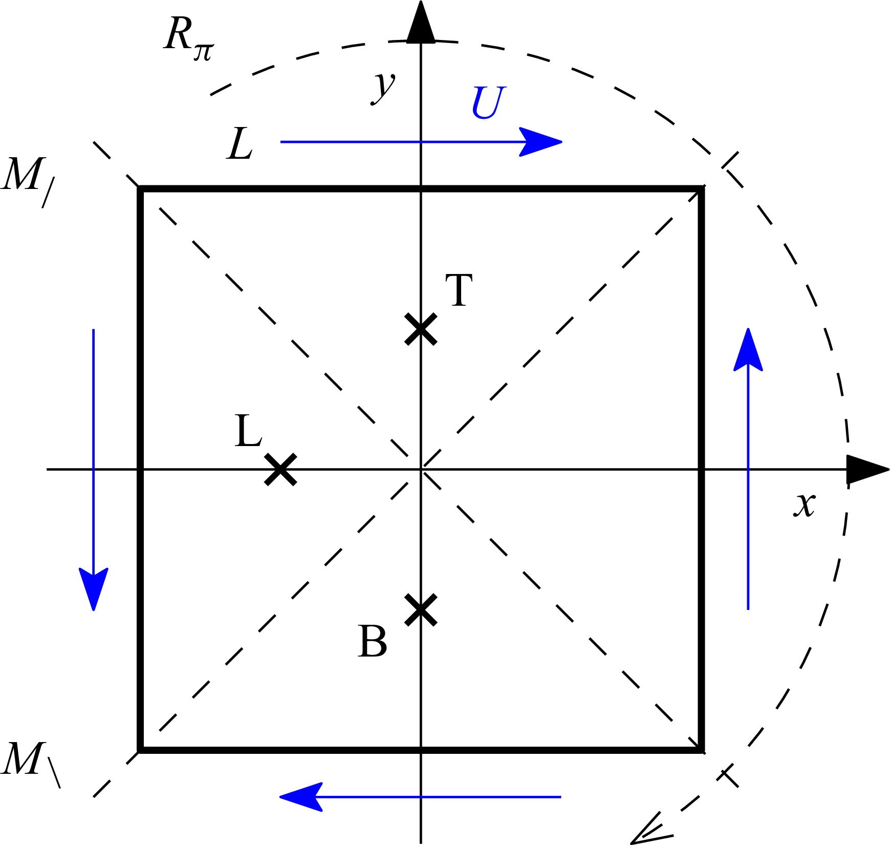


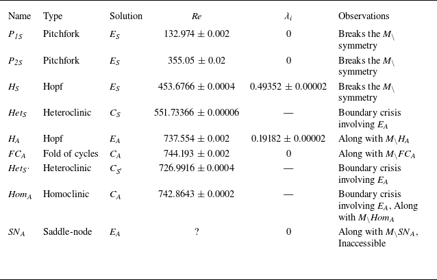


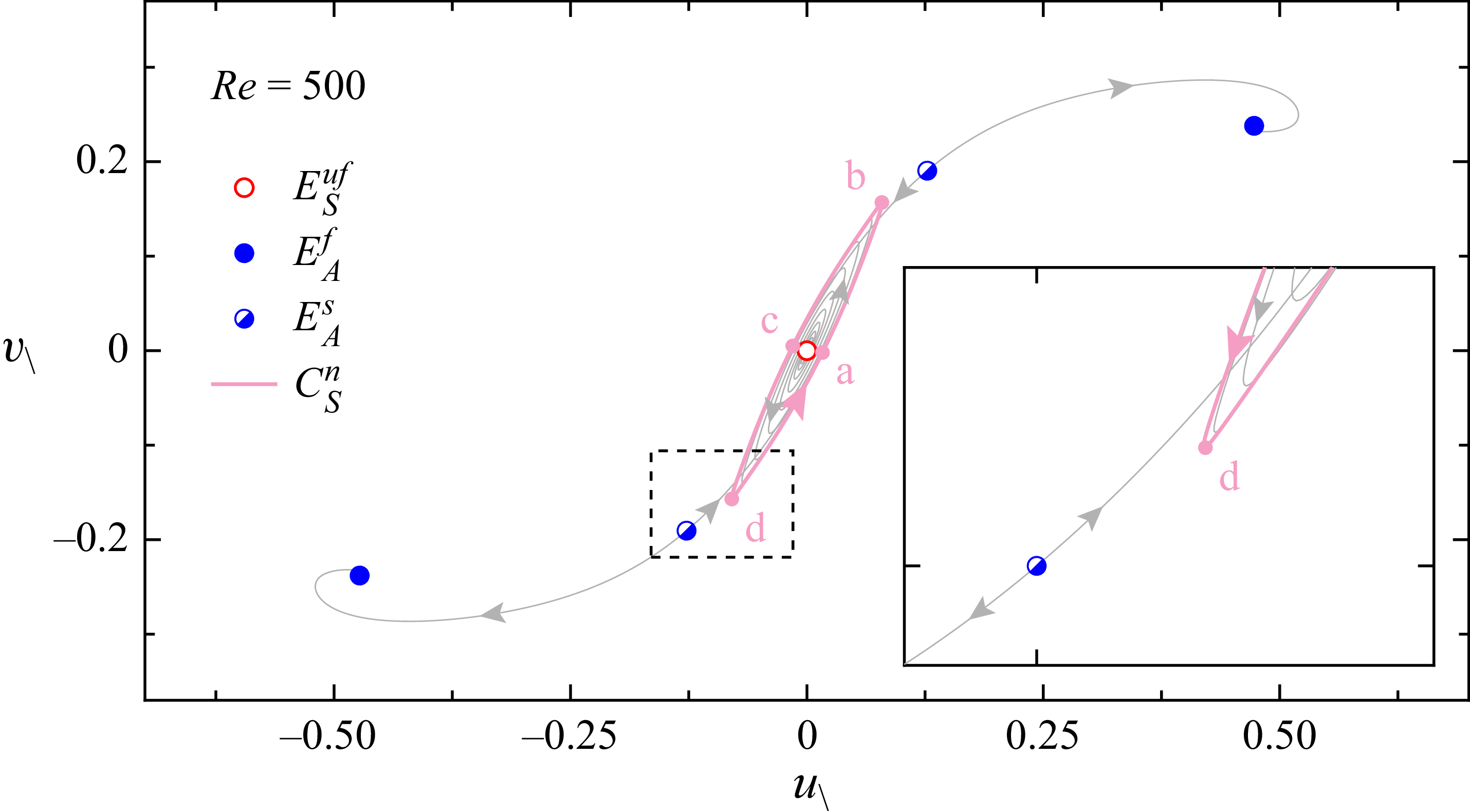


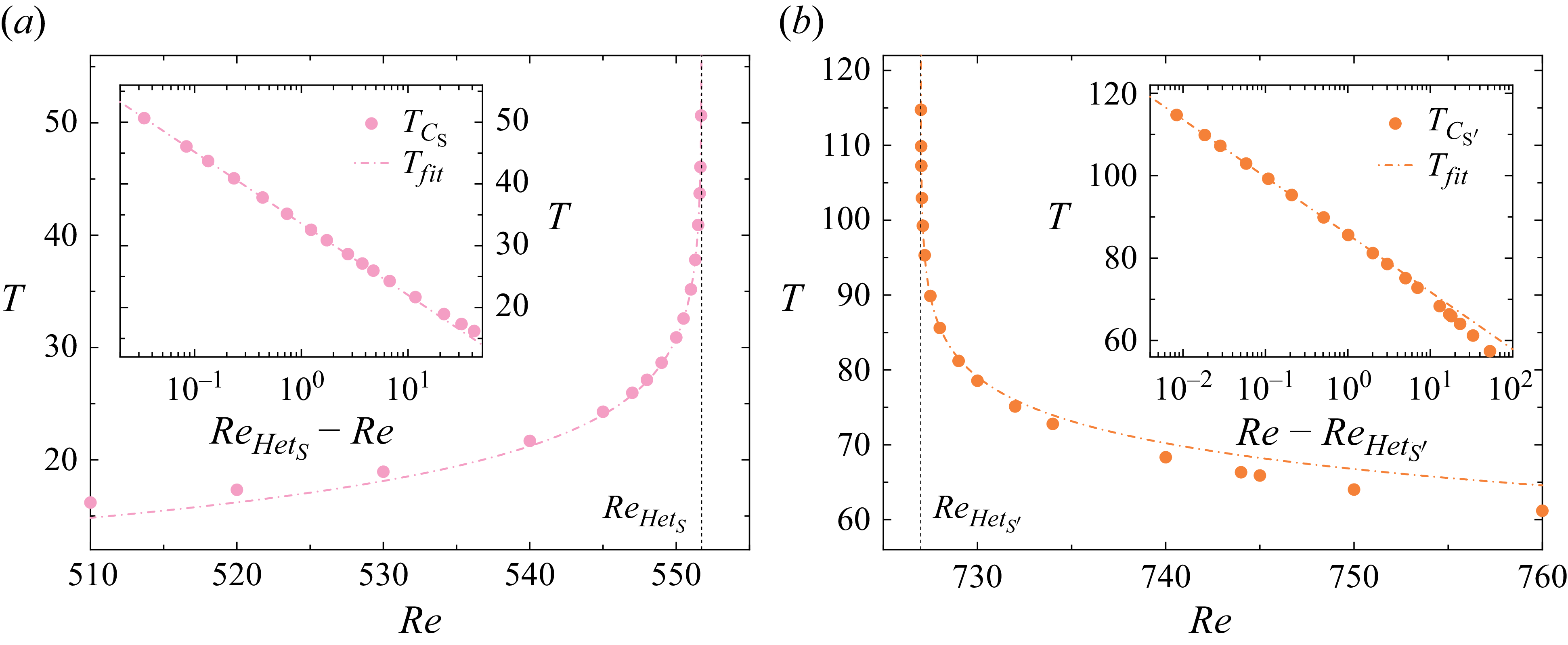


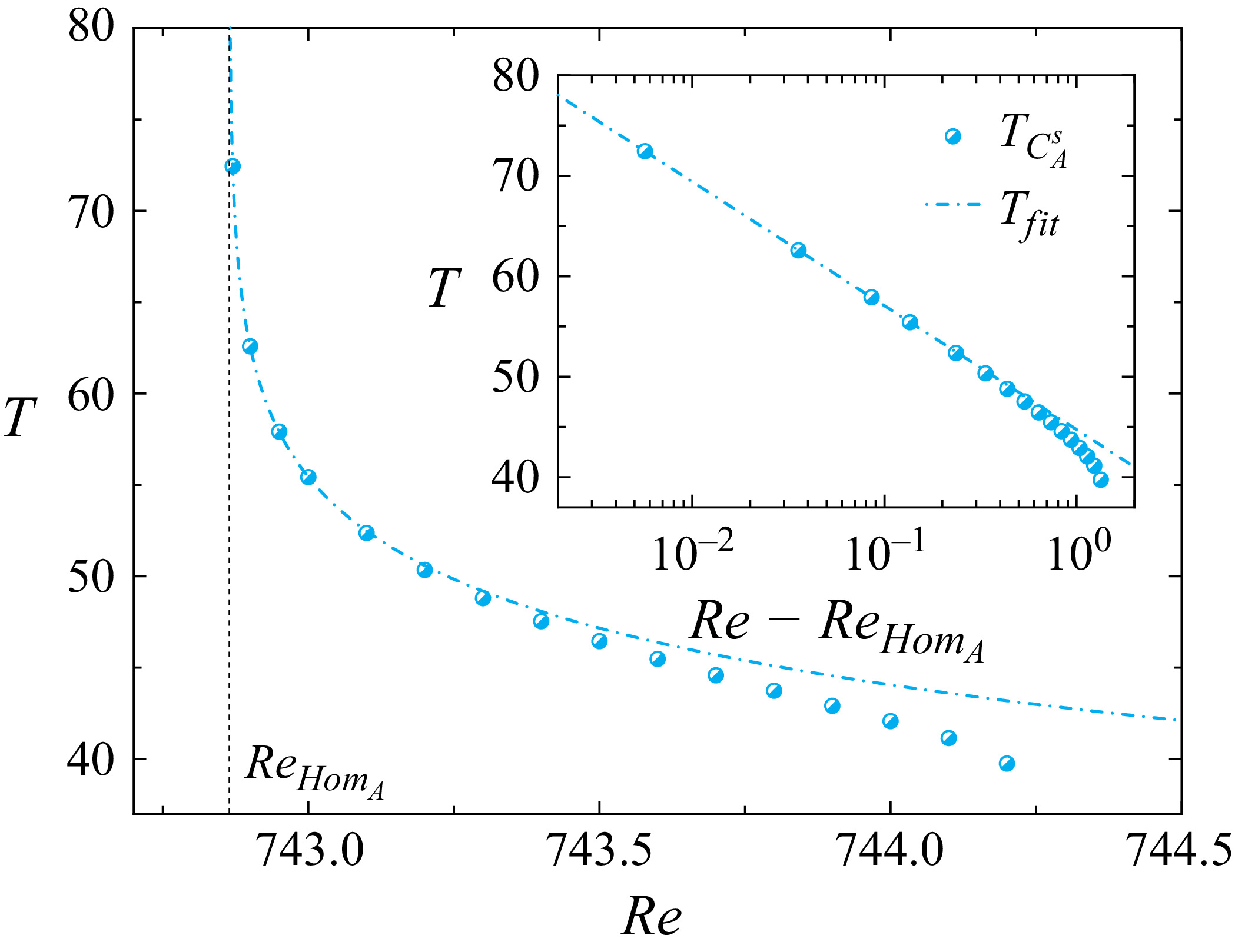


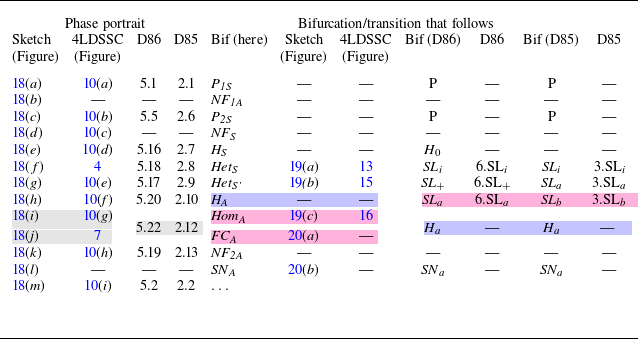


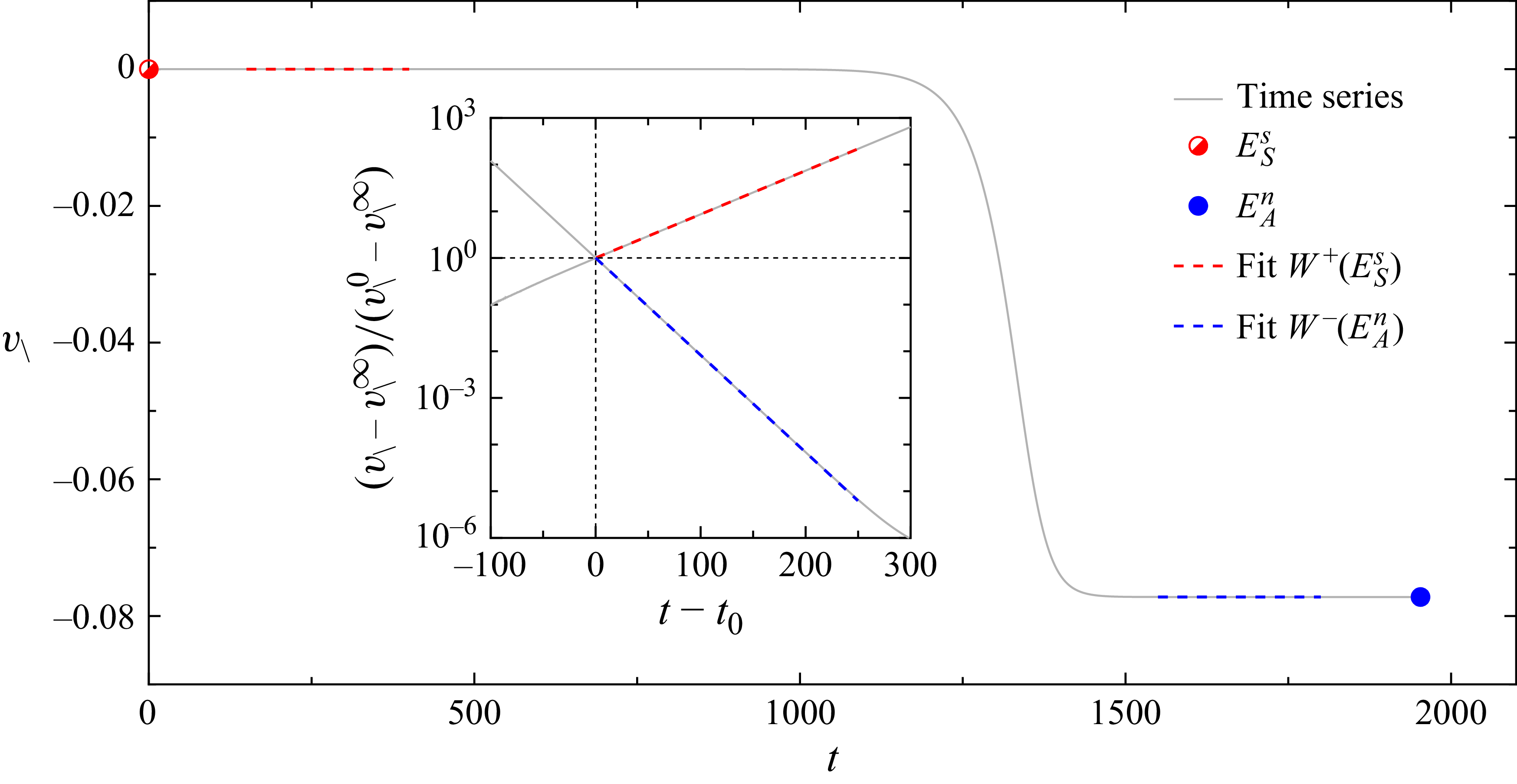


 Open access