


1. Introduction
Magnetic resonance velocimetry (flow-MRI) is an experimental technique that measures fluid velocities in time and three-dimensional space. Flow-MRI is most commonly known for in vivo clinical settings but is gaining popularity within the wider scientific community for in vitro applications (Elkins & Alley Reference Elkins and Alley2007). Whilst flow-MRI can provide reliable velocity measurements, it does not directly provide information about fluid properties such as rheology or pressure. These currently require additional experiments to measure a fluid’s shear-stress–strain curve. Acquiring this non-invasively is challenging as it requires knowledge about both the stress and strain, and some control of either. Common experimental techniques to measure fluid viscosity include rotational and capillary rheometry, which involve passing a fluid sample through a precise geometry and measuring shear rate, torque or pressure drop. Other techniques are available such as industrial ‘in-line’ and ‘on-line’ rheometry, or ultrasound velocity profiling (UVP). However, these methods are either highly invasive (Konigsberg et al. Reference Konigsberg, Nicholson, Halley, Kealy and Bhattacharjee2013) or may require pressure drop measurements (Shwetank et al. Reference Shwetank, Gerhard, Sunil, Asad and Krishna2022). Due to the additional costs and complexities of rheometry experiments, it is not always feasible to acquire rheological data. A non-intrusive in-line UVP rheometry method that does not require pressure drop measurements is presented in Tasaka et al. (Reference Tasaka, Yoshida and Murai2021). More recent techniques include ultrasonic (Ohie et al. Reference Ohie, Yoshida, Tasaka, Sugihara-Seki and Murai2022; Yoshida et al. Reference Yoshida, Ohie and Tasaka2022) and optical (Noto et al. Reference Noto, Ohie, Yoshida and Tasaka2023) spinning rheometry.
For computational fluid dynamic (CFD) simulations of non-Newtonian fluids, rheological behaviour is expressed through viscosity models with adjustable parameters. Model parameters are typically taken from the literature. In biomedical engineering, flow-MRI data can inform patient-specific cardiovascular models. Without patient-specific blood rheology, CFD models lack accuracy. Ranftl et al. (Reference Ranftl, Müller, Windberger, Brenn and von der Linden2023) performed uncertainty quantification to investigate the impact of non-Newtonian and Newtonian CFD models on haemodynamic outputs. They found that patient rheological properties are necessary for accurate wall shear stress predictions, particularly for diseases where blood properties differ from those in healthy populations, and in small arteries where non-Newtonian effects dominate.
Bayesian inference is a data-driven technique that can estimate unknown physical or model parameters and their uncertainties from experimental data combined with some prior knowledge. Worthen et al. (Reference Worthen, Stadler, Petra, Gurnis and Ghattas2014) inferred two unknown parameters of a constitutive equation for viscosity in mantle flow with this approach. The forward problem was governed by a nonlinear Stokes problem and experimental data was of surface velocity measurements. Their method recovered constant and spatially varying parameters reasonably well. Our conceptual approach is similar although the application and technical details differ.
In this study we infer the rheological parameters of a shear-thinning blood analogue from flow-MRI-measured velocity fields alone. We select the Carreau model to represent the non-Newtonian fluid behaviour (Sequeira & Janela Reference Sequeira and Janela2007) because it is differentiable and bounded. Experiments are performed on the US Food and Drug Administration’s (FDA) benchmark nozzle, and data are assimilated using a Bayesian inverse Navier–Stokes (N–S) problem that jointly reconstructs the flow field and learns the Carreau parameters. Our inversion algorithm differs from the aforementioned rheometry methods by inferring rheological properties of non-Newtonian fluids from general velocity fields alone (as long as information on the viscous stress tensor can be retrieved from the field). It relies solely on velocity field measurements, which can be acquired using any velocimetry technique (e.g. flow-MRI, Doppler, or particle image velocimetry). This is the first time flow-MRI has been used for a non-invasive measurement of rheological parameters.
2. Bayesian inversion of the Navier–Stokes problem
We learn the rheology of a non-Newtonian fluid from velocimetry data by solving a Bayesian inverse N–S problem. We first assume that there is a N–S problem with a Carreau fluid model that can explain the velocimetry data, $\boldsymbol {u}^\star$
. Therefore, N–S parameters,
$\boldsymbol {u}^\star$
. Therefore, N–S parameters, $\boldsymbol {x}^\circ$
, exist such that
$\boldsymbol {x}^\circ$
, exist such that
 \begin{gather} \boldsymbol {u}^\star -\mathcal{Z}\boldsymbol {x}^\circ = \boldsymbol {\varepsilon } \sim \mathcal {N}(\boldsymbol {0},\mathcal {C}_{\boldsymbol {u}^\star }), \end{gather}
where $\mathcal {Z}$
is the nonlinear operator that maps N–S parameters to N–S solutions projected into the data space, and
$\mathcal {Z}$
is the nonlinear operator that maps N–S parameters to N–S solutions projected into the data space, and $\boldsymbol {\varepsilon }$
is Gaussian noise with zero mean and covariance operator
$\boldsymbol {\varepsilon }$
is Gaussian noise with zero mean and covariance operator $\mathcal {C}_{\boldsymbol {u}^\star }$
. We do not know
$\mathcal {C}_{\boldsymbol {u}^\star }$
. We do not know $\boldsymbol {x}^\circ$
, but we assume that its prior probability distribution is
$\boldsymbol {x}^\circ$
, but we assume that its prior probability distribution is $\mathcal {N}(\bar {\boldsymbol {x}},\mathcal {C}_{\bar {\boldsymbol {x}}})$
, where
$\mathcal {N}(\bar {\boldsymbol {x}},\mathcal {C}_{\bar {\boldsymbol {x}}})$
, where $\bar {\boldsymbol {x}}$
is the prior mean, and
$\bar {\boldsymbol {x}}$
is the prior mean, and $\mathcal {C}_{\bar {\boldsymbol {x}}}$
is the prior covariance operator. Using Bayes’ theorem we then find that the posterior probability density function (p.d.f.) of
$\mathcal {C}_{\bar {\boldsymbol {x}}}$
is the prior covariance operator. Using Bayes’ theorem we then find that the posterior probability density function (p.d.f.) of $\boldsymbol {x}$
, given the data
$\boldsymbol {x}$
, given the data $\boldsymbol {u}^\star$
, is given by
$\boldsymbol {u}^\star$
, is given by
 \begin{equation} \pi \big (\boldsymbol {x}\big |\boldsymbol {u}^\star \big ) \propto \pi \big (\boldsymbol {u}^\star \big |\boldsymbol {x}\big )\,\pi (\boldsymbol {x}) = \exp \Big (-\tfrac {1}{2}\lVert \boldsymbol {u}^\star -\mathcal {Z}\boldsymbol {x} \rVert ^2_{\mathcal {C}_{\boldsymbol {u}^\star }} - \tfrac {1}{2}\lVert \boldsymbol {x}-\bar {\boldsymbol {x}} \rVert ^2_{\mathcal {C}_{\bar {\boldsymbol {x}}}}\Big ) \quad , \end{equation}
where $\pi (\boldsymbol {u}^\star \big |\boldsymbol {x} )$
is the data likelihood,
$\pi (\boldsymbol {u}^\star \big |\boldsymbol {x} )$
is the data likelihood, $\pi (\boldsymbol {x} )$
is the prior p.d.f. of
$\pi (\boldsymbol {x} )$
is the prior p.d.f. of $\boldsymbol {x}$
, and
$\boldsymbol {x}$
, and $\lVert \cdot ,\cdot \rVert ^2_{\mathcal {C}} := \big \langle \cdot ,\mathcal {C}^{-1}\cdot \big \rangle$
is the covariance-weighted
$\lVert \cdot ,\cdot \rVert ^2_{\mathcal {C}} := \big \langle \cdot ,\mathcal {C}^{-1}\cdot \big \rangle$
is the covariance-weighted $L^2$
-norm. The most likely parameters,
$L^2$
-norm. The most likely parameters, $\boldsymbol {x}^\circ$
, maximise the posterior p.d.f. (maximum a posteriori probability, or MAP estimator), and are given implicitly as the solution of the nonlinear optimisation problem
$\boldsymbol {x}^\circ$
, maximise the posterior p.d.f. (maximum a posteriori probability, or MAP estimator), and are given implicitly as the solution of the nonlinear optimisation problem
 \begin{gather} \quad \boldsymbol {x}^\circ \equiv \underset {\boldsymbol {x}}{\mathrm {argmin}}\mathscr {J}, \quad \text {where}\quad \mathscr {J} := \tfrac {1}{2}\lVert \boldsymbol {u}^\star -\mathcal {Z}\boldsymbol {x} \rVert ^2_{\mathcal {C}_{\boldsymbol {u}^\star }} + \tfrac {1}{2}\lVert \boldsymbol {x}-\bar {\boldsymbol {x}} \rVert ^2_{\mathcal {C}_{\bar {\boldsymbol {x}}}}. \end{gather}
Using a first-order Taylor expansion of $\mathcal {Z}$
around
$\mathcal {Z}$
around $\boldsymbol {x}_k$
, given by
$\boldsymbol {x}_k$
, given by
 \begin{gather} \mathcal {Z}\boldsymbol {x} \simeq \mathcal {Z}\boldsymbol {x}_k + \mathcal {G}_k\,\big (\boldsymbol {x}-\boldsymbol {x}_k \big), \end{gather}
the optimality conditions of problem (2.3) lead to the following iteration (Tarantola Reference Tarantola2005, chap. 6.22.6):
 \begin{gather} \boldsymbol {x}_{k+1} \leftarrow \!\!| \, \boldsymbol {x}_k - \tau _k\,\mathcal {C}_{\boldsymbol {x}_k}\, \big (D_{\boldsymbol {x}}\mathscr {J}\big )_k, \end{gather}
where
 \begin{gather} \big (D_{\boldsymbol {x}}\mathscr {J}\big )_k := -\mathcal {G}_k^*\,\mathcal {C}_{\boldsymbol {u}^\star }^{-1}\big (\boldsymbol {u}^\star -\mathcal {Z}\boldsymbol {x}_k\big ) + \mathcal {C}_{\bar {\boldsymbol {x}}}^{-1}\big (\boldsymbol {x}_k-\bar {\boldsymbol {x}}\big ), \end{gather} $\mathbb {R}\ni \tau _k \gt 0$
is the step size at iteration
$\mathbb {R}\ni \tau _k \gt 0$
is the step size at iteration $k$
, which is determined by a line-search algorithm,
$k$
, which is determined by a line-search algorithm, $\mathcal {G}^{*}_k$
is the adjoint of
$\mathcal {G}^{*}_k$
is the adjoint of $\mathcal {G}_k$
, and
$\mathcal {G}_k$
, and $\mathcal {C}_{\boldsymbol {x}_k}$
is the posterior covariance operator at iteration
$\mathcal {C}_{\boldsymbol {x}_k}$
is the posterior covariance operator at iteration $k$
, which is given by
$k$
, which is given by
 \begin{gather} \mathcal {C}_{\boldsymbol {x}_k} := \big (\mathcal {G}_k^*\,\mathcal {C}_{\boldsymbol {u}^\star }^{-1}\,\mathcal {G}_k+\mathcal {C}_{\bar {\boldsymbol {x}}}^{-1}\big )^{-1}. \end{gather}
The posterior covariance operator around the MAP estimate, $\mathcal {C}_{\boldsymbol {x}^\circ }$
, can then be used to approximate the posterior p.d.f. such that
$\mathcal {C}_{\boldsymbol {x}^\circ }$
, can then be used to approximate the posterior p.d.f. such that
 \begin{equation} \pi \big (\boldsymbol {x}\big |\boldsymbol {u}^\star \big )\simeq \exp \Big ({-}\tfrac {1}{2}\lVert \boldsymbol {x}-\boldsymbol {x}^\circ \rVert ^2_{\mathcal {C}_{\boldsymbol {x}^\circ }} - \textrm {const.}\Big ), \end{equation}
which is known as the Laplace approximation (MacKay Reference MacKay2003, chap. 27). For linear models, the approximation is exact when both $\pi (\boldsymbol {u}^\star \big |\boldsymbol {x} )$
and
$\pi (\boldsymbol {u}^\star \big |\boldsymbol {x} )$
and $\pi (\boldsymbol {x})$
are normal. For nonlinear models, the accuracy of the approximation depends on the behaviour of the operator
$\pi (\boldsymbol {x})$
are normal. For nonlinear models, the accuracy of the approximation depends on the behaviour of the operator $\mathcal {Z}$
around the critical point
$\mathcal {Z}$
around the critical point $\boldsymbol {x}^\circ$
(Kontogiannis et al. Reference Kontogiannis, Elgersma, Sederman and Juniper2024a
, § 2.2).
$\boldsymbol {x}^\circ$
(Kontogiannis et al. Reference Kontogiannis, Elgersma, Sederman and Juniper2024a
, § 2.2).
2.1. The N–S problem and the operators $\mathcal {Z}$
,
$\mathcal {G}$
$\mathcal {Z}$
,
$\mathcal {G}$


In order to solve the inverse problem (2.3) using (2.5)–(2.7), we need to define $\mathcal {Z}$
and
$\mathcal {Z}$
and $\mathcal {G}$
. We start from the N–S boundary value problem in
$\mathcal {G}$
. We start from the N–S boundary value problem in $\Omega \subset \mathbb {R}^3$
:
$\Omega \subset \mathbb {R}^3$
:
 \begin{gather} \boldsymbol {u}\boldsymbol {\cdot }\nabla \boldsymbol {u}-\nabla \boldsymbol {\cdot }\big (2\nu _e\nabla ^s\boldsymbol {u}\big ) + \nabla p = \boldsymbol {0} \quad \text {and}\quad \nabla \boldsymbol {\cdot } \boldsymbol {u} = 0 \quad \textrm {in}\quad \Omega,\nonumber \\ \boldsymbol {u} = \boldsymbol {0} \quad \textrm {on}\quad \Gamma,\quad \boldsymbol {u} = \boldsymbol {g}_i \quad \textrm {on}\quad \Gamma _i,\quad -2\nu _e\nabla ^s\boldsymbol {u}\boldsymbol {\cdot }\boldsymbol {\nu }+p\boldsymbol {\nu } = \boldsymbol {g}_o \quad \textrm {on} \quad \Gamma _o, \end{gather}
where $\boldsymbol {u}$
is the velocity,
$\boldsymbol {u}$
is the velocity, $p\leftarrow \!| p/\rho$
is the reduced pressure,
$p\leftarrow \!| p/\rho$
is the reduced pressure, $\rho$
is the density,
$\rho$
is the density, $\nu _e$
is the effective kinematic viscosity,
$\nu _e$
is the effective kinematic viscosity, $(\nabla ^s \boldsymbol {u})_{ij} := ({1}/{2})(\partial _j u_i + \partial _i u_j)$
is the strain-rate tensor,
$(\nabla ^s \boldsymbol {u})_{ij} := ({1}/{2})(\partial _j u_i + \partial _i u_j)$
is the strain-rate tensor, $\boldsymbol {g}_i$
is the Dirichlet boundary condition (b.c.) at the inlet
$\boldsymbol {g}_i$
is the Dirichlet boundary condition (b.c.) at the inlet $\Gamma _i$
,
$\Gamma _i$
, $\boldsymbol {g}_o$
is the natural b.c. at the outlet
$\boldsymbol {g}_o$
is the natural b.c. at the outlet $\Gamma _o$
, and
$\Gamma _o$
, and $\boldsymbol {\nu }$
is the unit normal vector on the boundary
$\boldsymbol {\nu }$
is the unit normal vector on the boundary $\partial \Omega = \Gamma \cup \Gamma _i\cup \Gamma _o$
, where
$\partial \Omega = \Gamma \cup \Gamma _i\cup \Gamma _o$
, where $\Gamma$
is the no-slip boundary (wall). The construction of the operators
$\Gamma$
is the no-slip boundary (wall). The construction of the operators $\mathcal {Z}, \mathcal {G}$
of the generalised inverse N–S problem, whose unknown parameters are the shape of the domain
$\mathcal {Z}, \mathcal {G}$
of the generalised inverse N–S problem, whose unknown parameters are the shape of the domain $\Omega$
, the boundary conditions
$\Omega$
, the boundary conditions $\boldsymbol {g}_i, \boldsymbol {g}_o$
, and the viscosity field
$\boldsymbol {g}_i, \boldsymbol {g}_o$
, and the viscosity field $\nu _e$
, is treated in Kontogiannis et al. (Reference Kontogiannis, Elgersma, Sederman and Juniper2022); Kontogiannis & Juniper (Reference Kontogiannis and Juniper2023); Kontogiannis et al. (Reference Kontogiannis, Elgersma, Sederman and Juniper2024a
). Here, we fix the geometry,
$\nu _e$
, is treated in Kontogiannis et al. (Reference Kontogiannis, Elgersma, Sederman and Juniper2022); Kontogiannis & Juniper (Reference Kontogiannis and Juniper2023); Kontogiannis et al. (Reference Kontogiannis, Elgersma, Sederman and Juniper2024a
). Here, we fix the geometry, $\Omega$
, and the outlet b.c.,
$\Omega$
, and the outlet b.c., $\boldsymbol {g}_o$
, and infer only the inlet b.c.,
$\boldsymbol {g}_o$
, and infer only the inlet b.c., $\boldsymbol {g}_i$
, and the effective viscosity field,
$\boldsymbol {g}_i$
, and the effective viscosity field, $\nu _e$
. We further introduce the Carreau model for the effective viscosity field, which is given by
$\nu _e$
. We further introduce the Carreau model for the effective viscosity field, which is given by
 \begin{align} \mu _e(\dot {\gamma };\boldsymbol {p}_\mu ) &:= \mu _\infty + \delta \mu \big (1 +(\lambda \dot {\gamma })^2\big )^{({n}-1)/{2}}, \end{align}
where $\mu _e := \nu _e\rho$
,
$\mu _e := \nu _e\rho$
, $\dot {\gamma }(\boldsymbol {u}) := \sqrt {2\nabla ^s\boldsymbol {u}\boldsymbol {:}\nabla ^s\boldsymbol {u}}$
is the magnitude of the strain-rate tensor, and
$\dot {\gamma }(\boldsymbol {u}) := \sqrt {2\nabla ^s\boldsymbol {u}\boldsymbol {:}\nabla ^s\boldsymbol {u}}$
is the magnitude of the strain-rate tensor, and $\boldsymbol {p}_\mu := (\mu _\infty ,\delta \mu ,\lambda ,n )$
are the Carreau fluid parameters. In order to infer the most likely viscosity field,
$\boldsymbol {p}_\mu := (\mu _\infty ,\delta \mu ,\lambda ,n )$
are the Carreau fluid parameters. In order to infer the most likely viscosity field, $\mu ^\circ _e$
, we therefore need to infer the most likely Carreau fluid parameters,
$\mu ^\circ _e$
, we therefore need to infer the most likely Carreau fluid parameters, $\boldsymbol {p}^\circ _\mu$
.
$\boldsymbol {p}^\circ _\mu$
.
After linearising problem (2.9) around $\boldsymbol {u}_k$
, we obtain
$\boldsymbol {u}_k$
, we obtain $\boldsymbol {u}(\boldsymbol {x}) \simeq \boldsymbol {u}_k + \mathcal {A}_k (\boldsymbol {x}-\boldsymbol {x}_k)$
, where
$\boldsymbol {u}(\boldsymbol {x}) \simeq \boldsymbol {u}_k + \mathcal {A}_k (\boldsymbol {x}-\boldsymbol {x}_k)$
, where $\mathcal {A}_k \equiv ((D^{\mathscr {M}}_{\boldsymbol {u}})^{-1}D^{\mathscr {M}}_{\boldsymbol {x}} )_k$
, with
$\mathcal {A}_k \equiv ((D^{\mathscr {M}}_{\boldsymbol {u}})^{-1}D^{\mathscr {M}}_{\boldsymbol {x}} )_k$
, with $\mathcal {A}_k$
being a linear, invertible operator, which encapsulates the inverse Jacobian of the N–S problem,
$\mathcal {A}_k$
being a linear, invertible operator, which encapsulates the inverse Jacobian of the N–S problem, $(D^{\mathscr {M}}_{\boldsymbol {u}})^{-1}$
, and the generalised gradient of the velocity field with respect to the parameters
$(D^{\mathscr {M}}_{\boldsymbol {u}})^{-1}$
, and the generalised gradient of the velocity field with respect to the parameters $\boldsymbol {x}$
,
$\boldsymbol {x}$
, $D^{\mathscr {M}}_{\boldsymbol {x}}$
. Observing that
$D^{\mathscr {M}}_{\boldsymbol {x}}$
. Observing that $\mathcal {Z}, \mathcal {G}$
map from the N–S parameter space to the (velocimetry) data space, we define
$\mathcal {Z}, \mathcal {G}$
map from the N–S parameter space to the (velocimetry) data space, we define $\mathcal {Z} := \mathcal {S}\mathcal {Q}$
and
$\mathcal {Z} := \mathcal {S}\mathcal {Q}$
and $\mathcal {G}_k := \mathcal {S}\mathcal {A}_k$
, where
$\mathcal {G}_k := \mathcal {S}\mathcal {A}_k$
, where $\mathcal {S}:\boldsymbol {M}\to \boldsymbol {D}$
is a projection from the model space,
$\mathcal {S}:\boldsymbol {M}\to \boldsymbol {D}$
is a projection from the model space, $\boldsymbol {M}$
, to the data space,
$\boldsymbol {M}$
, to the data space, $\boldsymbol {D}$
, and
$\boldsymbol {D}$
, and $\mathcal {Q}$
is the operator that maps
$\mathcal {Q}$
is the operator that maps $\boldsymbol {x}$
to
$\boldsymbol {x}$
to $\boldsymbol {u}$
, i.e. that solves the N–S problem. (The operators
$\boldsymbol {u}$
, i.e. that solves the N–S problem. (The operators $\mathcal {S},\mathcal {Q},\mathcal {A}$
are derived in Kontogiannis et al. (Reference Kontogiannis, Elgersma, Sederman and Juniper2024a) from the weak form of the N–S problem (2.9),
$\mathcal {S},\mathcal {Q},\mathcal {A}$
are derived in Kontogiannis et al. (Reference Kontogiannis, Elgersma, Sederman and Juniper2024a) from the weak form of the N–S problem (2.9), $\mathscr {M}$
.)
$\mathscr {M}$
.)
Based on the above definitions, and due to (2.6), we observe that the model contribution to the objective’s steepest descent direction, for the Carreau parameters, $\boldsymbol {p}_\mu$
, is
$\boldsymbol {p}_\mu$
, is
 \begin{gather} \big (\delta \boldsymbol {p}_{\mu }\big )_k := \mathcal {G}_k^*\,\mathcal {C}_{\boldsymbol {u}^\star }^{-1}\big (\boldsymbol {u}^\star -\mathcal {Z}\boldsymbol {x}_k\big ) = \underbrace {\big (D^{\mathscr {M}}_{\boldsymbol {p}_{\mu }}\big )^*_k\, \big ((D^{\mathscr {M}}_{\boldsymbol {u}})^{*}\big )^{-1}_k}_{D^{\boldsymbol {p}_{\mu }}_{\boldsymbol {u}}}\,\underbrace {\mathcal {S}^*\,\mathcal {C}_{\boldsymbol {u}^\star }^{-1}\big (\boldsymbol {u}^\star -\mathcal {S}\boldsymbol {u}_k\big )}_{\text {data-model discrepancy } \delta \boldsymbol {u} \in \boldsymbol {M}}. \end{gather}
Even though $D^{\mathscr {M}}_{\boldsymbol {u}}$
is invertible, for large-scale problems (such as those in fluid dynamics) its inverse,
$D^{\mathscr {M}}_{\boldsymbol {u}}$
is invertible, for large-scale problems (such as those in fluid dynamics) its inverse, $(D^{\mathscr {M}}_{\boldsymbol {u}})^{-1}$
, cannot be stored in computer memory because its discrete form produces a dense matrix. The discrete form of
$(D^{\mathscr {M}}_{\boldsymbol {u}})^{-1}$
, cannot be stored in computer memory because its discrete form produces a dense matrix. The discrete form of $D^{\mathscr {M}}_{\boldsymbol {u}}$
, however, produces a sparse matrix. Consequently, instead of using the explicit formula (2.11), the steepest descent directions are given by
$D^{\mathscr {M}}_{\boldsymbol {u}}$
, however, produces a sparse matrix. Consequently, instead of using the explicit formula (2.11), the steepest descent directions are given by
 \begin{gather} \big (\delta \boldsymbol {p}_{\mu }\big )_k := \big (D^{\mathscr {M}}_{\boldsymbol {p}_{\mu }}\big )^*_k\,\boldsymbol {v}_k = 2\int _\Omega \big (D_{\boldsymbol {p}_\mu }\mu _e\big )_k\big (\nabla ^s\boldsymbol {u}_k\boldsymbol {:}\nabla ^s\boldsymbol {v}_k\big ), \end{gather}
where ${ (D_{\boldsymbol {p}_\mu }\mu _e )}_k \equiv D_{\boldsymbol {p}_\mu }\mu _e (\dot {\gamma }(\boldsymbol {u}_k);(\boldsymbol {p}_{\mu })_k )$
consists of the derivatives of the Carreau model with respect to its parameters, and
${ (D_{\boldsymbol {p}_\mu }\mu _e )}_k \equiv D_{\boldsymbol {p}_\mu }\mu _e (\dot {\gamma }(\boldsymbol {u}_k);(\boldsymbol {p}_{\mu })_k )$
consists of the derivatives of the Carreau model with respect to its parameters, and $\boldsymbol {v}_k$
is the adjoint velocity field, which is obtained by solving the following linear operator equation:
$\boldsymbol {v}_k$
is the adjoint velocity field, which is obtained by solving the following linear operator equation:
 \begin{gather} A\boldsymbol {v}_k = b,\quad \text {where}\quad A \equiv \big (D^{\mathscr {M}}_{\boldsymbol {u}}\big )_k^*\quad \text {and}\quad b \equiv \mathcal {S}^*\mathcal {C}_{\boldsymbol {u}^\star }^{-1}\big (\boldsymbol {u}^\star -\mathcal {S}\boldsymbol {u}_k\big ). \end{gather}
The steepest descent directions for the inlet b.c., $\boldsymbol {g}_i$
, are derived in Kontogiannis et al. (Reference Kontogiannis, Elgersma, Sederman and Juniper2024a
).
$\boldsymbol {g}_i$
, are derived in Kontogiannis et al. (Reference Kontogiannis, Elgersma, Sederman and Juniper2024a
).
Instead of explicitly computing $\mathcal {C}_{\boldsymbol {x}_k}$
at every iteration using (2.7), we approximate
$\mathcal {C}_{\boldsymbol {x}_k}$
at every iteration using (2.7), we approximate $\mathcal {C}_{\boldsymbol {x}_k}$
using the damped Broyden–Fletcher–Goldfarb–Shanno (BFGS) quasi-Newton method (Goldfarb et al. Reference Goldfarb, Ren, Bahamou, Larochelle, Ranzato, Hadsell, Balcan and Lin2020), which ensures that
$\mathcal {C}_{\boldsymbol {x}_k}$
using the damped Broyden–Fletcher–Goldfarb–Shanno (BFGS) quasi-Newton method (Goldfarb et al. Reference Goldfarb, Ren, Bahamou, Larochelle, Ranzato, Hadsell, Balcan and Lin2020), which ensures that $\mathcal {C}_{\boldsymbol {x}_k}$
remains positive definite, and its approximation remains numerically stable.
$\mathcal {C}_{\boldsymbol {x}_k}$
remains positive definite, and its approximation remains numerically stable.
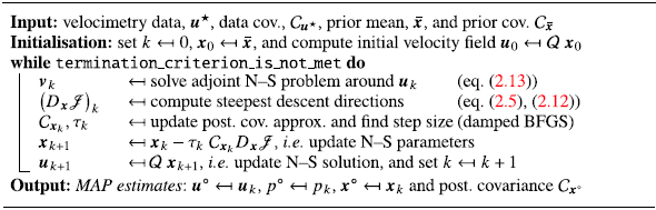
Learning rheological parameters from velocimetry data.
2.1.1. Note on effective viscosity model selection
In this study, although we fix the effective viscosity model to the Carreau fluid model, which is given by (2.10), the present Bayesian inversion framework is already set up for model selection (Yoko & Juniper Reference Yoko and Juniper2024a
, § 4.3). The velocimetry data, $\boldsymbol {u}^\star$
, can be assimilated into the N–S boundary value problem with as many different viscosity models as the user likes. The model parameter uncertainties are then estimated, and the marginal likelihood of each model is calculated. The marginal likelihood is the likelihood of each model, given the experimental data, which is also known as the evidence for each model. The models are then ranked by their evidence, and the most accurate model is chosen. Bayesian rheological model ranking using rheometry data has been addressed in Freund & Ewoldt (Reference Freund and Ewoldt2015). Note that, here we infer the rheology of the fluid from velocimetry data (instead of rheometry data), which is a more difficult problem. Bayesian rheological model ranking from velocimetry data are a natural extension of the present Bayesian inversion framework, and provides scope for future work. (Another extension that follows naturally is optimal experiment design (Yoko & Juniper Reference Yoko and Juniper2024b
, § 4.3, § 4.1), i.e. strategically planning experiments to maximise information gain in parameter estimation.)
$\boldsymbol {u}^\star$
, can be assimilated into the N–S boundary value problem with as many different viscosity models as the user likes. The model parameter uncertainties are then estimated, and the marginal likelihood of each model is calculated. The marginal likelihood is the likelihood of each model, given the experimental data, which is also known as the evidence for each model. The models are then ranked by their evidence, and the most accurate model is chosen. Bayesian rheological model ranking using rheometry data has been addressed in Freund & Ewoldt (Reference Freund and Ewoldt2015). Note that, here we infer the rheology of the fluid from velocimetry data (instead of rheometry data), which is a more difficult problem. Bayesian rheological model ranking from velocimetry data are a natural extension of the present Bayesian inversion framework, and provides scope for future work. (Another extension that follows naturally is optimal experiment design (Yoko & Juniper Reference Yoko and Juniper2024b
, § 4.3, § 4.1), i.e. strategically planning experiments to maximise information gain in parameter estimation.)
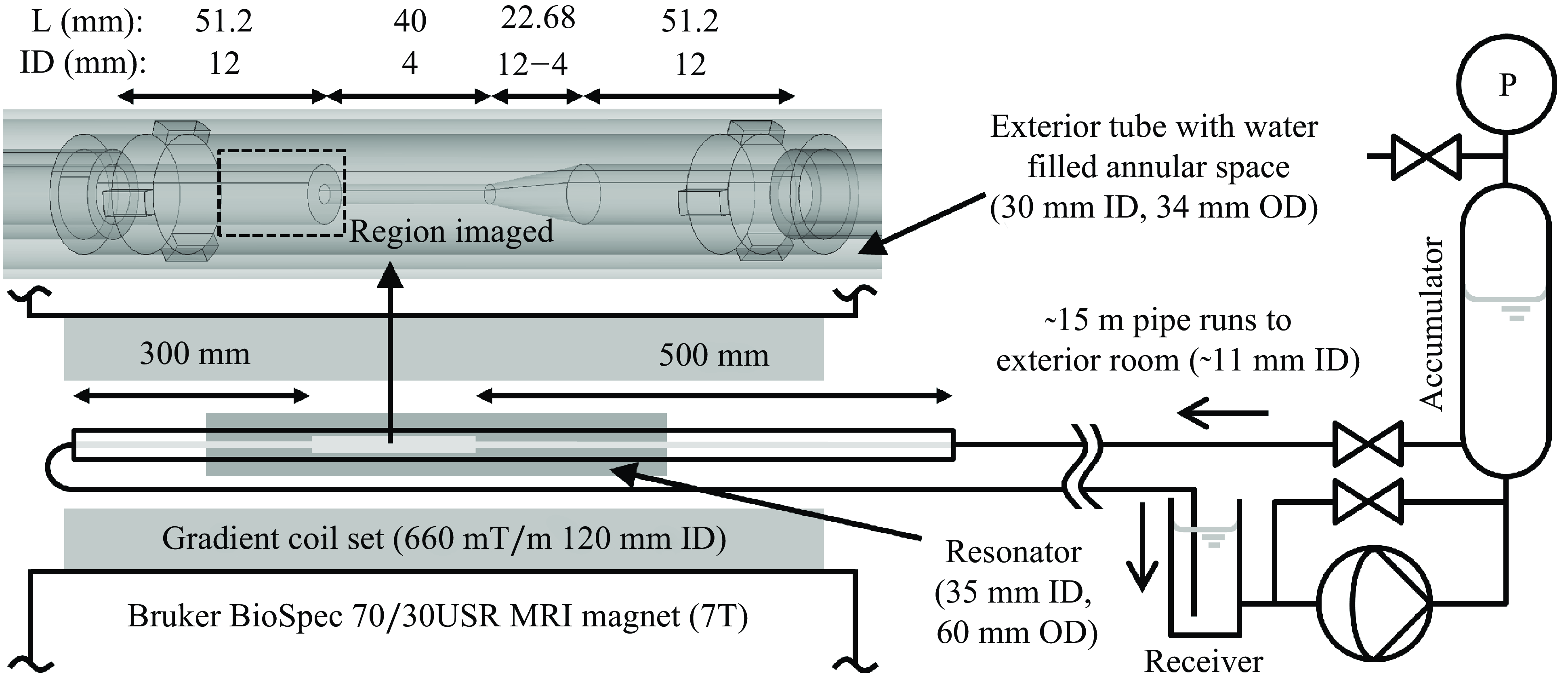
Overall flow system and set-up around the MRI scanner with detail of the FDA flow nozzle geometry implemented: ID, inner diameter; OD, outer diameter.
3. Flow-MRI experiment of a non-Newtonian laminar jet
The test section is part of the FDA nozzle (Hariharan et al. Reference Hariharan2011; Stewart et al. Reference Stewart2012), which is an axisymmetric pipe that converges to a narrow throat section, followed by a sudden expansion, where a non-Newtonian laminar jet forms (see figure 1). The geometry was three-dimensionally (3-D) resin-printed to a nominal tolerance of $\pm$
0.2 mm. Acrylic tubes were attached upstream and downstream of the test section, and the former was equipped with a flow straightener array. The test section was placed inside a water-filled acrylic outer tube in order to avoid air-induced magnetic susceptibility gradients. A pipe loop provided flow from pumping hardware outside the MRI scanner room, with the return pipe looping back through an annular gap between the resonator body and the gradient coil inner diameter. Flow was collected in a receiver reservoir, pumped via a variable speed diaphragm pump, fed to a pulsation dampening accumulator, and then back to the test section. Controlled pump bypass enabled very low flow rates whilst keeping the pump oscillation frequency high. Loop circulation time scales are of the order of the scanning time scale. The flow loop was purged of bubbles after filling, and K-Type and alcohol thermometer measurements indicated a fluid (ambient) temperature of 21.8 ∘C.
$\pm$
0.2 mm. Acrylic tubes were attached upstream and downstream of the test section, and the former was equipped with a flow straightener array. The test section was placed inside a water-filled acrylic outer tube in order to avoid air-induced magnetic susceptibility gradients. A pipe loop provided flow from pumping hardware outside the MRI scanner room, with the return pipe looping back through an annular gap between the resonator body and the gradient coil inner diameter. Flow was collected in a receiver reservoir, pumped via a variable speed diaphragm pump, fed to a pulsation dampening accumulator, and then back to the test section. Controlled pump bypass enabled very low flow rates whilst keeping the pump oscillation frequency high. Loop circulation time scales are of the order of the scanning time scale. The flow loop was purged of bubbles after filling, and K-Type and alcohol thermometer measurements indicated a fluid (ambient) temperature of 21.8 ∘C.
The test solution used here is a 46 wt % haematocrit level blood analogue (Brookshier & Tarbell Reference Brookshier and Tarbell1993) (0.5 wt % NaCl was omitted because it would interfere with MRI). A 40 wt % glycerine solution in deionised water was first prepared and then used as the solvent for a 0.04 wt % xantham gum solution. The solution appears weakly viscoelastic, with viscous stresses above elastic stresses in their 2 Hz oscillatory shear tests, justifying the generalised Newtonian fluid assumption.
Flow-MRI was performed using a Bruker BioSpec 70/30USR 7T preclinical scanner (660 mT/m gradients, 35 mm ID resonator coil). Images were acquired with uniform radial pixel spacing of 0.1 mm and axial slice thickness of 0.08 mm. Four scan repetitions were performed in order to reduce noise ( $\sim$
15 min total scanning time).
$\sim$
15 min total scanning time).
3.1. Flow-MRI data preprocessing
We use phase-contrast MRI and Hadamard encoding to measure all three components of a 3-D velocity field using a single set of four, fully sampled $\boldsymbol {k}$
-space scans,
$\boldsymbol {k}$
-space scans, $\{{s}\}_{j=1}^4$
. For each scan we compute its respective complex image,
$\{{s}\}_{j=1}^4$
. For each scan we compute its respective complex image, $w_j$
, which is given by
$w_j$
, which is given by
 \begin{gather} w_j := \rho _j e^{i\varphi _j} = \mathcal {F}^{-1}s_j, \end{gather}
where $\rho _j$
is the nuclear spin density image,
$\rho _j$
is the nuclear spin density image, $\varphi _j$
is the phase image and
$\varphi _j$
is the phase image and $\mathcal {F}$
is the Fourier transform. The velocity components
$\mathcal {F}$
is the Fourier transform. The velocity components $u_i$
, for
$u_i$
, for $i=1,\dots, 3$
, are then given by
$i=1,\dots, 3$
, are then given by
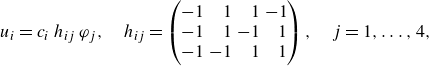 \begin{gather} u_i = c_i\,h_{ij}\,\varphi _j,\quad h_{ij}= \begin{pmatrix} -1 & \hphantom {-}1 & \hphantom {-}1 & -1\\ -1 & \hphantom {-}1 & -1 & \hphantom {-}1\\ -1 & -1 & \hphantom {-}1 & \hphantom {-}1 \end{pmatrix},\quad j=1,\ldots, 4, \end{gather}
where repeated indices imply summation, and $c_i$
is a known constant that depends on the gyromagnetic ratio of hydrogen and the gradient pulse properties. In order to remove any phase shift contributions that are not caused by the flow, we conduct an additional no-flow experiment. That is, we acquire a set of four
$c_i$
is a known constant that depends on the gyromagnetic ratio of hydrogen and the gradient pulse properties. In order to remove any phase shift contributions that are not caused by the flow, we conduct an additional no-flow experiment. That is, we acquire a set of four $\boldsymbol {k}$
-space scans,
$\boldsymbol {k}$
-space scans, $\{\bar {s}\}_{j=1}^4$
, for the same geometry and field-of-view, but with zero flow (stagnant fluid). We then obtain the no-flow complex images,
$\{\bar {s}\}_{j=1}^4$
, for the same geometry and field-of-view, but with zero flow (stagnant fluid). We then obtain the no-flow complex images, $\bar {w}_j$
, using (3.1), and compute the corresponding no-flow velocity images using (3.2), such that
$\bar {w}_j$
, using (3.1), and compute the corresponding no-flow velocity images using (3.2), such that $\bar {u}_i = \bar {c}_i h_{ij} \bar {\varphi }_j$
, where
$\bar {u}_i = \bar {c}_i h_{ij} \bar {\varphi }_j$
, where $\bar {c}_i$
is the no-flow constant, which is known. The corrected velocity is then given by
$\bar {c}_i$
is the no-flow constant, which is known. The corrected velocity is then given by $u_i = c_i\theta (h_{ij}\varphi _j) - \bar {c}_i\theta (h_{ij}\bar {\varphi }_j)$
, where
$u_i = c_i\theta (h_{ij}\varphi _j) - \bar {c}_i\theta (h_{ij}\bar {\varphi }_j)$
, where $\theta (x) := x - 2\pi (\lfloor (\lfloor {x}/\pi \rfloor -1)/2\rfloor + 1)$
is the phase difference unwrapping function, and
$\theta (x) := x - 2\pi (\lfloor (\lfloor {x}/\pi \rfloor -1)/2\rfloor + 1)$
is the phase difference unwrapping function, and $\lfloor {\cdot }/\cdot \rfloor$
denotes integer division. To increase the signal-to-noise ratio (SNR) of steady flow images we acquire
$\lfloor {\cdot }/\cdot \rfloor$
denotes integer division. To increase the signal-to-noise ratio (SNR) of steady flow images we acquire $n$
sets (in this study
$n$
sets (in this study $n=4$
) of
$n=4$
) of $\boldsymbol {k}$
-space scans, generate their respective velocity images
$\boldsymbol {k}$
-space scans, generate their respective velocity images $\{u_i\}_{k=1}^{n}$
, and compute the average velocity image
$\{u_i\}_{k=1}^{n}$
, and compute the average velocity image $\sum _{k=1}^{n} (u_i)_k/n$
. The noise variance in the averaged velocity images then reduces to
$\sum _{k=1}^{n} (u_i)_k/n$
. The noise variance in the averaged velocity images then reduces to $\sigma ^2/n$
, where
$\sigma ^2/n$
, where $\sigma ^2$
is the noise variance of each individual velocity image. We straighten and centre the averaged flow-MRI images, and, since the flow is axisymmetric, we mirror-average the images to further increase SNR and enforce mirror-symmetry. We generate a mask for the region of interest by segmenting the mirror-averaged nuclear spin density image, and apply this mask to the velocity images. Because we solve an inverse N–S problem in a 3-D discrete space comprising trilinear finite elements (voxels), the final preprocessing step is to
$\sigma ^2$
is the noise variance of each individual velocity image. We straighten and centre the averaged flow-MRI images, and, since the flow is axisymmetric, we mirror-average the images to further increase SNR and enforce mirror-symmetry. We generate a mask for the region of interest by segmenting the mirror-averaged nuclear spin density image, and apply this mask to the velocity images. Because we solve an inverse N–S problem in a 3-D discrete space comprising trilinear finite elements (voxels), the final preprocessing step is to $L^2$
-project the two-dimensional (2-D) axisymmetric flow-MRI images,
$L^2$
-project the two-dimensional (2-D) axisymmetric flow-MRI images, $(u_r,u_z)$
, to their corresponding 3-D flow field,
$(u_r,u_z)$
, to their corresponding 3-D flow field, $\boldsymbol {u}^\star =(u^\star _x,u^\star _y,u^\star _z)$
. Note that the 3-D data that we generate (Kontogiannis et al. Reference Kontogiannis, Hodgkinson, Reynolds and Manchester2024b
) have the same (2-D) spatial resolution as the 2-D images.
$\boldsymbol {u}^\star =(u^\star _x,u^\star _y,u^\star _z)$
. Note that the 3-D data that we generate (Kontogiannis et al. Reference Kontogiannis, Hodgkinson, Reynolds and Manchester2024b
) have the same (2-D) spatial resolution as the 2-D images.
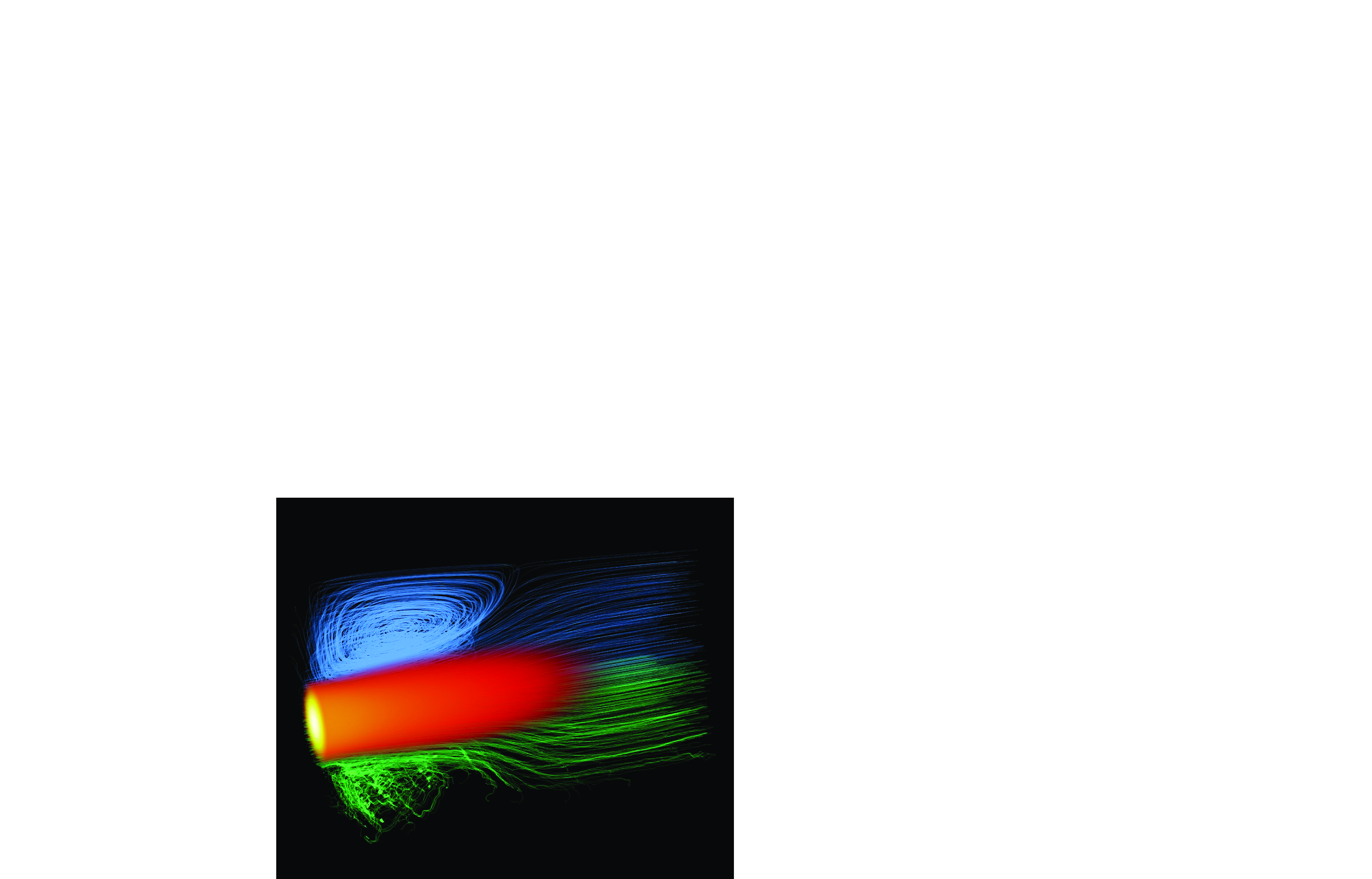
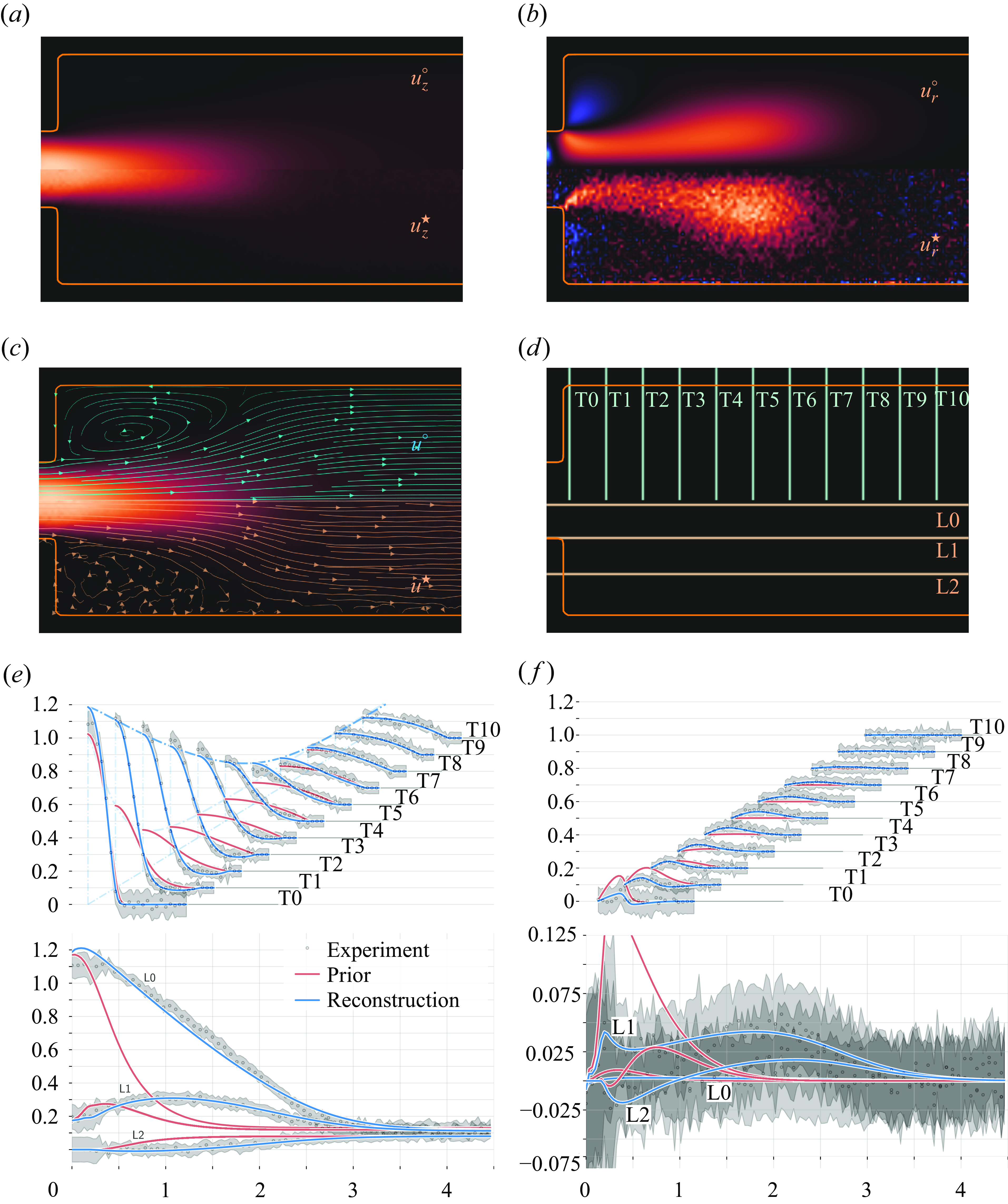
Images, streamlines and slices of reconstructed (MAP) flow, $\boldsymbol{u}^\circ$
, versus velocimetry data,
$\boldsymbol{u}^\circ$
, versus velocimetry data, $\boldsymbol{u}^\star$
. Panels (a) and (e) show the axial velocity,
$\boldsymbol{u}^\star$
. Panels (a) and (e) show the axial velocity, $u_z$
, and panels (b) and (f) show the radial velocity component,
$u_z$
, and panels (b) and (f) show the radial velocity component, $u_r$
. In panels (e) and (f), velocity is normalised by U = 20 cm s−1, and length is normalised by L = 5 mm. We separate the transverse slices in the plot by applying a vertical offset of 0.1
$u_r$
. In panels (e) and (f), velocity is normalised by U = 20 cm s−1, and length is normalised by L = 5 mm. We separate the transverse slices in the plot by applying a vertical offset of 0.1 $n$
to the
$n$
to the $n$
th slice (the horizontal offset value is immaterial).
$n$
th slice (the horizontal offset value is immaterial).
4. Joint flow field reconstruction and Carreau parameter learning
We apply algorithm1 to the non-Newtonian axisymmetric jet in order to jointly reconstruct the velocity field and learn the rheological parameters of the Carreau fluid. We use the velocimetry data (Kontogiannis et al. Reference Kontogiannis, Hodgkinson, Reynolds and Manchester2024b
), $\boldsymbol {u}^\star$
, and compute the data noise covariance,
$\boldsymbol {u}^\star$
, and compute the data noise covariance, $\mathcal {C}_{\boldsymbol {u}^\star } = \sigma ^2 \mathrm {I}$
, where
$\mathcal {C}_{\boldsymbol {u}^\star } = \sigma ^2 \mathrm {I}$
, where $\mathrm {I}$
is the identity operator, and
$\mathrm {I}$
is the identity operator, and $\sigma = 0.234$
cm s−1 (Gudbjartsson & Patz Reference Gudbjartsson and Patz1995) (for reference, peak jet velocity is
$\sigma = 0.234$
cm s−1 (Gudbjartsson & Patz Reference Gudbjartsson and Patz1995) (for reference, peak jet velocity is $\sim$
24 cm s−1.) We fix the geometry,
$\sim$
24 cm s−1.) We fix the geometry, $\Omega$
, which is known (FDA nozzle), and the outlet b.c. to
$\Omega$
, which is known (FDA nozzle), and the outlet b.c. to $\boldsymbol {g}_o \equiv \boldsymbol {0}$
, and infer the unknown Carreau parameters and the inlet b.c.,
$\boldsymbol {g}_o \equiv \boldsymbol {0}$
, and infer the unknown Carreau parameters and the inlet b.c., $\boldsymbol {g}_i$
. To test the robustness of algorithm1, we assume high uncertainty in the priors by setting the prior mean and covariance of the Carreau parameters to
$\boldsymbol {g}_i$
. To test the robustness of algorithm1, we assume high uncertainty in the priors by setting the prior mean and covariance of the Carreau parameters to $\bar {\boldsymbol {p}}_\mu = (\mu _\infty ,\delta \mu ,\lambda ,n ) = (4\times 10^{-3},10^{-1},5,1 )$
,
$\bar {\boldsymbol {p}}_\mu = (\mu _\infty ,\delta \mu ,\lambda ,n ) = (4\times 10^{-3},10^{-1},5,1 )$
, $\mathcal {C}_{\bar {\boldsymbol {p}}_\mu } = \mathrm {diag} (0.5\times 10^{-3},0.5\times 10^{-1},1,0.5 )^2$
, in SI units, and
$\mathcal {C}_{\bar {\boldsymbol {p}}_\mu } = \mathrm {diag} (0.5\times 10^{-3},0.5\times 10^{-1},1,0.5 )^2$
, in SI units, and $\rho = 1099.3$
kg m−3. Note that the prior mean corresponds to a Newtonian fluid with viscosity
$\rho = 1099.3$
kg m−3. Note that the prior mean corresponds to a Newtonian fluid with viscosity $\mu _e(\bar {\boldsymbol {p}}_{\mu }) \equiv \bar {\mu }_\infty +\bar {\delta \mu } \simeq 0.1$
Pa
$\mu _e(\bar {\boldsymbol {p}}_{\mu }) \equiv \bar {\mu }_\infty +\bar {\delta \mu } \simeq 0.1$
Pa $\cdot$
s. We set the prior mean of the inlet b.c. to
$\cdot$
s. We set the prior mean of the inlet b.c. to $\bar {\boldsymbol {g}}_i = (\mathcal {S}^*\boldsymbol {u}^\star )|_{\Gamma _i}$
, i.e. the restriction of the
$\bar {\boldsymbol {g}}_i = (\mathcal {S}^*\boldsymbol {u}^\star )|_{\Gamma _i}$
, i.e. the restriction of the $\mathcal {S}^*$
-projected data on
$\mathcal {S}^*$
-projected data on $\Gamma _i$
, and the prior covariance to
$\Gamma _i$
, and the prior covariance to $\mathcal {C}_{\bar {\boldsymbol {g}}_i} = \sigma _{\bar {\boldsymbol {g}}_i}^2\mathrm {I}$
, where
$\mathcal {C}_{\bar {\boldsymbol {g}}_i} = \sigma _{\bar {\boldsymbol {g}}_i}^2\mathrm {I}$
, where $\sigma _{\bar {\boldsymbol {g}}_i} = 1$
cm s−1. We infer the inlet b.c., instead of fixing its value to
$\sigma _{\bar {\boldsymbol {g}}_i} = 1$
cm s−1. We infer the inlet b.c., instead of fixing its value to $(\mathcal {S}^*\boldsymbol {u}^\star )|_{\Gamma _i}$
, in order to compensate for measurement noise and local imaging artefacts/biases on (or near)
$(\mathcal {S}^*\boldsymbol {u}^\star )|_{\Gamma _i}$
, in order to compensate for measurement noise and local imaging artefacts/biases on (or near) $\Gamma _i$
.
$\Gamma _i$
.
4.1. Flow field reconstruction
The reconstructed flow field, $\boldsymbol {u}^\circ$
, which is generated using algorithm1, is shown in figure 2 versus the velocimetry data,
$\boldsymbol {u}^\circ$
, which is generated using algorithm1, is shown in figure 2 versus the velocimetry data, $\boldsymbol {u}^\star$
. We define the average data-model distance by
$\boldsymbol {u}^\star$
. We define the average data-model distance by $\mathcal {E}(u_\square ) := \lvert \Omega \rvert ^{-1}\lVert u^\star _\square -\mathcal {S}u_\square \rVert _{L^2(\Omega )}$
, where
$\mathcal {E}(u_\square ) := \lvert \Omega \rvert ^{-1}\lVert u^\star _\square -\mathcal {S}u_\square \rVert _{L^2(\Omega )}$
, where $\lvert \Omega \rvert$
is the volume of
$\lvert \Omega \rvert$
is the volume of $\Omega$
, and
$\Omega$
, and $\square$
is a symbol placeholder. For the reconstructed velocity field,
$\square$
is a symbol placeholder. For the reconstructed velocity field, $\boldsymbol {u}^\circ$
, we then find
$\boldsymbol {u}^\circ$
, we then find $\mathcal {E}(u^\circ _x) = \mathcal {E}(u^\circ _y)= 0.71\sigma$
,
$\mathcal {E}(u^\circ _x) = \mathcal {E}(u^\circ _y)= 0.71\sigma$
, $\mathcal {E}(u^\circ _z) = 1.40\sigma$
, and compare this to the distance between the initial guess,
$\mathcal {E}(u^\circ _z) = 1.40\sigma$
, and compare this to the distance between the initial guess, $\boldsymbol {u}^{(0)}$
, and the data
$\boldsymbol {u}^{(0)}$
, and the data $\mathcal {E}(u^{(0)}_x) = \mathcal {E}(u^{(0)}_y) = 1.39\sigma$
,
$\mathcal {E}(u^{(0)}_x) = \mathcal {E}(u^{(0)}_y) = 1.39\sigma$
, $\mathcal {E}(u^{(0)}_z) = 5.87\sigma$
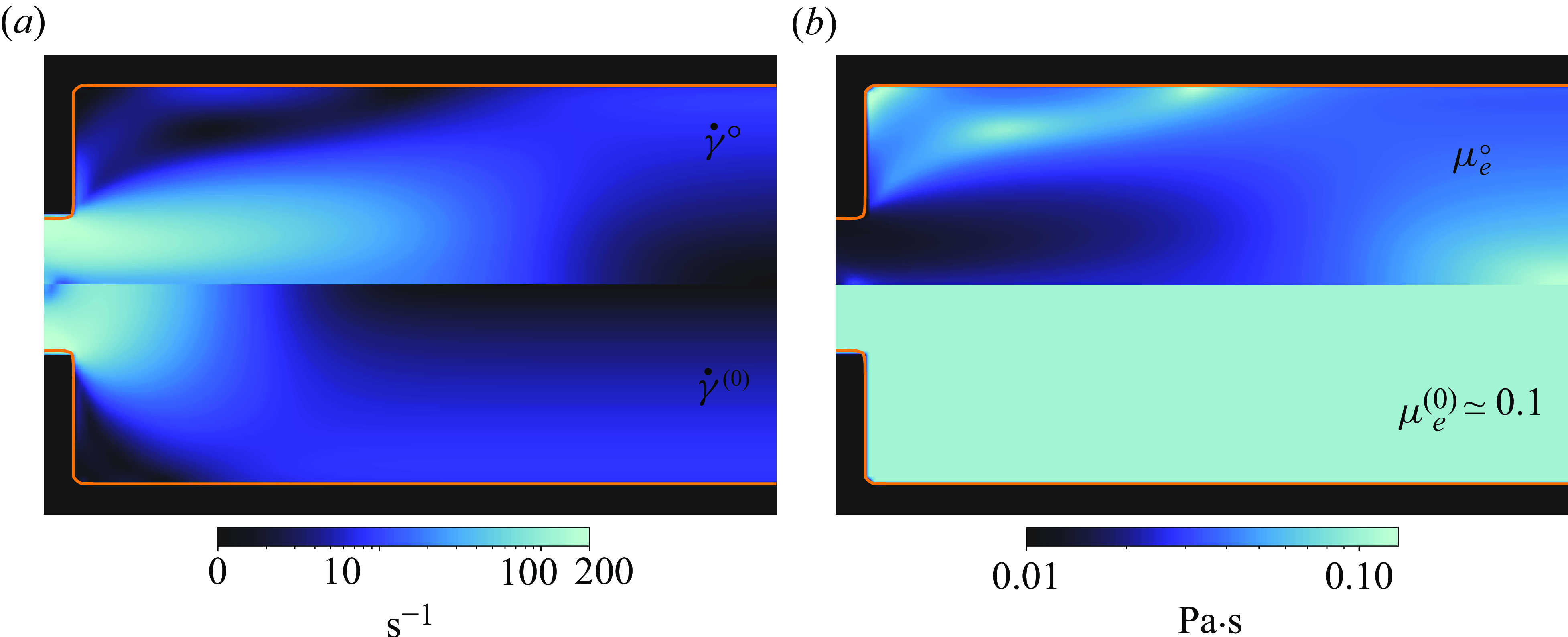
. The inferred (MAP) versus prior strain-rate magnitude,
$\mathcal {E}(u^{(0)}_z) = 5.87\sigma$
. The inferred (MAP) versus prior strain-rate magnitude, $\dot {\gamma }$
, and effective viscosity field,
$\dot {\gamma }$
, and effective viscosity field, $\mu _e(\dot {\gamma })$
, are shown in figure 3. Note that we initialise algorithm1 using the prior means, and thus
$\mu _e(\dot {\gamma })$
, are shown in figure 3. Note that we initialise algorithm1 using the prior means, and thus $\mu _e^{(0)} = \mu _e (\dot {\gamma }(\boldsymbol {u}_0);\bar {\boldsymbol {p}}_{\mu } ) \simeq 0.1$
Pa
$\mu _e^{(0)} = \mu _e (\dot {\gamma }(\boldsymbol {u}_0);\bar {\boldsymbol {p}}_{\mu } ) \simeq 0.1$
Pa $\cdot$
s. Using the reconstructed flow field,
$\cdot$
s. Using the reconstructed flow field, $\boldsymbol {u}^\circ$
, and the inferred effective viscosity field,
$\boldsymbol {u}^\circ$
, and the inferred effective viscosity field, $\mu _e^\circ$
, we find that the generalised Reynolds number of this flow is
$\mu _e^\circ$
, we find that the generalised Reynolds number of this flow is ${\textit {Re}}_g = 37.5$
, where
${\textit {Re}}_g = 37.5$
, where ${\textit {Re}}_g := \rho U_cL_c/\mu _c$
,
${\textit {Re}}_g := \rho U_cL_c/\mu _c$
, $U_c:= Q/A = 11.1$
cm s–1,
$U_c:= Q/A = 11.1$
cm s–1, $Q$
is the volumetric flow rate,
$Q$
is the volumetric flow rate, $A$
is the cross-section area before the expansion,
$A$
is the cross-section area before the expansion, $L_c = 4$
mm, and
$L_c = 4$
mm, and $\mu _c=13$
mPa is the value of the effective viscosity on the wall, before the expansion.
$\mu _c=13$
mPa is the value of the effective viscosity on the wall, before the expansion.
Inferred (MAP) versus prior strain-rate magnitude (a), $\dot{\gamma} (\textrm{s}^{-1})$
, and effective viscosity (b),
$\dot{\gamma} (\textrm{s}^{-1})$
, and effective viscosity (b), $\mu_e ({\textrm{Pa}{\cdot}\textrm{s}})$
.
$\mu_e ({\textrm{Pa}{\cdot}\textrm{s}})$
.
4.2. Carreau parameter learning
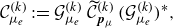
According to the optimisation log (figure 4
a), the algorithm learns the unknown N–S parameters (i.e. the Carreau parameters and the inlet b.c.) in $\sim$
20 iterations, but most of the work is done in
$\sim$
20 iterations, but most of the work is done in $\sim$
10 iterations. Using the Carreau parameters learned at every step,
$\sim$
10 iterations. Using the Carreau parameters learned at every step, $k$
, of the optimisation process, we plot the evolution of the posterior p.d.f. of
$k$
, of the optimisation process, we plot the evolution of the posterior p.d.f. of $\mu _e$
(mean,
$\mu _e$
(mean, $\mu _e^{(k)}$
, and covariance,
$\mu _e^{(k)}$
, and covariance, $\mathcal {C}^{(k)}_{\mu _e}$
) in figure 4(b). The posterior covariance of
$\mathcal {C}^{(k)}_{\mu _e}$
) in figure 4(b). The posterior covariance of $\mu _e^{(k)}$
is given by
$\mu _e^{(k)}$
is given by
 \begin{align} \mathcal {C}^{(k)}_{\mu _e} := \mathcal {G}^{(k)}_{\mu _e}\,\widetilde {\mathcal {C}}^{(k)}_{\boldsymbol {p}_{\mu }}\,\big (\mathcal {G}^{(k)}_{\mu _e}\big )^*, \end{align}
where $\mathcal {G}^{(k)}_{\mu _e}$
is the Jacobian of the Carreau fluid model (2.10) with respect to its parameters,
$\mathcal {G}^{(k)}_{\mu _e}$
is the Jacobian of the Carreau fluid model (2.10) with respect to its parameters, $\boldsymbol {p}_{\mu }$
, and
$\boldsymbol {p}_{\mu }$
, and $\widetilde {\mathcal {C}}^{(k)}_{\boldsymbol {p}_{\mu }}$
is the BFGS approximation of the posterior covariance of the Carreau parameters,
$\widetilde {\mathcal {C}}^{(k)}_{\boldsymbol {p}_{\mu }}$
is the BFGS approximation of the posterior covariance of the Carreau parameters, ${\mathcal {C}}^{(k)}_{\boldsymbol {p}_{\mu }}$
. The prior uncertainty, shown in figure 4(b) as a
${\mathcal {C}}^{(k)}_{\boldsymbol {p}_{\mu }}$
. The prior uncertainty, shown in figure 4(b) as a $\pm 3\sigma$
red shaded region, is sufficiently high and extends beyond the
$\pm 3\sigma$
red shaded region, is sufficiently high and extends beyond the $\mu _e -\dot {\gamma }$
plotting range. (To ensure that the inversion is stable with respect to prior perturbations, we performed inversions with different priors and found that the inferred posterior parameter distributions were practically the same. A sensitivity analysis with respect to the priors is, however, beyond the scope of the present study.) We observe that the posterior uncertainty of
$\mu _e -\dot {\gamma }$
plotting range. (To ensure that the inversion is stable with respect to prior perturbations, we performed inversions with different priors and found that the inferred posterior parameter distributions were practically the same. A sensitivity analysis with respect to the priors is, however, beyond the scope of the present study.) We observe that the posterior uncertainty of $\mu _e$
reduces significantly after assimilating the data in the model, and that the highest uncertainty reduction is for
$\mu _e$
reduces significantly after assimilating the data in the model, and that the highest uncertainty reduction is for $10 \lessapprox \dot {\gamma } \lessapprox 200$
s−1, which is the
$10 \lessapprox \dot {\gamma } \lessapprox 200$
s−1, which is the $\dot {\gamma }$
-range of the laminar jet (see figure 3
a). It is worth mentioning that, even though we observe a flow for which
$\dot {\gamma }$
-range of the laminar jet (see figure 3
a). It is worth mentioning that, even though we observe a flow for which $\dot {\gamma }\in [0,200]$
s−1, the region that provided the most information is that around the jet because (i) inertial effects balance viscous effects, and (ii) the local velocity-to-noise ratio is high, hence the uncertainty collapse in the jet-operating
$\dot {\gamma }\in [0,200]$
s−1, the region that provided the most information is that around the jet because (i) inertial effects balance viscous effects, and (ii) the local velocity-to-noise ratio is high, hence the uncertainty collapse in the jet-operating $\dot {\gamma }$
-range.
$\dot {\gamma }$
-range.
Optimisation log (a), and posterior p.d.f. evolution of the effective viscosity (b) and the Carreau parameters (c). In panel (c), the axes are such that $d_\sigma x := (x-\bar {x})/\sigma _{\bar {x}}$
, where
$d_\sigma x := (x-\bar {x})/\sigma _{\bar {x}}$
, where $\bar {x}$
is the prior mean and
$\bar {x}$
is the prior mean and $\sigma _{\bar {x}}$
is the prior standard deviation.
$\sigma _{\bar {x}}$
is the prior standard deviation.
The posterior p.d.f. evolution of the Carreau parameters is shown in figure 4(c). In this case, the prior uncertainty isocontours can be visualised using hyperellipsoids in $\mathbb {R}^4$
whose centres are
$\mathbb {R}^4$
whose centres are $\bar {\boldsymbol {p}}_{\mu }$
, and axis lengths are proportional to (the columns of)
$\bar {\boldsymbol {p}}_{\mu }$
, and axis lengths are proportional to (the columns of) $\mathcal {C}_{\bar {\boldsymbol {p}_\mu }}$
. To highlight the parameter uncertainty reduction after assimilating the data, we set the origin to
$\mathcal {C}_{\bar {\boldsymbol {p}_\mu }}$
. To highlight the parameter uncertainty reduction after assimilating the data, we set the origin to $\bar {\boldsymbol {p}}_{\mu }$
, and scale each dimension of
$\bar {\boldsymbol {p}}_{\mu }$
, and scale each dimension of $\mathbb {R}^4$
using (the columns of)
$\mathbb {R}^4$
using (the columns of) $\mathcal {C}_{\bar {\boldsymbol {p}}_\mu }$
. In this transformed space, the prior uncertainty isocontours are hyperspheres, and the posterior uncertainty isocontours are hyperellipsoids, whose slices are shown in figure 4(c). It is interesting to note that, after assimilating the velocimetry data, the posterior uncertainty collapses along the axes
$\mathcal {C}_{\bar {\boldsymbol {p}}_\mu }$
. In this transformed space, the prior uncertainty isocontours are hyperspheres, and the posterior uncertainty isocontours are hyperellipsoids, whose slices are shown in figure 4(c). It is interesting to note that, after assimilating the velocimetry data, the posterior uncertainty collapses along the axes $n$
,
$n$
, $\delta \mu$
, whilst it slightly decreases along the axes
$\delta \mu$
, whilst it slightly decreases along the axes $\mu _\infty$
,
$\mu _\infty$
, $\lambda$
. This indicates that there is insufficient information in the data to further collapse the prior uncertainties of
$\lambda$
. This indicates that there is insufficient information in the data to further collapse the prior uncertainties of $\lambda$
and
$\lambda$
and $\mu _\infty$
.
$\mu _\infty$
.
It is known that for models with univariate design (e.g. shear rate, $\dot {\gamma }$
) and observable variables (e.g. effective viscosity,
$\dot {\gamma }$
) and observable variables (e.g. effective viscosity, $\mu _e$
) in order to learn the most about the unknown parameters (e.g.
$\mu _e$
) in order to learn the most about the unknown parameters (e.g. $\boldsymbol {p}_{\mu }$
) we need to perform experiments with the design parameters at which the model is most uncertain (Yoko & Juniper Reference Yoko and Juniper2024b
, § 4.1). Here, figure 4(b) shows that the model is most uncertain for
$\boldsymbol {p}_{\mu }$
) we need to perform experiments with the design parameters at which the model is most uncertain (Yoko & Juniper Reference Yoko and Juniper2024b
, § 4.1). Here, figure 4(b) shows that the model is most uncertain for $\dot {\gamma } \ll 10$
s−1 and
$\dot {\gamma } \ll 10$
s−1 and $\dot {\gamma } \gg 200$
s−1. Consequently, in order to further collapse the uncertainty of
$\dot {\gamma } \gg 200$
s−1. Consequently, in order to further collapse the uncertainty of $\lambda$
and
$\lambda$
and $\mu _\infty$
, we require more (or higher SNR) flow-MRI data for
$\mu _\infty$
, we require more (or higher SNR) flow-MRI data for $\dot {\gamma } \ll 10$
s−1 and
$\dot {\gamma } \ll 10$
s−1 and $\dot {\gamma } \gg 200$
s−1. In particular, since we have used flow-MRI data of a jet for which
$\dot {\gamma } \gg 200$
s−1. In particular, since we have used flow-MRI data of a jet for which $\dot {\gamma }\in [0,200]$
s−1, we would require new experiments with (i) higher SNR, since information at low velocity magnitudes, i.e.
$\dot {\gamma }\in [0,200]$
s−1, we would require new experiments with (i) higher SNR, since information at low velocity magnitudes, i.e. $\dot {\gamma } \ll 10$
s−1, is corrupted by noise, and (ii) higher velocity magnitudes (for the same geometry), since information at
$\dot {\gamma } \ll 10$
s−1, is corrupted by noise, and (ii) higher velocity magnitudes (for the same geometry), since information at $\dot {\gamma } \gg 200$
s−1 is missing from the current experiment.
$\dot {\gamma } \gg 200$
s−1 is missing from the current experiment.
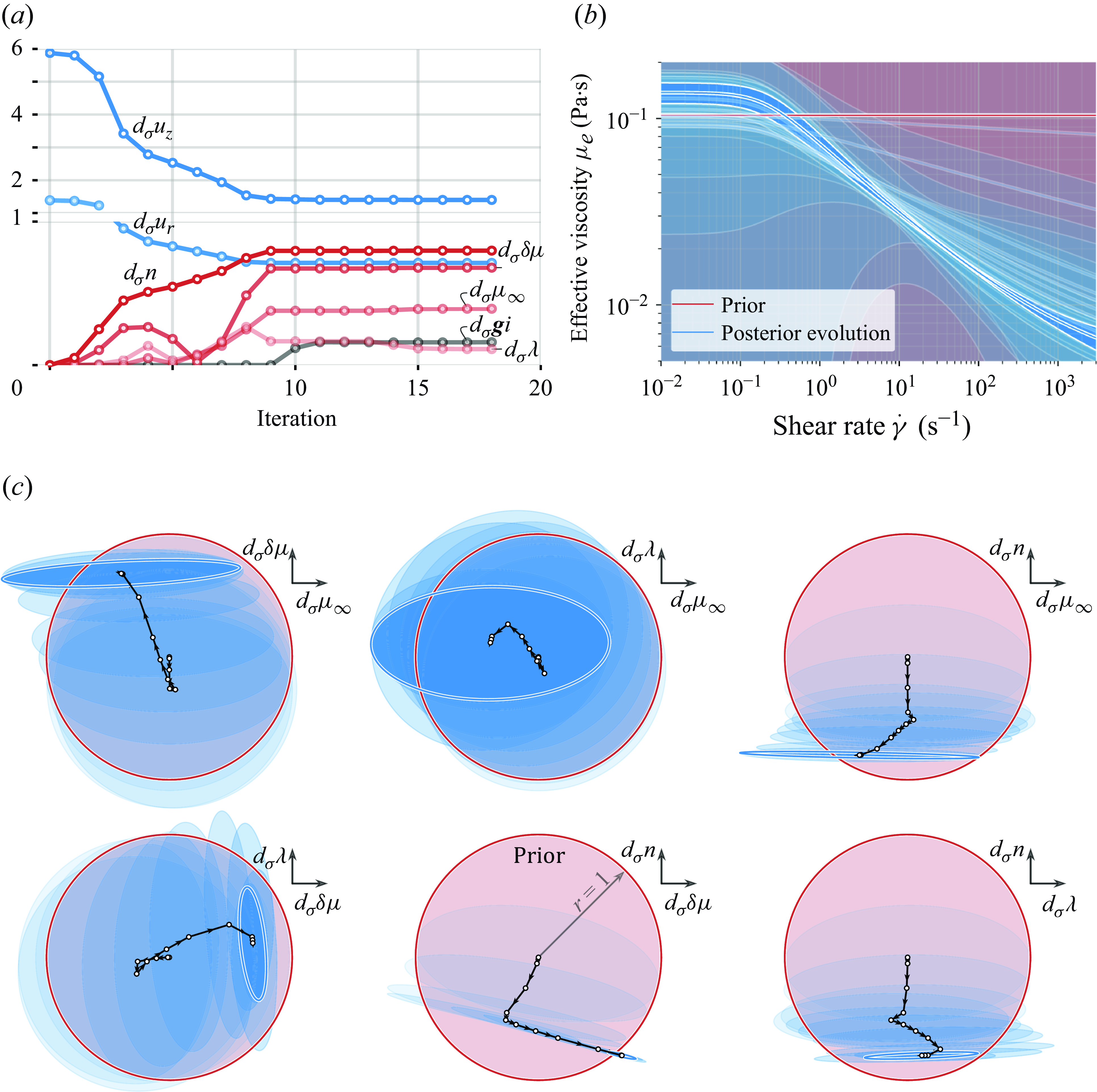
4.3. Validation via an independent rheometry experiment
Steady-shear rheometry of the test solution was conducted using a Netzsch Kinexus rheometer with a $\varnothing$
27.5 mm cup and a
$\varnothing$
27.5 mm cup and a $\varnothing$
25 mm bob geometry, at the same temperature as the flow-MRI experiment. The experiment was conducted to validate the Carreau parameters learned from the flow-MRI data (§ 4.2) against rheometry data. To find the most likely Carreau parameters that fit the rheometry data, we use Bayesian inversion (see § 2). In this case, operator
$\varnothing$
25 mm bob geometry, at the same temperature as the flow-MRI experiment. The experiment was conducted to validate the Carreau parameters learned from the flow-MRI data (§ 4.2) against rheometry data. To find the most likely Carreau parameters that fit the rheometry data, we use Bayesian inversion (see § 2). In this case, operator $\mathcal {Z}$
corresponds to the Carreau model, given by the explicit relation (2.10), and operator
$\mathcal {Z}$
corresponds to the Carreau model, given by the explicit relation (2.10), and operator $\mathcal {G}$
corresponds to the Jacobian of the Carreau model with respect to its parameters. We use the same prior as in § 4. Because the prior uncertainty is sufficiently high relative to the noise variance, the bias it introduces to the model fit is negligible. The Carreau parameters learned from flow-MRI versus rheometry are shown in figure 5. We observe that the parameters learned from flow-MRI agree well with rheometry data, considering uncertainties (figure 5
b), and that the learned effective viscosity field fits the rheometry data (figure 5
a). As in the case of learning from flow-MRI, it is not possible to infer
$\mathcal {G}$
corresponds to the Jacobian of the Carreau model with respect to its parameters. We use the same prior as in § 4. Because the prior uncertainty is sufficiently high relative to the noise variance, the bias it introduces to the model fit is negligible. The Carreau parameters learned from flow-MRI versus rheometry are shown in figure 5. We observe that the parameters learned from flow-MRI agree well with rheometry data, considering uncertainties (figure 5
b), and that the learned effective viscosity field fits the rheometry data (figure 5
a). As in the case of learning from flow-MRI, it is not possible to infer $\lambda$
and
$\lambda$
and $\mu _\infty$
with high certainty when data,
$\mu _\infty$
with high certainty when data, $\mu _e(\dot {\gamma })$
, for
$\mu _e(\dot {\gamma })$
, for $\dot {\gamma } \ll 10$
s−1 and
$\dot {\gamma } \ll 10$
s−1 and $\dot {\gamma } \gg 200$
s−1 are missing (or the measurement uncertainty is high).
$\dot {\gamma } \gg 200$
s−1 are missing (or the measurement uncertainty is high).
Learned Carreau fit to rheometry data, learned model parameters (MAP estimates), and assumed priors. Uncertainties in the figures correspond to $3\sigma$
intervals.
$3\sigma$
intervals.
5. Summary and conclusions
We have formulated a Bayesian inverse N–S problem that assimilates velocimetry data of 3-D steady incompressible flow in order to jointly reconstruct the flow field and learn the unknown N–S parameters. By incorporating a Carreau shear-thinning viscosity model into the N–S problem, we devise an algorithm that learns the Carreau parameters of a shear-thinning fluid, and estimates their uncertainties, from velocimetry data alone. Then we conduct a flow-MRI experiment to obtain velocimetry data of an axisymmetric laminar jet through an idealised medical device (FDA nozzle), for a blood analogue fluid. We show that the algorithm successfully reconstructs the noisy flow field, and, at the same time, learns the Carreau parameters and their uncertainties. To ensure that the learned Carreau parameters explain the rheology of the fluid, instead of simply fitting the velocimetry data, we conduct an additional rheometry experiment. We find that the Carreau parameters learned from the flow-MRI data alone are in very good agreement with the parameters learned from the rheometry experiment (taking into account their uncertainties), and that the learned effective viscosity field fits the rheometry data. In this paper we have applied the algorithm to a Carreau fluid. The present algorithm, however, accepts any generalised Newtonian fluid, as long as the model is (weakly) differentiable. More complicated non-Newtonian behaviour, such as viscoelasticity, can be learned from velocimetry data if a viscoelastic model (e.g. Oldroyd-B fluid) is incorporated into the N–S problem. The present study has demonstrated the method on a single dataset. In future work we will extend this to more test cases and different experimental configurations.
Acknowledgements.
Thanks to M. Yoko (Cambridge) for useful discussions on optimal experiment design, and for providing the script that straightens and centres axisymmetric object images.
Funding.
The authors are supported by EPSRC National Fellowships in Fluid Dynamics (NFFDy), grants EP/X028232/1 (AK), EP/X028089/1 (RH) and EP/X028321/1 (ELM).
Declaration of interests.
The authors report no conflict of interest.
Data availability statement.
The experimental flow-MRI data used in this study are available at https://doi.org/10.17863/CAM.113320.


 Open access