




1 Introduction
Driven by growing requirements for high-power operation, developing laser sources that sustain efficient, stable output under power scaling has become a central challenge for both academic and industrial communities[ Reference Lebegue, De Sousa, Rapenau, Badarau, Andrieu, Audebert, Druon and Papadopoulos 1 – Reference Lubin, Hughes, Bible, Bublitz, Arriola, Motta, Suen, Johansson, Riley, Sarvian, Clayton-Warwick, Wu, Milich, Oleson, Pryor, Krogen, Kangas and O’Neill 4 ]. Despite rapid progress in high-power laser technology, conventional solid-state lasers remain severely constrained by thermal effects during power scaling. As the pump power increases, part of the population inversion in the gain medium undergoes nonradiative relaxation, releasing energy as heat rather than photons, which leads to thermal-lens effects, stress-induced birefringence, beam distortion and spectral broadening[ Reference Weber, Neuenschwander and Weber 5 – Reference Söderlund, Ponsoda, Koplow and Honkanen 7 ]. These thermally induced effects lead to cavity-mode mismatch and beam-quality degradation, ultimately limiting further improvement in output power and beam quality.
One promising route toward overcoming this bottleneck is the use of Raman lasers based on stimulated Raman scattering, which have emerged as a major direction for high-power laser development. These lasers utilize the third-order nonlinear polarization response of materials for optical-frequency conversion, in which energy transfer is driven by photon–phonon interactions rather than population inversion, thus avoiding the substantial heat deposition associated with upper-level lifetimes and quantum defects in traditional gain media. Moreover, Raman conversion typically exhibits a small quantum defect and a limited frequency shift between the pump and Stokes waves, substantially reducing the heat load per unit output power and enabling higher brightness and higher-power operation under strong pumping[ Reference Sarang and Richardson 8 – Reference Bai, Williams, Jasbeer, Sarang, Kitzler, McKay and Mildren 11 ]. Among various Raman media, single-crystal diamond is regarded as an ideal material for constructing high-power Raman lasers owing to its outstanding properties. Diamond exhibits ultrahigh thermal conductivity and an extremely low thermal-expansion coefficient, enabling efficient heat dissipation and suppression of thermal distortion under high pump powers[ Reference An, Zhao, Yang, Zhai, Dai, Wang, Li, Hu, Sun, Fan, Wu and Niu 12 – Reference Lubeigt, Bonner, Hastie, Dawson, Burns and Kemp 14 ]; it also provides a high Raman gain coefficient, a broad optical-transmission window and a high damage threshold, supporting wavelength conversion from the ultraviolet to the mid-infrared and enabling Raman self-cleaning to improve beam quality[ Reference Bai, Zhang, Zhang, Tan, Chen, Fan, Ding, Qi, Yan, Wang, Wang and Lu 15 – Reference Jasbeer, Williams, Kitzler, McKay and Mildren 21 ]. Benefiting from these exceptional properties, diamond Raman laser (DRL) technology has made significant progress in recent years, with continuous-wave output powers reaching several hundred watts and quasi-continuous-wave powers exceeding the kilowatt level, demonstrating great potential for high-power and high-beam-quality laser applications[ Reference Li, Sun, Jiang, Yang and Feng 22 – Reference Chen, Cui, Li, Zhang, Cai, Ding, Qi, Yan, Wang and Lu 24 ].
However, experimental studies show that despite the extremely high thermal conductivity of diamond, its thermo-optic effects remain non-negligible. In 2015, Williams et al. [ Reference Williams, Nold, Strecker, Kitzler, McKay, Schreiber and Mildren 25 ] investigated an external-cavity DRL using dual-pass pulsed and continuous-wave pumping. A Stokes output power of 138 W was achieved at a pump power of 309 W, and pronounced noise associated with thermal effects was observed. In 2016, Pashinin et al. [ Reference Pashinin, Ralchenko, Bolshakov, Ashkinazi, Gorbashova, Yurov and Konov 26 ] found that the first-order Stokes conversion efficiency decreased when the pump energy exceeded 4 mJ, attributing this behavior to transient thermal accumulation within the crystal. In 2019, Antipov et al. [ Reference Antipov, Sabella, Williams, Kitzler, Spence and Mildren 23 ] reported an improvement in output beam quality in an external-cavity diamond Raman laser as the first-Stokes output peak power increased above approximately 0.4 kW, with the beam-quality factor M 2 decreasing at higher power levels. This behavior was interpreted as evidence of thermal-lens development in the diamond. The thermally induced change in the cavity mode was considered to improve the spatial overlap between the fundamental Stokes mode and the pump field, thereby favoring fundamental-mode operation and suppressing higher-order transverse-mode contributions. In 2020, Antipov et al. further analyzed this thermal-lensing behavior through combined beam-quality measurements, divergence measurements and theoretical modeling[ Reference Antipov, Williams, Sabella, Kitzler, Berhane, Spence and Mildren 27 ]. More recently, Zhang et al. [ Reference Zhang, Li, Chen, Chen, Zheng, Wang, Ding, Wang, Lu and Bai 28 ] investigated the thermodynamics and performance-degradation mechanisms of continuous-wave DRLs, showing that thermal-lens effects alter the intracavity field distribution, degrade pump–Stokes mode matching and lead to gain reduction, power saturation and even roll-off. These findings collectively indicate that passive reliance on high-thermal-conductivity materials alone is insufficient, and achieving stable high-power laser operation requires new active compensation strategies and theoretical guidance.
To mitigate the thermal limitations in DRLs, researchers have explored various thermal management and compensation approaches. On the one hand, passive strategies such as using high-thermal-conductivity substrates and optimizing crystal mounting and heat sink structures can reduce the average temperature rise, but they offer limited improvement in internal temperature uniformity and thus limited suppression of thermal effects[ Reference Zhang, Li, Chen, Chen, Zheng, Wang, Ding, Wang, Lu and Bai 28 ]. On the other hand, some studies adjust the cavity length or mirror curvature to optimize cavity design and compensate for mode-field mismatch, but these methods are largely empirical and lack systematic modeling or quantitative criteria[ Reference Bai, Zhang, Wang, Gao, Zhang, Yang, Wang, Lu and Mildren 29 ]. Moreover, existing thermo-optical coupling simulations are mostly based on steady-state models that describe only thermal field distributions at fixed power, making it difficult to capture cavity-mode evolution under varying power levels[ Reference Gong, Zhang, Lin, Yang, Fu, Ma, Hu, Dong and Shan 30 , Reference Ding, Li, Chen, Cai, Bai, Qi, Yan, Wang and Lu 31 ]. Thus, developing a self-consistent modeling framework describing the coupling among pump power, thermal-lens effects and cavity modes, together with steady-state compensation, remains a key research challenge.
Motivated by these challenges, we construct a chained modeling framework that describes the coupled relationships among pump power, thermal load, thermal-lens effects and cavity-mode matching. Within this framework, the relationship between pump power and cavity-length compensation is quantified, and a peak–valley co-location (PVC) criterion based on self-feedback from output power is introduced to determine the optimal compensation point. Experimental results show that this method significantly improves the output power and stability of DRLs, enabling steady-state optimization under high-power operation. This study unifies power amplification, thermal management and cavity-mode control within a single framework, providing new theoretical and engineering foundations for active steady-state control of high-power solid-state lasers, deepening the understanding of multiphysics coupling mechanisms, and laying the groundwork for future research on thermal compensation and mode-field optimization.
2 Experimental setup and results
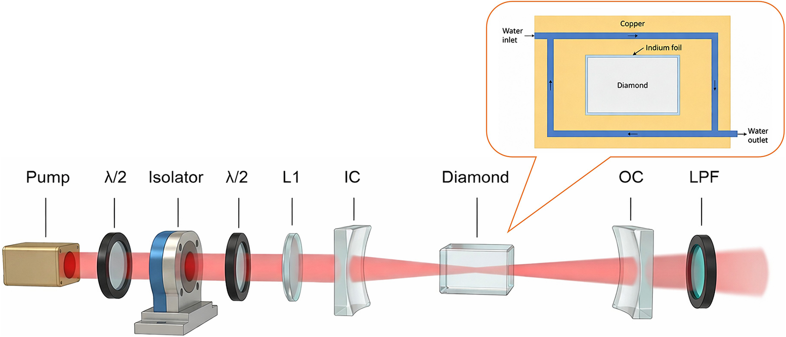
Figure 1 illustrates the configuration of the external-cavity DRL system used in the experiment. The pump source is a continuous-wave fiber laser operating at 1064 nm with a maximum output power of 500 W. After passing through an optical isolator, the pump beam enters the system, ensuring unidirectional propagation with continuously adjustable output power. Prior to entering the Raman cavity, a second half-wave plate is used to align the pump polarization with the <111> axis of the diamond crystal to maximize the Raman gain. The pump beam is then focused at the crystal center using a 75 mm focal-length lens (L1), producing a beam waist radius of approximately 28 μm. The diamond crystal, with a cross-sectional area of 4 mm × 2 mm and a length of 8 mm along the optical axis, is positioned at the focal point of the resonator. In addition, both facets are coated with anti-reflection coatings for the 1064 nm pump, 1240 nm first-order Stokes and 1485 nm second-order Stokes wavelengths. The diamond crystal is wrapped in indium foil and mounted on a water-cooled copper holder connected to a recirculating chiller with a cooling capacity of 3000 W, a set temperature of 20°C and a flow rate of 10 L min−1. The resonator adopts a near-concentric configuration with a total length of approximately 103 mm, resulting in an intrinsic waist radius of 44 μm for the first-order Stokes mode. The concave input coupler (IC) has a curvature radius of 50 mm, providing high transmission at 1064 and 1485 nm while being highly reflective at 1240 nm. The output coupler (OC), also with a 50 mm curvature radius, is highly reflective at 1064 nm, highly transmissive at 1485 nm and provides approximately 0.7% transmission at 1240 nm. A long-pass filter (LPF) is used to remove residual pump light and obtain a clean Stokes output.
Schematic diagram of the external-cavity diamond Raman laser structure. Inset: schematic illustration showing the cooling arrangement of the diamond crystal.

Figure 1 Long description
From left to right, the main diagram shows a sequence of labeled optical components: Pump, lambda forward slash 2, Isolator, lambda forward slash 2, L 1, I C, Diamond, O C, and L P F. A red laser beam passes through each component in order. The diamond crystal is centrally positioned in the optical path. An inset at the upper right details the cooling arrangement: the outermost layer is labeled Copper, with a blue path indicating water inlet and outlet channels running along the perimeter. Inside the copper, a rectangular Indium foil layer surrounds the central Diamond crystal. Arrows in the inset show water flow direction around the diamond.
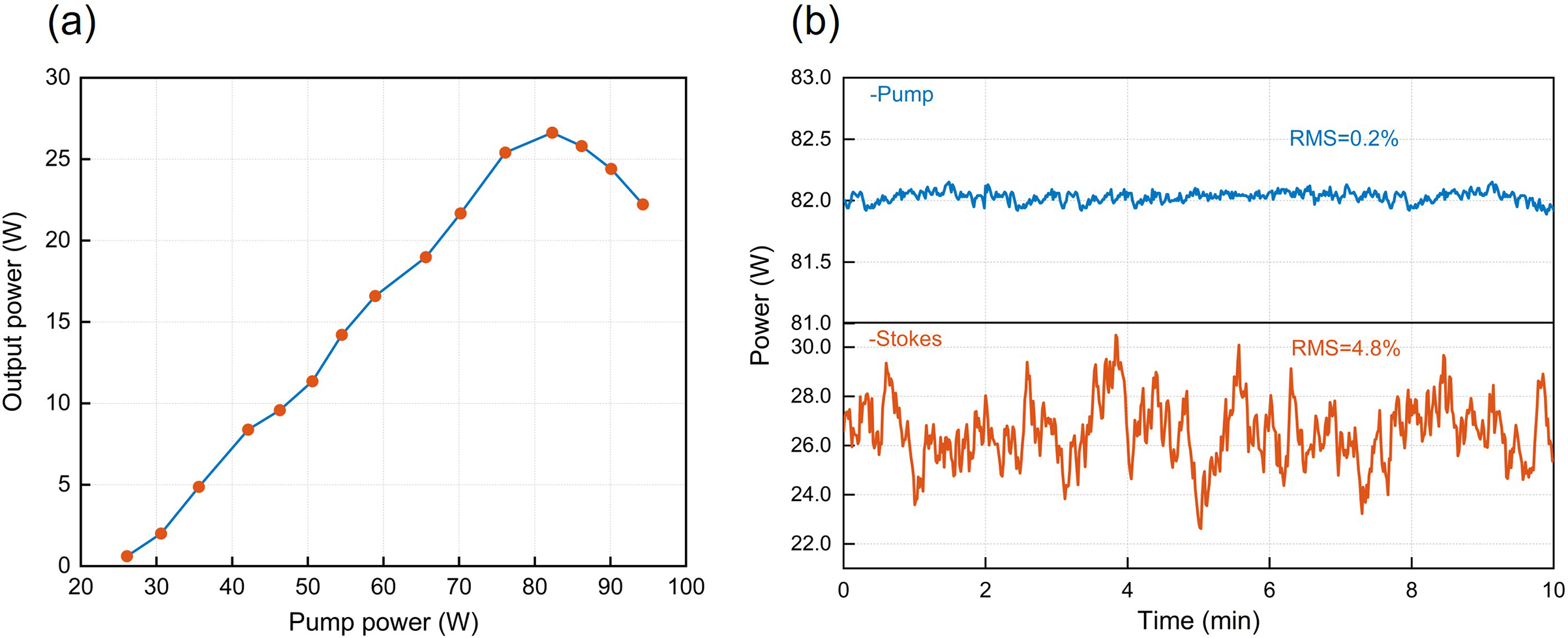
With the cavity length fixed, Figure 2 shows the first-order Stokes output power and the corresponding power characteristics of the external-cavity DRL. As shown in Figure 2(a), the threshold for first-order Stokes generation is approximately 26 W. Once the pump power exceeds the threshold, the output power increases rapidly and grows nearly linearly in the 26–82 W pump power range. At a pump power of 82 W, the output reaches a maximum of about 27 W, corresponding to an optical-to-optical efficiency of approximately 33%. However, further increasing the pump power causes the output to decline, exhibiting a typical non-monotonic response. This behavior indicates that thermal effects begin to dominate in the high-power regime. Despite diamond’s exceptionally high thermal conductivity, the strong focusing of the pump still induces nonuniform temperature rises inside the crystal, altering the refractive-index distribution and forming an equivalent thermal lens. When the cavity length is fixed, variations in the thermal-lens focal length disrupt intracavity-mode matching, reducing the spatial overlap between the Stokes and pump beams and thus decreasing Raman gain and causing power degradation.
Output power characteristics and stability of the external-cavity diamond Raman laser. (a) First-order Stokes output power as a function of pump power. (b) Power stability of the pump and Stokes beams at maximum output power.

Figure 2 Long description
A two-panel figure labeled a and b.
Panel a is a line graph with orange circular data points. The horizontal x-axis is labeled Pump power in Watts W, ranging from 20 to 100. The vertical y-axis is labeled Output power in Watts W, ranging from 0 to 30. The data shows a linear increase in output power from approximately 1 Watt at 26 Watts pump power up to a peak of 26.6 Watts at 82 Watts pump power. Beyond this peak, the output power decreases to approximately 22 Watts at 94 Watts pump power.
Panel b is a multi-series line graph showing power stability over time. The horizontal x-axis is labeled Time in minutes min, ranging from 0 to 10. The vertical y-axis is labeled Power in Watts W. The graph is split into two sections.
* The top section shows the Pump beam in blue, fluctuating around 85.0 Watts with a label R M S equals 0.2 percent. The line shows very low amplitude noise.
* The bottom section shows the Stokes beam in orange, fluctuating between 23 and 30 Watts with a label R M S equals 4.8 percent. This line shows significantly higher amplitude oscillations compared to the pump beam.
Figure 2(b) shows the temporal stability of the pump and Stokes beams under conditions corresponding to the maximum output power. As shown, the pump power fluctuates minimally (root mean square (RMS) ≈ 0.2%) over a 10-minute measurement window, indicating that the pump source is intrinsically highly stable. In contrast, the Stokes power exhibits significantly larger fluctuations, with an RMS of approximately 4.8% and a random fluctuation pattern. This discrepancy indicates that the system instability mainly arises from intracavity thermo-optical perturbations rather than pump noise. Over time, dynamic variations in the crystal temperature field cause fluctuations in the equivalent thermal focal length, shifting the cavity mode away from optimal matching and inducing gain and loss fluctuations.
Combining the results of Figures 2(a) and 2(b), the system exhibits good linear amplification and high efficiency at low to moderate pump power, but becomes limited at high powers by thermal-lens effects and mode mismatch. The simultaneous power roll-off and temporal instability indicate that as the pump approaches the thermal-saturation threshold, the system enters a critical region in which the cavity-mode position becomes highly sensitive to variations in the thermal focal length. Therefore, dynamically compensating the mode-field drift induced by the thermal lens could restore pump–Stokes spatial overlap, thereby improving both the output power and the power stability.
3 Chained modeling and cavity-length compensation strategy
3.1 Theoretical modeling and compensation mechanism
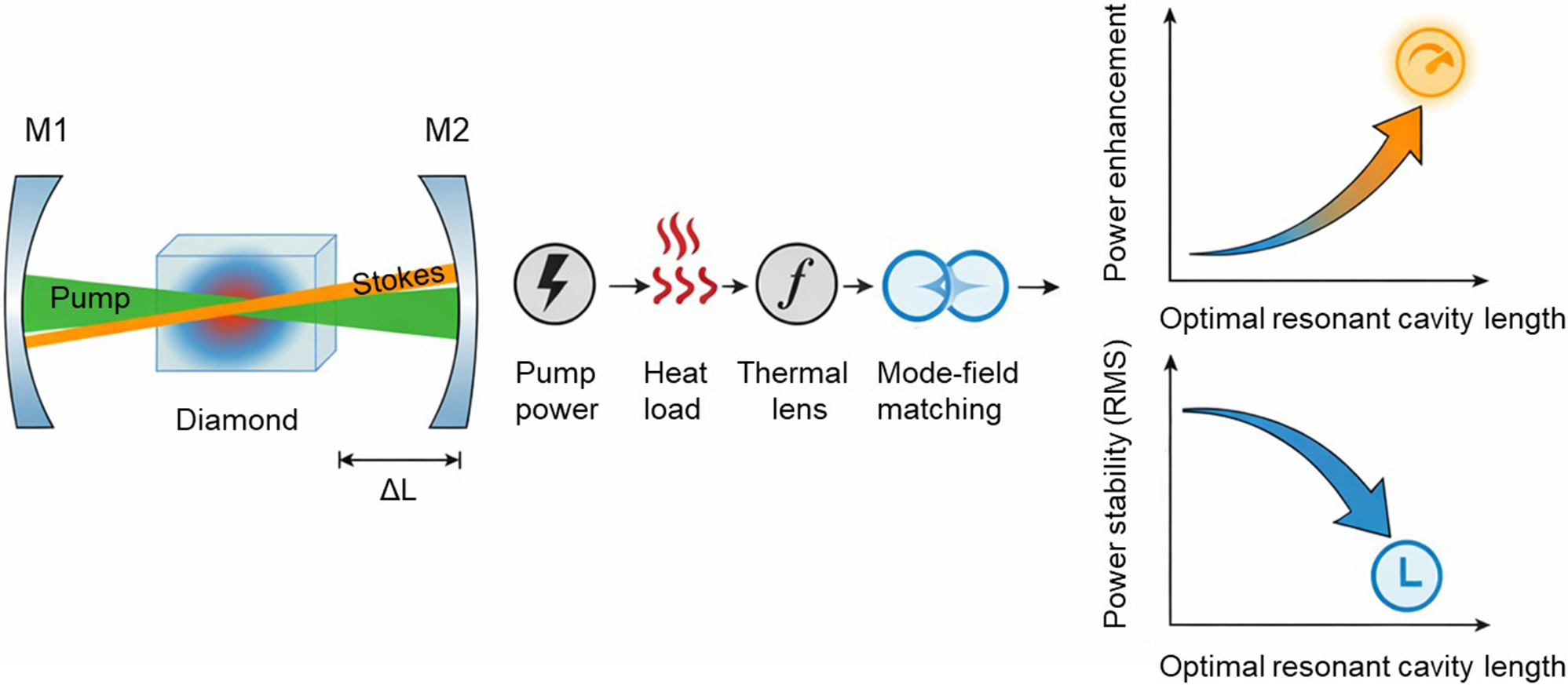
In high-power continuous-wave DRLs, residual absorption and the quantum defect of the pump and Stokes waves in the crystal are converted into heat, forming a nonuniform temperature field that induces thermo-optic and thermo-elastic effects[ Reference Bai, Zhang, Wang, Gao, Zhang, Yang, Wang, Lu and Mildren 29 – Reference Ding, Li, Chen, Cai, Bai, Qi, Yan, Wang and Lu 31 ]. The combined action of these effects makes the crystal behave as an effective thermal lens, thereby modifying the intracavity-mode parameters and degrading the output performance. To systematically describe the chained coupling from pump power to heat deposition, thermal lensing, mode-field matching and cavity-length compensation, a chained modeling framework is developed that maps the pump power Pp to the cavity-length compensation ΔL. The overall chained modeling framework and the corresponding cavity-length compensation mechanism are schematically illustrated in Figure 3. As the pump power increases, the associated heat load forms an effective thermal lens within the diamond crystal. The cavity-length compensation ΔL is then adjusted to restore pump–Stokes mode-field matching, which in turn enhances the Stokes output power and suppresses power fluctuations, as qualitatively illustrated in the right-hand panels.
Schematic illustration of the chained modeling and cavity-length compensation mechanism in a high-power continuous-wave diamond Raman laser.

Figure 3 Long description
The diagram is divided into three main sections from left to right.
1. Laser Cavity Setup: On the far left, a diamond crystal is positioned between two curved mirrors labeled M 1 and M 2. A green Pump beam and an orange Stokes beam intersect within the diamond, which shows a red and blue thermal gradient at its center. Below mirror M 2, a double-headed arrow indicates a change in length labeled Delta L.
2. Chained Modeling Flow: A horizontal sequence of four circular icons connected by arrows represents the causal mechanism.
- First is a lightning bolt icon labeled Pump power.
- Second is a red wavy heat icon labeled Heat load.
- Third is a circle containing the letter f labeled Thermal lens.
- Fourth is two overlapping blue circles labeled Mode-field matching.
3. Performance Graphs: Two line graphs are stacked on the right. Both share an x-axis labeled Optimal resonant cavity length.
- The top graph shows Power enhancement on the y-axis. An orange arrow curves upward, indicating an exponential increase toward a gauge icon.
- The bottom graph shows Power stability R M S on the y-axis. A blue arrow curves downward, indicating a decrease toward a circle containing the letter L.
Under steady-state conditions, the relationship between pump power and first-order Stokes output power in an external-cavity Raman laser is given by the following[ Reference Kitzler, McKay, Spence and Mildren 32 ]:

Here, T is the transmission of the OC at the Stokes wavelength,
$\alpha$
 is the crystal absorption coefficient, L is the crystal length,
$\eta ={\lambda}_{p}/{\lambda}_{s}$
is the crystal absorption coefficient, L is the crystal length,
$\eta ={\lambda}_{p}/{\lambda}_{s}$
 is the quantum conversion efficiency and G is the effective stimulated Raman gain coefficient. For a given pump power
${P}_p$
is the quantum conversion efficiency and G is the effective stimulated Raman gain coefficient. For a given pump power
${P}_p$
 , the corresponding Stokes output power
${P}_s$
, the corresponding Stokes output power
${P}_s$
 can be obtained by numerically inverting Equation (1). On this basis, the heat load arising from the quantum defect and pump/Stokes absorption can be expressed as follows[
Reference Feve, Shortoff, Bohn and Brasseur
33
]:
can be obtained by numerically inverting Equation (1). On this basis, the heat load arising from the quantum defect and pump/Stokes absorption can be expressed as follows[
Reference Feve, Shortoff, Bohn and Brasseur
33
]:

Here,
${\lambda}_p$
 and
${\lambda}_s$
and
${\lambda}_s$
 are the pump and Stokes wavelengths, respectively, and
${\alpha}_p$
are the pump and Stokes wavelengths, respectively, and
${\alpha}_p$
 and
${\alpha}_s$
and
${\alpha}_s$
 denote the corresponding dimensionless effective absorptances of the diamond crystal[
Reference Friel, Geoghegan, Twitchen and Scarsbrook
34
]. Under the combined action of thermo-optic and thermo-elastic effects, the crystal can be treated as an equivalent thermal lens with focal length f, which approximately follows the next equation[
Reference Williams, Nold, Strecker, Kitzler, McKay, Schreiber and Mildren
25
, Reference Antipov, Williams, Sabella, Kitzler, Berhane, Spence and Mildren
27
, Reference Li, Ding, Bai, Yang, Li, Tang, Zhang, Qi, Wang and Lu
35
, Reference Tu, Ma, Hu, Jiang, Shen, Zong, Yi, Yuan, Wang and Wang
36
]:
denote the corresponding dimensionless effective absorptances of the diamond crystal[
Reference Friel, Geoghegan, Twitchen and Scarsbrook
34
]. Under the combined action of thermo-optic and thermo-elastic effects, the crystal can be treated as an equivalent thermal lens with focal length f, which approximately follows the next equation[
Reference Williams, Nold, Strecker, Kitzler, McKay, Schreiber and Mildren
25
, Reference Antipov, Williams, Sabella, Kitzler, Berhane, Spence and Mildren
27
, Reference Li, Ding, Bai, Yang, Li, Tang, Zhang, Qi, Wang and Lu
35
, Reference Tu, Ma, Hu, Jiang, Shen, Zong, Yi, Yuan, Wang and Wang
36
]:

Here,
$K$
 is the thermal conductivity,
${w}_0$
is the thermal conductivity,
${w}_0$
 is the pump beam waist radius,
$\mathrm{d}n$
is the pump beam waist radius,
$\mathrm{d}n$
 /
$\mathrm{d}T$
/
$\mathrm{d}T$
 is the thermo-optic coefficient,
${n}_0$
is the thermo-optic coefficient,
${n}_0$
 denotes the refractive index of diamond at the Stokes wavelength,
$\nu$
denotes the refractive index of diamond at the Stokes wavelength,
$\nu$
 is the Poisson ratio,
${\alpha}_T$
is the Poisson ratio,
${\alpha}_T$
 is the thermal-expansion coefficient and
${C}_{r,\varPhi }$
is the thermal-expansion coefficient and
${C}_{r,\varPhi }$
 is the stress-optic constant. Equations (1)–(3) establish the mapping
${P}_p$
is the stress-optic constant. Equations (1)–(3) establish the mapping
${P}_p$
 →
${P}_s$
→
${P}_s$
 →
$Q$
→
$Q$
 →
$f$
→
$f$
 ; that is, for a given pump power
${P}_p$
; that is, for a given pump power
${P}_p$
 , the corresponding effective thermal focal length f can be directly obtained.
In the cavity-mode analysis, the diamond crystal is modeled as a medium of length L and refractive index n, with its center plane taken as the reference plane. The two end mirrors
$\mathrm{M}_1$
 and
$\mathrm{M}_2$
and
$\mathrm{M}_2$
 have curvature radii
${R}_1$
have curvature radii
${R}_1$
 and
${R}_2$
and
${R}_2$
 , respectively, and the geometric distance between the mirrors is
$L_c$
, respectively, and the geometric distance between the mirrors is
$L_c$
 . In the cold cavity, the left and right arm lengths are
$L_{1,0}$
. In the cold cavity, the left and right arm lengths are
$L_{1,0}$
 and
$L_{2,0}$
and
$L_{2,0}$
 satisfying
$L_c = L_{1,0} + L_{2,0}$
satisfying
$L_c = L_{1,0} + L_{2,0}$
 . By slightly adjusting the position of the right-hand mirror
$\mathrm{M}_2$
. By slightly adjusting the position of the right-hand mirror
$\mathrm{M}_2$
 , cavity-length compensation
$\Delta L$
, cavity-length compensation
$\Delta L$
 is introduced such that
$L_{2}(\Delta L) = L_{2,0} + \Delta L ~\rm{and}~ \textit{L}_\textit{c}(\Delta \textit{L}) = \textit{L}_{1,0} + \textit{L}_{2,0} + \Delta \textit{L} = \textit{L}_\textit{c} + \Delta \textit{L}$
is introduced such that
$L_{2}(\Delta L) = L_{2,0} + \Delta L ~\rm{and}~ \textit{L}_\textit{c}(\Delta \textit{L}) = \textit{L}_{1,0} + \textit{L}_{2,0} + \Delta \textit{L} = \textit{L}_\textit{c} + \Delta \textit{L}$
 . Here,
$\Delta L=0$
. Here,
$\Delta L=0$
 corresponds to the uncompensated state. When the thermal lens is taken into account, the crystal can be equivalently treated as a thin lens embedded at its center, with focal length described by Equation (3). Under this approximation, the round-trip propagation matrix including the thermal lens
$f$
corresponds to the uncompensated state. When the thermal lens is taken into account, the crystal can be equivalently treated as a thin lens embedded at its center, with focal length described by Equation (3). Under this approximation, the round-trip propagation matrix including the thermal lens
$f$
 and cavity-length compensation
$\Delta L$
and cavity-length compensation
$\Delta L$
 can be derived using the ABCD matrix method. The ABCD matrices for free-space propagation over a distance
$d$
can be derived using the ABCD matrix method. The ABCD matrices for free-space propagation over a distance
$d$
 , a curved mirror with radius
$R$
, a curved mirror with radius
$R$
 and a thin lens with focal length
$f$
and a thin lens with focal length
$f$
 are given by the following:

In the mode analysis, the crystal length
$L$
 is treated as an equivalent free-space path with an optical length of
$L/n$
is treated as an equivalent free-space path with an optical length of
$L/n$
 , where
$n$
, where
$n$
 represents the refractive index of diamond at the Stokes wavelength. Taking the crystal center plane as the reference, the round-trip ABCD matrix from this plane through the left and right arms can be expressed as a product of several matrices:

Expanding Equation (5) gives the following:

The complex radius-of-curvature parameter
$q$
 of the Gaussian eigenmode must satisfy the self-consistency condition after one round trip[
Reference Gong, Zhang, Lin, Yang, Fu, Ma, Hu, Dong and Shan
30
]:
of the Gaussian eigenmode must satisfy the self-consistency condition after one round trip[
Reference Gong, Zhang, Lin, Yang, Fu, Ma, Hu, Dong and Shan
30
]:

Rearranging Equation (7) leads to a quadratic equation for
$q$
 :
$C{q}^2+\left(D-A\right)q-B=0$
:
$C{q}^2+\left(D-A\right)q-B=0$
 . Choosing the physical solution with
$\mathrm{{Im}}(1/q)$
. Choosing the physical solution with
$\mathrm{{Im}}(1/q)$
 < 0 gives the eigen-parameter
${q}_c\left(\Delta L,f\right)$
< 0 gives the eigen-parameter
${q}_c\left(\Delta L,f\right)$
 of the first-order Stokes mode at the crystal center. According to Gaussian-beam theory,
${q}_c\left(\Delta L,f\right)$
of the first-order Stokes mode at the crystal center. According to Gaussian-beam theory,
${q}_c\left(\Delta L,f\right)$
 is related to the waist radius
${W}_s$
is related to the waist radius
${W}_s$
 by the following:

Here,
${R}_c$
 is the wavefront radius of curvature at that plane. Taking the imaginary part gives the following:

The pump beam waist
${W}_p$
 at the crystal is determined by the external focusing optics and can be treated as a fixed constant. In contrast, the Stokes waist
${W}_s\left(\Delta L,f\right)$
at the crystal is determined by the external focusing optics and can be treated as a fixed constant. In contrast, the Stokes waist
${W}_s\left(\Delta L,f\right)$
 varies with the cavity-length compensation
$\Delta L$
varies with the cavity-length compensation
$\Delta L$
 and the thermal focal length
$f$
and the thermal focal length
$f$
 . The spatial mode-overlap efficiency between the two beams can be approximated by the following:

To further clarify the mathematical properties of the overlap efficiency, let
$r={W}_s\left(\Delta L,f\right)/{W}_p>0$
 . The overlap efficiency can be rewritten as
${\eta}_\mathrm{ov}=2r/\left(1+{r}^2\right)$
. The overlap efficiency can be rewritten as
${\eta}_\mathrm{ov}=2r/\left(1+{r}^2\right)$
 . Since
$1+{r}^2\ge 2r$
. Since
$1+{r}^2\ge 2r$
 for
$r>0$
for
$r>0$
 , it follows that
$0<{\eta}_\mathrm{ov}\le 1$
, it follows that
$0<{\eta}_\mathrm{ov}\le 1$
 , with equality only at
$r=1$
, with equality only at
$r=1$
 (i.e.,
${W}_s={W}_p$
(i.e.,
${W}_s={W}_p$
 ), where
${\eta}_\mathrm{ov}=1$
), where
${\eta}_\mathrm{ov}=1$
 . Accordingly, the effective Raman gain is written as
${G}_\mathrm{eff}\left(\Delta L,f\right)=G\;{\eta}_\mathrm{ov}\left(\Delta L,f\right)$
. Accordingly, the effective Raman gain is written as
${G}_\mathrm{eff}\left(\Delta L,f\right)=G\;{\eta}_\mathrm{ov}\left(\Delta L,f\right)$
 , which is then substituted into the pump–Stokes relation to obtain
${P}_s\left(\Delta L\right)$
, which is then substituted into the pump–Stokes relation to obtain
${P}_s\left(\Delta L\right)$
 . Because
${\eta}_{\mathrm{ov}}$
. Because
${\eta}_{\mathrm{ov}}$
 possesses a unique global maximum at the mode-matching condition, the resulting output power exhibits a single-peaked dependence on
$\Delta L$
possesses a unique global maximum at the mode-matching condition, the resulting output power exhibits a single-peaked dependence on
$\Delta L$
 . According to Gaussian mode-matching theory,
${\eta}_\mathrm{ov}$
. According to Gaussian mode-matching theory,
${\eta}_\mathrm{ov}$
 attains its maximum when
${W}_p={W}_s$
attains its maximum when
${W}_p={W}_s$
 ; as
$\Delta L$
; as
$\Delta L$
 deviates from this matching condition,
${W}_s$
deviates from this matching condition,
${W}_s$
 moves away from
${W}_p$
moves away from
${W}_p$
 , and the mode overlap decreases accordingly. Since the net Raman gain increases monotonically with mode overlap and other intracavity losses depend only weakly on
$\Delta L$
, and the mode overlap decreases accordingly. Since the net Raman gain increases monotonically with mode overlap and other intracavity losses depend only weakly on
$\Delta L$
 , the Stokes output power can be approximated as proportional to the mode overlap. To highlight the influence of cavity-length compensation on the relative power,
${P}_s\left(\Delta L\right)$
, the Stokes output power can be approximated as proportional to the mode overlap. To highlight the influence of cavity-length compensation on the relative power,
${P}_s\left(\Delta L\right)$
 is normalized as follows:

Here,
${P}_s^\mathrm{norm}\left(\Delta L\right)$
 is the normalized Stokes output power. From Equations (10) and (11), within the considered compensation range,
${P}_s^\mathrm{norm}\left(\Delta L\right)$
is the normalized Stokes output power. From Equations (10) and (11), within the considered compensation range,
${P}_s^\mathrm{norm}\left(\Delta L\right)$
 exhibits a single-peaked profile, and its peak position ΔL* corresponds to the optimal mode-field matching between the pump and Stokes beams.
In practical laser operation, the cavity length is not strictly fixed at a given compensation
$\Delta L$
 , but undergoes small temporal variations
$\delta L(t)$
, but undergoes small temporal variations
$\delta L(t)$
 around
$\Delta {L}_0$
around
$\Delta {L}_0$
 due to mechanical vibrations, thermal drift and other factors, namely,

Here,
$\delta L(t)$
 can be regarded as a zero-mean random variable with a standard deviation
${\sigma}_L$
can be regarded as a zero-mean random variable with a standard deviation
${\sigma}_L$
 . Performing a first-order Taylor expansion of
${P}_s\left(\Delta L\right)$
. Performing a first-order Taylor expansion of
${P}_s\left(\Delta L\right)$
 around
$\Delta {L}_0$
around
$\Delta {L}_0$
 , the temporal fluctuation of the power can be approximated by the following:

It follows that the standard deviation of the power fluctuation
${\sigma}_{P_s}\left(\Delta {L}_0\right)$
 and the standard deviation of cavity-length perturbation
${\sigma}_L$
and the standard deviation of cavity-length perturbation
${\sigma}_L$
 satisfy the following:

In experiments, the Stokes power time sequence is usually measured at a fixed
$\Delta {L}_0$
 over time, and its standard deviation
${\sigma}_{P_s}$
over time, and its standard deviation
${\sigma}_{P_s}$
 is calculated. Dividing this by the average power
$\left\langle {P}_s\right\rangle$
is calculated. Dividing this by the average power
$\left\langle {P}_s\right\rangle$
 gives the power stability metric
$\mathrm{RMS}_{\mathrm{exp}}\left(\Delta {L}_0\right)=\frac{{\sigma}_{P_s}\left(\Delta {L}_0\right)}{\left\langle {P}_{s}\right\rangle \left(\Delta {L}_0\right)}$
gives the power stability metric
$\mathrm{RMS}_{\mathrm{exp}}\left(\Delta {L}_0\right)=\frac{{\sigma}_{P_s}\left(\Delta {L}_0\right)}{\left\langle {P}_{s}\right\rangle \left(\Delta {L}_0\right)}$
 . Combining this with Equation (14), one can write
$\mathrm{RMS}_{\mathrm{exp}}\left(\Delta {L}_0\right)\approx \frac{\left|{\left.\frac{\mathrm{d}{P}_s}{\mathrm{d}\Delta L}\right|}_{\Delta {L}_0}\right|}{\left\langle {P}_s\left(\Delta {L}_0\right)\right\rangle}\cdot {\sigma}_L$
. Combining this with Equation (14), one can write
$\mathrm{RMS}_{\mathrm{exp}}\left(\Delta {L}_0\right)\approx \frac{\left|{\left.\frac{\mathrm{d}{P}_s}{\mathrm{d}\Delta L}\right|}_{\Delta {L}_0}\right|}{\left\langle {P}_s\left(\Delta {L}_0\right)\right\rangle}\cdot {\sigma}_L$
 . Within the
$\Delta L$
. Within the
$\Delta L$
 -scan range considered in this work, we assume the following: (1) the statistical properties of cavity-length noise remain unchanged, meaning
${\sigma}_L$
-scan range considered in this work, we assume the following: (1) the statistical properties of cavity-length noise remain unchanged, meaning
${\sigma}_L$
 is independent of
$\Delta L$
is independent of
$\Delta L$
 ; and (2) variations in the average power
${P}_s\left(\Delta {L}_0\right)$
; and (2) variations in the average power
${P}_s\left(\Delta {L}_0\right)$
 are relatively small, whereas changes in the slope
$\frac{\mathrm{d}{P}_s}{\mathrm{d}\Delta L}$
are relatively small, whereas changes in the slope
$\frac{\mathrm{d}{P}_s}{\mathrm{d}\Delta L}$
 are significantly more pronounced. Under these approximations, the relative variations in
$\mathrm{RMS}_{\mathrm{exp}}\left(\Delta {L}_0\right)$
are significantly more pronounced. Under these approximations, the relative variations in
$\mathrm{RMS}_{\mathrm{exp}}\left(\Delta {L}_0\right)$
 at different
$\Delta {L}_0$
at different
$\Delta {L}_0$
 values are dominated by the slope term
${\left.\frac{\mathrm{d}{P}_s}{\mathrm{d}\Delta L}\right|}_{\Delta {L}_0}$
values are dominated by the slope term
${\left.\frac{\mathrm{d}{P}_s}{\mathrm{d}\Delta L}\right|}_{\Delta {L}_0}$
 . Thus,
$\mathrm{RMS}_{\mathrm{exp}}\left(\Delta {L}_0\right)$
. Thus,
$\mathrm{RMS}_{\mathrm{exp}}\left(\Delta {L}_0\right)$
 at different
$\Delta {L}_0$
at different
$\Delta {L}_0$
 is approximately proportional to the relative variation of
$\frac{\mathrm{d}{P}_s}{\mathrm{d}\Delta L}$
is approximately proportional to the relative variation of
$\frac{\mathrm{d}{P}_s}{\mathrm{d}\Delta L}$
 .
.
In the theoretical model, we do not reconstruct the full time series. Instead, we use the previously introduced relationship between the ‘slope-RMS’ and
$\frac{\mathrm{d}{P}_s}{\mathrm{d}\Delta L}$
 to define a normalized sensitivity metric,
$\mathrm{RMS}^\mathrm{norm}\left(\Delta L\right)$
to define a normalized sensitivity metric,
$\mathrm{RMS}^\mathrm{norm}\left(\Delta L\right)$
 , which serves as a theoretical proxy for describing the dependence of power stability on cavity-length perturbations. The procedure is as follows: we first normalize the output power
${P}_s^\mathrm{norm}\left(\Delta L\right)$
, which serves as a theoretical proxy for describing the dependence of power stability on cavity-length perturbations. The procedure is as follows: we first normalize the output power
${P}_s^\mathrm{norm}\left(\Delta L\right)$
 , and then approximate its slope using a finite difference to obtain
$S\left(\Delta {L}_i\right)=\frac{\left|{P}_s^\mathrm{norm}\left(\Delta {L}_{i+1}\right)-{P}_s^\mathrm{norm}\left(\Delta {L}_{i-1}\right)\right|}{2\Delta L}$
, and then approximate its slope using a finite difference to obtain
$S\left(\Delta {L}_i\right)=\frac{\left|{P}_s^\mathrm{norm}\left(\Delta {L}_{i+1}\right)-{P}_s^\mathrm{norm}\left(\Delta {L}_{i-1}\right)\right|}{2\Delta L}$
 . Finally, we normalize
$S\left(\Delta L\right)$
. Finally, we normalize
$S\left(\Delta L\right)$
 by its maximum value and define it as follows:

Here,
$\mathrm{RMS}^\mathrm{norm}\left(\Delta L\right)$
 is not an absolute RMS value directly computed from time-domain data. Instead, it is a dimensionless indicator reflecting the system’s sensitivity to cavity-length disturbances and is essentially a normalized form of
$\left|\frac{\mathrm{d}{P}_s^\mathrm{norm}}{\mathrm{d}\Delta L}\right|$
is not an absolute RMS value directly computed from time-domain data. Instead, it is a dimensionless indicator reflecting the system’s sensitivity to cavity-length disturbances and is essentially a normalized form of
$\left|\frac{\mathrm{d}{P}_s^\mathrm{norm}}{\mathrm{d}\Delta L}\right|$
 . The variation of this metric with
$\Delta L$
. The variation of this metric with
$\Delta L$
 reproduces both the trend and the locations of extrema observed in the experimentally measured
$\mathrm{RMS}_{\mathrm{exp}}\left(\Delta L\right)$
reproduces both the trend and the locations of extrema observed in the experimentally measured
$\mathrm{RMS}_{\mathrm{exp}}\left(\Delta L\right)$
 . At the output power peak, we have
$\frac{\mathrm{d}{P}_s}{\mathrm{d}\Delta L}=0$
. At the output power peak, we have
$\frac{\mathrm{d}{P}_s}{\mathrm{d}\Delta L}=0$
 . Therefore, according to Equations (14) and (15),
$\mathrm{RMS}^\mathrm{norm}\left(\Delta L\right)$
. Therefore, according to Equations (14) and (15),
$\mathrm{RMS}^\mathrm{norm}\left(\Delta L\right)$
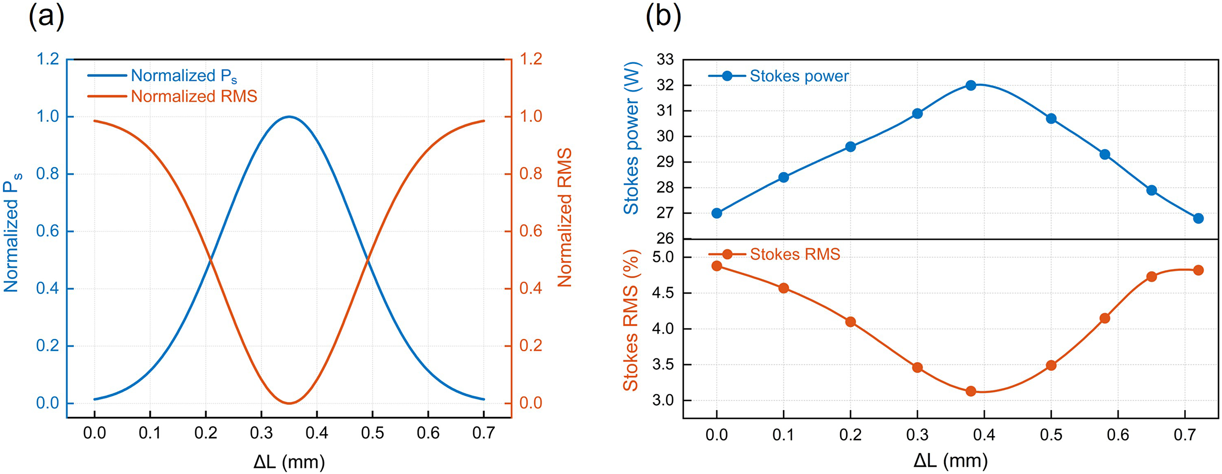
 attains its minimum at the same location. This yields the ‘U-shaped valley’ characteristic seen in Figure 4(a), where the theoretical curve exhibits a minimum power fluctuation sensitivity – a signature of resonance matching. This behavior indicates that the cavity-length offset compensates for the thermally induced shift of the cavity eigenmode. Under this condition, the pump and Stokes modes are optimally matched, and the output becomes least sensitive to small cavity-length perturbations. As a result, the laser simultaneously achieves maximum output power and minimum fluctuation sensitivity.
Output characteristics of the external-cavity diamond Raman laser under different cavity-length compensation values ΔL. (a) Calculated first-order Stokes output power and power stability as functions of ΔL. (b) Measured first-order Stokes output power and power stability as functions of ΔL.

Figure 4 Long description
Panel a is a line graph showing calculated values. The horizontal axis is Delta L in millimeters ranging from 0.0 to 0.7. The left vertical axis is Normalized P sub s in blue and the right vertical axis is Normalized R M S in orange. The Normalized P sub s curve is a bell-shaped peak starting near 0 at Delta L equals 0, peaking at 1.0 when Delta L is approximately 0.35, and returning to near 0 at 0.7. The Normalized R M S curve is an inverted bell shape, starting near 1.0, reaching a minimum of 0 at Delta L equals 0.35, and returning to near 1.0 at 0.7.
Panel b is a line graph showing measured values with data points. The horizontal axis is Delta L in millimeters from 0.0 to 0.7. The top section shows Stokes power in Watts on the vertical axis. The blue data points form a peak, rising from 27 Watts at 0.0 to a maximum of 32 Watts at approximately 0.38, then decreasing to 26.8 Watts at 0.7. The bottom section shows Stokes R M S as a percentage. The orange data points form a trough, starting at 4.9 percent, reaching a minimum of 3.1 percent at Delta L equals 0.38, and rising back to 4.8 percent at 0.7.
3.2 Experimental results of cavity-length compensation
To verify the correctness of the chained model and the PVC criterion, cavity-length compensation experiments were carried out. Figure 4 presents the theoretical calculations and experimental results of the Stokes output power and power stability for different cavity-length compensation values ΔL. As shown in Figure 4(a), theoretical calculations indicate that Ps (ΔL) exhibits a single-peaked profile, whereas RMS(ΔL) follows a characteristic U-shaped curve; the extrema of the two coincide at the same position ΔL*, where the maximum output power and minimum power instability are simultaneously achieved. Here, the optimal cavity-length compensation ΔL* is uniquely defined as the cavity-length offset at which the output power peak and the power stability (RMS) valley coincide. This phenomenon indicates that at this cavity length the pump and Stokes mode fields are optimally matched, yielding the highest intracavity coupling efficiency while minimizing thermally induced phase mismatches.
The experimentally measured results, shown in Figure 4(b), follow the theoretical trend: the output power reaches a maximum of approximately 32 W at ΔL ≈ 0.37 mm, while the power stability improves to RMS ≈ 3.2%. The coincidence of these extrema clearly confirms the PVC rule. These results demonstrate that a simple fine-tuning of the cavity length can compensate for variations in thermal focal length, enabling simultaneous enhancement of output power and stability under high-power operation.
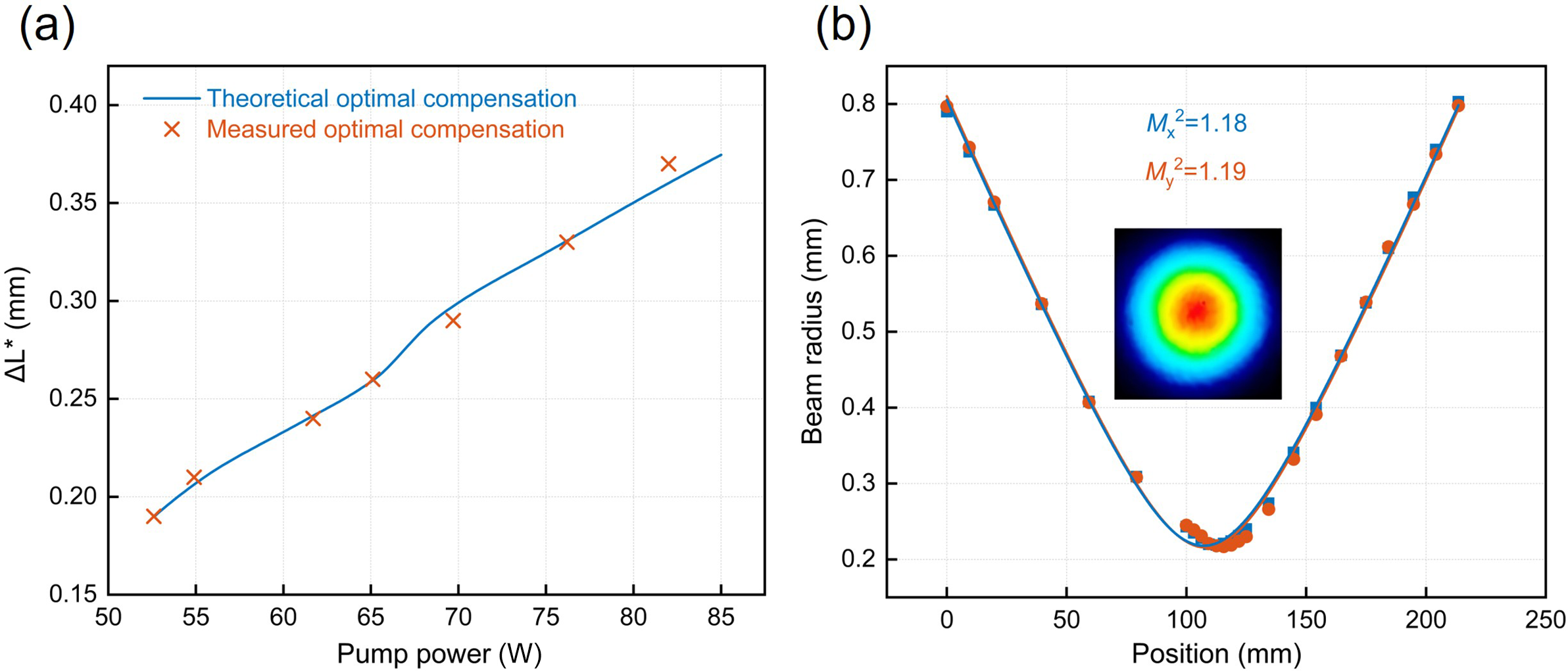
Building on this, the variation of the optimal cavity-length compensation ΔL* under different pump powers was further investigated, and the results are shown in Figure 5(a). The blue solid line represents the model-predicted results, while the orange ‘×’ markers denote the experimentally measured data. It can be seen that the optimal compensation ΔL* increases approximately monotonically with pump power. This trend indicates that increasing pump power enhances the intracavity thermal load and reduces the effective thermal focal length, and thus requires an increase in cavity length to maintain mode-field matching. The theoretical results agree well with the experimental data within the measured power range, with deviations remaining within acceptable limits, thereby confirming the physical soundness and validity of the model. At the maximum investigated pump power of 82 W, after adjusting the cavity length to the optimal compensation value ΔL*, the Stokes output power increased from 27 to 32 W, while the measured beam-quality factors remained near the diffraction limit, with Mx 2 = 1.18 and My 2 = 1.19, as shown in Figure 5(b). Meanwhile, the recorded beam profile retained a near-Gaussian shape. These results indicate that cavity-length compensation enhances output power without introducing significant beam-quality degradation. This behavior agrees with the Raman beam cleanup effect and our coaxial alignment procedure[ Reference Shi, Chen, Gao, Chen, Ding, Wang, Lu and Bai 37 ].
Output characteristics of the first-order Raman laser. (a) Optimal cavity-length compensation ΔL* as a function of pump power, comparing theoretical predictions (blue solid line) with experimental data (orange ‘×’). (b) Beam-quality factors and beam profile of the Stokes output at 82 W after optimal cavity-length compensation.

Figure 5 Long description
Panel a is a line graph. The horizontal x-axis is Pump power in Watts, ranging from 50 to 85. The vertical y-axis is Delta L super asterisk in millimeters, ranging from 0.15 to 0.40. A blue solid line representing Theoretical optimal compensation shows a non-linear increase. Orange cross marks representing Measured optimal compensation closely follow the blue line at data points 53, 55, 62, 65, 70, 76, and 82 Watts.
Panel b is a line graph. The horizontal x-axis is Position in millimeters, ranging from 0 to 250. The vertical y-axis is Beam radius in millimeters, ranging from 0.2 to 0.8. The data forms a symmetric parabolic U-shaped curve with a minimum near 115 millimeters. Blue squares and orange circles represent data for M sub x super 2 equals 1.18 and M sub y super 2 equals 1.19 respectively. At the center of the graph is an inset square image of the beam profile, showing a circular Gaussian distribution with a red core, transitioning outward through yellow and green to a blue perimeter.
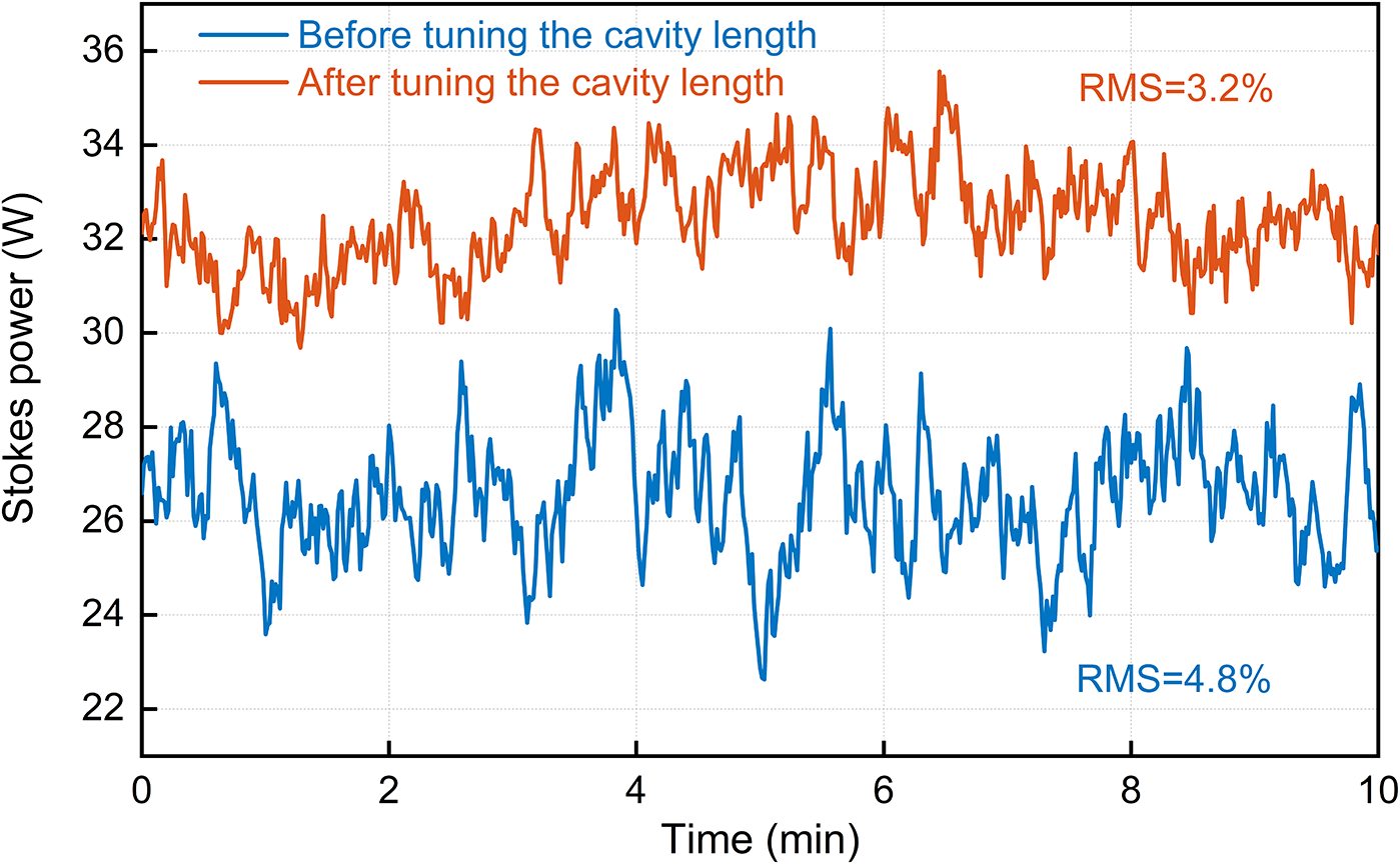
Figure 6 shows the temporal evolution of the Stokes output power before and after applying cavity-length compensation at the maximum output power. The blue curve corresponds to the uncompensated state, while the orange curve represents the result obtained after adjusting the cavity length by the optimal compensation ΔL*. As observed, the uncompensated configuration delivers an average output power of about 27 W with a power fluctuation of RMS ≈ 4.8%; after compensation, the power increases to approximately 32 W and the RMS decreases to 3.2%. The output power increases by roughly 18% and the instability decreases by about 33%, clearly demonstrating that cavity-length adjustment effectively compensates for thermal-focal-length variations and dynamically optimizes mode-field overlap. At this optimal compensation point, the phase curvature of the cavity mode counteracts the phase mismatch induced by the thermal lens, resulting in a more stable optical-field distribution. These results demonstrate that the proposed chained modeling framework and PVC criterion enable steady-state optimal control, providing both theoretical support and experimental validation for the stabilized operation of high-power DRLs. In addition, further improvement in output power and stability may be achievable by enhancing heat-removal efficiency, for example through optimized cooling configurations or improved thermal interface conductivity, which could reduce temperature gradients and suppress thermal-lens fluctuations. From a broader perspective, although demonstrated here in DRLs, the PVC criterion is generally applicable to laser systems in which thermo-optically driven cavity-mode mismatch dominates the performance evolution; in systems where other effects – such as gain saturation, strong nonlinear absorption or multi-mode competition – play a comparable or stronger role than thermal lensing, the PVC behavior may no longer be strictly preserved, and the PVC criterion may require additional constraints or modification.
Comparison of the Stokes output stability before and after optimal cavity-length compensation at a fixed pump power of 82 W. The blue and orange curves correspond to the uncompensated and optimally compensated conditions, respectively.

Figure 6 Long description
The horizontal x-axis represents Time in min, ranging from 0 to 10. The vertical y-axis represents Stokes power in W, ranging from 22 to 36.
Two fluctuating data series are plotted:
* A blue line labeled Before tuning the cavity length fluctuates at a lower power level, primarily between 23 and 30 W. It shows significant instability with a noted R M S equals 4.8%.
* An orange line labeled After tuning the cavity length sits higher on the y-axis, fluctuating between 30 and 36 W. This line exhibits smaller oscillations compared to the blue line, with a noted R M S equals 3.2%.
Both curves show continuous, rapid fluctuations over the ten-minute period, but the orange curve maintains a higher average power and improved stability.
4 Conclusion
In this work, we address the problems of power degradation and output instability in high-power continuous-wave DRLs under strong pumping by developing a chained modeling framework that links the pump power Pp to the cavity-length compensation ΔL. This framework provides a systematic description of the coupled evolution involving optical power, thermal loading and cavity-mode matching. The model identifies thermally induced variations in the effective focal length as the fundamental mechanism responsible for both power reduction and instability, and further establishes an operable PVC criterion. Following this criterion, the cavity length can be used as a single control parameter to simultaneously achieve maximum output power and minimal power fluctuations. Experimental verification confirms both the predictive accuracy and practical applicability of the proposed model. At the theoretically optimized compensation point, the Stokes output power increases from 27 to 32 W, while the RMS instability decreases from 4.8% to 3.2%. These results demonstrate that precise cavity-length tuning alone can effectively compensate for variations in the thermal focal length, enabling a dynamic equilibrium between mode-field overlap and thermally driven effects. Overall, the findings demonstrate that power scaling, thermal management and cavity-mode engineering can be co-optimized within a unified physical framework. The proposed approach provides new modeling tools and physical insights for active steady-state stabilization in high-power solid-state laser systems.
Acknowledgements
This work was supported by the National Key Research and Development Program of China (Grant No. 2024YFE0206000), the National Natural Science Foundation of China (Grant Nos. 62375076 and 61927815), the Natural Science Foundation of Hebei Province (Grant No. F2023202063), the Natural Science Foundation of Tianjin City (Grant No. 22JCYBJC01100), the Natural Science Research Program for Higher Education Institutions in Hebei Province (Grant No. JCZX2025003) and the Science and Technology Cooperation Special Project of Shijiazhuang (Grant No. SJZZXC24006).

 Open access

