2. Mathematical modeling

The derivation of the exact dynamic model of a WIP, as shown in Fig. 2, taking into account movements on the two-dimensional ground surface and two independently driven wheels, can be found in [Reference Zauner, Müller, Gattringer and Jörgl10]. There, no slipping is assumed between the ground and the wheels, thus the WIP can only be moved along the instantaneous ${}_R{x}{}$ -axis, rotated about the ${}_R{z}{}$ -axis, and tilted about the ${}_R{y}{}$ -axis. In order to model these restrictions, non-holonomic constraints at velocity level have to be taken into account. On the contrary, the desired trajectory, adressed in this paper, is guided by a straight line on the ground surface along the ${}_I{x}$ -axis. Therefore, the model can be simplified by setting the orientation angle $\gamma = 0$ and the ${}_I{y}$ -coordinate of the position $y = 0$ . Considering only longitudinal movements, the generalized coordinates $\mathbf{z} = \begin{bmatrix}x & \theta & \xi & \eta \end{bmatrix}^\intercal \hspace{-0.3ex}$ are sufficient to describe the positions and orientations of the basis and the two wheels. The coordinate $x$ describes the position of the ground contact point along the ${}_I{x}$ -axis, $\theta$ is the inclination angle of the basis, and $\xi$ and $\eta$ denote the relative angles of the wheels. Since ideal rolling of the wheels is assumed, the relative angular velocities of the wheels are prescribed by

(1) \begin{equation} \dot{\xi } = \dot{\eta } = \omega _W = \frac{2 \dot{x}}{D_W} - \dot{\theta } \end{equation}

with the diameter of a wheel $D_W$ . Furthermore, the wheels are rotationally symmetric. Consequently, the relative angles of the wheels do not influence the system dynamics and are of no special interest otherwise. Thus it is sufficient to choose the minimal coordinates as $\mathbf{q} = \begin{bmatrix}x & \theta \end{bmatrix}^\intercal \hspace{-0.3ex}$ and accordingly define the minimal velocities by $\dot{\mathbf{s}} = \begin{bmatrix}\dot{x} & \dot{\theta }\end{bmatrix}^\intercal \hspace{-0.3ex}$ . The minimal coordinates and the minimal velocities can then be combined to the vector of states $\mathbf{x} = \begin{bmatrix}\mathbf{q}^\intercal \hspace{-0.3ex} & \dot{\mathbf{s}}^\intercal \hspace{-0.3ex}\end{bmatrix}^\intercal \hspace{-0.3ex}$ . Due to the symmetric structure of the overall robot and the mentioned simplification of the model, the driving torques have to be equal for each wheel. Therefore, the vector of inputs can be stated by $\mathbf{u} = \begin{bmatrix}M\end{bmatrix}$ with $M$ denoting the driving torque for each wheel.

Figure 2. Wheeled inverted pendulum on two-dimensional ground surface.

2.1. Kinematics

Because of $\gamma = 0$ , the reference frames $I$ and $R$ have always the identical orientation and the orientation of the body fixed reference frame $B$ is defined solely by the inclination angle $\theta$ . The rotation matrix

(2) \begin{equation} \mathbf{R}_{BI} = \left[\begin{array}{c@{\quad}c@{\quad}c}\cos \!(\theta ) & 0 & -\sin \!(\theta ) \\ \\[-8pt] 0 & 1 & 0 \\ \\[-8pt] \sin \!(\theta ) & 0 & \cos \!(\theta )\end{array}\right] \end{equation}

can be used to transform vectors represented in frame $I$ , indicated by the left index ${}_I{(\!\cdot\!)}$ , to vectors represented in the frame $B$ , indicated by the left index ${}_B{(\!\cdot\!)}$ . The inverse transformation can be aquired by $\mathbf{R}_{IB} = \mathbf{R}_{BI}^\intercal \hspace{-0.3ex}$ . The angular velocity of the basis and the two wheels are given by

(3) \begin{align}{}_B{\boldsymbol{\omega }}{_{IB}} &={}_I{\boldsymbol{\omega }}{_{IB}} = \begin{bmatrix}0 \\ \\[-8pt] \dot{\theta } \\ \\[-8pt] 0\end{bmatrix}, &{}_I{\boldsymbol{\omega }}{_{IW_1}} &= \begin{bmatrix}0 \\ \\[-8pt] \dot{\xi } + \dot{\theta } \\ \\[-8pt] 0\end{bmatrix} = \begin{bmatrix}0 \\ \\[-8pt] \frac{2 \dot{x}}{D_W} \\ \\[-8pt] 0\end{bmatrix}, &{}_I{\boldsymbol{\omega }}{_{IW_2}} &= \begin{bmatrix}0 \\ \\[-8pt] \dot{\eta } + \dot{\theta } \\ \\[-8pt] 0\end{bmatrix} = \begin{bmatrix}0 \\ \\[-8pt] \frac{2 \dot{x}}{D_W} \\ \\[-8pt] 0\end{bmatrix}, \end{align}

respectively. With the position vectors

(4) \begin{align} {}_I{\mathbf{r}}{_{OG}} &= \begin{bmatrix}x &\quad 0 &\quad 0\end{bmatrix}^\intercal \hspace{-0.3ex}, & {}_I{\mathbf{r}}{_{GP}} &= \begin{bmatrix}0 &\quad 0 &\quad \frac{D_W}{2}\end{bmatrix}^\intercal \hspace{-0.3ex}, &{}_I{\mathbf{r}}{_{OP}} &={}_I{\mathbf{r}}{_{OG}} +{}_I{\mathbf{r}}{_{GP}}, \end{align}

(5) \begin{align}{}_B{\mathbf{r}}{_{PC_B}} &= \begin{bmatrix}c_{B_x} &\quad 0 &\quad c_{B_z}\end{bmatrix}^\intercal \hspace{-0.3ex}, &{}_I{\mathbf{r}}{_{PC_{W_1}}} &= \begin{bmatrix}0 &\quad 0 &\quad c_{W_y}\end{bmatrix}^\intercal \hspace{-0.3ex}, &{}_I{\mathbf{r}}{_{PC_{W_2}}} &= \begin{bmatrix}0 &\quad 0 &\quad -c_{W_y}\end{bmatrix}^\intercal \hspace{-0.3ex}, \end{align}

according to Fig. 2, the velocity vectors for the centers of mass (COM) of the basis and the two wheels $i \in \{1,2\}$ , can be stated by

(6) \begin{align}{}_B{\mathbf{v}}{_{C_B}} &= \mathbf{R}_{BI}{}_I{\dot{\mathbf{r}}}{_{OP}} +{}_B{\dot{\mathbf{r}}}{_{PC_B}} +{}_B{\tilde{\boldsymbol{\omega }}}{_{IB}}{}_B{\mathbf{r}}{_{PC_B}} = \begin{bmatrix} \dot{x} \cos \!(\theta ) + \dot{\theta } c_{B_z} \\ \\[-8pt] 0 \\ \\[-8pt] \dot{x} \sin\! (\theta ) - \dot{\theta } c_{B_x} \end{bmatrix}, \end{align}

(7) \begin{align}{}_I{\mathbf{v}}{_{C_{W_i}}} &={}_I{\dot{\mathbf{r}}}{_{OP}} +{}_I{\dot{\mathbf{r}}}{_{PC_{W_i}}} = \begin{bmatrix}\dot{x} &\quad 0 &\quad 0\end{bmatrix}^\intercal \hspace{-0.3ex}, \end{align}

respectively. Here $\tilde{\boldsymbol{\omega }}$ denotes the skew symmetric cross-product matrix of the vector $\boldsymbol{\omega }$ .

2.2. Dynamics

Based on the definitions in Section 2.1, the momentum vectors for the three bodies are derived by

(8) \begin{align}{}_B{\mathbf{p}}{_{C_B}} &= m_B{}_B{\mathbf{v}}{_{C_B}}, &{}_I{\mathbf{p}}{_{C_{W_i}}} &= m_W{}_I{\mathbf{v}}{_{C_{W_i}}} \end{align}

with the mass of the basis $m_B$ , the mass of a wheel $m_W$ and $i \in \{1,2\}$ . Due to the shape of the basis, the principle axes can be approximated by the axes of the body fixed reference frame $B$ . Therefore, the inertia tensors for the basis and the wheels related to the respective COM can be stated by

(9) \begin{align}{}_B{\mathbf{J}}{_{B}^{C_B}} &= \left[\begin{array}{c@{\quad}c@{\quad}c}J_{B_x} & 0 & 0 \\ \\[-8pt] 0 & J_{B_y} & 0 \\ \\[-8pt] 0 & 0 & J_{B_z}\end{array}\right], &{}_I{\mathbf{J}}{_{W_i}^{C_{W_i}}} &= \left[\begin{array}{c@{\quad}c@{\quad}c}J_{W_r} & 0 & 0 \\ \\[-8pt] 0 & J_{W_a} +{i_G}^2 J_M & 0 \\ \\[-8pt] 0 & 0 & J_{W_r}\end{array}\right], \end{align}

respectively. Thereby the moment of inertia of the drive rotor $J_M$ is transformed to the gear output side with the gear ratio $i_G$ . The vectors of angular momentum can then be defined by

(10) \begin{align}{}_B{\mathbf{L}}{_{C_B}} &={}_B{\mathbf{J}}{_{B}^{C_B}}{}_B{\boldsymbol{\omega }}{_{IB}}, &{}_I{\mathbf{L}}{_{C_{W_i}}} &={}_I{\mathbf{J}}{_{W_i}^{C_{W_i}}}{}_I{\boldsymbol{\omega }}{_{I{W_i}}}. \end{align}

Using the forces due to gravity

(11) \begin{align}{}_B{\mathbf{f}}{_{C_B}^e} &= \mathbf{R}{_{BI}} \begin{bmatrix}0 &\quad 0 &\quad -m_B g\end{bmatrix}^\intercal \hspace{-0.3ex}, &{}_I{\mathbf{f}}{_{C_{W_i}}^e} &= \begin{bmatrix}0 &\quad 0 &\quad -m_W g\end{bmatrix}^\intercal \hspace{-0.3ex}, \end{align}

with the gravitational acceleration $g$ , and the torques due to the motors and viscous friction

(12) \begin{align}{}_B{\mathbf{M}}{_{C_B}^e} &= \mathbf{R}{_{BI}} \left ({}_I{\mathbf{M}}{_{C_{W_1}}^e} +{}_I{\mathbf{M}}{_{C_{W_2}}^e}\right ), &{}_I{\mathbf{M}}{_{C_{W_i}}^e} &= \begin{bmatrix}0 \\ \\[-8pt] M - d_v \left (\frac{2 \dot{x}}{D_W} - \dot{\theta }\right ) \\ \\[-8pt] 0\end{bmatrix}, \end{align}

with the viscous friction coefficient $d_v$ , the reaction forces and torques for the basis and the wheels can be stated by

(13) \begin{align} {}_B{\mathbf{f}}{_{C_B}^z} &={}_B{\dot{\mathbf{p}}}{_{C_B}} +{}_B{\tilde{\boldsymbol{\omega }}}{_{IB}}{}_B{\mathbf{p}}{_{C_B}} -{}_B{\mathbf{f}}{_{C_B}^e}, &{}_I{\mathbf{f}}{_{C_{W_i}}^z} &={}_I{\dot{\mathbf{p}}}{_{C_{W_i}}} -{}_I{\mathbf{f}}{_{C_{W_i}}^e}, \end{align}

(14) \begin{align} {}_B{\mathbf{M}}{_{C_B}^z} &={}_B{\dot{\mathbf{L}}}{_{C_B}} +{}_B{\tilde{\boldsymbol{\omega }}}{_{IB}}{}_B{\mathbf{L}}{_{C_B}} -{}_B{\mathbf{M}}{_{C_B}^e}, &{}_I{\mathbf{M}}{_{C_{W_i}}^z} &={}_I{\dot{\mathbf{L}}}{_{C_{W_i}}} -{}_I{\mathbf{M}}{_{C_{W_i}}^e}, \end{align}

respectively. According to [Reference Bremer12], the equations of motion (EOM) are then determined as

(15) \begin{equation} \begin{bmatrix}\left (\dfrac{\partial {_B{\textbf{v}}_{C_B}}}{\partial \dot{\textbf{s}}}\right )^\intercal \left (\dfrac{\partial {_B{\boldsymbol{\omega}}_{IB}}}{\partial \dot{\textbf{s}}}\right )^\intercal \end{bmatrix} \begin{bmatrix}{}_B{\textbf{f}}{_{C_B}^z} \\ \\[-8pt] {}_B{\textbf{M}}{_{C_B}^z}\end{bmatrix}+ \sum _{i = 1}^2\begin{bmatrix}\left (\dfrac{\partial {_I{\textbf{v}}_{C_{W_i}}}}{\partial \dot{\textbf{s}}}\right )^\intercal \left (\dfrac{\partial {_I{\boldsymbol{\omega}}_{IW_{i}}}}{\partial \dot{\textbf{s}}}\right )^\intercal \end{bmatrix} \begin{bmatrix}{}_I{\textbf{f}}{_{C_{W_i}}^z} \\ \\[-8pt] {}_I{\textbf{M}}{_{C_{W_i}}^z}\end{bmatrix}=\mathbf{0} \end{equation}

By evaluating and rearranging (15), the resulting EOM satisfy the form

(16) \begin{equation} \mathbf{M}(\theta )\ddot{\mathbf{s}} + \mathbf{g}(\theta,\dot{\mathbf{s}}) = \mathbf{B} \mathbf{u} \end{equation}

with the symmetric positive definite mass matrix $\mathbf{M}(\theta )$ , the vector of nonlinear terms $\mathbf{g}(\theta,\dot{\mathbf{s}})$ , and the constant input matrix $\mathbf{B}$ . Since the mass matrix $\mathbf{M}(\theta )$ is invertible, (16) can be converted to state space representation with affine-input structure, resulting in

(17) \begin{equation} \dot{\mathbf{x}} = \begin{bmatrix}\dot{\mathbf{q}} \\ \\[-8pt] \ddot{\mathbf{s}}\end{bmatrix} = \begin{bmatrix}\dot{\mathbf{s}} \\ \\[-8pt] -\mathbf{M}(\theta )^{-1} \mathbf{g}(\theta,\dot{\mathbf{s}})\end{bmatrix} + \begin{bmatrix}\mathbf{0} \\ \\[-8pt] \mathbf{M}(\theta )^{-1} \mathbf{B}\end{bmatrix}\mathbf{u} = \mathbf{f}(\mathbf{x}) + \mathbf{G}(\mathbf{x}) \mathbf{u}. \end{equation}

In order to obtain the equilibrium state of the system, defined by $\dot{\mathbf{s}} = \ddot{\mathbf{s}} = \mathbf{0}$ , the equation system $\mathbf{g}(\theta,\mathbf{0}) = \mathbf{B} \mathbf{u}$ has to be solved. One solution to this equation system is the inclination angle of the upper equilibrium, denoted $\theta _e$ , and the drive torque $M_e = 0$ .

2.3. Ground reaction forces

As mentioned above, the kinematic relation (1) is based on the assumption of ideal rolling of the wheels. In order to ensure that no slipping occurs, the reaction forces between wheels and ground have to stay within static friction bounds. The ground reaction forces/torques, assumed to act at point $G$ for simplicity, can be derived by summing up the reaction forces/torques (13) to (14) properly shifted into point $G$ . This results in

(18) \begin{equation} \begin{bmatrix}{}_I{\mathbf{f}}{_G^z} \\ \\[-8pt]{}_I{\mathbf{M}}{_G^z}\end{bmatrix} = \left[\begin{array}{c@{\quad}c}\mathbf{I} & \mathbf{0} \\ \\[-8pt]{}_I{\tilde{\mathbf{r}}}{_{GC_B}} & \mathbf{I}\end{array}\right]\begin{bmatrix}\mathbf{R}_{IB}{}_B{\mathbf{f}}{_{C_B}^z} \\ \\[-8pt] \mathbf{R}_{IB}{}_B{\mathbf{M}}{_{C_B}^z}\end{bmatrix} + \sum _{i=1}^2 \left[\begin{array}{c@{\quad}c}\mathbf{I} & \mathbf{0} \\ \\[-8pt] {}_I{\tilde{\mathbf{r}}}{_{GC_{W_i}}} & \mathbf{I}\end{array}\right]\begin{bmatrix}{}_I{\mathbf{f}}{_{C_{W_i}}^z} \\ \\[-8pt] {}_I{\mathbf{M}}{_{C_{W_i}}^z}\end{bmatrix} \end{equation}

with ${}_I{\mathbf{r}}{_{GC_B}} ={}_I{\mathbf{r}}{_{GP}} + \mathbf{R}_{IB}{}_B{\mathbf{r}}{_{PC_B}}$ , and ${}_I{\mathbf{r}}{_{GC_{W_i}}} ={}_I{\mathbf{r}}{_{GP}} +{}_I{\mathbf{r}}{_{PC_{W_i}}}$ . As long as the EOM (16) are fulfilled, the ground reaction torques satisfy ${}_I{\mathbf{M}}{_G^z} \equiv \mathbf{0}$ , which can be easily verified by plugging (17) into (18). As expected for the simplified model, the $y$ -component of ${}_I{\mathbf{f}}{_G^z}$ results to $f_{G,y}^z \equiv 0$ . In order to ensure proper ground contact, the $z$ -component has to satisfy the condition

(19) \begin{equation} f_{G,z}^z \ge f_{G,z,\mathrm{min}} \gt 0 \end{equation}

and to ensure ideal rolling the $x$ -component has to be bound by

(20) \begin{equation} -\mu _0 f_{G,z}^z \le f_{G,x}^z \le \mu _0 f_{G,z}^z \end{equation}

with the static friction coefficient $\mu _0$ .

Figure 3. Wheeled inverted pendulum with obstacle.

3. Obstacle avoidance

As can be seen in Fig. 1, the WIP has to get from one side of the obstacle to the other. If only the upper part of the WIP, regarded as the “head,” is considered, three possible outcomes can be observed. First, the head and thus the entire WIP passes under the obstacle and no collision takes place. Second, the head collides directly with the obstacle. And finally, the head passes above the obstacle, which would mean that a different part of the WIP collides with the obstacle. Therefore, it is sufficient to test for collisions between the head and the obstacle, as long as it can be enssured, that the head would not pass above the obstacle. In order to simplify the collision detection between the head and the obstacle, the cross section of the head is approximated, as shown in Fig. 3, by five circles located at the points

(21) \begin{equation}{}_B{\mathbf{r}}{_{PH_i}} = \left[\begin{array}{c}\left (a_{H_1} - \dfrac{h_H}{2}\right ) \dfrac{i - 1}{4} - a_{H_2} \dfrac{5 - i}{4} \\ \\[-8pt] 0 \\ \\[-8pt] H - \dfrac{h_H}{2}\end{array}\right] \end{equation}

with a radius $r_{H_i} = \dfrac{h_H}{2}$ and $i \in \{1,\dots,5\}$ . To account for the sharp edge at the front of the head, the approximation is refined by adding two additional circles at the points

(22) \begin{align}{}_B{\mathbf{r}}{_{PH_6}} &= \begin{bmatrix}a_{H_1} - \dfrac{h_H}{4} &\quad 0 &\quad H - \dfrac{h_H}{4}\end{bmatrix}^\intercal \hspace{-0.3ex}, \end{align}

(23) \begin{align}{}_B{\mathbf{r}}{_{PH_7}} &= \begin{bmatrix}a_{H_1} - \dfrac{h_H}{12} &\quad 0 &\quad H - \dfrac{h_H}{12}\end{bmatrix}^\intercal \hspace{-0.3ex} \end{align}

with the radii $r_{H_6} = \dfrac{h_H}{4}$ and $r_{H_7} = \dfrac{h_H}{12}$ , respectively, and the point

(24) \begin{equation}{}_B{\mathbf{r}}{_{PH_8}} = \begin{bmatrix}a_{H_1} &\quad 0 &\quad H\end{bmatrix}^\intercal \hspace{-0.3ex} \end{equation}

with $r_{H_8} = 0$ for consistency. With the absolute position vectors

(25) \begin{equation}{}_I{\mathbf{r}}{_{OH_i}} ={}_I{\mathbf{r}}{_{OP}} + \mathbf{R}_{IB}{}_B{\mathbf{r}}{_{PH_i}} \end{equation}

with $i \in \{1,\dots,8\}$ and the position vector to the center of the obstacle

(26) \begin{equation}{}_I{\mathbf{r}}{_{OC_O}} = \begin{bmatrix}a_{O_x} & 0 & a_{O_z}\end{bmatrix}^\intercal \hspace{-0.3ex} \end{equation}

the relative position vectors between the head and the obstacle can be stated by

(27) \begin{equation}{}_I{\mathbf{r}}{_{H_iC_O}} ={}_I{\mathbf{r}}{_{OC_O}} -{}_I{\mathbf{r}}{_{OH_i}}. \end{equation}

A noncolliding trajectory always has to satisfy

(28) \begin{equation} \left \Vert{}_I{\mathbf{r}}{_{H_iC_O}}\right \Vert _2 \ge r_{H_i} + r_O \end{equation}

with $i \in \{1,\dots,8\}$ and the radius of the obstacle $r_O$ . In order to ensure that the head does not pass above the obstacle, a test point may never lie inside the triangular shaped region above the center of the obstacle, as indicated in Fig. 3. To achieve this, the condition

(29) \begin{equation} \frac{{}_I{\mathbf{n}}_O^\intercal \hspace{-0.3ex}{}_I{\mathbf{r}}{_{H_iC_O}}}{\left \Vert{}_I{\mathbf{r}}{_{H_iC_O}}\right \Vert _2} \le \cos \!\left (\alpha _{\mathrm{min}}\right ) = \cos \left (\frac{\pi }{6}\right ) = \frac{\sqrt{3}}{2} \end{equation}

with ${}_I{\mathbf{n}}{_O} = \begin{bmatrix}0 &\quad 0 &\quad -1\end{bmatrix}^\intercal \hspace{-0.3ex}$ and $i \in \{1,\dots,8\}$ must always be met.

4. Optimal control problem

4.1. Continuous time domain

Combining the results of Sections 2 and 3, a weighted time and energy optimal trajectory for a fixed obstacle height $a_{O_z}$ can be obtained by solving an OCP with variable terminal time $T_E$ . The according OCP can be stated as

(30) \begin{align} &\! \min _{\mathbf{u}(\cdot),\mathbf{x}(\cdot),T_E}\left ( \nu _t T_E + \nu _u \int _{0}^{T_E} \mathbf{u}(t)^\intercal \hspace{-0.3ex} \mathbf{u}(t) \mathrm{d}{t} \right ) & & & \\[-8pt] \nonumber \end{align}

(31) \begin{align} & \mathrm{s.t.} \quad \frac{\mathrm{d}\boldsymbol{\mathrm{x}} (t)}{\mathrm{d}t} = \mathbf{f}(\mathbf{x}(t)) + \mathbf{G}(\mathbf{x}(t))\mathbf{u}(t) & t & \in [0,T_E] &\\[-8pt] \nonumber \end{align}

(32) \begin{align} & \qquad \ \mathbf{x}(0) = \mathbf{x}_0 & & & \\[-8pt] \nonumber\end{align}

(33) \begin{align} &\qquad\ \mathbf{x}(T_E) = \mathbf{x}_E & & &\\[-8pt] \nonumber\end{align}

(34) \begin{align} &\qquad\ \mathbf{x}_{\mathrm{min}} \le \mathbf{x}(t) \le \mathbf{x}_{\mathrm{max}} & t & \in [0,T_E] &\\[-8pt] \nonumber \end{align}

(35) \begin{align} &\qquad\ \mathbf{u}_{\mathrm{min}} \le \mathbf{u}(t) \le \mathbf{u}_{\mathrm{max}} & t & \in [0,T_E] &\\[-8pt] \nonumber \end{align}

(36) \begin{align}&\qquad\ 0 \lt T_E& & &\\[-8pt] \nonumber \end{align}

(37) \begin{align} &\qquad\ \left |\omega _W(\mathbf{x}(t))\right | \le \omega _{W,\mathrm{max}} & t & \in [0,T_E] & \\[-8pt] \nonumber \end{align}

(38) \begin{align} &\qquad\ \left |P_M(\mathbf{x}(t),\mathbf{u}(t))\right | \le P_{M,\mathrm{max}} & t & \in [0,T_E] &\\[-8pt] \nonumber \end{align}

(39) \begin{align} &\qquad\ f_{G,z,\mathrm{min}}\le f_{G,z}^z(\mathbf{x}(t),\mathbf{u}(t)) & t & \in [0,T_E] & \\[-8pt] \nonumber\end{align}

(40) \begin{align} &\qquad\ \left |f_{G,x}^z(\mathbf{x}(t),\mathbf{u}(t)) \right | \le \mu _0 f_{G,z}^z(\mathbf{x}(t),\mathbf{u}(t)) & t & \in [0,T_E] &\\[-8pt] \nonumber \end{align}

(41) \begin{align} &\qquad\ r_{H_j} + r_O \le \left \Vert{}_I{\mathbf{r}}{_{H_jC_O}}(\mathbf{x}(t))\right \Vert _2 & t & \in [0,T_E],\ j \in \{1,\dots,8\} & \\[-8pt] \nonumber\end{align}

(42) \begin{align} &\qquad\ \frac{{}_I{\mathbf{n}}_O^\intercal \hspace{-0.3ex}{}_I{\mathbf{r}}{_{H_jC_O}}(\mathbf{x}(t))}{\left \Vert{}_I{\mathbf{r}}{_{H_jC_O}}(\mathbf{x}(t))\right \Vert _2} \le \frac{\sqrt{3}}{2} & t & \in [0,T_E],\ j \in \{1,\dots,8\} & \end{align}

with the time weight $\nu _t$ , the input weight $\nu _u$ , the initial state $\mathbf{x}_0 = \begin{bmatrix}0 & \theta _e & 0 & 0\end{bmatrix}$ , and the terminal state $\mathbf{x}_E = \begin{bmatrix}x_E & \theta _e & 0 & 0\end{bmatrix}$ . The vectors $\mathbf{x}_{\mathrm{min}}$ and $\mathbf{x}_{\mathrm{max}}$ form box constraints for the states and are used to restrict especially the inclination angle $\theta$ to reasonable values, whereas the box constraints for the input, given by $\mathbf{u}_{\mathrm{min}}$ and $\mathbf{u}_{\mathrm{max}}$ , account for the maximal permissible driving torque. The angular velocity of the wheels $\omega _W(\mathbf{x})$ , according to (1), is limited to the maximum value $\omega _{W,\mathrm{max}}$ and the drive power $P_{M}(\mathbf{x},\mathbf{u}) = \omega _W(\mathbf{x}) M$ is constrained to the maximal drive power $P_{M,\mathrm{max}}$ . The constraints regarding the ground reaction forces, (39) and (40), are according to (19) and (20) and the constraints concerning obstacle avoidance, (41) and (42), are according to (28) and (29).

4.2. Discrete time domain

To obtain a solution for the infinite-dimensional OCP (30), a direct multiple shooting approach [Reference Bock and Plitt13–Reference Diehl15] is chosen. Therefore, the time span $t \in [0,T_E]$ is discretized with the sampling time $T_S = \frac{T_E}{N}$ , $N = 1000$ , resulting in the vector of time steps $\hat{\mathbf{t}} = \begin{bmatrix}0 & T_S & \cdots & i T_S & \cdots & T_E\end{bmatrix}^\intercal \hspace{-0.3ex} \in \mathbb{R}^{N+1}$ . Between each time step the value of the input vector $\mathbf{u}$ is assumed to be constant. This results in the matrices of discrete input values $\hat{\mathbf{u}} = \begin{bmatrix}\hat{\mathbf{u}}_0 & \hat{\mathbf{u}}_1 & \cdots & \hat{\mathbf{u}}_{N-1}\end{bmatrix} \in \mathbb{R}^{1 \times N}$ and state values $\hat{\mathbf{x}} = \begin{bmatrix}\hat{\mathbf{x}}_0 & \hat{\mathbf{x}}_1 & \cdots & \hat{\mathbf{x}}_N\end{bmatrix} \in \mathbb{R}^{4 \times (N + 1)}$ . As integration scheme the explicit Runge–Kutta method of fourth order RK4 is used, which is implemented explicitly in order to exploit the automatic differentiation capability of the used solver. Consequently, the state of the next time step can be obtained by a function $\mathbf{f}_{\mathrm{RK4}}(\hat{\mathbf{x}}_i, \hat{\mathbf{u}}_i, T_E)$ . The OCP can then be approximated by the finite-dimensional optimization problem

(43) \begin{align} &\min _{\hat{\mathbf{u}},\hat{\mathbf{x}},T_E}\left ( \nu _t T_E + \nu _u \frac{T_E}{N} \sum _{i=0}^{N-1} \hat{\mathbf{u}}_i^\intercal \hspace{-0.3ex} \hat{\mathbf{u}}_i \right ) &&& \\[-10pt] \nonumber\end{align}

(44) \begin{align} & \mathrm{s.t.} \quad \hat{\mathbf{x}}_{i+1} = \mathbf{f}_{\mathrm{RK4}}(\hat{\mathbf{x}}_i, \hat{\mathbf{u}}_i, T_E) & i & \in \{0,\dots,N\} & \\[-10pt] \nonumber \end{align}

(45) \begin{align} &\qquad\ \hat{\mathbf{x}}_0 = \mathbf{x}_0 & & & \\[-10pt] \nonumber \end{align}

(46) \begin{align} & \qquad\ \hat{\mathbf{x}}_N = \mathbf{x}_E & & &\\[-10pt] \nonumber \end{align}

(47) \begin{align} & \qquad\ \mathbf{x}_{\mathrm{min}} \le \hat{\mathbf{x}}_i \le \mathbf{x}_{\mathrm{max}} & i & \in \{0,\dots,N+1\} &\\[-10pt] \nonumber \end{align}

(48) \begin{align} &\qquad\ \mathbf{u}_{\mathrm{min}} \le \hat{\mathbf{u}}_i \le \mathbf{u}_{\mathrm{max}} & i &\in \{0,\dots,N\} & \\[-10pt] \nonumber \end{align}

(49) \begin{align} &\qquad\ 0 \lt T_E & & &\\[-10pt] \nonumber \end{align}

(50) \begin{align} &\qquad\ \left |\omega _W(\hat{\mathbf{x}}_i)\right | \le \omega _{W,\mathrm{max}} & i & \in \{0,\dots,N+1\} &\\[-10pt] \nonumber \end{align}

(51) \begin{align} &\qquad\ \left |P_M(\hat{\mathbf{x}}_i,\hat{\mathbf{u}}_i)\right | \le P_{M,\mathrm{max}} & i & \in \{0,\dots,N\} &\\[-10pt] \nonumber \end{align}

(52) \begin{align} &\qquad\ f_{G,z,\mathrm{min}}\le f_{G,z}^z(\hat{\mathbf{x}}_i,\hat{\mathbf{u}}_i) & i & \in \{0,\dots,N+1\} & \end{align}

(53) \begin{align} & \qquad\ \left |f_{G,x}^z(\hat{\mathbf{x}}_i,\hat{\mathbf{u}}_i) \right | \le \mu _0 f_{G,z}^z(\hat{\mathbf{x}}_i,\hat{\mathbf{u}}_i) & i & \in \{0,\dots,N+1\} &\\[-10pt] \nonumber \end{align}

(54) \begin{align} & \qquad\ r_{H_j} + r_O \le \left \Vert{}_I{\mathbf{r}}{_{H_jC_O}}(\hat{\mathbf{x}}_i)\right \Vert _2 & i & \in \{0,\dots,N+1\},\ j \in \{1,\dots,8\} & \\[-10pt] \nonumber\end{align}

(55) \begin{align} &\qquad\ \frac{{}_I{\mathbf{n}}_O^\intercal \hspace{-0.3ex}{}_I{\mathbf{r}}{_{H_jC_O}}(\hat{\mathbf{x}}_i)}{\left \Vert{}_I{\mathbf{r}}{_{H_jC_O}}(\hat{\mathbf{x}}_i)\right \Vert _2} \le \frac{\sqrt{3}}{2} & i & \in \{0,\dots,N+1\},\ j \in \{1,\dots,8\} & \end{align}

for a fixed obstacle height $a_{O_z}$ . Constraint (44) accounts for the shooting gap between integration of one time step and the optimization varibale of the according next time step.

4.3. Minimal obstacle height

In order to obtain the minimal obstacle height $a_{O_z}$ for which a feasible solution exists, the nested optimization problem

(56) \begin{align} & \min _{\hat{\mathbf{u}},\hat{\mathbf{x}},T_E,a_{O_z}}\left (a_{O_z}\right ) \end{align}

(57) \begin{align} & \mathrm{s.t.} \quad a_{O_z,\mathrm{min}} \le a_{O_z} \end{align}

(58) \begin{align} & \qquad\ (\hat{\mathbf{u}},\hat{\mathbf{x}},T_E) = \arg \min _{\hat{\mathbf{u}},\hat{\mathbf{x}},T_E}\left ( \nu _t T_E + \nu _u \frac{T_E}{N} \sum _{i=0}^{N-1} \hat{\mathbf{u}}_i^\intercal \hspace{-0.3ex} \hat{\mathbf{u}}_i \right ) \\\nonumber &\qquad\ \qquad\ \qquad\ \quad\ \mathrm{s.t.} \quad \text{(44) to (55)} \end{align}

with the discretized OCP as constraint has to be solved. The obstacle height is restricted to reasonable values by $a_{O_z,\mathrm{min}} \gt 0$ , which is chosen in such a way that it does not restrict the actual solution.

5. Numerical solution

For solving the nonlinear optimization problem (43), the optimization framework CasADi [Reference Andersson, Åkesson and Diehl16,Reference Andersson, Gillis, Horn, Rawlings and Diehl17] is used with the solver Ipopt, which is based on [Reference Wächter18]. In order to solve the nested optimization problem (56) a simple line search algorithm can be used for the top-level optimization problem. Thereby the obstacle height $a_{O_z}$ is initialized to some value $a_{O_z} \gt \frac{D_W}{2} + H + r_O$ and then incremenetally reduced by a fixed step size $\Delta{}a_{O_z}$ , which in turn is reduced once no feasible solution for the inner optimization problem can be found. A minimum step size can be used as terminal condition.

To find an initial guess for the inner optimization problem, a straight forward approach would be to linearly interpolate the initial and terminal state and to find a hard lower bound for the terminal time, which is then relaxed by some factor. A reasonable lower bound for $T_E$ can be derived, for example, by the maximum drive speed and the distance between initial and terminal position. The resulting trivial initial guess can be stated as

(59) \begin{align} \hat{\mathbf{x}}_i^{\mathrm{I}_0} &= \frac{N+1-i}{N+1}\mathbf{x}_0 + \frac{i}{N+1}\mathbf{x}_E, & \hat{\mathbf{u}}^{\mathrm{I}_0} &= \mathbf{0}, & T_E^{\mathrm{I}_0} &= 5\frac{2 (x_E-x_0)}{D_W \omega _{W,\mathrm{max}}}. \end{align}

But if this problem is tried to be solved, the optimization process tends to terminate prematurely once the obstacle height reaches $a_{O_z} \lt \frac{D_W}{2} + H + r_O$ . Figure 4 shows the system states of the WIP, for an examplary trajectory, where such a premature termination occurs, and Fig. 5 indicates the resulting trajectory by showing the cross section of the head during motion and the obstacle. Remarkably, the WIP is not tilted at all directly underneath the obstacle, although it is known that a better feasible solution exists.

Figure 4. Premature termination: states over time.

Figure 5. Premature termination: cross section of head during motion.

Since the essence of the desired task is that the WIP has to pass underneath the obstacle, there exists a point in time where the highest point of the WIP has to be below the lowest point of the obstacle. Figure 6 shows the overall height of the WIP for varying inclination angle $\theta$ . It can be seen that there exists a local minimum at $\theta = 0$ , which is caused by the shape of the head. If the initial guess is near this local minimum directly underneath the obstacle, the solver may fail to escape this local infeasible minimum.

Figure 6. WIP overall height.

Of course it is possible to adapt the initial guess or the solver settings such that the optimization process converges more robustly. But this involves tedious handcrafting of initial solutions, which can be avoided by using a multistage approach as proposed in the following section.

6. Multistage approach

The basis for the multistage approach is that the OCP (43) can be solved very robustly, if the constraints regarding the obstacle are neglected. The idea is then to approach the original problem via multiple stages of optimization problems by tightening the constraints and minimizing the obstacle height. Thereby the result of one stage is used as initial guess for the next stage. As a side effect, the minimal obstacle height can also be derived along the way and a higher level line search is no longer necessary.

6.1. Without obstacle

As already mentioned the first stage consists of finding a valid solution for the OCP (43) without the constraints regarding the obstacle. The optimization problem thus simplifies to

(60) \begin{alignat}{2} &\min _{\hat{\mathbf{u}},\hat{\mathbf{x}},T_E}\left ( \nu _t T_E + \nu _u \frac{T_E}{N} \sum _{i=0}^{N-1} \hat{\mathbf{u}}_i^\intercal \hspace{-0.3ex} \hat{\mathbf{u}}_i \right ) \,\, \\\nonumber &\mathrm{s.t.} \quad \text{(44) to (53)} \end{alignat}

Using the trivial initial guess (59), the problem (60) can be solved and the results for the optimization variables $\hat{\mathbf{u}}$ , $\hat{\mathbf{x}}$ , and $T_E$ can be used as initial guess for the next stage. The resulting trajectory is indicated in Fig. 7, which shows the cross section of the head during motion.

Figure 7. Stage 1: cross section of head during motion.

6.2. Head with circular shape and variable obstacle height

In the second stage, the constraints regarding the obstacle are modified in such a way that these constraints no longer have a local minimum at $\theta = 0$ , which has been discussed in Section 5. This can be achieved by using a coarser approximation of the head shape with only one larger circle. To this end, the absolute position vector to the center of the head

(61) \begin{equation}{}_I{\mathbf{r}}{_{OC_H}} ={}_I{\mathbf{r}}{_{OP}} + \mathbf{R}_{IB}{}_B{\mathbf{r}}{_{PC_H}} \end{equation}

with

(62) \begin{equation}{}_B{\mathbf{r}}{_{PC_H}} = \begin{bmatrix}0 & 0 & H - \frac{h_H}{2}\end{bmatrix}^\intercal \hspace{-0.3ex} \end{equation}

is introduced. The relative position vector between the head and the obstacle can then be stated by

(63) \begin{equation}{}_I{\mathbf{r}}{_{C_HC_O}} ={}_I{\mathbf{r}}{_{OC_O}} -{}_I{\mathbf{r}}{_{OC_H}}. \end{equation}

Satisfying the relation

(64) \begin{equation} \left \Vert{}_I{\mathbf{r}}{_{C_HC_O}}\right \Vert _2 \ge r_O + \sqrt{a_{H_1}^2 + \frac{h_H^2}{4}} \end{equation}

leads to a more restrictive constraint, which no longer has a local minimum at $\theta = 0$ .

Furthermore, the height of the obstacle is minimized starting at a height which is known to not interact with the initial guess obtained by the previous stage. The resulting optimization problem can be stated as

(65) \begin{align} &\min _{\hat{\mathbf{u}},\hat{\mathbf{x}},T_E,a_{O_z}}\left ( \nu _t T_E + \nu _u \frac{T_E}{N} \sum _{i=0}^{N-1} \hat{\mathbf{u}}_i^\intercal \hspace{-0.3ex} \hat{\mathbf{u}}_i + \nu _O a_{O_z} \right ) & & & \\\nonumber &\mathrm{s.t.} \quad \text{(44) to (53)} & & & \end{align}

(66) \begin{align} &\qquad\ r_O + \sqrt{a_{H_1}^2 + \frac{h_H^2}{4}} \le \left \Vert{}_I{\mathbf{r}}{_{C_HC_O}}(\hat{\mathbf{x}}_i)\right \Vert _2 & i & \in \{0,\dots,N+1\} & \end{align}

(67) \begin{align} & \qquad\ \frac{{}_I{\mathbf{n}}_O^\intercal \hspace{-0.3ex}{}_I{\mathbf{r}}{_{C_HC_O}}(\hat{\mathbf{x}}_i)}{\left \Vert{}_I{\mathbf{r}}{_{C_HC_O}}(\hat{\mathbf{x}}_i)\right \Vert _2} \le \frac{\sqrt{3}}{2} & i & \in \{0,\dots,N+1\} & \end{align}

(68) \begin{align} &\qquad\ a_{O_z,\mathrm{min}} \le a_{O_z} \end{align}

with the weight $\nu _O \gg \nu _t$ and $\nu _O \gg \nu _u$ . Again the resulting trajectory, which is indicated by Fig. 8 and the detailed view in Fig. 9, can be used as initial guess for the next stage.

Figure 8. Stage 2: cross section of head during motion.

Figure 9. Stage 2: detailed view of obstacle avoidance.

6.3. Head with original shape and variable obstacle height

As can be seen in Fig. 9, the previously introduced coarser approximation of the head shape still leaves a gap between the actual head and the obstacle. In order to further reduce the height of the obstacle and to push the system to its limits, the optimization problem (65) is solved again, but now with the original constraints regarding the obstacle. The according optimization problem is given by

(69) \begin{alignat}{2} &\min _{\hat{\mathbf{u}},\hat{\mathbf{x}},T_E,a_{O_z}}\left ( \nu _t T_E + \nu _u \frac{T_E}{N} \sum _{i=0}^{N-1} \hat{\mathbf{u}}_i^\intercal \hspace{-0.3ex} \hat{\mathbf{u}}_i + \nu _O a_{O_z} \right ) \,\, \\\nonumber &\mathrm{s.t.} \quad \text{(44) to (55) and (68)} \end{alignat}

and Fig. 10 shows that the head now touches but does not intersect the obstacle.

Figure 10. Stage 3: detailed view of obstacle avoidance.

6.4. Original problem

Due to the very high weight for the obstacle height $\nu _O$ the cost functions of the problems, (65) and (69) are significantly different in contrast to the original problem. Therefore in the final stage, the obstacle height is fixed to the result for $a_{O_z}$ of (69) and the original problem (43) is solved using the remaining results of (69) as initial guess.

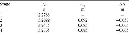
The results of this optimization are shown in Figs. 11–14. Figure 11 depicts the states of the WIP over time. In Fig. 12, it can be seen, that the driving torque and the angular velocity of the wheels, as well as the drive power stay always within the according maximum values (red). The ground reaction forces over time are shown in Fig. 13. Since the actual force ${}_I{f}{_{G,x}^z}$ between the wheels and the ground is always within the limits given by static friction (red), it can be assumed, that no slipping occurs. In Fig. 14, the resulting trajectory is indicated by showing the cross section of the head during motion and the obstacle. The minimal feasible height of the center of the obstacle results in $a_{O_z,\mathrm{opt}} = \mathrm{0.685}\,\mathrm{m}$ . Taking into account the overall height of the WIP of $\mathrm{0.7}\,\mathrm{m}$ and the radius of the obstacle $r_O = \mathrm{0.05}\,\mathrm{m}$ , the lowest point of the obstacle lies $\Delta{}H = -\mathrm{0.065}\,\mathrm{m}$ underneath the highest point of the WIP in the upper equilibrium state. Table I shows how the terminal time and the obstacle height evolve over the four stages.

Figure 11. Optimization result: states over time.

Figure 12. Optimization result: driving torque and angular velocity of the wheels and drive power over time with respect to the according limits (red).

Table I. Resulting terminal time and obstacle height.

Figure 13. Optimization result: ground reaction forces over time with respect to the limits (red).

Figure 14. Optimization result: cross section of head during motion.

Figure 15. Experimental setup: control loop.

7. Experimental setup

In order to test the optimal trajectory on the real system, a linear quadratic regulator (LQR) based approach is used as shown in Fig. 15. A more elaborated controller design would be conceivable, given the nonlinearity of the underlying system. But the optimal trajectory already satisfies the system dynamcis and limits, thus the controller only has to compensate for model uncertainties and measurement errors. The actual system is equipped with encoders and an inertial measurement unit (IMU), providing measurments for the wheel angles $\xi$ and $\eta$ and the inclination angle $\theta$ as well as the respective angular velocities $\dot{\xi }$ , $\dot{\eta }$ , and $\dot{\theta }$ . In order to reduce the measurement noise, especially for the angular velocities, a Kalman observer is added to the control loop. The derivation of the LQR and the observer follows standard procedures and is based on an extended model, which also accounts for lateral deviations off the trajectory. For the extended model, a state vector $\mathbf{x}_{\mathrm{E}} = \begin{bmatrix}\xi & \eta & \theta & \dot{\xi } & \dot{\eta } & \dot{\theta }\end{bmatrix}^\intercal \hspace{-0.3ex}$ and an input vector $\mathbf{u}_{\mathrm{E}} = \begin{bmatrix}M_1 & M_2\end{bmatrix}^\intercal \hspace{-0.3ex}$ are used and the derivation of the EOM is similar to the approach in Section 2. Converting the optimal state values to the desired states of the extended model $\mathbf{x}_{\mathrm{E},\mathrm{des}}$ can be performed by $\xi = \eta = \frac{2 x}{D_W} - \theta$ and (1) and a feedforward for the control input $\mathbf{u}_{\mathrm{E},\mathrm{FF}} = \begin{bmatrix}M_{1,\mathrm{FF}} & M_{2,\mathrm{FF}}\end{bmatrix}^\intercal \hspace{-0.3ex}$ is implemented by setting $M_{1,\mathrm{FF}} = M_{2,\mathrm{FF}} = M$ . The LQR and the observer are based on the extended system dynamics linearized at the upper equilibrium point defined by $\mathbf{x}_{\mathrm{E},\mathrm{equ}} = \begin{bmatrix}0 & 0 & \theta _e & 0 & 0 & 0\end{bmatrix}^\intercal \hspace{-0.3ex}$ and $\mathbf{u}_{\mathrm{E},\mathrm{equ}} = \mathbf{0}$ . This results in the linearized state vector $\boldsymbol{\Delta }\mathbf{x}_{\mathrm{E}} = \mathbf{x}_{\mathrm{E}} - \mathbf{x}_{\mathrm{E},\mathrm{equ}}$ and the linearized input vector $\boldsymbol{\Delta }\mathbf{u}_{\mathrm{E}} = \mathbf{u}_{\mathrm{E}} - \mathbf{u}_{\mathrm{E},\mathrm{equ}}$ . As indicated in Fig. 15, the measured values are collected in $\mathbf{x}_{\mathrm{E},\mathrm{meas}}$ and the observed system state is denoted $\mathbf{x}_{\mathrm{E},\mathrm{obs}}$ with the deviations from the equilibrium point $\boldsymbol{\Delta }\mathbf{x}_{\mathrm{E},\mathrm{meas}}$ and $\boldsymbol{\Delta }\mathbf{x}_{\mathrm{E},\mathrm{obs}}$ , respectively. The control error is defined by $\mathbf{e}_{\mathrm{E},\mathrm{ctrl}} = \mathbf{x}_{\mathrm{E},\mathrm{des}} - \mathbf{x}_{\mathrm{E},\mathrm{obs}}$ and the actual system input results in $\mathbf{u}_{\mathrm{E}} = \mathbf{u}_{\mathrm{E},\mathrm{ctrl}} + \mathbf{u}_{\mathrm{E},\mathrm{FF}}$ with the optimized feedforward $\mathbf{u}_{\mathrm{E},\mathrm{FF}}$ and the output of the controller $\mathbf{u}_{\mathrm{E},\mathrm{ctrl}}$ . Experiments have shown that the proposed controller is capable of keeping the state of the actual WIP close enough to the optimal trajectory, such that a obstacle can be passed without a collision. Thereby the obstacle is installed at the same position, resulted by the optimization problem (69). Unfortunately the controller is implemented on an embedded micro processor board, which does not provide the possibility to track signals. As a partial compensation, the experiment has been put on our YouTube channel and is accessible via [19].