3.1. General considerations for constructing the stresslet of a stick–slip sphere

To use (2.25) for computing the stresslet of a stick–slip sphere, it is more convenient to expand the spatially varying part $f (\boldsymbol {x})$ of the slip length in terms of surface harmonics (Premlata & Wei Reference Premlata and Wei2021). As to concerning how many terms are required to faithfully describe impacts of slip anisotropy on the stresslet, we need an additional rule, which is guided by general considerations, for constructing an anisotropic stresslet.

According to Batchelor (Reference Batchelor1970), the stresslet $\mathcal {S}_{ij}$ of a force-free particle can have two contributions. One is the common contribution from the particle exerted by the straining motion of the ambient fluid under strain rate $E^\infty _{kl}$. The other is an additional contribution, which can emerge when the particle is subject to rotation at rate of $(\varOmega ^\infty _k -\varOmega _k)$ due to an excess couple on the particle. Since $\mathcal {S}_{ij}$ has to be linear in both $E^\infty _{kl}$ and $(\varOmega ^\infty _k -\varOmega _k)$, it can be constructed in the general form:

(3.1)\begin{equation} \mathcal{S}_{ij} = C_{ijkl}E^\infty_{kl} + C_{ijk}(\varOmega^\infty_k -\varOmega_k). \end{equation}

Here $C_{ijkl}$ and $C_{ijk}$ are the geometric tensors depending on the size, shape and orientation of the particle, and both are symmetrical with respect to $i$ and $j$. Here $C_{ijkl}$ is also symmetrical with respect to $k$ and $l$ since it can only be contracted with $E^\infty _{kl}$.

Now consider a Janus sphere that possesses a stick–slip polarity in a preferential direction $d_i$. The geometric tensors in (3.1) can then be constructed below in terms of $d_i$ by satisfying the above-mentioned symmetry classes,

(3.2a)\begin{gather} C_{ijkl} =\alpha_0 \delta_{ik}\delta_{jl} + \alpha_1(d_id_k \delta_{jl}+d_jd_k \delta_{il}) + \alpha_2 d_id_jd_kd_l , \end{gather}

(3.2b)\begin{gather}C_{ijk} = \alpha_3 (\epsilon_{ikm}d_j+ \epsilon_{jkm}d_i)d_m, \end{gather}

with $\alpha _0$, $\alpha _1$, $\alpha _2$ and $\alpha _3$ being the scalar coefficients.

With (3.2), (3.1) becomes

(3.3)\begin{align} \mathcal{S}_{ij} = \alpha_0 E^\infty_{ij} + \alpha_1(d_id_k E^\infty_{kj}+d_jd_k E^\infty_{ki}) + \alpha_2 d_id_jd_kd_l E^\infty_{kl} + \alpha_3 (\epsilon_{ikm}d_j+ \epsilon_{jkm}d_i)d_m (\varOmega^\infty_k -\varOmega_k), \end{align}

which furnishes the general expression for the stresslet of a stick–slip sphere. As in Nir & Acrivos (Reference Nir and Acrivos1973) and Ramachandran & Khair (Reference Ramachandran and Khair2009), this general stresslet expression is made only of $d_pd_q$ and $d_id_jd_kd_l$, although the last term in (3.3) due to rotation is not included in these previous studies. Since $d_pd_q$ can be described by surface quadrupole corresponding to the second surface harmonics (Anderson Reference Anderson1985; Premlata & Wei Reference Premlata and Wei2021), $d_id_jd_kd_l$ can only be captured by a surface hexadecapole, two orders higher than the former. In other words, to describe the stresslet in the form (3.3) it is necessary to keep at least the first four surface harmonics in the harmonics expansion of the slip length, which will be presented in the next subsection.

It is worth mentioning that involving only $d_pd_q$ and $d_id_jd_kd_l$ in the construction of the stresslet (3.3) can be understood using a symmetry argument. This is because they are the only polyadic combinations using $d_i$ that can work with $E_{ij}^\infty$ and $(\varOmega ^\infty _k-\varOmega _k)$ to form a stresslet that is a symmetric second-order tensor. It is thus impossible to use $d_i$ alone to make such a construction. It follows that surface dipole will make no contribution to the stresslet in a linear flow field. That is, if the sphere is half-faced with a dipole only, its stresslet will show no difference than the uniform-slip one.

3.2. Surface spherical harmonics expansion

Following Premlata & Wei (Reference Premlata and Wei2021), we expand the spatially varying slip length $\lambda (\boldsymbol {x})$ as a series of surface spherical harmonics,

(3.4)\begin{equation} \lambda (\boldsymbol{x})=\sum_{m}(a / r)^{m+1} G_{m}[{\cdot}] \boldsymbol{S}_{m}, \end{equation}

where the $m$th-order polyadic $\boldsymbol {S}_{m}$ denotes surface spherical harmonics,

(3.5)\begin{equation} \boldsymbol{S}_{m} \equiv r^{m+1}(\boldsymbol{\nabla} \cdots \boldsymbol{\nabla})^{m}\left(r^{{-}1}\right), \end{equation}

with $G_m$ being the coefficients to form a scalar product with $\boldsymbol {S}_m$ through operator $[{\cdot }]$. As mentioned in § 3.1, it is necessary to keep the terms at least to $m=4$, requiring the following harmonics for determining the stresslet of a stick–slip sphere:

(3.6)\begin{equation} \left. \begin{aligned} S_{0} & =1,\\ S_{1i} & ={-}n_i,\\ S_{2ij} & = 3n_in_j-\delta_{ij},\\ S_{3ijk} & ={-}15 n_in_jn_k + 3(n_i\delta_{jk}+n_j\delta_{ik}+n_k\delta_{ij}),\\ S_{4ijkl} & = 105 n_in_jn_kn_l +3(\delta_{ij}\delta_{kl}+ \delta_{ik}\delta_{jl}+ \delta_{il}\delta_{jk})\\ & \quad -15(n_i n_j \delta_{kl}+n_i n_k \delta_{jl}+ n_i n_l \delta_{jk}+ n_j n_k \delta_{il}+ n_j n_l \delta_{ik}+ n_k n_l \delta_{ij}) . \end{aligned} \right\} \end{equation}

To determine the coefficients $G_m$ in (3.4), the orthogonal relationships between distinct surface harmonics are needed,

(3.7)\begin{equation} \left\langle\boldsymbol{S}_{m} \boldsymbol{S}_{k}\right\rangle=1 /\left( 4 {\rm \pi}a^{2}\right) \int_{S p} \boldsymbol{S}_{m} \boldsymbol{S}_{k} \,\mathrm{d} S, \end{equation}

with $\langle \cdots \rangle = 1 / (4 {\rm \pi}a^{2}) \int _{S_{p}}(\cdots ) \,\mathrm {d} S$ denoting the average over the sphere's surface. The orthogonal relationships for the required surface harmonics (3.6) are given by

(3.8)\begin{equation} \left. \begin{aligned} \left\langle S_{0} S_{0}\right\rangle & =1,\\ \left\langle\boldsymbol{S}_{1} \boldsymbol{S}_{1}\right\rangle_{i j} & =\frac{1}{3} \delta_{i j},\\ \left\langle\boldsymbol{S}_{2} \boldsymbol{S}_{2}\right\rangle_{i j k l} & =\frac{1}{5}\left({-}2 \delta_{i j} \delta_{k l}+3 \delta_{i k} \delta_{j l}+3 \delta_{i l} \delta_{j k}\right), \\ \left\langle\boldsymbol{S}_{3} \boldsymbol{S}_{3}\right\rangle_{i j k pql} & =\frac{15}{7}\left (\delta_{ij}A_{pqkl}+\delta_{ik}A_{pqjl}+\delta_{ip}A_{jklq}+\delta_{iq}A_{jklp}+\delta_{il}A_{jkpq} \right )\\ & \quad -3 \left (\delta_{pq}A_{ijkl}+\delta_{pl}A_{ijkq}+\delta_{ql}A_{ijkp} \right ),\\ \left\langle\boldsymbol{S}_{4} \boldsymbol{S}_{4}\right\rangle_{i j kl pqrs} & =\frac{35}{3}\left[C_{ijklpqrs}+\frac{9}{5}A_{ijkl}A_{pqrs}+ \frac{9}{7}(\delta_{rs}B_{ijklpq}+\delta_{qs}B_{ijklpr}\right.\\ & \quad +\,\delta_{qr}B_{ijklps}+\delta_{ps}B_{ijklqr}+\delta_{pr}B_{ijklqs}+\delta_{pq}B_{ijklrs})\bigg]. \end{aligned} \right\} \end{equation}

In the above, $A_{ijkm} = \delta _{ij}\delta _{km}+\delta _{ik}\delta _{jm}+\delta _{im}\delta _{jk}$, $B_{pqijkm} = \delta _{pq}A_{ijkm}+ \delta _{pi}A_{qjkm}+\delta _{pj}A_{iqkm}+\delta _{pk}A_{ijqm}+\delta _{pm}A_{ijkq}$ and $C_{pqijkmnl} = \delta _{km}B_{pqijnl} + \delta _{kn}B_{pqijml}$ $+ \delta _{kl}B_{pqijnm} + \delta _{kp}B_{mqijnl} + \delta _{kq}B_{pmijnl}$ $+ \delta _{ki}B_{pqmjnl} + \delta _{kj}B_{pqimnl}$.

Applying (3.8) to (3.4) and knowing that monopole $\langle \lambda S_0\rangle =\langle \lambda \rangle (=\hat \lambda )$ is simply the average slip length, we can decompose the slip variation part into a superposition of surface moments by retaining at least the first four ones: dipole $\boldsymbol {P}_{1} \equiv -\langle \lambda \boldsymbol {S}_{1}\rangle ;$ quadrupole $\boldsymbol {P}_{2} \equiv \langle \lambda \boldsymbol {S}_{2}\rangle ;$ octupole $\boldsymbol {P}_{3} \equiv - \langle \lambda \boldsymbol {S}_{3}\rangle$; hexadecapole $\boldsymbol {P}_{4} \equiv \langle \lambda \boldsymbol {S}_{4}\rangle$ etc.: $\lambda ^{\prime }(\boldsymbol {y}) =\langle \lambda \rangle -3 \boldsymbol {P}_{1} \boldsymbol {\cdot} \boldsymbol {S}_{1}+(5 / 6) \boldsymbol {P}_{2}: \boldsymbol {S}_{2}+\cdots,$ etc., giving

(3.9)\begin{equation} \varepsilon f(\boldsymbol{x}) ={-}3P_{1i}S_{1i}+(5/6) P_{2ij}{S}_{2ij}-(7/90) P_{3ijk}{S}_{3ijk}+(1/280) P_{4ijkl} {S}_{4ijkl}+\cdots. \end{equation}

The surface moments $\boldsymbol {P}_1$, $\boldsymbol {P}_2$, $\boldsymbol {P}_3$ and $\boldsymbol {P}_4$ in (3.9) can be written in terms the stick–slip director $\boldsymbol {d}$ with the corresponding strengths $\mathcal {D}$, $\mathcal {Q}$, $\mathcal {O}$ and $\mathcal {H}$:

(3.10a)\begin{align} {P}_{1i} &= \mathcal{D} d_i, \end{align}

(3.10b)\begin{align} {P}_{2ij} &= \mathcal{Q}(3 {d_id_j}-\delta_{ij}), \end{align}

(3.10c)\begin{align} {P}_{3ijk} &= 3{O}(5d_id_jd_k - d_i\delta_{jk}-d_j\delta_{ik}-d_k\delta_{ij}), \end{align}

(3.10d)\begin{align} {P}_{4ijkl} &= 3\mathcal{H} \left[ 35 d_id_jd_kd_l +\delta_{ij}\delta_{lk}+ \delta_{ik}\delta_{jl}+ \delta_{il}\delta_{jk}\right. \nonumber\\&\quad \left.-\,5(d_i d_j \delta_{kl}+d_i d_k \delta_{jl}+ d_i d_l \delta_{jk}+ d_j d_k \delta_{il}+ d_j d_l \delta_{ik}+ d_k d_l \delta_{ij}) \right]. \end{align}

As illustrated in figure 2, the above surface moments represent distinct symmetries of stick–slip patterns. Dipole $\boldsymbol {P}_1$ is the first odd mode. It can be pictured as a half-faced stick–slip pattern characterized by the director $\boldsymbol {d}$ pointing from the stick face to the slip face (with $\mathcal {D} >0$). Quadrupole $\boldsymbol {P}_2$ is the first even mode, representing a symmetric slip–stick–slip (with $\mathcal {Q} >0$) (or stick–slip–stick with $\mathcal {Q} <0$) pattern of striped type. Octupole $\boldsymbol {P}_3$ is the second odd mode, made of two antisymmetric hemispheres with stripes. Hexadecapole $\boldsymbol {P}_4$ is the second even mode, represented by symmetric caps with an alike stripe in the middle.

Figure 2.

Schematic illustrations of the first four surface moments. Dipole $\boldsymbol {P}_1$ can be pictured as a half-faced stick–slip pattern. Quadrupole $\boldsymbol {P}_2$ can be thought of as a symmetric slip–stick–slip ($\mathcal {Q} >0$) or stick–slip–stick $(\mathcal {Q} <0$) pattern of striped type. Octupole $\boldsymbol {P}_3$ can be represented by two antisymmetric hemispheres with stripes. Hexadecapole $\boldsymbol {P}_4$ can be deemed as a pattern possessing symmetric caps with an alike stripe in the middle.

Substitution of (3.9) into (2.25) will allow us to systematically quantify impacts of slip anisotropy on $\mathcal {S}_{ij}$ and $\mathcal {L}_k$ in terms of the surface moments above.

To see how the strengths of surface moments are determined for a given axisymmetric slip length distribution, we rewrite (3.9) in terms of the stick–slip director $\boldsymbol {d}$:

(3.11)\begin{align} \varepsilon f(\boldsymbol{x})={-}3 \mathcal{D} d_i {S}_{1i}+(5/2)\mathcal{Q} d_id_j {S}_{2ij}-(7/6){O} d_id_jd_k S_{3ijk} + (3/8)\mathcal{H} d_id_jd_kd_l S_{4ijkl}+\cdots. \end{align}

In deriving (3.11) we have used the fact that these surface moments are zero when any two indices are identical, namely, $S_{2ij}\delta _{ij}$, $S_{3ijk}\delta _{ij}$ and $S_{4ijkl}\delta _{ij}$ are zero. Also note that $\mathcal {D}$, $\mathcal {Q}$, $\mathcal {O}$ and $\mathcal {H}$ are $O(\varepsilon )$ because of $\varepsilon f(\boldsymbol {x})$ in (3.11).

Equation (3.11) plus $\langle \lambda \rangle$ should be equal to the form by expanding the slip length to a Legendre series:

(3.12)\begin{equation} \lambda({\eta})=a_{0} \mathcal{P}_{0}(\eta)+a_{1} \mathcal{P}_{1}(\eta)+a_{2} \mathcal{P}_{2}(\eta) +a_{3} \mathcal{P}_{3}(\eta)+a_{4} \mathcal{P}_{4}(\eta)+\cdots. \end{equation}

Here ${\rm {\mathcal P}}_0(\eta ) = 1,{\rm {\mathcal P}}_1(\eta ) = \eta ,{\rm {\mathcal P}}_2(\eta ) =$ $(3\eta ^2-1)/2,{\rm {\mathcal P}}_3(\eta ) = (5\eta ^3-3\eta )/2,{\rm {\mathcal P}}_4(\eta )$ $= (35\eta ^4-30\eta ^2 + 3)/8$, etc. are the Legendre polynomials with $\eta =\cos \theta$ in terms of the polar angle $\theta$ with respect to the symmetry axis and the coefficients $a_{n}$ are given by $a_{n}=(n+1 / 2) \int _{-1}^{1} \lambda \mathcal {P}_{n}(\eta ) \,\mathrm {d} \eta$. Comparing (3.12) with (3.11), we can determine the strengths of surface moments in terms of $a_n$ (see Appendix A):

(3.13)\begin{equation} \left\langle\lambda\right\rangle=a_{0} , \mathcal{D}=a_{1} / 3, \mathcal{Q}=a_{2} / 5, {O} = a_3/7 \text{ and } \mathcal{H} = a_4/9. \end{equation}

Take a commonly prepared two-faced Janus sphere having slip lengths $\lambda ^+$ and $\lambda ^-$ as an example (see figure 3). With the aid of (3.13), the strengths of surface moments can be readily found:

(3.14a)\begin{gather} \left\langle\lambda\right\rangle = (1 / 2)(\lambda^{+}+\lambda^{-}-(\lambda^{+}-\lambda^{-})\cos\alpha), \end{gather}

(3.14b)\begin{gather}\mathcal{D} =(1 / 4)(\lambda^{+}-\lambda^{-})\sin ^{2} \alpha, \end{gather}

(3.14c)\begin{gather}\mathcal{Q} = (1 / 4) (\lambda^{+}-\lambda^{-}) \sin ^{2} \alpha \cos \alpha , \end{gather}

(3.14d)\begin{gather}{O} = (1/16) (\lambda^{+}-\lambda^{-}) \sin^2 \alpha ( 5 \cos^2 \alpha -1), \end{gather}

(3.14e)\begin{gather}\mathcal{H} = (1/16) (\lambda^{+}-\lambda^{-}) \sin^2 \alpha \cos\alpha (7 \cos^2 \alpha -3), \end{gather}

where $\alpha$ is the stick–slip division angle for the more slippery $\lambda ^{+}$ part. As indicated by (3.14), the strengths of these surface moments are proportional to the stick–slip contrast $(\lambda ^{+}-\lambda ^{-})$ modulated by the stick–slip division angle $\alpha$.

Figure 3.

The slip length distribution of a stick–slip Janus sphere can be represented by its average slip length plus a linear combination of various surface moments listed in figure 2.

4.1. Stresslet

Here we merely present the end results after evaluating the stresslet using (2.25a,b). The detailed evaluations of relevant contributions to the stresslet can be found in Appendix B. The surface monopole measures the average slip length. The associated stresslet is represented by the uniform-slip part (2.25a), which gives

(4.4)\begin{equation} \mathcal{S}^{(0)}_{ij} = \frac{20}{3}\left ( \frac{1+2\hat\lambda}{1+5\hat\lambda} \right ) {\rm \pi}\mu a^3 E^\infty_{ij}\big|_0 +\frac{2}{3}\left ( \frac{1}{1+5\hat\lambda} \right ) {\rm \pi}\mu a^5\nabla^2E^\infty_{ij}\big|_0, \end{equation}

which recovers the result obtained by Keh & Chen (Reference Keh and Chen1996) for a uniform-slip sphere.

The $O(\varepsilon )$ slip anisotropy correction (2.25b) comprises surface dipole, quadrupole, octupole and hexadecapole contributions, $\mathcal {S}^{(1)}_{ij} = \mathcal {S}^D_{ij} + \mathcal {S}^Q_{ij}+ \mathcal {S}^O_{ij}+\mathcal {S}^H_{ij}$, modifying the stresslet according to

(4.5a)\begin{align} \mathcal{S}^D_{ij} &={-} 3a \langle \lambda S_{1k}\rangle {\int_{S_p}} S_{1k} \varSigma^\parallel_{mij} ( - p^\infty {(0)}n_m + x_p \boldsymbol{\nabla}_p\sigma^\infty_{ml}\big|_0n_l +\cdots)\,\mathrm{d}S \nonumber\\ &={-}\frac{40/7}{1+5\hat\lambda} {\rm \pi}\mu a^4 \;\left (1+\frac{7a^2}{90}\nabla^2\right) \boldsymbol{\nabla}_kE^\infty_{ij}\big|_0 P_{1k} \nonumber\\ &\quad -\frac{12/7}{1+5\hat\lambda} {\rm \pi}\mu a^4 P_{1k} \left[\vphantom{\frac{4}{3}}\boldsymbol{\nabla}_i E^\infty_{jk} \big|_0 + \boldsymbol{\nabla}_j E^\infty_{ik} \big|_0 + \boldsymbol{\nabla}_m E^\infty_{jm} \big|_0 \delta_{ik} + \boldsymbol{\nabla}_m E^\infty_{im} \big|_0 \delta_{jk}\right.\nonumber\\ &\left.\quad -\,\frac{4}{3}\delta_{ij} \boldsymbol{\nabla}_l E^\infty_{lk} \big|_0 \right],\\ \mathcal{S}^{Q}_{ij} &={-} {a} (5/6)\langle \lambda S_{2pq}\rangle\left[ \mu {\int_{S_p}} S_{2pq} \varSigma^\parallel_{mij}\varSigma_{mlk}\; E^\infty_{lk}(0)\,\mathrm{d}S \right. \nonumber\\ &\quad + \mu {\int_{S_p}} S_{2pq}\; \varSigma^\parallel_{mij} R_{mn}\epsilon_{rsn} x_s (\varOmega_{r}^\infty(0)-\varOmega_r)\,\mathrm{d}S \nonumber\\ &\quad +\left.{\int_{S_p}} S_{2pq} \; \varSigma^\parallel_{mij} ( - p^\infty {(0)} n_m + \frac{x_nx_k}{2!}\boldsymbol{\nabla}_n\boldsymbol{\nabla}_k\sigma^\infty_{ml}\big|_0 n_l ) \,\mathrm{d}S \right] \nonumber\\ &={-}\frac{50/7}{(1+5\hat\lambda)^2} {\rm \pi}\mu a^3 \left [E^\infty_{jp}\big|_0 P_{2ip} +E^\infty_{ip}\big|_0 P_{2jp} - \frac{2}{3}\delta_{ij} E^\infty_{pq}\big|_0 P_{2pq} \right ]\nonumber\\ &\quad -\frac{10}{(1+3\hat\lambda)(1+5\hat\lambda)} \; {\rm \pi}\mu a^3 \left[ \epsilon_{irp} P_{2jp} + \epsilon_{jrp} P_{2ip}\right] (\varOmega_{r}^\infty(0)-\varOmega_r) \nonumber\\ &\quad - \frac{20/189}{1+5\hat\lambda} {\rm \pi}\mu a^5 P_{2pq}\bigg[ 5\boldsymbol{\nabla}_p\boldsymbol{\nabla}_k(E^\infty_{jq}\big|_0\delta_{ik}+E^\infty_{iq}\big|_0\delta_{jk})+3\nabla^2 \left(E^\infty_{jq}\big|_0\delta_{ip} + E^\infty_{iq}\big|_0\delta_{jp} \right ) \nonumber\\ &\quad -3\nabla^2E^\infty_{pq}\big|_0\delta_{ij}-2\boldsymbol{\nabla}_i\boldsymbol{\nabla}_j E^\infty_{pq}\big|_0+ 7 \boldsymbol{\nabla}_p\boldsymbol{\nabla}_q E^\infty_{ij}\big|_0\bigg],\\ \mathcal{S}^O_{ij} &={-}a (7/90)\langle \lambda S_{3kpq}\rangle {\int_{S_p}} S_{3kpq} \varSigma^\parallel_{mij} ( - p^\infty (0)\;n_m + x_n \boldsymbol{\nabla}_n\sigma^\infty_{ml}\big|_0\;n_l+\cdots ) \,\mathrm{d}S \nonumber\\ &= {-}\frac{8/27}{1\!+\!5\hat\lambda}\mu {\rm \pi}a^4 \bigg[2\boldsymbol{\nabla}_k E^\infty_{nk} \big|_0 P_{3ijn}\!+\! \delta_{ij} \boldsymbol{\nabla}_l E^\infty_{mn}\big|_0 P_{3mnl} \!+\!\boldsymbol{\nabla}_j E^\infty_{mn}\big|_0 P_{3imn}\!+\!\boldsymbol{\nabla}_i E^\infty_{mn}\big|_0 P_{3jmn} \nonumber\\ &\quad - \frac{5}{2}(\boldsymbol{\nabla}_n E^\infty_{jm}\big|_0 P_{3imn} +\boldsymbol{\nabla}_n E^\infty_{im} \big|_0 P_{3jmn})\bigg], \end{align}

(4.5b)\begin{align} \mathcal{S}^{H}_{ij} &={-} {a}\mu (1/280) \left\langle\lambda S_{4pqrs}\right\rangle {\int_{S_p}} {S}_{4pqrs}\; \varSigma^\parallel_{mij}\varSigma_{mlk}\; E^\infty_{lk}(0) \,\mathrm{d}S \nonumber\\ &=\frac{20/21}{(1+5\hat\lambda)^2}{\rm \pi} \mu a^3 P_{4ijlk}E^\infty_{lk}(0). \end{align}

Note that the stresslet–rotation coupling $(\varOmega _{r}^\infty (0)-\varOmega _r)$ term comes from $\mathcal {S}_{ij}^Q$in (4.5b). Combining (4.4)–(4.5) gives the extended Faxén stresslet relation,

(4.6a)\begin{equation} \mathcal{S}_{ij} = \frac{20}{3} {\rm \pi}\mu a^3 \left( \frac{1+2\hat\lambda}{1+5\hat\lambda} \right) \left [1+ \frac{a^2}{10(1+2\hat\lambda)} \nabla^2 \right] E^\infty_{ij}\big|_0 + {\rm \pi}\mu a^3 J_{3ij} +{\rm \pi} \mu a^4 J_{4ij}+{\rm \pi} \mu a^5 J_{5ij}, \end{equation}

where various finite-size anisotropic contributions from surface moments can be summed up below according to their associations with different powers of $a$:

(4.6b)\begin{align} \displaystyle J_{3ij} &=\frac{20/21}{(1+5\hat\lambda)^2} P_{4ijkl}E^\infty_{kl}\big|_0 \nonumber\\ &\quad -\displaystyle \frac{10}{(1+3\hat\lambda)(1+5\hat\lambda)} P_{2pq} \left[\delta_{jq} \epsilon_{irp} + \delta_{iq} \epsilon_{jrp} \right] (\varOmega_{r}^\infty(0)-\varOmega_r) \nonumber\\ &\quad - \displaystyle \frac{50/7}{(1+5\hat\lambda)^2} P_{2pq}\left [\delta_{iq}E^\infty_{jp}\big|_0 +\delta_{jq}E^\infty_{ip}\big|_0 - \frac{2}{3}E^\infty_{pq}\big|_0\delta_{ij}\right],\end{align}

(4.6c)\begin{align} \displaystyle J_{4ij} &={-}\frac{40/7}{1+5\hat\lambda} P_{1k}\boldsymbol{\nabla}_kE^\infty_{ij} \nonumber\\ &\quad -\frac{12/7}{1+5\hat\lambda} P_{1k} \left[ \boldsymbol{\nabla}_i E^\infty_{jk} \big|_0 + \boldsymbol{\nabla}_j E^\infty_{ik} \big|_0 +\delta_{ik} \boldsymbol{\nabla}_m E^\infty_{jm} \big|_0 + \delta_{jk} \boldsymbol{\nabla}_m E^\infty_{im} \big|_0 -\frac{4}{3}\delta_{ij} \boldsymbol{\nabla}_m E^\infty_{mk} \big|_0 \right] \nonumber\\ &\quad -\frac{8/27}{1+5\hat\lambda} P_{3mnl}\,\bigg[ \frac{5}{2}\boldsymbol{\nabla}_l( E^\infty_{jm}\big|_0 \delta_{in} + E^\infty_{im}\big|_0 \delta_{jn} -\frac{2}{5}E^\infty_{mn}\big|_0 \delta_{ij} ) -( \boldsymbol{\nabla}_j E^\infty_{mn} \big|_0 \delta_{il} \nonumber\\ &\quad +\boldsymbol{\nabla}_i E^\infty_{mn}\big|_0 \delta_{jl}) -2\boldsymbol{\nabla}_k E^\infty_{lk}\big|_0 \delta_{in}\delta_{jm} \bigg] ,\\ J_{5ij}&={-} \frac{20/189}{1+5\hat\lambda} P_{2pq}\,\bigg [ 5\boldsymbol{\nabla}_p(\boldsymbol{\nabla}_iE^\infty_{jq}\big|_0+\boldsymbol{\nabla}_jE^\infty_{iq}\big|_0)+ 3\nabla^2 \left(E^\infty_{jq}\big|_0\delta_{ip} + E^\infty_{iq}\big|_0\delta_{jp} \right ) \nonumber\\ &\quad -3\nabla^2E_{pq}^\infty\big|_0\delta_{ij}-2\boldsymbol{\nabla}_i\boldsymbol{\nabla}_j E^\infty_{pq}\big|_0 + 7\boldsymbol{\nabla}_p\boldsymbol{\nabla}_q E^\infty_{ij}\big|_0\bigg ]. \end{align}

Here a variety of anisotropic stresslet contributions ((4.6b)–(4.6d)) are written in the traceless form to ensure the total stresslet (4.6a) is trace-free. As indicated by (4.6a), in a linear flow field the impacts of slip anisotropy on the stresslet are reflected purely by symmetric quadrupole $\boldsymbol {P}_2$ and hexadecapole $\boldsymbol {P}_4$. The Faxén corrections with the $a^5$ terms also come from these symmetric surface moments when the imposed flow is of a cubic type or of a higher degree. Antisymmetric dipole $\boldsymbol {P}_1$ and octupole $\boldsymbol {P}_3$ affect the stresslet through the finite-size $a^4$ terms if the imposed strain rate is non-uniform.

While the variety of terms associated with distinct surface moments in (4.6b)–(4.6d) may look complicated, each in fact takes a unique and specific form as computed. They can be obtained below using simple tensor constructions guided by the linearity of Stokes flow. For simplicity, we only present canonical forms in the constructions by omitting the associated symmetric parts which can be easy to obtain by interchanging the indices.

First consider the contributions from even surface moments. For quadrupole $P_{2ik}$, constructing a stresslet $\mathcal {S}_{ij}$ with $P_{2ik}$ in a purely straining field $E_{kj}^\infty$ can only be done with $\mathcal {S}_{ij} = P_{2ik} E_{kj}^\infty$. Similarly, that in a purely rotating field $\varOmega ^\infty _r$ can only be constructed as $\epsilon _{jrk}P_{2ik}\varOmega _r^\infty$. These contributions can be seen in (4.6b). As for the Faxén stresslet corrections due to $P_{2ik}$, the admissible forms can only be $P_{2ik}\nabla ^2E^\infty _{jk}$ and $P_{2lk}\boldsymbol {\nabla }_l\boldsymbol {\nabla }_i E^\infty _{jk}$, by having $P_{2ik}E^\infty _{kj}$ operated under differential operators, as obtained in (4.6d). For hexadecapole ${P}_{4ijkl}$, $\mathcal {S}_{ij}$ can only be made in the form of $P_{4ijkl}E_{kl}^\infty$, as shown in (4.6b).

For the contributions from odd surface moments, dipole $P_{1k}$ cannot work with a strain field $E_{ij}^\infty$ but with a field gradient $\boldsymbol {\nabla }_kE_{ij}^\infty$ to yield a stresslet $P_{1k}\boldsymbol {\nabla }_kE_{ij}^\infty$ or $P_{1k}\boldsymbol {\nabla }_iE_{jk}^\infty$, as derived in (4.6c). Similarly, octupole $P_{3ilk}$ can make a contribution $P_{3ilk}\boldsymbol {\nabla }_kE_{jl}^\infty$, $P_{3ijk}\boldsymbol {\nabla }_lE_{lk}^\infty$ or $\boldsymbol {\nabla }_j P_{3ilk}E_{lk}^\infty$ to $\mathcal {S}_{ij}$ when it joins a field gradient $\boldsymbol {\nabla }_kE_{ij}^\infty$ or $\boldsymbol {\nabla }_lE_{lk}^\infty$, as obtained in (4.6c).

Now return to the total stresslet (4.6a). Since (4.6a) contains both the $O(\varepsilon )$ slip anisotropy corrections and the finite-size correction terms of $O((a/L)^2)$ and smaller (with $L$ being the macroscopic length over which flow gradients occur), the former can be more important than the latter if the imposed flow is linear or

(4.7)\begin{equation} \varepsilon\gg (a/L)^2. \end{equation}

Under the above condition, we can neglect the finite-size correction terms $\nabla ^2 \boldsymbol {E}^{\infty }|_0$, $\boldsymbol {P}_1 \boldsymbol {\cdot} \boldsymbol {\nabla } \boldsymbol {E}^\infty |_0$ , $\boldsymbol {\nabla } (\boldsymbol {E}^\infty |_0 \boldsymbol {\cdot} \boldsymbol {P}_1)$, $\boldsymbol {P}_{2}: \boldsymbol {\nabla }\boldsymbol {\nabla } \boldsymbol {E}^\infty |_0$, ${\nabla }^2 \boldsymbol {E}^\infty |_0 \boldsymbol {\cdot} \boldsymbol {P}_{2}$, $\boldsymbol {\nabla } \boldsymbol {\cdot}(\boldsymbol {P}_3\boldsymbol {\cdot} \boldsymbol {E}^\infty |_0)$, $\boldsymbol {P}_3\boldsymbol {\cdot} (\boldsymbol {\nabla }\boldsymbol {\cdot} \boldsymbol {E}^\infty |_0)$, $\boldsymbol {\nabla }(\boldsymbol {P}_3:\boldsymbol {E}^\infty |_0)$ due to the non-uniformity of the imposed strain field, simplifying (4.6a) to

(4.8)\begin{gather} \frac{\mathcal{S}_{ij}}{{\rm \pi} \mu a^3} = \frac{20}{3} \left( \frac{1+2\hat\lambda}{1+5\hat\lambda} \right) E^\infty_{ij}\big|_0 -\frac{50/7}{(1+5\hat\lambda)^2} \left [ P_{2ip}E^\infty_{jp}\big|_0 +P_{2jp}E^\infty_{ip}\big|_0 - (2/3)P_{2pq}E^\infty_{pq}\big|_0\delta_{ij}\right ] \nonumber\\ +\,\frac{{20}/{21}}{(1+5\hat\lambda)^2} P_{4ijlk}E^\infty_{lk}\big|_0 -\frac{10}{(1+3\hat\lambda)(1+5\hat\lambda)}[\epsilon_{irp} P_{2jp} + \epsilon_{jrp} P_{2ip}] (\varOmega_{r}^\infty(0)-\varOmega_r). \end{gather}

It is exactly the general stresslet expression (3.3) when writing quadrupole $P_{2pq}$ and hexadecapole $P_{4ijlk}$ back to $d_pd_q$ and $d_id_jd_ld_k$ using (3.10b) and (3.10d), as can be seen from (5.4) later.

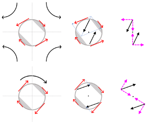
Equation (4.8) reveals that the anisotropic part of stresslet in a linear flow field is determined purely from symmetric $P_{2pq}$ and $P_{4ijlk}$. Note that while these two surface moments contribute to the stresslet in a purely straining field, stresslet–rotation coupling arises only from $P_{2pq}$. In figure 4 we use a slip–stick–slip sphere whose stick–slip pattern can be represented by $P_{2pq}$ to illustrate how stresslets are generated from asymmetric forces around the sphere in linear flow fields. Figure 4(b,c) display how these forces turn into a stresslet and a couple under the actions of a purely straining flow field and those of a purely rotating flow field, respectively. In the latter case, a stresslet can result from the vorticity of an imposed flow or from body rotation, giving rise to the stresslet–rotation coupling term in (4.8) (figure 4c). Likewise, a couple can be generated by applying a strain field to the sphere, resulting in torque-strain coupling (figure 4b). Compared with the usual no-slip case (figure 4a), the main difference is that asymmetric forces on the sphere lead the resulting force pair to be unaligned with respect to the sphere's centre, acting as a symmetric stresslet and an antisymmetric couple across the sphere.

Figure 4.

Schematic cartoons showing the use of a slip–stick–slip sphere for illustrating how different anisotropic stresslet contributions form due to surface quadrupole in a linear flow field in comparison with the usual no-slip case (a). Panel (b) illustrates the situation in a purely straining flow field, showing how asymmetric forces (red arrows) form around the sphere due to the slip asymmetry. These forces then produce a force pair that acts as a symmetric stresslet and an antisymmetric couple across the sphere. The couple is responsible for the torque-strain coupling term in (4.12). Panel (c) displays the similar situation in a purely rotating flow field, explaining how the stresslet–rotation coupling term in (4.8) arises from the vorticity of an imposed flow or from body rotation.

For a Janus sphere whose stick–slip pattern is purely antisymmetric like an equally divided face represented by dipole $P_{1k}$, slip anisotropy will make no contribution to the stresslet until $O(\varepsilon ^2)$. The anisotropic stresslet of such sphere can only be seen by placing the sphere in a nonlinear flow field in which the $a^4$ terms in (4.6a) can emerge due to antisymmetric dipole $P_{1k}$ or/and octupole $P_{3kpq}$.

4.2. Torque

As indicated by (4.6a), the stresslet of a stick–slip sphere can further couple to its rotational motion. To find the rate of rotation for the sphere, we need to determine the hydrodynamic torque on the sphere. Again, we present the end results by leaving the detailed derivations to Appendix C. The uniform-slip part (2.25c) of the torque is

(4.9)\begin{equation} \mathcal{L}_k^{(0)}= \frac{8}{1+3\hat\lambda} {\rm \pi}\mu a^3 (\varOmega_{k}^\infty(0)-\varOmega_k), \end{equation}

which again agrees with the result obtained by Keh & Chen (Reference Keh and Chen1996) for a uniform-slip sphere. Similar to the stresslet (4.6a), the slip anisotropy correction (2.25d) is found to consist of surface dipole, quadrupole and octupole contributions, $\mathcal {L}^{(1)}_{k} = \mathcal {L}^D_{k} + \mathcal {L}^Q_{k}+ \mathcal {L}^O_{k}$, as computed as follows:

(4.10a)\begin{align} \mathcal{L}^D_k &={-} 3{a}\langle \lambda S_{1j} \rangle {\int_{S_p}} S_{1j} \epsilon_{kln}x_l R^\parallel_{mn} ( - p^\infty {(0)}\;n_m + x_p\boldsymbol{\nabla}_p\sigma^\infty_{mq}(0)\;n_q+\cdots )\mathrm{d}S \nonumber\\ &={-}\frac{24/5}{1+3\hat\lambda}{\rm \pi} \mu a^4 \epsilon_{kmn}( \boldsymbol{\nabla}_m E_{jn}^\infty\big|_0 P_{1j} -\boldsymbol{\nabla}_p E^\infty_{pm}\big|_0 P_{1n}), \end{align}

(4.10b)\begin{align} \mathcal{L}^{Q}_k &={-}{a} (5/6)\langle \lambda S_{2ij} \rangle \left[ {\int_{S_p}} S_{2ij} \epsilon_{kln}x_l R^\parallel_{mn} \varSigma_{mpq} E_{pq}^\infty (0) \,\mathrm{d}S \right. \nonumber\\ &\quad +\mu {\int_{S_p}} S_{2ij} \epsilon_{kln}\epsilon_{rsq}x_l x_s R^\parallel_{mn} R_{mq} (\varOmega_{r}^\infty(0)-\varOmega_r )\,\mathrm{d}S \nonumber\\ &\quad +\left. {\int_{S_p}} S_{2ij} \epsilon_{kln}x_l\;R^\parallel_{mn}( - p^\infty{(0)}n_m + \frac{x_p x_q}{2!}\boldsymbol{\nabla}_p\boldsymbol{\nabla}_q\sigma^\infty_{mr}\big|_0n_r +\cdots)\,\mathrm{d}S \right] \nonumber\\ &={-}\frac{20}{(1+3\hat\lambda)(1+5\hat\lambda)}{\rm \pi} \mu a^3 \epsilon_{kmn}P_{2mj} E_{jn}^\infty(0) +\frac{12}{(1+3\hat\lambda)^2}{\rm \pi} \mu a^3 P_{2pk}(\varOmega_{p}^\infty(0)-\varOmega_p ) \nonumber\\ &\quad -\frac{8/7}{1+3\hat\lambda}{\rm \pi} \mu a^5 \epsilon_{klm} \left[- \boldsymbol{\nabla}_j\boldsymbol{\nabla}_p E^\infty_{pl}\big|_{0}P_{2mj} + \boldsymbol{\nabla}_j\boldsymbol{\nabla}_l E^\infty_{mq}\big|_{0} P_{2jq} + (1/2) {\nabla}^2E^\infty_{mq}\big|_{0} P_{2lq}\right ], \end{align}

(4.10c)\begin{align}\mathcal{L}^{O}_k&={-}{a} (7/90)\langle \lambda S_{3pij} \rangle {\int_{S_p}} S_{3pij} \epsilon_{kln}x_l R^\parallel_{mn} ( - p^\infty{(0)} n_m + x_q\boldsymbol{\nabla}_q\sigma^\infty_{mr}(0)\;n_r +\cdots)\,\mathrm{d}S \nonumber\\ &={-}\frac{8/5}{(1+3\hat\lambda)} {\rm \pi}\mu a^4 \epsilon_{kln} \boldsymbol{\nabla}_q E_{mn}^\infty\big|_0 P_{3lmq}. \end{align}

Note that the torque-strain coupling term $\epsilon _{kmn}P_{2mj} E_{jn}^\infty (0)$ comes from $\mathcal {L}^{Q}_k$ in (4.10b) due to the quadrupole. Combining (4.9) and (4.10) yields the extended Faxén relation for the torque:

(4.11)\begin{align} \mathcal{L}_k &= \frac{8}{1+3\hat\lambda} {\rm \pi}\mu a^3 \left[ \delta_{pk}+\frac{3/2}{1+3\hat\lambda}P_{2pk}\right] (\varOmega_{p}^\infty(0)-\varOmega_p ) \nonumber\\ &\quad -\frac{20}{(1+3\hat\lambda)(1+5\hat\lambda)}{\rm \pi} \mu a^3 \epsilon_{kmn}P_{2mj} E_{jn}^\infty(0) \nonumber\\ &\quad -\frac{24/5}{1+3\hat\lambda}{\rm \pi} \mu a^4 \epsilon_{kmn}( \boldsymbol{\nabla}_m E_{jn}^\infty \big|_0 P_{1j} -\boldsymbol{\nabla}_p E^\infty_{pm}\big|_0 P_{1n}) \nonumber \\ &\quad -\frac{8/5}{(1+3\hat\lambda)} {\rm \pi}\mu a^4 \epsilon_{kln} \boldsymbol{\nabla}_q E_{mn}^\infty\big|_0 P_{3lmq} \nonumber\\ &\quad -\frac{8/7}{1+3\hat\lambda}{\rm \pi} \mu a^5 \epsilon_{kln} \left[- \boldsymbol{\nabla}_j\boldsymbol{\nabla}_q E^\infty_{ql}\big|_{0}P_{2nj} + \boldsymbol{\nabla}_j\boldsymbol{\nabla}_l E^\infty_{nq}\big|_{0} P_{2jq} + (1/2) {\nabla}^2E^\infty_{nq}\big|_{0} P_{2ql}\right ]. \end{align}

Again, in a linear flow field or if (4.7) is satisfied, (4.11) is reduced to

(4.12)\begin{align} \frac{\mathcal{L}_k}{{\rm \pi} \mu a^3} = \frac{8}{1+3\hat\lambda} \left[ \delta_{pk}+\frac{3/2}{1+3\hat\lambda}P_{2pk}\right] (\varOmega_{p}^\infty(0)-\varOmega_p ) -\frac{20}{(1+3\hat\lambda)(1+5\hat\lambda)} \epsilon_{kmn}P_{2mj} E_{jn}^\infty(0). \end{align}

Equation (4.12) indicates that only a symmetric quadrupole contributes to the torque due to slip anisotropy. Antisymmetric dipoles and octupoles will enter to influence the torque if the imposed strain field is non-uniform, as revealed by (4.11). Note that the second term in (4.12) is the torque arising from torque-strain coupling, as illustrated in figure 4(b). The form of (4.12) also agrees with that found by Premlata & Wei (Reference Premlata and Wei2021) who derived the coupled Faxén relations for the force and torque on a non-uniform slip sphere. It is worth mentioning that an additional torque can also be generated from the translational motion of a stick–slip sphere owing to unequal drag forces exerted on the stick and slip surfaces of the sphere. Such torque arises from torque-translation coupling and can only be realized through a dipole (Premlata & Wei Reference Premlata and Wei2021), different than that arising from torque-strain coupling in (4.12).

6.1. Non-Jeffery orbits

The results presented in the preceding section are based on the couple-free situation under which there is no net torque on a force-free stick–slip sphere. However, if the sphere possesses a permanent dipole and spins due to an external couple, an additional stresslet can arise from such dipolar spinning, as indicated by (5.4). This will alter not only the orientational dynamics of a stick–slip sphere, but also the suspension rheology. Since the average behaviour of the stresslet in the latter will depend crucially on the orientation of the sphere in the former that may display a preferential direction, in this section we will look at how a stick–slip sphere behaves in its orientational dynamics with and without an external couple.

Suppose that a stick–slip sphere possesses a permanent dipole moment if there exists an inhomogeneity in the internal mass distribution or a permanent magnetic/electric dipole embedded within the sphere (Brenner Reference Brenner1970). In our case, we assume that such a permanent dipole acts along the direction of the stick–slip director $\boldsymbol {d}$ and takes the form $(4 {\rm \pi}/3)\rho a^3\boldsymbol {d}$ with $\rho$ being the density of the sphere. This can likely be the case since a polarity may be naturally brought out by the stick–slip asymmetry through the distinct material properties of the stick and the slip faces. When an external force field $\boldsymbol {g}$ is applied, if such dipole is not aligned to $\boldsymbol {g}$, a body couple $\mathcal {L}_k^{(e)}$ will be generated to exert on the sphere according to (Brenner Reference Brenner1970)

(6.1)\begin{equation} \mathcal{L}_k^{(e)} = \frac{4{\rm \pi}}{3} \rho a^3 \boldsymbol{d} \times \boldsymbol{g} . \end{equation}

Consider such a dipolar stick–slip sphere freely suspending in a simple shear flow (5.1a–c). Then the applied external torque (6.1) has to be balanced by the hydrodynamic torque $\mathcal {L}_k$ given by (4.12): $\mathcal {L}_k + \mathcal {L}_k^{(e)} = 0$. We determine the sphere's angular velocity $\boldsymbol {\varOmega }$ in a perturbative manner by taking small $\varepsilon$ expansions below for both $\varOmega _k$ and $\mathcal {L}_k$ followed by their substitutions into the above zero-net-torque condition:

(6.2a)\begin{gather} \varOmega_k = \varOmega_k^{(0)} + \varOmega_k^{(1)}+ \cdots, \end{gather}

(6.2b)\begin{gather}\mathcal{L}_k = \mathcal{L}_k^{(0)} + \mathcal{L}_k^{(1)}+ \cdots. \end{gather}

At $O(\varepsilon ^{0})$

(6.3a)\begin{equation} \mathcal{L}_k^{(0)} + \mathcal{L}_k^{(e)} =0, \end{equation}

with $\mathcal {L}_k^{(0)}$ given by (4.9), (6.3a) yields the leading-order rate of rotation

(6.3b)\begin{equation} \varOmega_k^{\infty}(0) - \varOmega_k^{(0)} ={-} (1+3\hat\lambda) \varOmega_k^{d} , \end{equation}

to be equal to the angular velocity due to the permanent dipole

(6.3c)\begin{equation} \boldsymbol{\varOmega}^{d} = \beta \dot\gamma \boldsymbol{d} \times \hat{\boldsymbol{g}}, \end{equation}

where

(6.3d)\begin{equation} \beta = \rho g /3\mu \dot\gamma \end{equation}

is the dimensionless parameter measuring the magnitude of the dipole-induced angular velocity relative to the flow vorticity of $\dot \gamma /2$, and $\hat {\boldsymbol {g}}= \boldsymbol {g}/g = e_1 \sin \chi + e_3 \cos \chi$ is the direction of the external force acting in an angle $\chi$ with respect to the direction of the flow vorticity (see figure 5).

At $O(\varepsilon )$

(6.3e)\begin{equation} \mathcal{L}_{k}^{(1)} ={-}\varOmega_k^{(1)} -\frac{3}{2} P_{2kp}\varOmega^d_p -\frac{5/2}{1+5\hat\lambda} \epsilon_{kmn} P_{2mj} E_{jn}^\infty(0) = 0 , \end{equation}

which yields

(6.3f)\begin{equation} \varOmega^{(1)}_k ={-}\frac{3}{2} P_{2kp}\varOmega^d_p -\frac{5/2}{1+5\hat\lambda} \epsilon_{kmn} P_{2mj} E_{jn}^\infty(0). \end{equation}

Combining (6.3b) and (6.3f), the rate of rotation for the sphere can be determined as

(6.4)\begin{equation} \varOmega_{k}^\infty(0) - \varOmega_k ={-}(1+3\hat\lambda)\varOmega^d_k + \frac{3}{2}P_{2pk} \varOmega^d_p + \frac{5/2}{1+5\hat\lambda} \epsilon_{kmn}P_{2mj}E^\infty_{jn}(0). \end{equation}

Using (6.4) together with (3.10b) for $P_{2ij}$, the orientational dynamics of the sphere is governed by the following equation in terms of the director $\boldsymbol {d}$:

(6.5)\begin{align} \dot {\boldsymbol{d}} &= \boldsymbol\varOmega \times \boldsymbol{d} \nonumber\\ &= \boldsymbol{\varOmega}^\infty(0)\times \boldsymbol{d} + \beta(1+3\hat\lambda) \hat {\boldsymbol{g}} \left[1- \frac{\mathcal{B}}{5} \left( \frac{1+5\hat\lambda}{1+3\hat\lambda}\right)\right ] \boldsymbol{\cdot} (\boldsymbol{I} - \boldsymbol{dd})+ \mathcal{B} \boldsymbol{E}^\infty \boldsymbol{\cdot} \boldsymbol{d} \boldsymbol{\cdot} (\boldsymbol{I} - \boldsymbol{dd}). \end{align}

Equation (6.5) with $\mathcal {B}=0$ recovers the equation governing the orientational dynamics of a homogenous dipolar sphere (Brenner Reference Brenner1970). For a stick–slip sphere without a permanent dipole at $\beta = 0$, (6.5) is reduced to (5.9a) with the Bretherton parameter $\mathcal {B}$ given by (5.9b). When there is a permanent dipole, not only an additional spinning due to the $\beta$ term emerges to affect the orientation of the sphere, but also such dipolar spinning is modified by slip anisotropy through $\mathcal {B}$.

Making use of (5.3a–c) together with the following identities (Kim & Karrila Reference Kim and Karrila1991)

(6.6a,b)\begin{equation} \dot{d_3} ={-}\sin\theta\dot{\theta}\quad \text{and}\quad d_1\dot{d_2}-d_2\dot{d_1} =\sin^2\theta \dot{\varphi}, \end{equation}

we can rewrite (6.5) in terms of spherical polar coordinates, allowing us to examine the director trajectory of a stick–slip sphere under the actions of both the imposed flow field (5.1a–c) and the external force field ${\boldsymbol {g}}$:

(6.7a)\begin{gather} \dot{\theta} =\beta (1+3\hat\lambda) \left[1 - \frac{\mathcal{B}}{5} \left( \frac{1+5\hat\lambda}{1+3\hat\lambda}\right) \right] \left( \cos\theta \cos\varphi \sin\chi- \sin\theta\cos\chi\right) -\frac{\dot{\gamma}}{4}\mathcal{B} \sin{2\theta}\sin{2\varphi}, \end{gather}

(6.7b)\begin{gather}\dot{\varphi} = \frac{\dot{\gamma}}{2} -\beta (1+3\hat\lambda) \left[1- \frac{\mathcal{B}}{5} \left( \frac{1+5\hat\lambda}{1+3\hat\lambda}\right) \right] \csc\theta \sin\varphi \sin\chi -\frac{\dot{\gamma}}{2}\mathcal{B}(\cos^2\varphi- \sin^2\varphi). \end{gather}

Equation (6.7) with $\mathcal {B}=0$ recovers the equations obtained previously by Hall & Busenberg (Reference Hall and Busenberg1969) for a homogenous dipolar sphere. Figure 8(a) plots the director trajectory for a two-faced stick–slip sphere without dipolar spinning when $\beta =0$, showing a closed Jeffery orbit like that of an axisymmetric spheroid. When the sphere undergoes dipolar spinning, figure 8(b–d) display the director trajectories of the sphere with different values of $\beta$, showing that the sphere with a given value of $\beta$ typically will eventually end up with a fixed orientation, much like the orientation behaviour of a dipolar uniform-slip sphere with $\mathcal {B}=0$ (Brenner Reference Brenner1970). Displaying a fixed orientation for a dipolar sphere with and without slip anisotropy is essentially the result that the dipolar spinning is balanced by the flow vorticity. As will be shown shortly in § 6.2, this result will significantly affect the rheology of a suspension of stick–slip spheres since every sphere in the suspension possess the same stresslet provided that rotary Brownian motion is negligible. In this case, the impacts of slip anisotropy on the stresslet will occur at $O(\varepsilon )$ due to the $\boldsymbol {dd}$ and $\boldsymbol {dddd}$ terms, just like those shown in (5.4). The corresponding correction to the bulk stress will therefore be $O(\phi \varepsilon )$.

Figure 8.

Computed director trajectories of a two-faced stick–slip sphere with $\mathcal {B} = 0.0715$ (from $\mathcal {Q}$ in (3.14c) and (5.9b) with $\lambda ^+-\lambda ^- =0.2$, $\lambda ^- =0$, and $\alpha = 3{\rm \pi} /4$) in a simple shear flow. Panel (a) plots the case without dipolar spinning $(\beta = 0)$, showing a typical closed Jeffery orbit. Panels (b–d) are the results at different values of $\beta$ when the sphere undergoes a dipolar spinning with $\chi = {\rm \pi}/4$: (b) $\beta = 0.1$; (c) $\beta = 0.5$; (d) $\beta = 1.5$. In this case, for a given value of $\beta$ the sphere typically will end up with a fixed orientation, much like the behaviour of a dipolar uniform-slip sphere with $\mathcal {B}=0$. In all cases, the initial orientation angles $(\theta,\varphi ) = ({\rm \pi} /4,{\rm \pi} /4)$ and the data are collected at time to $t = 150\dot \gamma ^{-1}$.

For the special case of $\chi = {\rm \pi}/2$ and $\beta <1$, Hall & Busenberg (Reference Hall and Busenberg1969) showed for a homogeneous sphere that instead of tending in time to a fixed orientation, it will undergo a periodic precession, signified by a closed orbit in its orientational dynamics. This is illustrated by the computed orientation trajectory for a dipolar slip sphere, as shown in figure 9. For a dipolar stick–slip sphere under the same condition, its director trajectory is pretty much like the above with a slight change due to slip anisotropy, as also shown in figure 9.

Figure 9.

Computed director trajectory of a dipolar stick–slip sphere for the special case of $\chi = {\rm \pi}/2$ and $\beta < 1$. The result is obtained at $\beta = 0.1$ and $\mathcal {B} = 0.0715$ (from $\mathcal {Q}$ in (3.14c) and (5.9b) with $\lambda ^{+}-\lambda ^{-} =0.2$, $\lambda ^{-}=0$ and $\alpha = 3{\rm \pi} /4$), displaying a closed orbit that signifies a periodic precession, similar to the result for a uniform-slip sphere with $\mathcal {B}= 0$. The calculations are performed with the initial orientation angles $(\theta,\varphi ) = ({\rm \pi} /4,{\rm \pi} /4)$ and the data are collected at time to $t=150 \dot \gamma ^{-1}$.

6.2. Additional bulk stress induced by dipolar spinning

As shown above, a stick–slip sphere possessing a persistent dipolar spin typically displays a fixed orientation in a simple shear flow. The bulk stress of a suspension of such dipolar stick–slip spheres is expected to behave differently compared with the features shown in § 5 under the couple-free condition, which will be demonstrated in this subsection.

According to Batchelor (Reference Batchelor1970), for a homogeneous particle suspension, the excess bulk stress $\varSigma _{ij}^{(p)}$ due to the presence of particles generally consists of two contributions: the symmetric contribution from stresslet $\mathcal {S}_{ij}$; and the antisymmetric contribution from couplet $(1/2)\epsilon _{ijk}\mathcal {L}_k$,

(6.8)\begin{equation} \varSigma_{ij}^{(p)}= n \mathcal{S}_{ij} + n (1/2)\epsilon_{ijk}\mathcal{L}_k. \end{equation}

The antisymmetric stress due to a couplet can arise when a particle possesses a persistent spin due to an externally imposed couple $-\mathcal {L}_k$, as shown by Brenner (Reference Brenner1970) for a dilute suspension of dipolar spherical particles. It should be noted that the symmetric stress due to $\mathcal {S}_{ij}$ also involves the rotational contribution from $\mathcal {L}_k$ proportional to the rate of rotation $(\varOmega ^\infty _k-\varOmega _k)$ for an anisotropic particle, as seen from (3.1). For a suspension of dipolar stick–slip spheres, apart from the bulk stress due to the imposed strain field $E_{ij}^\infty$, the rotational part in (3.1) and the couplet contribution in (6.8) combined are responsible for the additional bulk stress $\varSigma _{ij}^{(d)}$ due to the dipolar spinning of these heterogeneous spheres. As such, this spin-induced stress also comprises both symmetric and antisymmetric contributions:

(6.9)\begin{equation} \varSigma_{ij}^{(d)}= \varSigma_{ij}^{(d)S} +\varSigma_{ij}^{(d)A}. \end{equation}

The symmetric part comes from the $c_4$ term of $O(\varepsilon )$ in (5.4) with the rate of rotation given by (6.4):

(6.10)\begin{align} \varSigma_{ij}^{(d)S} &= \phi \mu c_4 \left ( d_j\epsilon_{ilk} d_k +d_i\epsilon_{jlk} d_k \right )(\varOmega^\infty_l{(0)}-\varOmega_l) \nonumber\\ &={-}\phi\mu (1+3\hat\lambda)c_4(d_j\epsilon_{ilk}+d_i\epsilon_{jlk})\varOmega^d_l d_k. \end{align}

In the above, we omit the strain field contribution from the last term in (6.4) since it contributes to $O(\phi \varepsilon ^2)$ and hence is negligible. We also omit the quadrupole correction to the sphere's angular velocity in (6.4) because of the same reason. The antisymmetric part comes from the $\mathcal {L}_k$ term in (6.9) and can be evaluated using (4.12) and (6.4):

(6.11)\begin{align} \varSigma_{ij}^{(d)A} &= (3/8)\mu\phi\epsilon_{ijk}(\mathcal{L}_k /{\rm \pi}\mu a^3) \nonumber\\ &={-}3\mu\phi\epsilon_{ijk}\varOmega^d_k. \end{align}

This is exactly the bulk stress resulting directly from the external torque (6.1), i.e. $\mathcal {L}_k= -\mathcal {L}^{(e)}_k$ in the first line of (6.11), as given by Brenner (Reference Brenner1970). This antisymmetric couplet stress contributes to the bulk stress at $O(\phi )$ and hence is more important than the symmetric stress (6.10) of $O(\varepsilon\phi)$.

Recall in § 6.1 that if rotary Brownian diffusion is negligible, all the dipolar spheres generally display the same orientation in a simple shear flow. Hence the average bulk stress should be represented by the bulk stress at that particular orientation $\boldsymbol {d} = \boldsymbol {d}_s$. The effective viscosity and normal stress differences should also be evaluated in the same manner with the corresponding orientation angles $(\theta,\varphi )= (\theta _s,\varphi _s)$ (Brenner Reference Brenner1970). We remark that in the previous study by Ramachandran & Khair (Reference Ramachandran and Khair2009), stick–slip spheres were couple-free but still treated as oriented in the same direction in their calculations for the average rheology properties, which conflicts with the notion above.

Combining (6.10) and (6.11), each component of $\varSigma ^{(d)}_{ij}$ in (6.9) can be determined as

(6.12a)\begin{gather} \varSigma^{(d)}_{12} = \phi \mu \beta\dot \gamma [3 d_2\sin\chi + c_4(1+3\hat\lambda) d_2 ((d_1^2-d_2^2-d_3^2)\sin\chi+2d_1d_3\cos\chi)], \end{gather}

(6.12b)\begin{gather}\varSigma^{(d)}_{11} ={-}2\phi \mu\beta \dot\gamma c_4(1+3\hat\lambda) d_1[(d_2^2+d_3^2)\sin\chi- d_1d_3\cos\chi], \end{gather}

(6.12c)\begin{gather}\varSigma^{(d)}_{22} = 2\phi \mu\beta \dot\gamma\; c_4(1+3\hat\lambda) d_2^2\left[d_1\sin\chi+ d_3\cos\chi\right ], \end{gather}

(6.12d)\begin{gather}\varSigma^{(d)}_{33} = 2\phi \mu\beta \dot\gamma\; c_4(1+3\hat\lambda) d_3[d_1d_3\sin\chi-(d_1^2+d_2^2)\cos\chi]. \end{gather}

The corresponding effective viscosity is found to be

(6.13)\begin{align} \frac{\mu^{(d)}_{eff}} {\mu\beta\phi} &= 3\sin\theta\sin\varphi \sin\chi + c_4(1+3\hat\lambda)\sin\theta(\sin\varphi (2\sin^2\theta\cos^2\varphi-1)\sin\chi \nonumber\\ &\quad +\, \tfrac{1}{2}\sin 2\theta \sin 2\varphi \cos\chi). \end{align}

The first term comes from the antisymmetric stress (6.11), in accordance with the result obtained by Brenner (Reference Brenner1970). The second term is from the symmetric stress (6.10), providing the slip anisotropy correction due to the quadrupole because $c_4 \propto - \mathcal {Q}$. If the sphere is half-faced (with dipole only), there will be no contribution to the correction term.

We also determine the first and second normal stress differences due to dipolar spinning, $N_1^{(d)} = \varSigma ^{(d)}_{11}-\varSigma ^{(d)}_{22}$ and $N_2^{(d)} = \varSigma ^{(d)}_{22}-\varSigma ^{(d)}_{33}$ as

(6.14a)\begin{align} N_1^{(d)} &=2\phi\mu\dot\gamma \beta c_4(1+3\hat\lambda) \sin\theta[\cos\varphi (\sin^2\theta\cos 2\varphi-1)\sin\chi +\tfrac{1}{2}\sin2\theta \cos2\varphi \cos\chi], \end{align}

(6.14b)\begin{align} N_2^{(d)} &= 2\phi\mu\dot\gamma \; \beta c_4(1+3\hat\lambda) \sin\theta[ \cos\varphi (\sin^2\theta\sin^ 2\varphi-\cos^2\theta)\sin\chi \nonumber\\ &\quad +\frac{1}{2}\sin2\theta (1+\sin^2\varphi) \cos\chi]. \end{align}

These stresses are $O(\phi \varepsilon )$ due again to quadrupole from the symmetric stress (6.10). They will vanish if the sphere is half-faced.

Adding the couple-induced bulk stress (6.12) to the couple-free bulk stress (5.10) to give the total bulk stress for the present dipolar stick–slip suspension. As a result, the effective viscosity is the Einstein viscosity (5.11),

(6.15)\begin{equation} \mu_{eff}^{E}= 1+ \phi\left[\frac{5}{2}\left ( \frac{1+2\hat\lambda}{1+5\hat\lambda} \right )+ \frac{1}{2} \left (c_1 +\frac{1}{2}\; c_2\sin^4\theta \sin^22\varphi + c_3\sin^2\theta\right) \right], \end{equation}

plus the dipolar viscosity (6.13), giving

(6.16)\begin{align} \frac{\mu_{eff} }{\mu}&= (\mu^{(E)}_{eff} +\mu^{(d)}_{eff})/\mu \nonumber\\ &= 1+ \phi \left [ \frac{5}{2}\left ( \frac{1+2\hat\lambda}{1+5\hat\lambda} \right ) + 3\beta\sin\theta \sin\varphi\sin\chi \right] + \frac{1}{2}\phi \left [ c_1 +\frac{1}{2}\; c_2\sin^4\theta \sin^22\varphi + c_3\sin^2\theta \right. \nonumber\\ &\quad + \left. 2\beta c_4(1+3\hat\lambda)\sin\theta \left( \sin\varphi (2\sin^2\theta\cos^2\varphi-1)\sin\chi +\frac{1}{2}\sin 2\theta \sin 2\varphi \cos\chi \right) \right]. \end{align}

For a dipolar suspension made of two-faced stick–slip spheres with $c_n$ given by (5.6), figure 10 shows that the $O(\phi )$ viscosity correction calculated from (6.16) basically decreases as the slip portion is increased with the stick–slip division angle $\alpha$. Note here that when $\beta \neq 0$ every value of $\alpha$ has its own fixed orientation angles $(\theta _s,\varphi _s)$ obtained from the orientational dynamics like in figure 8. In addition, compared with (5.11) for the couple-free case $(\beta = 0)$, the viscosity of the dipolar case $(\beta \neq 0)$ is always higher, regardless of the stick–slip partition because of the additional dissipation caused by the applied external couple.

Figure 10.

Plot of the $O(\phi )$ viscosity correction calculated from (6.16) against the stick–slip division angle $\alpha$ for a dipolar suspension of two-faced stick–slip spheres: $\lambda ^{+}-\lambda ^{-}=0.2$; $\lambda ^{-}=0$; $\chi ={\rm \pi} /4$. Note here that when $\beta \neq 0$, every data point at a particular value of $\alpha$ is computed using (6.13) with the corresponding fixed orientation angles $(\theta _s, \varphi _s)$ obtained from the orientational dynamics like figure 8.

The first and second normal stress differences of the dipolar stick–slip suspension can be obtained by combining the straining part (5.10b–d) and the dipolar part (6.14):

(6.17a)\begin{gather} N_1 = {\mu \dot\gamma \phi}\; \tfrac{1}{4}c_2\sin^4\theta \sin4\varphi +N_1^{(d)}, \end{gather}

(6.17b)\begin{gather}N_2 ={\mu \dot \gamma \phi} \; \tfrac{1}{2}[c_2(\sin^2\theta\sin^2\varphi-\cos^2\theta)+c_3] + N_2^{(d)}. \end{gather}

Compared with at most $O(\phi \varepsilon ^2)$ shown by (5.12) for the couple-free case, the normal stress differences (6.17) are $O(\phi \varepsilon )$ because all the dipolar stick–slip spheres in the suspension orient in the same direction. While $N_1$ and $N_2$ are constituted by both quadrupole and hexadecapole contributions, they are made of different contributions in the anisotropic part of the stresslet (5.4), namely $N_1$ consists of $c_2$ and $c_4$ whereas $N_2$ can further involve $c_3$. Recall that $N_1^{(d)}$ and $N_2^{(d)}$ are made only of $c_4$. For this reason, by analysing how $N_1$ and $N_2$ vary with these anisotropic stresslet contributions and how these normal stress differences change with $\beta$ that controls the strength of the dipolar contributions and the spheres’ orientations, one may be able to extract the strengths of the quadrupole and hexadecapole to quantify their contributions to the stick–slip patterns of the spheres.

Figure 11 displays typical plots of how both $N_1$ and $N_2$ vary with the stick–slip division angle $\alpha$ for a dipolar suspension of two-faced stick–slip spheres. Again, for a given non-zero value of $\beta$, these normal stress differences at a particular value of $\alpha$ are evaluated using (6.17) with the corresponding fixed orientational angles $(\theta _s,\varphi _s)$ obtained from the orientational dynamics like in figure 8. Figure 11(a) shows that $N_1 > 0(< 0)$ when the spheres are covered more with the stick (slip) faces with $\alpha < {\rm \pi}/2(> {\rm \pi}/2)$. Note that $N_1 = 0$ at $\beta =0$ because of (5.12a). A similar behaviour can also be seen for $N_2$, as shown in figure 11(b). Note that at $\beta =0$, $\langle N_2 \rangle$ is actually very small according to figure 7(b).

Figure 11.

Typical plots of how both $N_1$ and $N_2$ vary with the stick–slip division angle $\alpha$ for a dipolar suspension of two-faced stick–slip spheres: $\lambda ^+-\lambda ^- = 0.2$; $\lambda ^- = 0$; $\chi = {\rm \pi}/4$. When $\beta \neq 0$, these normal stress differences at a particular value of $\alpha$ are evaluated using (6.17) with the corresponding fixed orientational angles $(\theta _s, \varphi _s)$ obtained from the orientational dynamics like figure 8.